Safety and Security: Experimental Validation of Encrypted Model Predictive Control
July 23, 2026
Abstract
In this paper, we revisit the problem of an encrypted model predictive control (MPC) design, representing a significant challenge in the recent field of secure process control. Existing methods in secure optimization-based control are non-existent and even partial implementation fails to address the closed-loop system stability and recursive feasibility properties of the constrained MPC. To overcome these limitations, we propose a novel approach that utilizes a polynomial approximation of the optimal control law. This method evaluates the explicit control law within a fully homomorphic encryption framework, ensuring that the controller is securely deployed on any third-party or cloud-based platform, with both process data and controller coefficients protected. Experimental results from a laboratory-scale implementation and validation of the proposed privacy-aware control method demonstrate its advantages.
closed-loop encrypted control; homomorphic encryption; explicit model predictive control; polynomial approximation
1 Introduction↩︎
Cryptographic security and data privacy plays a vital role in implementing control strategies in modern internet-based cloud services, e.g., see [1], or [2] and references therein. Having open, unsecured lines of communication between parts of the closed-loop control systems (sensor, control law evaluator, actuator), considerably restricts the possibility of deploying evaluation of control laws to third-party platforms that just evaluate the control law and provide values for the actuator. Such an arrangement of closed-loop control systems is gaining popularity while it is being demanded by the Internet of Things outreach, which requires everything to be available in the cloud [3]. Unfortunately, the control of industrial processes must remain private not only in the sense of data transition but control strategies employed by industries must be carefully guarded since total economic profit heavily depends on the control performance. The control strategy not only affects the profits but is directly responsible for the stability and technological security of the industrial processes itself [4]. Relevancy of the cybersecurity in the control domain is also emphasized in the recent studies [5] or [6].
The secure control approach presented in this paper targets scenarios, where the following challenges are of paramount importance:
total data privacy: the platform evaluating the control law will not have access to physical quantities,
total controller privacy: the platform evaluating the control law will not have access to the controller coefficient or particular structure,
close-to-optimal control laws: the technological constraints are enforced, and
deployment of the control law on any platform: either embedded or cloud-based.
To address the first two challenges, a fully homomorphic framework is used to evaluate the control law based on encrypted process measurements [7]. Numerous works in the domain of secure process control have already been published considering state feedback [8]–[10], polynomial [11], [12] or MPC [13]–[15] controllers, decentralized optimization [16] or formation control [17]. However, the majority of the recent works rely on the use of Paillier cryptosystem [18], which is a partially homomorphic scheme. Then, one needs to compromise by either providing secure control scenarios with secured data and a public controller or vice versa. None of the previously mentioned approaches, however, solves the problem of implementing a constraint-enabled control with a fully homomorphic encryption framework, see excellent surveys on the progress in the encrypted control in [19], [20].
Early results on how the challenges \(3\) and \(4\) of the above list are achieved were published in [21]. Authors construct an explicit model predictive control, but since the associated point location problem can not be performed efficiently in a homomorphic fashion, the structure of regions must be either revealed to the non-colluding third-party server or overload the evaluation at the controlled plant side. This obstacle was later addressed, e.g., in [22] by introducing a pair of trustworthy servers. The convex reformulation of the explicit control law results in a significantly increased number of critical regions to be evaluated leading to the overloaded point location problem. The implicit (non-explicit) encrypted MPC was designed in [23], where either the controlled plant-side or the auxiliary non-colluding server assists in evaluating the MPC. The privacy-preserving explicit MPC based on the tokenized affine transformations of the control law was designed in [24]. This approach requires a computationally intensive construction of the virtual subregions to the corresponding original critical region of the explicit solution map.
The paper is organized as follows: The Section 2 presents theoretical backgrounds on encrypted controller design and the problem statement. Section 3 describes the controller design procedure, including the robust MPC formulation, its explicit representation, and the resulting polynomial approximation. Experimental results obtained on a laboratory setup are presented in Section 4. Concluding summary is given in Section 5.
2 Preliminaries and problem statement↩︎
2.1 Encrypted Control↩︎
The encryption schemes transform values of manipulated and process variables into plaintexts \(p\) that are further encrypted into ciphertexts \(c\). Each transformation is formally defined by a separate function, which has its inverse operation, as given in \[\begin{align} m &\xrightarrow{f^{\mathcal{E}}(\cdot)} p \xrightarrow{\mathcal{E}(\cdot)} c \tag{1} \, , \\ c &\xrightarrow{\mathcal{D}(\cdot)} p \xrightarrow{f_{\text{D}}(\cdot)} m \tag{2} \, . \end{align}\] HE algorithms take a special place in cryptography since they provide the possibility of performing mathematical operations over ciphertexts. The property of homomorphism ensures that the evaluator of the mathematical operation, i.e., the platform where the control law is evaluated, does not possess any knowledge about manipulated or process variables. The fundamental relation defining the base upon all the HE schemes are built on is defined as \[\mathcal{D}(\mathcal{E}(f^{\mathcal{E}}(m_1)) \odot \mathcal{E}(f^{\mathcal{E}}(m_2))) = m_1 {\boxplus} m_2 \, ,\] where \(m_1\) and \(m_2\) are original messages and \(\odot\) is mathematical operation over encrypted \(m_1\) and \(m_2\) resulting in \({\boxplus}\) over original messages. Each HE scheme has predefined its homomorphic properties represented by the pairs of operations \(\odot\) and \({\boxplus}\).
In HE schemes we define two mathematical operations that allow us to perform calculations over encrypted messages, specifically, we consider:
homomorphic addition for which has each cryptographic scheme predefined mathematical relations to be carried out over ciphertexts resulting in addition of the two or more original messages. Homomorphic addition is considered as a cheap operation in terms of computational complexity when computing over ciphertexts.
homomorphic multiplication, which in comparison to addition is an expensive operation, since the resulting ciphertexts usually increase their size. Thus, there is a requirement for the presence of additional algorithms used to handle the size of the resulting ciphertext. This intuitively leads to an increase in computational complexity.
Given the possibility of performing one or both homomorphic operations, we divide HE schemes into:
partially homomorphic (PHE) framework enabling to perform homomorphic addition or multiplication
fully homomorphic (FHE) framework performing both homomorphic addition and homomorphic multiplication
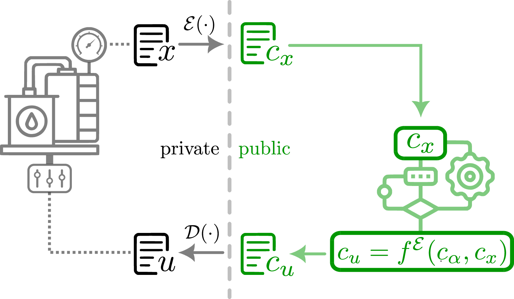
In this paper, we consider the implementation of the later-mentioned FHE scheme to handle the evaluation of the polynomial control law in a fully homomorphic way. By allowing both multiplication and addition operations with encrypted values, we can fully outsource the evaluation of the control law to cloud services. Such an implementation of an FHE-based controller in the closed-loop is depicted in Figure 1.
2.2 Fully Homomorphic Encryption Framework↩︎
In this paper we consider the Brakerski/Fan-Vercauteren (BFV) cryptosystem [7], a member of the FHE frameworks family. The BFV scheme is similar to the Brakerski-Gentry-Vaikuntanathan (BGV) scheme [25], but employs different noise management techniques [26]. Both BGV and BFV are based on the hardness of the Ring Learning With Errors (RLWE) problem [27], which provides strong security guarantees against quantum and classical attacks. In BFV, plaintexts and ciphertexts are represented as polynomials over two distinct rings \[\begin{align} R_{\tau} &= \mathbb{Z}_{\tau} [X]/(X^{\mathcal{N}} + 1) , \tag{3} \\ R_\mathcal{q} &= \mathbb{Z}_{\mathcal{q}} [X]/(X^{\mathcal{N}} + 1) , \tag{4} \end{align}\] where, respectively, 3 is a space for plaintext polynomials with coefficients smaller than plaintext modulus \(\tau\), and 4 represents polynomial space for each coordinate (polynomial) of the ciphertext with coefficients smaller than coefficient modulus \(\mathcal{q}\). Both coefficient moduli ensure that the plaintext and ciphertext operations are performed in the finite fields \(\mathbb{Z}_{\tau}\) and \(\mathbb{Z}_{\mathcal{q}}\), respectively. The size of rings 3 and 4 is defined by polynomial modulus \((X^{\mathcal{N}} + 1)\), a cyclotomic polynomial characterized by a polynomial modulus degree \(\mathcal{N}\).
Since the BFV is built on the RLWE problem, the ciphertext is represented by a tuple of two polynomials, i.e., \(c=(c_{(1)},c_{(2)})\). Thus the polynomial space for ciphertext is defined as \(R_\mathcal{q}^2\), where \(2\) stands for the tuple of two elements. BFV provides an evaluation of both homomorphic additions and multiplications with exact results. The cryptographic scheme within the homomorphic properties of BFV is described in detail in [7].
Since BFV is based on integer numbers, we consider a simple quantization as follows \[\label{eq:quant} m_{\text{I}} = \left\lfloor m \cdot 10^{\theta} \right\rceil ,\tag{5}\] where \(m_{\text{I}}\) is integer form of real-valued message \(m\) regarding the precision degree \(\theta\). In our proposal, we consider encrypted closed-loop as depicted in Fig. 1. In this figure, the states \(x\) and control inputs \(u\) are the real-valued messages \(m\) encrypted to ciphertexts of states \(c_{\text{x}}\) and inputs \(c_{\text{u}}\). The ciphertext of designed polynomial controller is noted as \(c_{\alpha}\), while the evaluation of the control law over ciphertexts is denoted by function \(f^{\mathcal{E}}(\cdot)\).
2.3 Problem Statement↩︎
The main aim of this paper is to design a secure, robust, stable, and easy to implement MPC policy. The security is imposed by using the fully encrypted evaluation of control law, which however induces quantization of control inputs and system states, see 5 . To address this quantization effect one can design a robust MPC policy. Literature provides various methods such as the min-max-like robust MPC [28] or the tube MPC [2] designs to name a few. In this paper we apply the first mentioned approach.
In what follows, we point out that the inherited quantization error 5 has to be considered in the controller design procedure. Specifically, we show that it can be formulated as an additive disturbance in the prediction model, leading to a robust MPC design.
3 Encrypted Model Predictive Controller via Polynomial Approximation↩︎
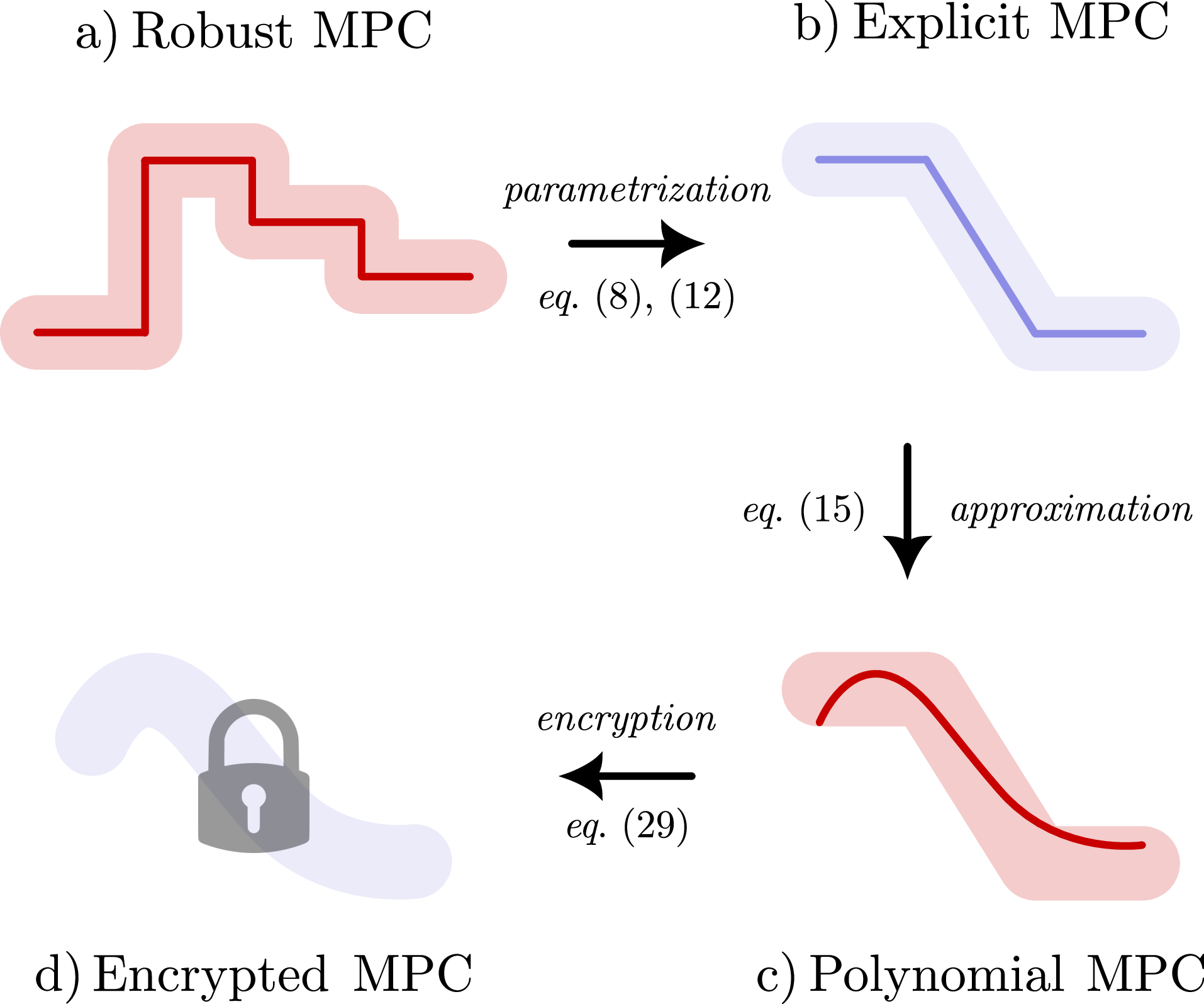
In this section, we show how to approximate the resulting MPC policy by a polynomial feedback law to reduce computational requirements and its memory footprint, hence making the implementation much easier. It should be empathized that all the aforementioned approaches are performed such that the feasibility and stability properties of the original MPC policy are still preserved. The subsequent steps of encrypted approximated MPC design are depicted at Figure 2.
3.1 Robust Encrypted MPC Design↩︎
First, for MPC design purposes, we need a reliable mathematical model predicting the future behavior of the system dynamics. Consider a widely-used linear time-invariant (LTI) system in discrete time domain affected by the interval uncertainties \(f(x(t),u(t),q_\text{x}(t),q_\text{u}(t),d(t))\) defined as \[\label{eq:mpc:theory:sys2} f(\cdot) = A (x(t) + q_\text{x}(t)) + B (u(t)+q_\text{u}(t)) + D d(t),\tag{6}\] with states \(x(t) \in \mathbb{R}^{n_\text{x}}\), inputs \(u(t) \in \mathbb{R}^{n_\text{u}}\), state quantization error \(q_\text{x} \in \mathbb{Q}_{\text{x}} \subset \mathbb{R}^{n_\text{x}}\), input quantization error \(q_\text{u}(t) \in \mathbb{Q}_{\text{u}} \subset \mathbb{R}^{n_\text{u}}\), and process disturbance \(d(t) \in \mathfrak{D} \subset \mathbb{R}^{n_\text{d}}\). We note that both quantization errors \(q_\text{x}(t)\) and \(q_\text{u}(t)\) are within compact polyhedral sets \(\mathbb{Q}_{\text{x}}\) and \(\mathbb{Q}_{\text{u}}\), respectively. Note, the origin of these errors arises from the encoding in 5 , where quantization of real numbers into integers is required. Hence, the prediction model in 6 represents an LTI system under additive uncertainty.
Let us rewrite 6 into its equivalent compact form \[\label{eq:mpc:theory:sys} \widetilde{f}(x(t),u(t),w(t)) = A x(t) + B u(t) + W w(t),\tag{7}\] where \(w(t) = \begin{bmatrix}d^\top(t) & q_\text{x}^\top(t) & q_\text{u}^\top(t) \end{bmatrix}^\top \in \mathbb{R}^{n_\text{d}+n_\text{x}+n_\text{u}}\) and \(W = \begin{bmatrix} D & A & B \end{bmatrix}\). Assume that the system 7 is subjected to non-empty polyhedral sets \[\label{eq:mpc:theory:cons} x(t) \in \mathcal{X}, \;u(t) \in \mathcal{U}, \;w(t) \in \mathcal{W},\tag{8}\] where \(\mathcal{X} \subseteq \mathbb{R}^{n_\text{x}}\), \(\mathcal{U} \subseteq \mathbb{R}^{n_\text{u}}\), and \(w(t) \in \mathcal{W} \subset \mathbb{R}^{n_\text{d}+n_\text{x}+n_\text{u}}\).
We define an MPC problem to drive the system 7 to the origin while fulfilling constraints in 8 as \[\tag{9} \begin{align} J^\star = \min_{\substack{U_{\text{N}}}} \;& \Vert x_{N} \Vert_{Q_{\mathrm{N}}}^n+ \sum_{k=0}^{N-1} \left( \Vert x_{k} \Vert_{Q_{\mathrm{x}}}^n+ \Vert u_{k} \Vert_{Q_{\mathrm{u}}}^n\right) \tag{10}\\ \text{s.t.} \; &x_{k+1} = \widetilde{f}(x_k,u_k,w), \tag{11}\\ &x_k \in \mathcal{X}, u_k \in \mathcal{U}, w_k \in \mathcal{W}, \tag{12}\\ &x_N \in \mathcal{X}_{\mathrm{N}}, \tag{13}\\ &x_0(t) = x(t), \tag{14} \end{align}\] where 11 –12 are enforced for the entire prediction horizon \(N\), i.e., \(k = 0, \dots, N-1\). Next, \(x_k\), \(u_k\), and \(w_k\) denote, respectively, the state, input, and disturbance predicted vectors at prediction step \(k\) and at discrete time \(t\), \(\mathcal{X}_{\mathrm{N}} \subseteq \mathcal{X}\) is the polyhedral robust control invariant terminal set with origin in its interior \(\mathbb{0} \in \mathcal{X}_{\mathrm{N}}\).
n the objective function 10 , \(\Vert x_{N} \Vert_{Q_{\mathrm{N}}}^n\) is the weighted terminal penalty, \(\Vert x_{k} \Vert_{Q_{\mathrm{x}}}^n\) is the weighted state vectors, and \(\Vert u_{k} \Vert_{Q_{\mathrm{u}}}^n\) is the weighted input vectors where \(Q_{\mathrm{x}} \succeq 0\), \(Q_{\mathrm{N}} \succeq 0\), \(Q_{\mathrm{u}} \succ 0\), and norm \(n\in \{1,\infty \}\) is assumed.1 The terminal penalty \(Q_{\mathrm{N}}\) is determined as a solution of Riccati equation of the conventional LQR design problem. The resulting optimization problem 9 can be formulated as a linear program (LP) the solution of which yields a sequence of optimal robust control actions \(U_\text{N} = [u_0^\top, \dots, u_{N-1}^\top]^\top\).
Assumption 1. Assume that
By solving 9 parametrically, i.e., for all feasible \(x(t) \in \mathcal{X}\), we obtain the feedback law \(\mu: \Omega \mapsto \mathcal{U}\) and the corresponding value function \(J^\star: \Omega \mapsto \mathbb{R}_{\geq 0}\) as continuous PWA functions defined over \(\Omega = \cup_{i=1}^M \mathcal{R}_i = \{ x(t) \; | \; \exists u : \eqref{eq:mpc:theory:MPC95cons}-\eqref{eq:mpc:theory:MPC95terminalcon} \;\text{holds}\}\), where \(\mathbb{R}_{\geq 0}\) represents non-negative real numbers, see [28]. Specifically, we define the explicit feedback policy as \[\label{eq:mpc:theory:eMPC:mu} \mu(x(t)) := F_i x(t) + g_i \;\quad \text{if} \;\quad x(t) \in \mathcal{R}_i,\tag{15}\] and the value function as \[\label{eq:mpc:theory:eMPC:obj} J^\star(x(t)) := H_i x(t) + h_i \;\quad \text{if} \;\quad x(t) \in \mathcal{R}_i,\tag{16}\] where \(i = 1, \dots, M\). We say that the polyhedral partition \(\Omega\) consists of \(M\) regions \(\mathcal{R}_i\) with \(\mathop{\mathrm{int}}(\mathcal{R}_i) \cap \mathop{\mathrm{int}}(\mathcal{R}_j) = \varnothing\), \(\forall i \ne j\) holds.2 For the ease of notation, we onward omit the time domain \((t)\), i.e., \(x = x(t)\).
Remark 1 (Quadratic penalty). Note, that 9 with \(n\in \{1,\infty \}\) leads to an LP, which results in 16 . This specific form of the PWA value function is essential for our further results, see selection of a Lyapunov function in Section 3.2. We would like to point out that one can still formulate 9 as a quadratic problem (QP) with \(n=2\), or reformulate 9 as an associated QP of the tube MPC [29]. Then, however, we need to perform an additional procedure to transform the resulting PWQ value function 10 into its corresponding PWA approximation, while preserving its stability properties, see [28] for instance.
Remark 2 (Stability). We recall that by following [30], one can preserve the closed-loop system stability of 9 also without the terminal set constraint 13 , e.g., by the proper tuning of the terminal penalty \(Q_{\mathrm{N}}\) in the cost function 10 and/or by tuning the length of the prediction horizon \(N\) to ensure inactive terminal set constraint 13 , etc.
Definition 1. (Encoded LTI system and control law)
Finally, let the uncertain LTI system 6 be evaluated above the quantization 5 of control inputs \(\hat{u} \in \mathcal{U} \oplus \mathbb{Q}_{\mathrm{u}}\) and
system states \(\hat{x} \in \mathcal{X} \oplus \mathbb{Q}_{\mathrm{x}}\) such that uncertain LTI system 6 is equivalent to the following system in the compact form \[\label{eq:mpc:theory:sys:encrypted} \hat{f}(\hat{x}(t),\hat{u}(t),d(t)) = A \hat{x}(t) + B \hat{u}(t) + D d(t),\qquad{(1)}\] where \(\hat{x}(t) = x(t)
+ q_\text{x}(t)\) and \(\hat{u}(t) = u(t)+q_\text{u}(t)\). Then, the corresponding control law of explicit MPC in 15 is evaluated in its quantized form given by \[\label{eq:mpc:theory:eMPC:mu:quantize} \hat{\mu}(\hat{x}(t)) := F_i \hat{x}(t) + g_i \;\quad \text{if} \;\quad \hat{x}(t) \in \mathcal{R}_i,\qquad{(2)}\] for \(\forall i = 1, \dots, M\).
Lemma 1. Consider explicit control law 15 of robust MPC design problem in 9 exists, and Assumption 1 holds. Then the corresponding control law in ?? ensures closed-loop system stability and recursive feasibility subject to the uncertain LTI system in 7 for all states \(x(t) \in \Omega\) w.r.t. any realization of the quantization error \(q_\text{x}(t)\), \(q_\text{u}(t)\), and the process disturbance \(d(t)\) from \(\begin{bmatrix}d^\top(t) & q_\text{x}^\top(t) & q_\text{u}^\top(t) \end{bmatrix}^\top \in \mathcal{W}\).
Proof. Proof consists of two main parts. First, we prove that the system in 7 is closed-loop stable and recursive feasibility under the control law 15 . Let Assumption 1 hold. It directly follows from [28], that if there exists a feasible solution of robust MPC design problem in 9 , then control law 15 satisfies the closed-system stability of 7 and recursive feasibility of optimization problem 9 for any feasible \(x_{0}\).
Secondly, it remains to prove that these properties are preserved also w.r.t. quantize control law in ?? constructed above the feasible set of quantize system states \(\hat{x}\). As the original uncertain LTI system 6 is equivalent to its expanded form given by \[\begin{align} \label{prf:quantize95system} f(\cdot) = A x(t) + B u(t) + \underbrace{ A q_{\mathrm{x}}(t) + B q_{\mathrm{u}}(t) + D d(t) }_{W w(t)} , \end{align}\tag{17}\] for \(w(t) = \begin{bmatrix}d^\top(t) & q_\text{x}^\top(t) & q_\text{u}^\top(t) \end{bmatrix}^\top \in \mathbb{R}^{n_\text{d}+n_\text{x}+n_\text{u}}\) and \(W = \begin{bmatrix} D & A & B \end{bmatrix}\), it is directly resulting in the equivalence of 17 to the uncertain LTI system in 7 . In terms of the equivalent prediction model 11 , it follows that any feasible solution of 9 simultaneously satisfies the recursive feasibility w.r.t. quantize control inputs and system states in 17 , since 17 \(\Leftrightarrow\) 6 holds. This leads to 17 being equivalent to ?? . Consequently, according to Definition 1, for any \(\Vert q_{\mathrm{x}} \Vert_{\infty} \in \mathbb{Q}_{x}\), the associated quantize system state \(\hat{x}(t) = x(t) + q_{\mathrm{x}}(t)\) leads to the quantized control law in ?? , such that the corresponding worst-case quantize error by design satisfies
\[\label{prf:quantize95control95input} \begin{align} \Vert \hat{\mu}(\hat{x}(t)) - \mu(x(t)) \Vert_{\infty} = \Vert \hat{u}(t) - u(t) \Vert_{\infty} &= \Vert q_{\mathrm{u}} \Vert_{\infty}, \\ \Vert q_{\mathrm{u}} \Vert_{\infty} &\in \mathbb{Q}_{u}. \end{align}\tag{18}\] Finally, in terms of 17 constructed subject to any impact of the uncertainty \(W w(t)\), including the bounded quantize errors for \(\forall q_{\mathrm{u}} \in \mathbb{Q}_{\mathrm{u}}\), \(\forall q_{\mathrm{x}} \in \mathbb{Q}_{\mathrm{x}}\), and under the equivalence of 17 \(\Leftrightarrow\) 7 , it directly follows that for any feasible solution \(x(t) \in \Omega\) of 9 , the corresponding \(\hat{\mu}(\hat{x}(t))\) in ?? leads to the recursive feasible and stabilizing control action \(\hat{u}(t)\). \(\Box\) ◻
Remark 3 (Non-robust case). The benefit of the proposed robust MPC design framework is stability guarantees, and, simultaneously, the increased application range subject to the plant-model mismatch and/or other external disturbances. If one needs to reduce the conservativeness by omitting the robust nature of the MPC formulation, then consider \(\mathfrak{D}\) in 6 , ?? to be an empty set.
3.2 Parametric Solution with Polynomials↩︎
In this paper we adopt results from [31] based on which we approximate 15 by a new polynomial control law \[\label{eq:mpc:app:tmu} \widetilde{\mu}(x) = \alpha_1 x + \alpha_2 x^2 + \dots + \alpha_{\kappa} x^{\kappa},\tag{19}\] that stabilizes the system 7 and provides recursive satisfaction of the constraints 8 . The coefficients to be find are \(\boldsymbol{\alpha} = \{\alpha_i, \dots, \alpha_{\kappa}\}\), \(\kappa\) is the fixed polynomial degree, and \(x^i = [x_1^i, x_2^i, \dots, x_{n_{\mathrm{x}}}^i]^\top\) is the element-wise power of the state vector \(x \in \mathbb{R}^{n_{\mathrm{x}}}\).
Let us assume that for the closed-loop system \(f_{\text{CL}}(x,w) := \widetilde{f}(x,\mu(x),w)\) there exists a PWA Lyapunov function \(L : \Omega \mapsto \mathbb{R}_{\geq 0}\) that satisfies \(L(f_{\text{CL}}(x,w)) \leq \gamma L(x)\) and \(L(\mathbb{0}^{n_\text{x}}) = 0\) for some \(\gamma \in [0,1)\), \(\forall x \in \Omega\), and \(\forall w \in \mathcal{W}\). 3
For the system 7 , Lyapunov function \(L(\cdot)\), and a fixed \(\gamma\) we construct stabilizing tube [34]: \[\label{eq:mpc:app:tube} \begin{align} \mathcal{T}(L,\gamma) \! := \! \begin{Bmatrix} \left[x^\top, u^\top \right]^\top \, \!\! \vert & \!\!\!\!\!\!\!\!\!\! \, u \in \mathcal{U}, x \in \Omega, \widetilde{f}(x,u,w) \in \Omega, \\ & \!\!\!\!\!\! L(\widetilde{f}(x,u,w)) \leq \gamma L(x), \forall w \in \mathcal{W} \end{Bmatrix} \! . \end{align}\tag{20}\]
As \(\text{dom}(L) = \Omega = \cup_{i=1}^M \mathcal{R}_i\), we have that \(\mathcal{T}(L,\gamma) := \cup_{i=1}^{M} \mathcal{T}_i\) with \(\mathcal{T}_i := \cup_{j=1}^{M} \mathcal{T}_{i,j}\) for all \(i = 1, \dots, M\). Respectively, the entire stability tube is defined as union of polytopes \(\mathcal{T}(L,\gamma) := \cup_{i=1}^{M} \cup_{j=1}^{M} \mathcal{T}_{i,j}\) where each \(\mathcal{T}_{i,j} \in \mathbb{R}^{n_x+n_u}\) represents a feasible transition from \(\mathcal{R}_i\) to \(\mathcal{R}_j\) for which the value of \(L(\cdot)\) decreases.
Let us define each region \(\mathcal{R}_i\) of \(\Omega\) in its vertex representation \[\begin{align} \label{eq:mpc:app:region95vertex} \mathcal{R}_i &= \begin{Bmatrix} x \, | \, x = \sum_{j=1}^{|\nu_i|} \lambda_j |\nu_i|_j, \lambda \in \Lambda_i \end{Bmatrix},\\ \Lambda_i &= \begin{Bmatrix} \lambda \, | \, 0 \leq \lambda_j \leq 1, \sum_{j=1}^{|\nu_i|}\lambda_j=1 \end{Bmatrix}, \end{align}\tag{21}\] where \(\nu_i\) are vertices of \(\mathcal{R}_i\), \(|\nu_i|_j\) is the \(j\)-th vertex of \(\mathcal{R}_i\), and \(|\cdot|\) denotes cardinality. Assume that for a given \(V(\cdot)\) and a fixed \(\gamma \in [0,1)\) there exists a full-dimensional stability tube \(\mathcal{T}(L,\gamma)\) that is composed of \(i = 1,\dots, M\) polytopes4 \[\label{eq:mpc:app:subtube} \mathcal{T}_i := \begin{Bmatrix}\left[x^\top, u^\top\right]^\top \, | \, \left[T^{\mathrm{x}}_{i} T^{\mathrm{u}}_{i}\right] \left[x^\top, u^\top\right]^\top \leq T^0_i \end{Bmatrix},\tag{22}\] with the connected union \(\cup_{i=1}^{M} \mathcal{T}_i\). By plugging 19 into 22 and substituting the state vector \(x\) by vertices of \(\mathcal{R}_i\) per 21 we obtain a set of polynomials \[\label{eq:mpc:app:poly} \rho_i(\boldsymbol{\alpha},\lambda) := T^0_i - T^x_i \lambda - T^u_i \widetilde{\mu}(\lambda), \, \quad \lambda \in \Lambda_i,\tag{23}\] for all \(i = 1, \dots, M\). These polynomials can be further homogenized by multiplying single monomials with \(\left(\sum_{j=1}^{|\nu_i|}\lambda_j\right)\) until all have the same degree. The Pólya’s polynomials can be then defined as follows \[\label{eq:mpc:app:homogen} \rho_i^\varphi(\boldsymbol{\alpha},\lambda) = \rho_i(\boldsymbol{\alpha},\lambda) \cdot \left(\sum_{j=1}^{|\nu_i|}\lambda_j\right)^\varphi,\tag{24}\] where \(\varphi\) is a Pólya degree, see [35].
Finally, as shown in [31], if a stabilizing Lyapunov function \(L(\cdot)\) and a stability tube \(\mathcal{T}(L,\gamma)\) satisfying all the aforementioned assumptions can be constructed, then the coefficients \(c_i^\varphi\) of the Pólya polynomials 24 can be defined symbolically. Subsequently, the following linear program \[\tag{25} \begin{align} \min_{\boldsymbol{\alpha}} \;& z(\cdot) \tag{26}\\ \text{s.t.} \; &c_i^\varphi \geq 0 \, , \, i = 1,\dots, M \tag{27} \end{align}\] can be solved to obtain coefficients \(\boldsymbol{\alpha}\) of the approximated control law \(\widetilde{\mu}(x)\) as in 19 that stabilizes the system 7 , while providing recursive feasibility of the original constraints in 8 . Note, there are multiple alternatives how to define the objective function 26 . The most straightforward one is to choose \(z(\cdot) = 0\), i.e., state 25 as a pure feasibility problem. Another option is to minimize the point-wise distance between the original and the approximated control policy over selected points from \(\Omega\). One suitable candidate is to choose vertices of each region \(\mathcal{R}_i\), i.e., \(z(\cdot) = \sum_{i=1}^M \sum_{j=1}^{|\nu_i|} ||\mu(\nu_{i,j}) - \widetilde{\mu}(\nu_{i,j})||^n\) with \(n\in {\{1,\inf\}}\).
Corollary 1. Consider the approximated control law 19 of robust MPC design problem in 9 is given to satisfy 25 , and let Assumption 1 hold. If approximated control law \(\widetilde{\mu}(x)\) in 19 ensures the closed-loop system stability and recursive feasibility of 9 for any \(x(t) \in \Omega\), then also \(\widetilde{\mu}(\hat{x})\) according to Definition 1 preserves these properties w.r.t. any realization of the bounded quantization error \(q_\text{x}(t)\), \(q_\text{u}(t)\), and the process disturbance \(d(t)\) from \(\begin{bmatrix}d^\top(t) & q_\text{x}^\top(t) & q_\text{u}^\top(t) \end{bmatrix}^\top \in \mathcal{W}\).
Proof. The proof has two parts. First, we need to prove that the approximated control law \(\widetilde{\mu}(x)\) in 19 satisfies the closed-loop system stability and the recursive feasibility of 9 for any feasible \(x \in \Omega\). We recall Lemma 3.5. in [31] implying that for any feasible solution \(\boldsymbol{\alpha}\) of 25 the resulting control law \(\widetilde{\mu}(x)\) in 19 preserves by design the closed-loop stability of system 6 and the recursive feasibility subject to the constrained system states and control inputs in 9 .
Secondly, it remains to prove that also the approximated control law \(\widetilde{\mu}(\hat{x})\) in 19 evaluated for quantize system state \(\hat{x}(t) = x(t) + q_{\mathrm{x}}(t)\) preserves the closed-loop system stability and recursive feasibility for any \(q_{\mathrm{x}} \in \mathbb{Q}_{x}\), \(q_{\mathrm{u}} \in \mathbb{Q}_{u}\), and \(d \in \mathfrak{D}\) in system 7 . By substituting any bounded quantization errors \(q_{\mathrm{u}} \in \mathbb{Q}_{u}\), \(q_{\mathrm{x}} \in \mathbb{Q}_{x}\) into 17 , it follows from Lemma 1 and the from equivalence of 17 and 7 , that \(\widetilde{\mu}\) by design ensures closed-loop system stability and recursive feasibility of \(\widetilde{\mu}(\hat{x})\) in 19 for any feasible \(\hat{x} \in \Omega\). \(\Box\) ◻
4 Experimental Validation of Encrypted MPC↩︎
This section presents a step-by-step implementation of secured control with encrypted control law in the form of 19 in a closed-loop control scenario. We explore the parameter settings of the BFV implementation
and test it on a laboratory device, where the applicability of the polynomial approximation is clearly visible as well as the effects of the BFV settings on the closed-loop system. The Python language was used to simulate and evaluate results
from encrypted closed-loop process control. All experiments were performed on a \(64\)-bit operating system \(16\)-core CPU with \(\SI{3.4}{\giga\hertz}\)
processor and \(\SI{128}{\giga\byte}\) of RAM. All computations were performed in a single-threaded mode.
4.1 Laboratory Device Flexy \(2.0\)↩︎
We demonstrate the presented control algorithm on single-input single-output laboratory device Flexy \(2.0\) designed as a benchmark laboratory system for control applications, with detailed parameters given in [36]. Manipulated variables are represented by fan speed defined in percentage. The fan produces an airflow bending the flex resistor, thus changing the electric resistance which is the output variable measured in percentage. The appearance of Flexy \(2.0\) is depicted in Figure 3.

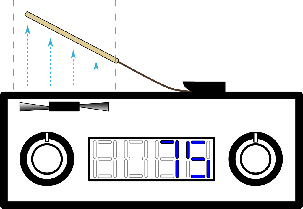
Figure 3: Laboratory device Flexy \(2.0\) with a flex-bend as controlled variables and fan-speed as manipulated variable..
We adopt the linear model of Flexy \(2.0\) from [37] in the form of a continuous transfer function defined as \[G(s) = \frac{0.89}{0.66s + 1}\] which is further transformed into a discrete time state space model
\[x(t+T_\text{s}) = 0.966 \, x(t) + 0.101 \, u(t), \label{eq:process}\tag{28}\] with sampling period \(T_\text{s} = \SI{10}{\milli\second}\). By considering both quantization and process disturbance errors, i.e., \(w(t) = \begin{bmatrix}d^\top(t) & q_\text{x}^\top(t) & q_\text{u}^\top(t) \end{bmatrix}^\top\), the final uncertain linear time-invariant model 7 is represented by \[\begin{array}{rl} x(t+T_\text{s}) = &0.966 \, x(t) + 0.101 \, u(t) + \\ &\underbrace{\begin{bmatrix} 1.000 & 0.966 & 0.101 \end{bmatrix}}_W\, \;w(t), \label{ikvhlxcs} \end{array}\tag{29}\] and is utilized for the MPC design in 11 .
Flexy device represents a laboratory-scale benchmark for systems that mimic the challenges of controlling industrial devices such as:
satisfying physical constraints,
handling the systems with fast dynamics,
signal filtering and processing,
limitation of the device’s microcontroller to handle measurements and apply control actions,
while respecting the sampling period at the level of milliseconds.
4.2 Encrypted Control Setup↩︎
This section describes the control setup suitable for the use of the BFV scheme in secured process control. The encrypted MPC approach is implemented according to the scheme in Figure 4.

We consider TenSEAL library [38] which is a Python implementation of Microsoft SEAL [39]. For use of the BFV scheme, the following parameters have to be set:
Polynomial modulus degree (\(\mathcal{N}\)) defining the maximal degree of each polynomial in polynomial space \(R\). Parameter \(\mathcal{N}\) has to be positive and a power of \(2\), typically \(\mathcal{N} \in \{ 2\,048, 4\,096, \dots \}\). The security level increases with growing \(\mathcal{N}\). However, higher \(\mathcal{N}\) means higher computational complexity, thus the evaluation of mathematical operations over ciphertexts is slower. In
TenSEALis degree \(\mathcal{N}\) a mandatory parameter, thus it has to be defined.Plaintext modulus (\(\tau\)) used to handle the coefficient size of plaintexts. This parameter has to be a prime and basically represents the largest number that can be encoded and encrypted. The value of \(\tau\) is selected such that \(\mod(2\mathcal{N},\tau)=1\). Plaintext modulus \(\tau\) is a mandatory parameter.
Two parameters \(\mathcal{N}\) and \(\tau\) are elements of a structure called context, and are user-defined settings. Finally, to perform homomorphic multiplications we generate relinearization(evaluation) keys to handle the size of resulting ciphertexts.
Since the majority of control applications operate with floating point values, we adjust states and controller coefficients into integers with relation 5 , hence \[\begin{align} x_{\text{I}} &= \left\lfloor x \cdot 10^{\theta_{\text{x}}}\right\rceil, \tag{30}\\ \boldsymbol{\alpha}_{\text{I}} &= \left\lfloor\boldsymbol{\alpha} \cdot 10^{\theta_{\alpha}}\right\rceil, \tag{31} \end{align}\] where in \(x_{\text{I}}\) is integer value of state \(x\) with precision degree \(\theta_{\text{x}}\) and \(\boldsymbol{\alpha}_{\text{I}}\) is polynomial controller with integer coefficients with precision \(\theta_{\alpha}\).
Next, we present the implementation of encrypted polynomial closed-loop control for single-input single-output systems:
Modify states: first, we adjust the measured state \(x\) to vector form \(\mathbf{x}\) with respect to the order of the polynomial controller, hence \[\mathbf{x} = \begin{bmatrix} x, & x^2, & \dots, & x^\kappa \end{bmatrix}, \label{eq:states:extend}\tag{32}\] where \(\kappa\) is the order of the polynomial controller.
Adjust to integers: next, we convert \(\mathbf{x}\) to integer vector \(\mathbf{x}_{\text{I}}\) with precision degree \(\theta_{\text{x}}\) by using 30 element-wise, hence \[\mathbf{x}_{\text{I}} = \left\lfloor\mathbf{x} \cdot 10^{\theta_{\text{x}}}\right\rceil. \label{eq:states:ajust}\tag{33}\] We encode and encrypt \(\mathbf{x}_{\text{I}}\) send ciphertext \(c_{\mathbf{x}_{\text{I}}} = \mathcal{E}(E(\mathbf{x}_{\text{I}}))\) to the control unit.
Evaluate control law: the encrypted controller is represented by ciphertext \(c_{\boldsymbol{{\alpha}}_{\text{I}}} = \mathcal{E}(E(\boldsymbol{{\alpha}}_{\text{I}}))\) obtained by encrypting polynomial controller in integer form \(\boldsymbol{{\alpha}}_{\text{I}}\) 31 with precision degree \(\theta_{\alpha}\). We evaluate the control law 19 over ciphertexts \(c_{\mathbf{x}_{\text{I}}}\) and \(c_{\boldsymbol{{\alpha}}_{\text{I}}}\) and return ciphertext of the encrypted control input \(c_{u_{\text{I}}}\) computed as \[c_{u_{\text{I}}} = f^{\mathcal{E}}(c_{\boldsymbol{{\alpha}}_{\text{I}}}, c_{\mathbf{x}_{\text{I}}}) = \sum_{i=1}^{\kappa} c_{\boldsymbol{{\alpha}}_{\text{I}}, (i)} \cdot c_{\mathbf{x}_{\text{I}}, (i)} \label{eq:sec:ctrl}\tag{34}\] which basically represents the scalar product of two encrypted vectors represented by ciphertexts \(c_{\boldsymbol{{\alpha}}_{\text{I}}}\) and \(c_{\mathbf{x}_{\text{I}}}\).
Rescale control input: encrypted control input is decrypted and rescaled back by relation \[u = \frac{D(\mathcal{D}(c_{u_{\text{I}}}))}{10^{(\theta_{\text{x}}+\theta_{\alpha})}},\] where \(u\) is the control input ready to be applied to the process. The control algorithm 5 includes all of the necessary steps for encrypted polynomial control considering BFV framework.

Note that both polynomial controllers and states are represented by a single ciphertext and controller \(\boldsymbol{\alpha}\) is adjusted to integers and encrypted only once. The control law evaluated over ciphertexts (Algorithm \(1\), line \(7\)) respects the relation 19 .
The presented control setup will ensure the encrypted polynomial control with the use of the BFV cryptographic scheme.
4.3 Results and Discussion↩︎
We construct an MPC controller for system 28 , where states are subjected to \(|x| \leq 4\) and control inputs to \(|u| \leq 1\). By solving 9 with \(n= 1\), \(N = 10\), \(Q_{\mathrm{u}} = 1\), \(Q_{\mathrm{x}} = 10\), and \(\mathcal{W}\) was such that \(-0.05 \leq {\begin{bmatrix} 1.000 & 0.966 & 0.101 \end{bmatrix}} w(t) \leq 0.05\), we obtained the explicit feedback law as in 15 defined over \(M = 14\) regions constructed in \(0.4856\) seconds. The memory footprint of this controller was \(0.84\) kB. By choosing \(J^\star(\cdot) = L(\cdot)\) and selecting \(\gamma = 0.99\) we synthesized the stabilizing tube 20 .
The LP problem in 25 was constructed in YALMIP [40] with \(\kappa=
3\), \(\varphi = 1\), and \(z(\cdot) = \sum_{i=1}^M \sum_{j=1}^{|\omega_i|} ||\mu(\omega_{i,j}) - \widetilde{\mu}(\omega_{i,j})||^1\), where \(\omega_{i}\) is a grid of \(10\) equidistantly split points across the region \(\mathcal{R}_i\), i.e., \(|\omega_i| = 10\). The
solution of 25 , formulated in YALMIP within \(7.29\) seconds and solved via GUROBI in \(1.11\) seconds, was the stabilizing
polynomial feedback law as in 19 with \[\boldsymbol{\alpha} = \begin{bmatrix} 0.0000, -2.3110, 0.0098, 0.00078 \end{bmatrix},
\label{eq:controller}\tag{35}\] with the memory footprint of \(0.2\) kB. To determine the suboptimality of \(\widetilde{\mu}(\cdot)\) w.r.t. \(\mu(\cdot)\), we have split the domain \(\Omega\) into \(100\) equidistantly divided points and used them as initial conditions for closed-loop profiles. The
suboptimality was computed as \((J^\star - \widetilde{J})/J^\star \, 100\,\% = 56\,\%\) where \(J^\star\) and \(\widetilde{J}\) are the overall values of 10 for the feedback law \(\mu(\cdot)\) and \(\widetilde{\mu}(\cdot)\), respectively, within all performed simulations. The graphical comparison of these
controllers is presented in Figure [fig:approxeMPC].

We consider a control law 19 with polynomial controller 35 in the task of disturbance rejection, while respecting the steady state values \(x_{\text{s}} = \SI{73}{\percent}\) and \(u_{\text{s}} = \SI{50}{\percent}\). The experiment of encrypted polynomial control included two various configurations of the BFV framework. We fix the polynomial modulus degree \(\mathcal{N} = 4\,096\) and generate two different values of plaintext modulus \(\tau\) for given \(\mathcal{N}\) and precision degrees \(\theta_{\text{x}}\) and \(\theta_{\alpha}\) with Algorithm 7

where the initial value of \(\tau\) consists of precision for state measurement \(\theta_{\text{x}}\), precision for polynomial controller \(\theta_{\alpha}\) and some additional space for computations represented by adding \(1\). Function \(\texttt{nextPrime}(v)\) generates prime larger than \(v\). For each experiment, we measure the maximal \(t_{\text{max}}\) and average \(t_{\text{avg}}\) computational time of evaluating control law 34 over ciphertexts. The analysis was realized for time span of \(t_{\text{exp}} = \SI{30}{\second}\) during which we introduced a control input disturbances \(d_1 = \SI{0}{\percent}\) and \(d_2 = \SI{100}{\percent}\) at times \(t_{\text{d}_1} = \SI{10}{\second}\) and \(t_{\text{d}_2} = \SI{20}{\second}\), respectively. Both disturbances lasted \(\SI{0.5}{\second}\). The experimental setups \(\mathcal{S}_1\) and \(\mathcal{S}_2\) along with their computational performance results are listed in Table 1. The graphical results of both experiments are presented in Figure 8.
| \([\SI{}{\milli\second}]\) | ||||||
| \([\SI{}{\milli\second}]\) | ||||||
| \(S_1\) | \(4\,096\) | \(1\,032\,193\) | \(1\) | \(4\) | \(\SI{3.4}{}\) | \(\SI{6.3}{}\) |
| \(S_2\) | \(4\,096\) | \(100\,016\,129\) | \(3\) | \(4\) | \(\SI{3.3}{}\) | \(\SI{5.5}{}\) |

Reading out from the results depicted in Figure 8 it is obvious that the presented control algorithm worked well with both setups of the BFV scheme. For \(\tau_1=1\,032\,193\), the maximal computational time was \(t_{\text{max}} = \SI{6.3}{\milli\second}\) and the average time \(t_{\text{avg}} = \SI{3.4}{\milli\second}\). Both times remained within the interval of sampling period \(T_{\text{s}} = \SI{10}{\milli\second}\). For the setup with \(\tau_2=100\,016\,129\) were the computational times at the same level as for the first setup (\(t_{\text{max}} = \SI{5.5}{\milli\second}\), \(t_{\text{avg}} = \SI{3.3}{\milli\second}\)), since \(\mathcal{N}\) is fixed, thus the computational complexity remains unchanged. Finally, we have also computed average quantization errors of states \(q_\text{x}\) and control actions \(q_\text{u}\). For the setup with \(\tau_1=1\,032\,193\) we have detected \(q_\text{x} = 170.0\cdot10^{-4}\) and \(q_\text{u} = 41\cdot10^{-4}\), while for the setup \(\tau_2=100\,016\,129\) we obtained \(q_\text{x} = 1.7\cdot10^{-4}\) and \(q_\text{u} = 0.6\cdot10^{-4}\).
5 Conclusions↩︎
Addressing data and controller privacy with homomorphic encryption strategies and considering explicit model predictive control and its versatile deployment, the proposed novel control method eliminates the complexity of online optimization or the necessity to solve the point location problems in encryption frameworks. By merging the fully homomorphic encryption frameworks with the polynomial approximation of the explicit model predictive controller, we achieved cryptographically secured close-to-optimal constrained process control, which has not been done so far. This manuscript also presents an experimental implementation and validation in a laboratory-scaled setup that confirms the viability of this encrypted polynomial control, guaranteeing stability, recursive feasibility, and data security. This research not only significantly contributes to the academic domain but also provides industries with a path to data safety in cloud-based control applications.
Acknowledgments↩︎
The authors gratefully acknowledge the contribution of the Scientific Grant Agency of the Slovak Republic under the grants 1/0339/26, 1/0239/24, the Slovak Research and Development Agency under the project APVV-24-0007, and the Research and Innovation Authority (VAIA) under the grant no. 09I01-03-V04-00024 (Slovak Research Excellence in Advanced Control for Smart Industries). M. Klaučo is also supported by the European Union project ROBOPROX (Reg. No. CZ.02.01.01/00/22_008/0004590).
References↩︎
For an arbitrary \(z \in \mathbb{R}^{n_\text{z}}\) we denote norm \(n = 1\) as \(\Vert z \Vert_{Q_{\mathrm{N}}}^1 =\sum_{i=1}^{n_\text{z}} |z_i|\) and for \(n = \infty\) as \(\Vert z \Vert_{Q_{\mathrm{N}}}^{\infty} =\max_{i} |z_i|\).↩︎
We denote \(\mathop{\mathrm{int}}(\mathcal{R}_i)\) to be interior of the \(i\)-th region.↩︎
It was shown by many authors [32], [33] that by carefully choosing the optimization problem 9 then \(\mu(x)\) provides closed-loop system stability and the value function \(J^\star (x)\) as in 16 can be used as a Lyapunov function for the \(f_{\text{CL}}\), i.e., \(L := J^\star (x)\).↩︎
It is required that \(\mathcal{T}_i\) is a polytope or there exits an inner polytopic approximation that covers the entire state space of \(\mathcal{R}_i\), i.e., \(\text{proj}_x\mathcal{T}_i = \mathcal{R}_i\).↩︎