A Deep Learning Framework for Predicting Solar EUV Irradiance During Significant Flares
July 21, 2026
Abstract
We present FlareEUV, a multimodal deep learning framework for predicting daily extreme ultraviolet (EUV) irradiance at 6.5 nm over three consecutive days during significant solar flares, using multi-instrument observations from NASA’s Solar Dynamics Observatory (SDO). We consider 33 significant flares in the period between 2011 and 2014 in Solar Cycle 24. The SDO observations include 13 co-aligned full-disk images, comprising eight AIA EUV/UV and five HMI magnetic/continuum products. FlareEUV learns the relationship between magnetic structure and coronal emission from the raw imaging data using a lightweight attention-based architecture. Our experimental results demonstrate the good performance of FlareEUV in short-term EUV irradiance forecasting during the significant flares and its superiority over baseline methods.
Multimodal deep learning, EUV irradiance, Space weather
1 Introduction↩︎
The Sun’s extreme ultraviolet (EUV) irradiance plays a central role in controlling the thermosphere–ionosphere energy balance, satellite drag, and radio-wave propagation. During major solar flares, EUV output can change rapidly, particularly in the 6.5 nm band dominated by high-temperature Fe XVIII and Fe XX emissions [1]. Accurate short-term forecasting of this wavelength is therefore essential for space–weather modeling and operational risk mitigation [2].
Traditional proxies such as F10.7 and Mg II reproduce long-term solar variability, but fail to capture the rapid flare-driven dynamics that dominate short-term EUV evolution [3]. A more data-driven alternative is to identify mappings between solar observations and EUV irradiance and use them to forecast flare-specific irradiance evolution. A major source of such observations is NASA’s Solar Dynamics Observatory (SDO), which provides continuous full-disk imaging from the Atmospheric Imaging Assembly (AIA) and vector magnetic-field measurements from the Helioseismic and Magnetic Imager (HMI) [4]–[6]. These instruments encode rich spatial and magnetic structures—such as sunspot complexity, coronal loop brightness, and polarity inversion lines—which correlate strongly with flare-associated EUV enhancements [1], [7], [8].
In this work, we address the following short-term flare-specific EUV irradiance forecasting problem: given temporally aligned multi-channel AIA and HMI observations surrounding a major solar flare at day \(T_{0}\), the goal is to predict the daily solar EUV irradiance at 6.5 nm for three consecutive days: \(T_{0}\) (flare onset/start day), \(T_{1}\) (= \(T_{0}\) + 1 day), and \(T_{2}\) (= \(T_{0}\) + 2 days). The solar EUV irradiance at 6.5 nm data are extracted from the SDO/EVE Level 3 archive available at the LASP Interactive Solar Irradiance Datacenter (LISIRD) (https://lasp.colorado.edu/lisird/).
The 6.5 nm wavelength is dominated by high-temperature Fe XVIII and Fe XX emission lines formed at coronal temperatures of 6–10 MK [1], making it a sensitive diagnostic of post-flare heating and magnetic energy dissipation in the upper corona. SDO/EVE Level 3 irradiance data provide radiometrically calibrated, daily-averaged full-disk measurements integrated over each UTC day, ensuring temporal consistency and reproducibility across events. These measurements serve as the reference standard for scientific analysis and operational space-weather forecasting, as they directly quantify the total solar EUV energy input to Earth’s thermosphere and ionosphere [2].
We consider significant flares during the period between 2011 and 2014 in Solar Cycle 24. There are 33 flare events in the period, taken from FlareDB [9], whose goal is to help scientists understand the onset of solar eruptions, such as flares and coronal mass ejections. Each flare event in FlareDB is classified as M5.0 or greater (including the X-class) according to NOAA Space Weather Prediction Center (SWPC) event reports. These events span a wide range of active-region morphologies and energy-release profiles, providing a diverse benchmark for flare-specific irradiance forecasting. Each flare event in FlareDB is associated with the flare start time, peak time, end time, as well as full-disk images acquired by SDO including eight AIA EUV/UV channels (94, 131, 171, 193, 211, 304, 335, 1600 Å) and five HMI magnetic/continuum products (Bfield, Bincl, Bazim, IC, M) that are in 24 hours before, and 6 hours after the flare event.
1.1 Data Description↩︎
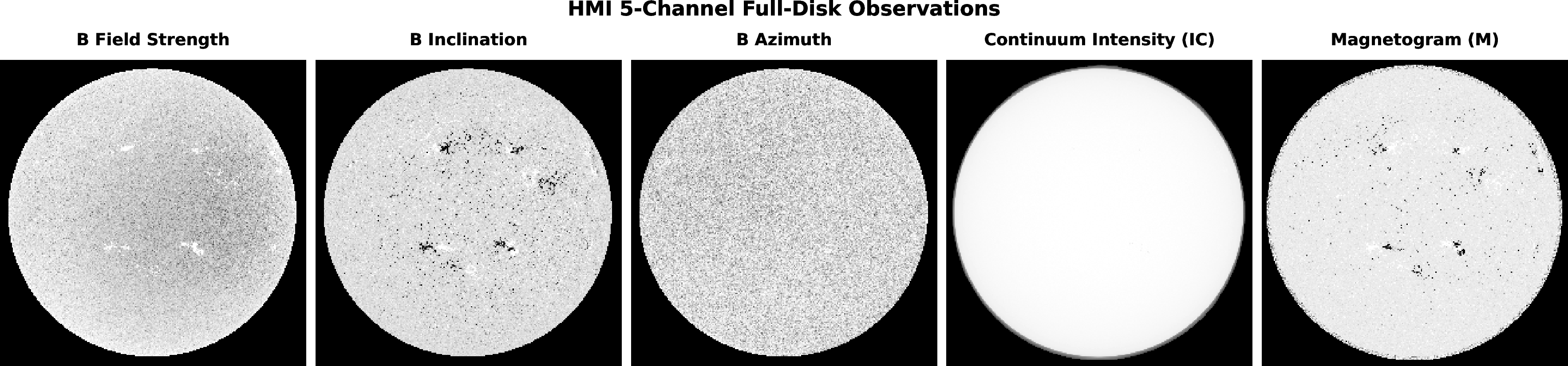
Figure 1 shows the distribution of EVE 6.5 nm irradiance targets on the three forecast days \(T_0\), \(T_{1}\), \(T_{2}\) for all 33 flare events. The box plots show the median (thick line), interquartile range (box), and full data range (whiskers) in each day. Figures 2 and 3 show preprocessed AIA and HMI images for a representative M6.6 flare event in the active region (AR) NOAA 11158. AIA provides multi-wavelength EUV and UV observations tracing plasma across a wide temperature range, while HMI provides vector magnetic-field measurements and continuum structure from the photosphere. Together, these 13 channels form the harmonized input cube used for model training and testing.


1.2 Problem Formulation↩︎
We formulate the problem at hand as a supervised regression task in which pre-flare multi-instrument solar observations are mapped to post-flare irradiance evolution. Specifically, at each time step, we consider a fused set of 13 co-aligned full-disk images acquired by SDO, including eight AIA EUV/UV channels (94, 131, 171, 193, 211, 304, 335, 1600 Å) and five HMI magnetic/continuum products (Bfield, Bincl, Bazim, IC, M). All images were preprocessed to \(256{\times}256\) pixels with a consistent north-up orientation.
Let \(\mathbf{X}_{t} \in \mathbb{R}^{13 \times 256 \times 256}\) denote the fused multi-instrument observation at temporal offset \(t\) relative to the flare start time \(T_{0}\). We sample five pre-flare time steps (see Fig. 4): \[t \in \{-24, -18, -12, -6, 0\}\;\text{hours},\] where \(t = 0\) denotes the flare start time \(T_{0}\). The input to the FlareEUV model consists of the five multi-instrument observations: \[\mathbf{X} = [\mathbf{X}_{-24}, \mathbf{X}_{-18}, \mathbf{X}_{-12}, \mathbf{X}_{-6}, \mathbf{X}_{0}],\] which are temporally averaged (mean-pooled) per channel during preprocessing into a single fused tensor \(\mathbf{X} \in \mathbb{R}^{13 \times 256 \times 256}\). The target output is the vector of daily EUV irradiance values at 6.5 nm: \[\mathbf{Y} = [Y_{T_0},\, Y_{T_1},\, Y_{T_2}] \in \mathbb{R}^{3},\] where \(Y_{T_d}\) corresponds to the EUV irradiance for day \(d \in \{0,1,2\}\) with \(T_1 = T_0 + 24\) h and \(T_2 = T_0 + 48\) h. Thus, the forecasting task at hand is defined as: \[f_{\theta}: \mathbb{R}^{13 \times 256 \times 256} \rightarrow \mathbb{R}^{3},\] where \(f_{\theta}\) is a learnable deep neural network, trained on the major flares considered in the study.

1.3 Contributions of the Work↩︎
Our work makes the following methodological and experimental advances for flare-specific EUV irradiance forecasting:
1. Unified 13-channel multimodal fusion. To solve the problem at hand, we propose FlareEUV, a lightweight multimodal deep learning framework that integrates EUV/UV radiative structure (AIA) and photospheric magnetic topology (HMI) via a widened 13-channel input stem. The backbone is based on ResNet-34 with squeeze-and-excitation blocks for channel-wise attention [10], [11], providing improved feature recalibration over vanilla residual networks. ImageNet-pretrained initialization [12] enables stable learning on limited flare-level samples. In addition, we design a horizon-weighted loss that prioritizes accurate forecasting at \(T_0\) while still supervising \(T_1\) and \(T_2\), mirroring the natural decay of predictive confidence across the three-day horizon.
2. Cross-flare evaluation and multimodal ablation. We analyze 33 significant flare events during the period between 2011 and 2014 in Solar Cycle 24 using a strict leave-one-flare-out (LOFO) protocol, in which each fold has 31 training events, 1 validation event, and 1 test event, and there are 33 folds in total. With the LOFO protocol, AIA+HMI fusion consistently outperforms AIA-only and HMI-only variants, demonstrating the complementary roles of radiative and magnetic information.
There are two studies that are closely related to our work. Szenicer et al. (2019) [13] developed a convolutional neural network to map AIA images to EUV spectral irradiance measurements. Jiang et al. (2025) [14] reconstructed EUV irradiance from Ca II K images with Bayesian deep learning. In contrast to the above studies, our work focuses on predicting EUV irradiance during significant flares using both AIA and HMI images.
The remainder of this paper is organized as follows. Section 2 presents the FlareEUV model and details its architecture. Section 3 reports our experimental results. Section 4 concludes the paper.
2 The FlareEUV Model↩︎
2.1 Motivation and Design Philosophy↩︎
Forecasting EUV irradiance from full-disk solar imagery requires modeling the nonlinear coupling between photospheric magnetic fields and coronal radiative output. AIA channels encode multi-thermal coronal emission spanning 0.6–20 MK, while HMI products describe the underlying photospheric magnetic topology that governs magnetic energy storage, flare heating, and post-flare coronal evolution. Recent deep-learning studies have demonstrated the feasibility of learning these magnetic–radiative relationships directly from solar imagery or magnetograms [13], [15]. An effective model must therefore fuse these complementary modalities while preserving full-disk spatial context and remaining robust to strong inter-event variability across diverse active region configurations. Moreover, traditional convolutional backbones pretrained on natural images (e.g., ResNet, VGG) provide strong spatial feature extractors that transfer well to heliophysics imagery [16], but require architectural adaptation to handle the 13-channel multimodal input tensor combining AIA and HMI observations.
With the above considerations in mind, FlareEUV adopts a hybrid design strategy:
Compact architecture: ResNet-34 [10] is employed, which provides sufficient representational capacity for full-disk \(256{\times}256\) imagery while remaining trainable under leave-one-flare-out (LOFO) cross-validation with 31 training events per fold.
Transfer learning from ImageNet: Initializing convolutional layers with weights pretrained on natural images stabilizes optimization and reduces event complexity, enabling effective learning from limited heliophysics data [15].
Multimodal input stem: The first convolutional layer is expanded from 3 channels (for RGB) to 13 channels to jointly process AIA and HMI observations, with new channel weights initialized as the mean of pretrained RGB filters to preserve learned low-level features (edges, textures).
Channel attention mechanisms: Squeeze-and-excitation (SE) blocks [11] are inserted after each residual stage to dynamically reweight channel-wise features, allowing the model to emphasize the most predictive wavelengths and magnetic field components on a per-event basis.
This design yields a compact yet expressive architecture capable of extracting cross-flare magnetic–radiative patterns critical for short-horizon EUV forecasting, balancing model capacity with the limited availability of major flare events.
2.2 Model Architecture↩︎
FlareEUV is an enhanced ResNet-34, augmented with channel attention mechanisms to handle multimodal solar imagery. Figure 5 presents the architecture of FlareEUV, which consists of:
Input stem: A \(7{\times}7\) convolutional layer with stride 2, accepting \(13{\times}256{\times}256\) input tensors with 8 AIA plus 5 HMI channels, followed by batch normalization, ReLU activation and \(3{\times}3\) maximum pooling with stride 2.
Residual stages: Four stages of residual blocks (3, 4, 6, 3 blocks, respectively) with channel dimensions [64, 128, 256, 512] and progressive spatial downsampling via strided convolutions.
Channel attention: Squeeze-and-excitation blocks (reduction ratio \(r=16\)) inserted after each residual stage to dynamically reweight feature channels based on the global spatial context.
Regression head: Global average pooling followed by a two-layer fully-connected network with dropout (0.3, 0.15) mapping 512-dimensional feature vectors to 3 output values (irradiance values at \(T_0\), \(T_{1}\), \(T_{2}\), respectively).

2.3 Training Configuration and Protocol↩︎
All input tensors were normalized per-fold using channel-wise means and standard deviations computed exclusively from the 31 training flares in each leave-one-flare-out fold. This per-fold normalization strategy prevents data leakage from validation and test flares, ensuring that normalization parameters reflect only historical observations available at training time. The EVE irradiance targets were zero-mean normalized using a fixed scale factor of \(10^{-4}\) to stabilize regression on small-magnitude values (see Fig. 1).
Training was performed using the AdamW optimizer [17] with learning rate \(\eta = 3{\times}10^{-4}\), weight decay \(\lambda = 10^{-4}\), momentum parameters \(\beta = (0.9, 0.999)\), and batch size 2. To stabilize training on limited 31-event folds, several regularization strategies were employed. A cosine annealing scheduler with warm restarts periodically resets the learning rate to \(\eta = 3{\times}10^{-4}\), allowing the optimizer to escape local minima. The restart period doubles after each cycle (20, 40, 80 epochs), enabling rapid exploration followed by finer convergence—beneficial for small datasets with spurious loss surface attractors. Gradient clipping (max L2 norm = 1.0) prevents exploding gradients during backpropagation through 34 layers. With batch size = 2, gradients can increase by orders of magnitude on outlier flares, and clipping ensures bounded parameter updates for stable convergence. Early stopping with 50-epoch patience prevented overfitting. If validation loss failed to improve for 50 consecutive epochs, training terminated and the best checkpoint was restored. Training ran up to 100 epochs per fold, typically stopping at 50-80 epochs.
Data augmentation via random horizontal and vertical flips (50% probability) artificially expanded the training set in each fold. These transformations preserve physical content while introducing spatial diversity (east-west and north-south hemispheric symmetry). No augmentation was applied during validation or testing to ensure that the metrics reflect the true generalization. Rotation-based augmentation was excluded to preserve the north-up coordinate convention.
2.4 Loss Function↩︎
To prioritize accurate prediction of EUV irradiance while still supervising longer horizons, the model minimizes a horizon-weighted mean squared error. Let \(Y^{(i)}_{T_d}\) and \(\hat{Y}^{(i)}_{T_d}\) denote the true and predicted irradiance values for event \(i\) at the forecast horizon \(d \in \{0,1,2\}\) (corresponding to \(T_0\), \(T_{1}\), and \(T_{2}\)). The loss is defined as: \[\mathcal{L} = \frac{1}{N} \sum_{i=1}^{N} \sum_{d=0}^{2} \mathbf{w}_d \bigl( Y^{(i)}_{T_d} - \hat{Y}^{(i)}_{T_d} \bigr)^2, \qquad \mathbf{w} = [0.5,\, 0.3,\, 0.2],\] where \(N\) is the batch size and \(\mathbf{w}_d\) are horizon-specific weights. The weights \(\mathbf{w} = [0.5, 0.3, 0.2]\) enforce higher precision at the flare onset time (\(T_0\)) with diminishing emphasis on \(T_{1}\) (24 h ahead) and \(T_{2}\) (48 h ahead), reflecting both the operational priority of near-term forecasts and the physical decay of predictive skill with increasing temporal distance from \(T_0\). This horizon-aware loss stabilizes training, preventing dominance by outlier flares with extreme irradiance values.
2.5 Model Effectiveness and Efficiency↩︎
As described above, FlareEUV employs a convolutional architecture with residual blocks and channel attention mechanisms. Despite 34 layers, FlareEUV remains computationally efficient. The 13-channel input stem adds only 11.3M parameters, necessary for multimodal AIA+HMI input. Training a single LOFO fold (31 flares, up to 100 epochs) requires 45–60 minutes on NVIDIA GPU with less than 8 GB memory. Inference completes in 10–20 ms per flare, enabling real-time forecasting. This balance between expressiveness, interpretability, and efficiency makes FlareEUV suitable for both scientific analysis and operational space-weather systems.
3 Experiments and Results↩︎
3.1 Evaluation Metrics↩︎
We assess predictive performance using two complementary metrics, defined below, computed on aggregated predictions across all 33 folds and all three forecast horizons, totally 99 prediction–target pairs with 33 test flares \(\times\) 3 horizons. Let \(Y_{i,d}\) and \(\hat{Y}_{i,d}\) denote the true and predicted irradiance values for the test flare \(i\) on the horizon \(d\in\{0,1,2\}\).
Pearson Correlation Coefficient (PCC): This metric quantifies the linear association between predicted and observed irradiance values: \[\text{PCC} = \frac{\sum_{i,d} (\hat{Y}_{i,d} - \bar{\hat{Y}})(Y_{i,d} - \bar{Y})}{\sqrt{\sum_{i,d} (\hat{Y}_{i,d} - \bar{\hat{Y}})^2} \,\sqrt{\sum_{i,d} (Y_{i,d} - \bar{Y})^2}},\] where \(\bar{Y}\) and \(\bar{\hat{Y}}\) denote the global means of observed and predicted irradiance values. Statistical significance is assessed using the corresponding \(p\)-value under the null hypothesis of zero correlation.
Mean Absolute Error (MAE): This metric measures the mean prediction error in physical units (W/m\(^2\)/nm): \[\text{MAE} = \frac{1}{3N} \sum_{i=1}^{N} \sum_{d=0}^{2} \lvert Y_{i,d} - \hat{Y}_{i,d} \rvert,\] where \(N=33\) is the total number of test flares, and \(d \in \{0,1,2\}\) indexes the three forecast horizons. In addition, we use PCC and MAE at \(T_{0}\), \(T_{1}\), \(T_{2}\), respectively, to represent per-horizon metrics. These per-horizon metrics are computed to evaluate whether predictive skill degrades with increasing temporal distance from the flare onset time \(T_{0}\).
3.2 Ablation Study↩︎
To quantify the contribution of radiative (EUV) and magnetic information (HMI), we compare three input configurations derived from the Solar Dynamics Observatory (SDO):
HMI-only: 5 magnetic and continuum products (Bfield, Bincl, Bazim, IC, M) encoding photospheric magnetic structure,
AIA-only: 8 EUV/UV channels (94–1600 Å) encoding multi-thermal coronal emissions,
AIA+HMI: 13-channel fused representation combining both radiative (AIA) and magnetic structure (HMI).
3.2.1 Global Predictive Performance↩︎
Table 1 summarizes the global performance of each modality across all 33 flares and three forecast horizons, ending with 99 prediction–target pairs, under LOFO cross-validation. The best metric values are highlighted in boldface. The multimodal AIA+HMI FlareEUV fusion model achieves the strongest predictive skill, with PCC = 0.927 (\(p\) \(<10^{-40}\)) and MAE = \(4.41 \times 10^{-6}\) W/m\(^2\)/nm. Compared to the single-modality baselines, fusion reduces the error by 18.0% relative to AIA-only and 39.7% relative to HMI-only.
| Model | PCC | MAE (\(\times10^{-6}\) W/m\(^{2}\)/nm) |
|---|---|---|
| HMI-only | 0.835 | 7.32 |
| AIA-only | 0.868 | 5.38 |
| AIA+HMI | 0.927 | 4.41 |
This modality hierarchy—HMI-only \(<\) AIA-only \(<\) AIA+HMI—is physically consistent. AIA channels provide direct radiative signatures of coronal plasma (more strongly correlated with EUV irradiance), while HMI magnetic context encodes the underlying energy reservoir in the photosphere that drives post-flare EUV evolution. The improvement from fusion demonstrates that magnetic topology provides complementary physical information that is not captured in instantaneous AIA emission patterns alone. Figure 6 further shows that the fused model achieves a visibly tighter clustering around the ideal 1:1 line, particularly at \(T_{2}\), indicating a stronger long-term generalization.


Figure 6: Global predictive performance under modality ablation. All subfigures share identical axes for fair comparison. The AIA+HMI fusion model exhibits the strongest clustering along the ideal 1:1 line, demonstrating superior predictive consistency and long-horizon generalization.. a — HMI-only, b — AIA-only, c — AIA+HMI (Fusion)
3.2.2 Horizon-wise Performance Analysis↩︎
Table 2 summarizes the per-horizon predictive performance across all model configurations. The fused AIA+HMI model achieves the strongest results at all three horizons, consistently achieving the highest Pearson correlation and the lowest MAE. Notably, the benefit of multimodal fusion increases with a longer forecast horizon: at \(T_0\) (flare onset), the improvement over AIA-only is approximately +3.5%, while at \(T_{2}\) (48 h ahead), the gain reaches +8.7%.
This behavior is physically meaningful and reflects the distinct temporal evolution of photospheric magnetic fields versus coronal radiative emission. Photospheric magnetic fields (HMI) evolve through flux emergence, shear buildup along polarity inversion lines, and gradual active-region restructuring over hour-to-day timescales driven by subsurface convection and magnetic buoyancy. Once an active region is established, its large-scale magnetic configuration (total flux, field strength distribution, polarity separation) remains relatively stable over 24–48 hours despite local changes, providing persistent information about the energy reservoir available for future flares. Thus, pre-flare HMI observations encode stable longer-term predictive cues that remain informative for multi-day forecasting, as photospheric topology governs the coronal heating budget [18].
In contrast, coronal radiative signatures (AIA) reflect instantaneous plasma conditions (temperature, density, emission measure) that fluctuate rapidly (minutes to hours) in response to transient heating, magnetic reconnection, and wave-driven energy transport. AIA provides excellent snapshots of the current coronal state and correlates directly with immediate flare-day irradiance (\(T_0\)), but pre-flare AIA observations become progressively less reliable for 24–48 h forecasting as the corona continuously responds to evolving photospheric stress. The superior performance of AIA+HMI fusion at longer horizons demonstrates that integrating stable magnetic context with instantaneous radiative information enables more accurate post-flare extrapolation than coronal emission alone. This aligns with established solar physics: photospheric fields set boundary conditions for coronal energy storage, whereas coronal emission reflects instantaneous heating and cooling processes. These results demonstrate that magnetic context plays an increasingly dominant role in multi-day irradiance prediction, and that its integration is essential for robust operational space-weather forecasting.
| PCC | MAE (\(\times10^{-6}\)) | |||||
|---|---|---|---|---|---|---|
| 2-4 (lr)5-7 Model | \(T_0\) | \(T_{1}\) | \(T_{2}\) | \(T_0\) | \(T_{1}\) | \(T_{2}\) |
| HMI-only | 0.867 | 0.830 | 0.809 | 6.25 | 7.52 | 8.18 |
| AIA-only | 0.903 | 0.862 | 0.840 | 5.11 | 5.09 | 5.94 |
| AIA+HMI | 0.935 | 0.932 | 0.913 | 4.34 | 4.04 | 4.85 |
A notable trend is that both AIA-only and AIA+HMI models achieve their lowest MAE at \(T_{1}\) (24 h ahead), rather than at flare onset. This behavior is consistent with the typical evolution of post-flare EUV emission, which often reaches its thermal peak within the first 24 hours before gradually decaying [19]. The relatively small increase in error at \(T_{2}\) further suggests that the fused model captures stable magnetic–radiative dependencies that remain informative beyond the immediate flare phase, enabling reliable multi-day generalization across diverse solar events.
3.3 Baseline Performance Comparison↩︎
To rigorously evaluate the contribution of architectural design choices, we compare FlareEUV with two baseline models under identical training conditions, data splits, and evaluation protocols:
Baseline CNN: A lightweight 5-layer convolutional network with batch normalization and dropout, trained from random initialization (1.72M parameters).
Vanilla ResNet-34: Standard ResNet-34 with ImageNet pretraining and 13-channel input adaptation, but without squeeze-and-excitation (SE) attention blocks (21.45M parameters).
FlareEUV: ResNet-34 with ImageNet pretraining, 13-channel input, and four SE attention blocks inserted after residual stages (21.49M parameters).
All models used the same 13-channel AIA+HMI input and training protocol. Specifically, they were trained using identical hyperparameters (AdamW optimizer, learning rate = \(3{\times}10^{-4}\), cosine annealing scheduler, batch size = 2) and evaluated under the same LOFO cross-validation protocol across 33 major flares and three forecast horizons. Table 3 compares the number of parameters used by the models. Figure 7 summarizes the results obtained by comparing the models. It can be seen from Table 3 and Figure 7 that SE attention adds only 43.5K parameters (0.2% overhead vs. Vanilla ResNet-34) but provides substantial performance gains.
| Model | Parameters |
|---|---|
| Baseline CNN | 1.72M |
| Vanilla ResNet-34 | 21.45M |
| FlareEUV | 21.49M |
Why SE attention helps. Squeeze-and-excitation (SE) blocks improve multimodal fusion by adaptively reweighting the 13 input channels for each flare. The SE mechanism operates in two stages: (1) the global average pooling aggregates each feature map into a channel descriptor \(z_c\) that captures the global response magnitude; (2) a compact excitation network learns attention weights: \[\alpha_{c} = \sigma(W_{2} \, \text{ReLU}(W_{1} \, z_{c})),\] where \(W_1, W_2\) are learnable matrices with the reduction ratio \(r=16\), and \(\alpha_{c} \in [0,1]\) is applied by element-wise multiplication. The sigmoid function \(\sigma\) ensures bounded weights while ReLU enables modeling complex inter-channel dependencies (e.g., AIA 94 Å hot emission with HMI strong fields).
This adaptive reweighting is critical because different flares require different channel combinations [20]–[22]. For example, X-class solar flares derive a significant signal from the AIA 94 Å and 131 Å channels because these wavelengths are specifically designed to capture the emission from extremely hot plasma (6–10 MK) produced during major flaring events. However, for M-class solar flares, the AIA 193 Å and 211 Å channels are critical for the evolution of post-flare loop systems at temperatures between 1–2 MK. Vanilla ResNet-34 treats all channels equally, forcing a single fixed weighting that is suboptimal for various morphologies. SE blocks learn event-specific importance, asking: "for this active region, which AIA/HMI combination predicts its EUV evolution?"
Adding SE attention blocks to Vanilla ResNet-34 (+43.5K parameters, +0.2% overhead) to obtain FlareEUV yields a +5.5% correlation improvement and a 23.2% MAE reduction compared to the Vanilla ResNet-34 baseline, demonstrating that lightweight attention mechanisms can unlock substantial performance gains from deep architectures without significant computational overhead. This result shows that the FlareEUV model learned physically meaningful channel combinations—hot emission + strong fields for impulsive events, ambient structure + shear for gradual events—rather than simply adding capacity.

Figure 7 provides a comprehensive visual comparison of the three models in multiple evaluation dimensions. It can be seen in Figure 7 that FlareEUV achieves superior performance in both correlation (PCC = 0.927) and absolute error (MAE = \(4.41{\times}10^{-6}\) W/m\(^2\)/nm), substantially outperforming both baselines. We note that compared to the best-performing baseline (Baseline CNN, PCC = 0.885), FlareEUV improves the correlation by 4.7% and reduces MAE by 29.4% (from \(6.25{\times}10^{-6}\) to \(4.41{\times}10^{-6}\) W/m\(^2\)/nm). The Baseline CNN, despite having only 1.72M parameters (8% of ResNet-34’s capacity), achieves competitive performance, demonstrating that effective feature extraction from full-disk solar imagery does not strictly require very deep architectures.
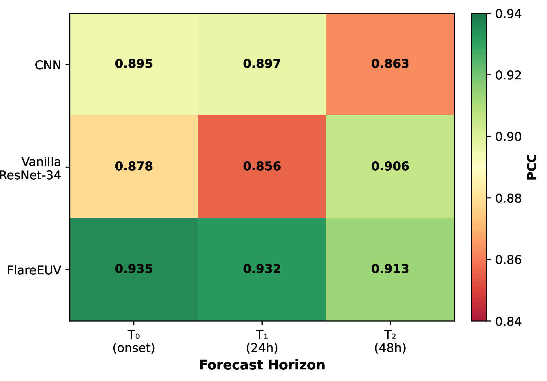
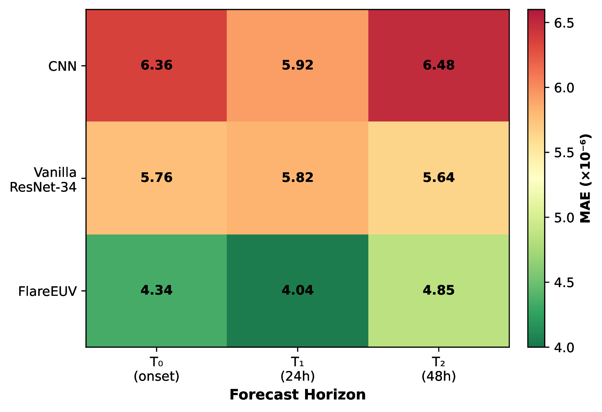
Figures 8 and 9 present per-horizon performance breakdown, revealing that FlareEUV maintains consistent advantages in all three forecast horizons. The per-horizon analysis reveals two key findings. First, FlareEUV achieves the strongest performance on all horizons, with particularly notable improvements at \(T_0\) (flare onset: PCC = 0.935, MAE = \(4.34{\times}10^{-6}\) W/m\(^2\)/nm) where accurate characterization of peak irradiance is most critical for operational forecasting. Second, Vanilla ResNet-34 shows anomalously strong performance at \(T_{2}\) (PCC = 0.906) despite weaker near-term forecasting (PCC = 0.878 at \(T_0\), PCC = 0.856 at \(T_{1}\)), suggesting that residual connections may preferentially capture long-term decay patterns even without explicit attention mechanisms. However, FlareEUV’s consistently superior performance across all horizons (PCC \(>\) 0.91 at every horizon) confirms that SE attention provides robust multi-day generalization superior to both lightweight and deep baseline architectures.
4 Conclusion↩︎
We presented the FlareEUV model, a lightweight 13-channel fusion framework to predict daily SDO/EVE 6.5 nm irradiance during significant solar flares in the period between 2011 and 2014 in Solar Cycle 24. By harmonizing AIA radiative observations with the HMI magnetic-field structure and employing a horizon-weighted regression objective, the model learns stable magnetic–radiative dependencies that generalize across diverse flare events.
Under a rigorous leave-one-flare-out (LOFO) protocol on 33 major flares, FlareEUV achieved a strong global correlation of PCC = 0.927 (p \(<10^{-40}\)) and a mean absolute error of MAE = \(4.41 \times 10^{-6}\) W/m\(^{2}\)/nm, demonstrating an accurate prediction of the magnitude of irradiance. The per-horizon analysis revealed consistently strong performance, with correlations of PCC (at \(T_{0}\)) = 0.935, PCC (at \(T_{1}\)) = 0.932 and PCC (at \(T_{2}\)) = 0.913, and corresponding mean absolute errors of MAE (at \(T_{0}\)) = \(4.34\times10^{-6}\), MAE (at \(T_{1}\)) = \(4.04\times10^{-6}\), and MAE (at \(T_{2}\)) = \(4.85\times10^{-6}\) W/m\(^{2}\)/nm. The minimal degradation from \(T_0\) to \(T_{2}\) (2.4% drop in correlation) indicates reliable multi-day forecasting capability. These results substantially outperform both single-modality baselines (AIA-only: PCC = 0.868; HMI-only: PCC = 0.835) and architectural baselines (Baseline CNN: PCC = 0.885; Vanilla ResNet-34: PCC = 0.879), confirming that the combination of multimodal fusion, deep residual architecture, and channel attention mechanisms is essential for robust cross-flare generalization. Notably, the addition of SE attention blocks adds only 43,520 parameters (+0.2% overhead) yet yields a 5.5% improvement in correlation over Vanilla ResNet-34, demonstrating the efficiency of lightweight attention mechanisms for heliophysics applications.
The FlareEUV framework is fully reproducible and establishes a compact benchmark for multi-instrument irradiance forecasting. It should be noted that, although FlareEUV was only tested on significant flares in the period between 2011 and 2014 in this study, the framework should generalize to significant flares in other periods. We chose this period to demonstrate how FlareEUV works because 2014 is solar maximum in Solar Cycle 24, with many strong active regions, significant flares and coronal mass ejections. In the future, we plan to apply FlareEUV to additional solar cycles (e.g., Solar Cycle 25), smaller flare classes, and operational real-time forecasting systems to further validate cross-cycle generalization and enable deployment in space-weather prediction infrastructure.
Acknowledgment↩︎
The authors acknowledge NASA/SDO and the EVE, AIA, and HMI instrument teams for providing open access to the data used in this study [23]–[25] as well as the SunPy project community [26] for providing Python libraries for solar physics studies. This work was supported in part by NASA under grant numbers 80NSSC24M0174 and 80NSSC24K0548.