Approximating SPR Distance Between Phylogenetic Trees with Graph Neural Networks
July 17, 2026
Abstract
Comparing phylogenetic tree topologies is essential for understanding epidemic dynamics, yet biologically meaningful distances such as the Subtree Prune and Regraft (SPR) distance are NP-hard to compute and intractable on large datasets. We investigate
whether a Graph Neural Network (GNN) can approximate SPR distances in near-constant time per comparison after training. Our contributions are fourfold. First, we build and publicly release a dataset of 864 phylogenetic trees inferred with UPGMA and
Neighbor-Joining over four bacterial species, spanning up to 9,500 isolates, together with 388 labelled tree pairs. Second, we establish a reproducible pre-processing pipeline including midpoint re-rooting, which reduces tree depth and supplies the rooting
required for exact distance computation and for the model’s root-based features. Third, we validate the supervision target: on small trees, where exact SPR is tractable, the unrooted phangorn::SPR.dist heuristic correlates almost perfectly
with the exact rooted distance computed by rspr (Pearson \(0.98\)–\(0.99\)), making it an excellent monotonic surrogate. Lastly, we train a Siamese Graph Isomorphism Network
(GIN) regressor. In-distribution, em i.e., held-out trees from the same species and size range as training, it explains roughly 87–90% of the variance (\(R^2 \approx 0.87\) on a held-out split; \(0.90 \pm 0.19\) under stratified cross-validation), with about four times lower error than a mean-predictor baseline, and shows partial transfer to unseen species (\(R^2 \approx 0.37\)). Its
main limitation is extrapolation to trees larger than those seen in training, where accuracy collapses. The released dataset and the validated heuristic versus exact relationship provide a reproducible basis for scaling learned SPR approximation.
1 Introduction↩︎
Determining the origin, evolutionary dynamics and transmission patterns of bacterial and viral epidemics is among the central challenges of computational biology. Phylogenetic inference reconstructs these evolutionary relationships. Its outcome, the phylogenetic tree [1], is an indispensable data structure for tasks such as tracking pathogen strains through an outbreak.
Different inference methods, such as Maximum Likelihood [2], Maximum Parsimony [3], Neighbor-Joining (NJ) [4], UPGMA [5], or goeBURST [6], frequently produce distinct topologies for the same isolates [7], so evaluating and reconciling them requires comparing trees at scale. The available distance measures trade speed against biological meaning (Section 2): cheap partition-based measures such as Robinson–Foulds [8] saturate quickly and overreact to a single displaced taxon, whereas the Subtree Prune and Regraft (SPR) distance [9] directly counts the prune-and-regraft operations between two topologies and so models reticulate events such as recombination and horizontal gene transfer. That biological fidelity is costly since computing the rooted SPR distance is NP-hard [10], which rules out exact computation for trees with thousands of leaves.
This motivates an approximation that is both accurate and fast. Since the exact rooted distance is intractable at scale, it cannot serve as a training signal for large trees; we therefore adopt a polynomial-time heuristic, the unrooted phangorn::SPR.dist, as the supervision target, after first verifying on small trees—where exact computation is feasible—that it tracks the exact rooted SPR distance almost perfectly (Pearson 0.98–0.99). We then ask whether a GNN [11] can learn to reproduce this surrogate directly from tree structure, so that each comparison reduces to a single forward pass at inference time. Our contributions are:
A reproducible pre-processing pipeline that slices genomic profiles into size-stratified sub-datasets, diversifies them through controlled shuffling, infers UPGMA and NJ trees, applies midpoint re-rooting [12], and extracts SPR supervision labels.
A publicly released dataset [13] of 864 trees and 388 labelled tree pairs across four bacterial species, with isolates up to 9,500 sequences.
A validation of the supervision target against the exact rooted SPR distance computed with
rspr[14], clarifying the relationship between the exact metric and thephangorn[15] heuristic.A Siamese GIN [16] regressor with training and inference pipelines1, together with an assessment of where it works (in-distribution), where transfer is partial (across species), and where it fails (size extrapolation).
2 Related Work↩︎
Molecular epidemiology and comparative genomics increasingly reconstruct phylogenies from typing and whole-genome data for collections reaching thousands of isolates, where the resulting trees drive outbreak investigation and the study of recombination
and horizontal gene transfer [1]. Because standard inference methods, such as NJ [4], UPGMA [5], goeBURST [6], Maximum Likelihood [2] and Maximum Parsimony [3], routinely return different topologies for the same isolates [7], comparing trees
is a recurring and increasingly large-scale step in any such analysis. The metric chosen for that comparison is in practice a tooling decision with biological consequences. The Robinson–Foulds distance [8] is the field’s workhorse because it is linear-time and widely implemented, but it saturates on divergent isolates and overreacts to a single misplaced taxon, limiting its use for fine-grained
outbreak resolution; information-theoretic variants soften this [17]. Quartet [18] and path-difference [19] measures recover more topological detail but report a value that
does not translate cleanly into evolutionary events. Rearrangement distances are the biologically literate alternative: the Subtree Prune and Regraft (SPR) distance [9], like the related Tree Bisection and Reconnection [20], counts the edit operations between two trees and so directly
models reticulate processes such as recombination and horizontal gene transfer. The cost is computational, since rooted SPR is NP-hard [10], and
this shapes the available software: rspr [14] delivers exact rooted distances through maximum agreement forests but only for modest
trees, whereas phangorn [15] scales by estimating the unrooted distance heuristically, with no approximation guarantee, based on the
algorithm of de Oliveira Martins et al. [21]. We address this lack of a guarantee by validating the heuristic directly against the exact rooted
distance (Section 5) before adopting it as our supervision target. A related quantity, the lower bound on the unrooted distance, is similarly tractable via agreement forests [22]. What no existing tool offers is amortized, near-constant-time comparison: exact methods do not scale, and although the heuristic scales, it must be
recomputed for every pair.
This is the gap a learned estimator can fill, and graph neural networks [11] are a natural instrument because a phylogeny is a graph. Their behaviour on this data hinges on the aggregation function: the degree-normalised mean of Graph Convolutional Networks [23] and the learned attention of Graph Attention Networks [24] tend to smooth away structure on the near-3-regular topologies of binary trees, whereas the injective sum of Graph Isomorphism Networks [16] preserves exactly the differences the SPR distance depends on, matching the discriminative power of the Weisfeiler–Lehman test.
For pairwise comparison, two paradigms dominate. Cross-graph matching networks such as Graph Matching Networks [25] inject node-to-node attention for fine-grained accuracy but scale poorly with graph size. Graph embedding approaches, exemplified by SimGNN [26], encode each graph independently and predict from the pair of embeddings; these Siamese designs [27] are cheaper and scale better. Given our target of trees with thousands of leaves, we adopt the embedding paradigm with a Siamese GIN encoder. To our knowledge, approximating the NP-hard SPR distance on rooted phylogenies with this approach has not previously been addressed.
3 Dataset and Ground-Truth Construction↩︎
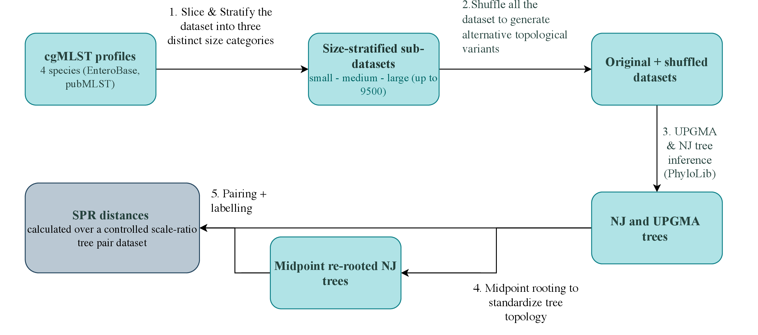
As depicted in Figure 1, the dataset is organised as a five-stage pipeline.
3.0.1 Profiles and stratification.↩︎
We sample core-genome MLST (cgMLST) [28] profiles for four bacterial species: Clostridium, Salmonella and Vibrio from EnteroBase [29], and Streptococcus pneumoniae from PubMLST [30]. A custom R script slices the original profiles sequentially, always from the first row onward, into three size tiers: small (90–1,000 isolates, 25%), medium (2,000–6,000, 25%) and large (7,000–9,500, 50%); see Fig. 2 (a). Slicing contiguously preserves the implicit temporal and geographic structure of the profiles and ensures smaller sub-datasets are nested within larger ones.
3.0.2 Controlled shuffling.↩︎
Distance-based methods such as NJ and UPGMA are sensitive to input order when breaking ties in the distance matrix. We exploit this with a seeded permutation script that reorders profile rows, forcing the algorithms to resolve ties differently and produce topologies with minor, controlled structural variations.
3.0.3 Inference and re-rooting.↩︎
From each (original and shuffled) sub-dataset we compute a Hamming distance matrix and infer UPGMA and NJ trees in Newick format with PhyloLib [31]. NJ trees are unrooted, with a basal trifurcation, so we apply midpoint rooting [12] using Biopython’s
Bio.Phylo [32]. This yields the rooted binary trees required by the exact rooted-SPR algorithm and defines the model’s root-based node
features. Rooting also balances the topology: on a 469-isolate Salmonella tree it reduced maximum topological depth from 52 to 33 and average depth from \(\approx 31.2\) to \(\approx
16.0\), which lowers the cost of the traversal-based heuristic label computation.
3.0.4 Pairing and labelling.↩︎
We form 388 tree pairs following a fixed niche distribution: UPGMA vs. NJ (40%), NJ vs.NJsh (25%), UPGMA vs. UPGMAsh (15%), and two zero-distance control blocks NJ vs.NJ and UPGMA vs.UPGMA (10% each); see Fig. 2 (b). For each pair we extract the SPR label with phangorn::SPR.dist; the structural trace (the leaves that move between the two topologies) is obtained from the maximum agreement forest (MAF) computed
exactly with rspr [14], for which the rooted SPR distance equals the number of MAF components minus one. The master table is split into
disjoint train, validation and test subsets.
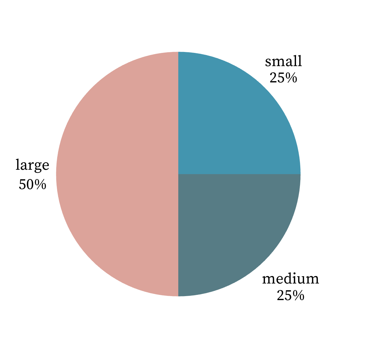
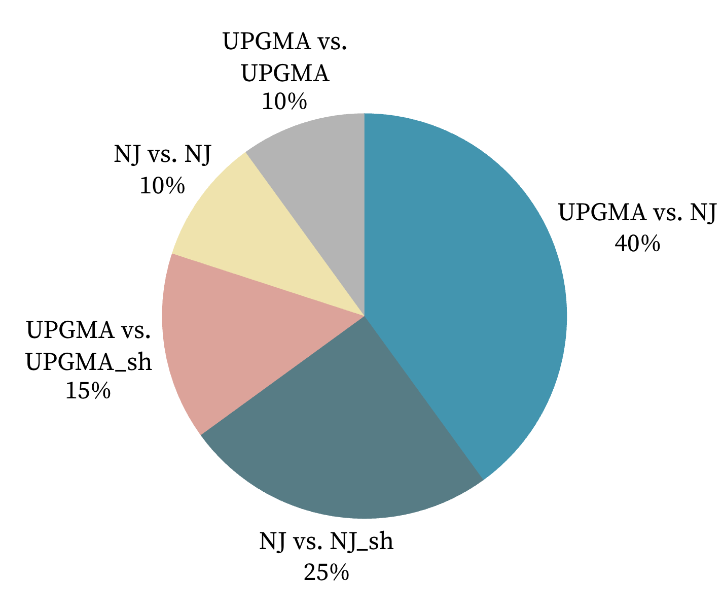
Figure 2: Dataset statistics.. a — Dataset size distribution., b — Tree pair distribution for pairing and labelling.
Notice that the supervision target is a heuristic estimate of the unrooted SPR distance, the phangorn::SPR.dist [21],
and although it was originally described as a conservative upper-bound estimate, no error bound was ever formally established, and in practice it tends to underestimate the true SPR distance when that distance is small relative to tree size, which
is precisely our regime. Second, inspection of the phangorn source shows that SPR.dist internally unroots both inputs (it calls clean_phylo(…, unroot=TRUE) and canonicalises bipartitions with
SHORTwise) and exposes no rooted option. Passing rooted trees therefore does not yield a rooted SPR distance. In contrast, rspr [14] computes the exact rooted SPR distance. The two tools thus measure related but distinct quantities. In Section 5 we evaluate how the exact rooted SPR distance compares against
the unrooted heuristic estimate from the phangorn package.
4 Method↩︎
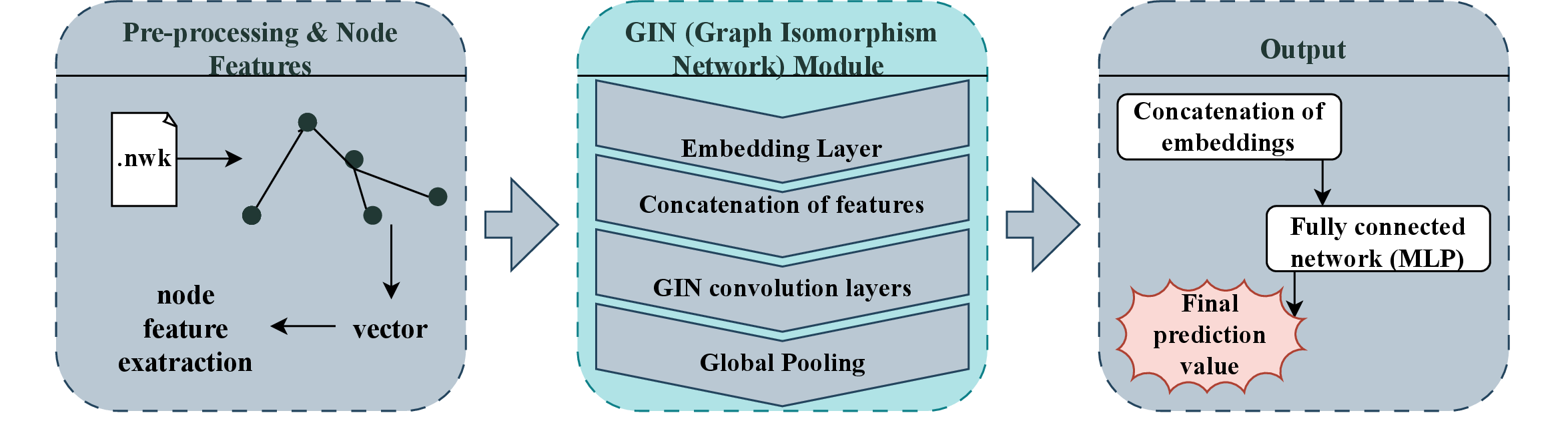
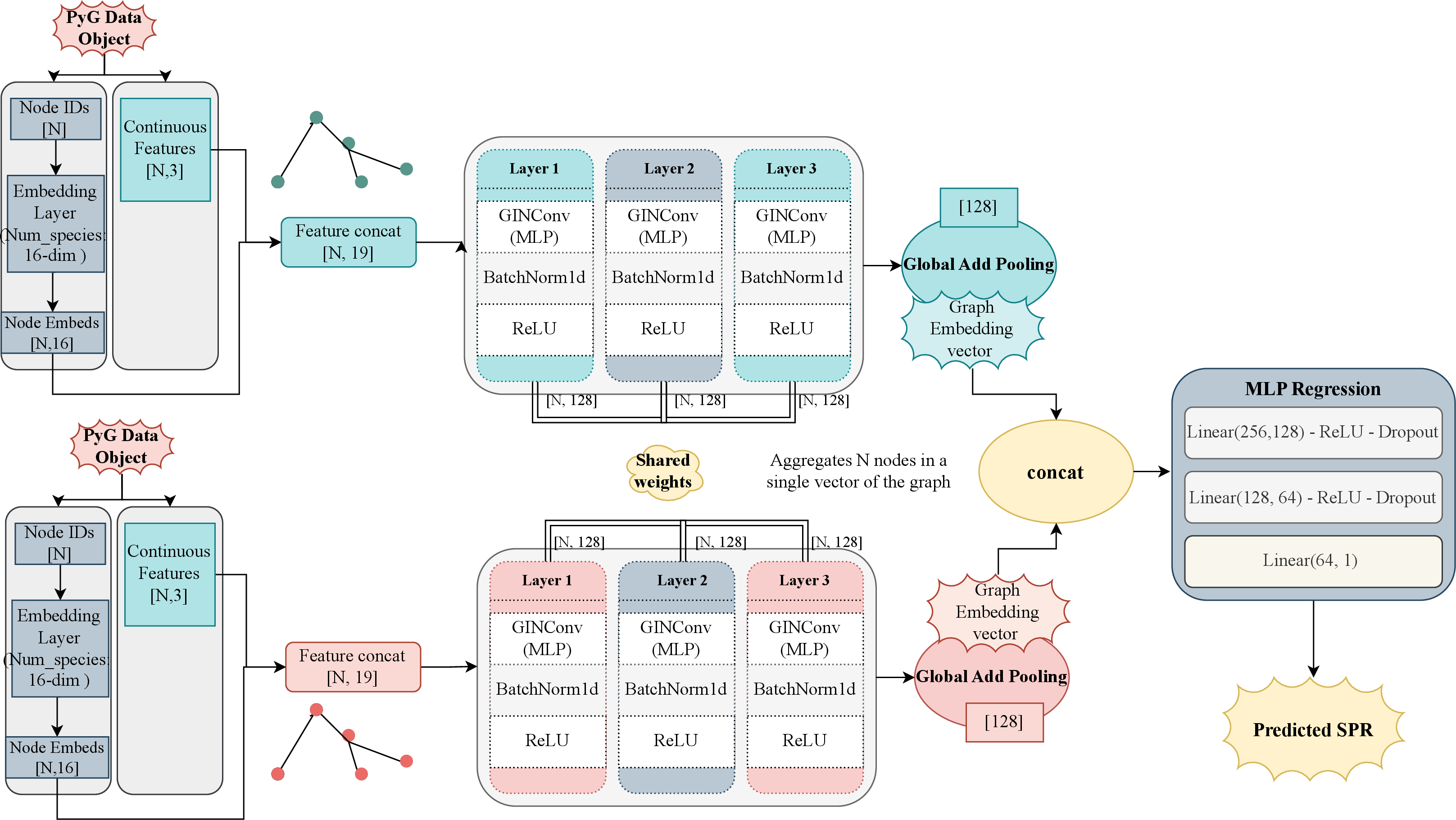
Figure 3 gives a high-level overview of the model: a tree representation module produces node features, a shared GIN module encodes each tree, and an output module pools and regresses the pair to an SPR distance.
4.1 Graph Representation and Node Features↩︎
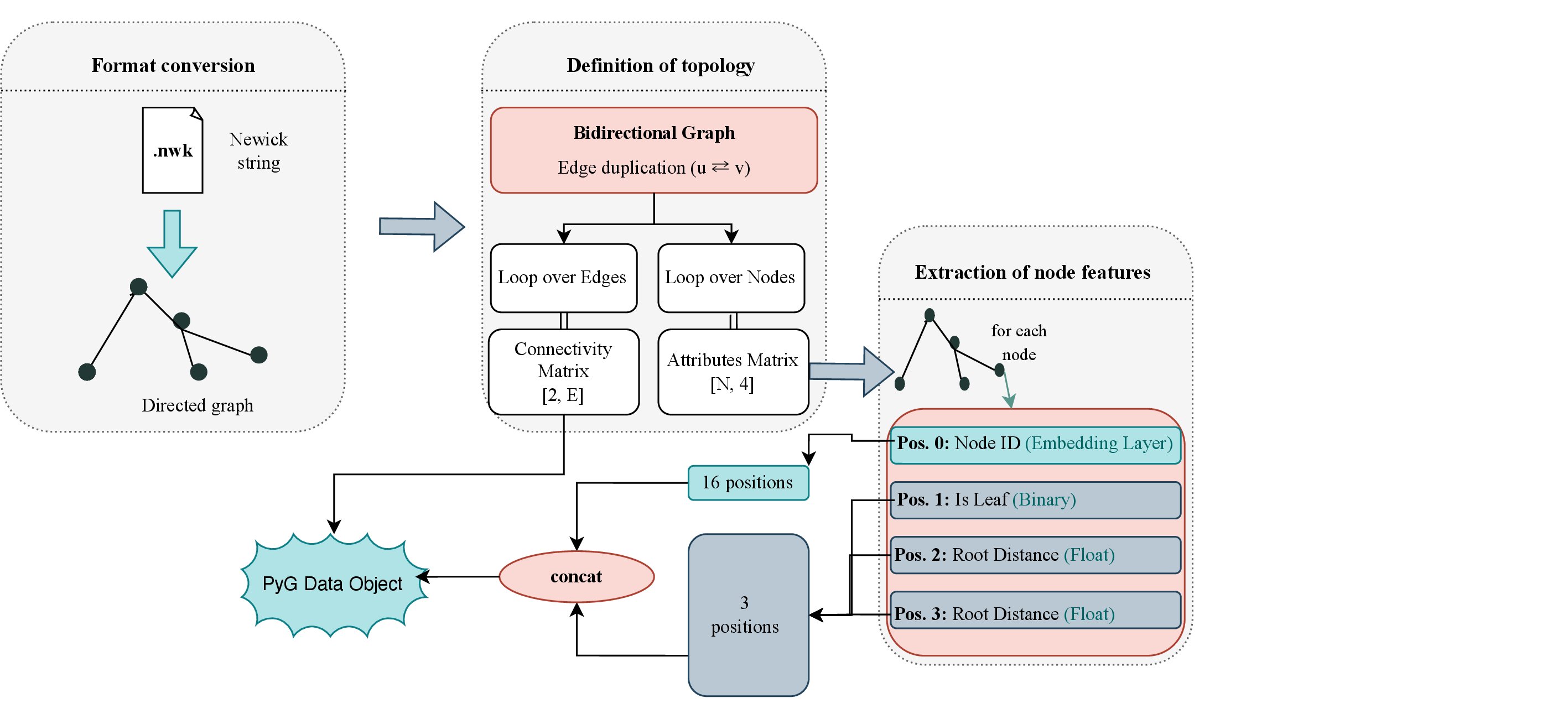
Each Newick tree is parsed with Biopython [32] and converted to a directed graph whose root is the unique in-degree-zero vertex. Then, it is encoded as
a bidirectional graph in PyTorch Geometric [33] so that messages propagate in both directions. In this context, each node carries a four-dimensional feature
vector: node degree, a binary leaf indicator, the topological distance to the root in number of branches, and a categorical taxonomic identifier. The first three are used directly, while the identifier is mapped through a trainable Embedding
layer of dimension 16, with vocabulary size set dynamically to \(\texttt{max\_id}+1\) to handle large isolate counts. Concatenation yields a 19-dimensional input per node. Figure 4
illustrates the full encoding, from the Newick string to the per-node feature vector.
4.2 Siamese GIN Regressor↩︎
The model, detailed in Fig. 5, is a Siamese embedding network: both trees of a pair pass through the same GIN encoder. Each GIN layer [16] updates node features as \[h_i^{(k)} = \mathrm{MLP}^{(k)}\!\left( (1+\epsilon^{(k)})\, h_i^{(k-1)} + \sum_{j \in \mathcal{N}(i)} h_j^{(k-1)} \right),\] where \(\mathcal{N}(i)\) is the neighbourhood of node \(i\). We stack two GIN layers of hidden dimension 128; each wraps a two-layer MLP, Linear-ReLU-Linear, followed by batch normalisation [34] and ReLU. A global sum-pooling layer then aggregates node features into a fixed-size graph embedding \[v_g = \sum_{i \in V_g} h_i .\] The two embeddings \(v_a\) and \(v_b\) are concatenated into a 256-dimensional vector and regressed by an MLP head \(256\!\to\!128\!\to\!64\!\to\!1\) with ReLU activations and dropout \(0.3\), producing the predicted SPR distance.
4.3 Training↩︎
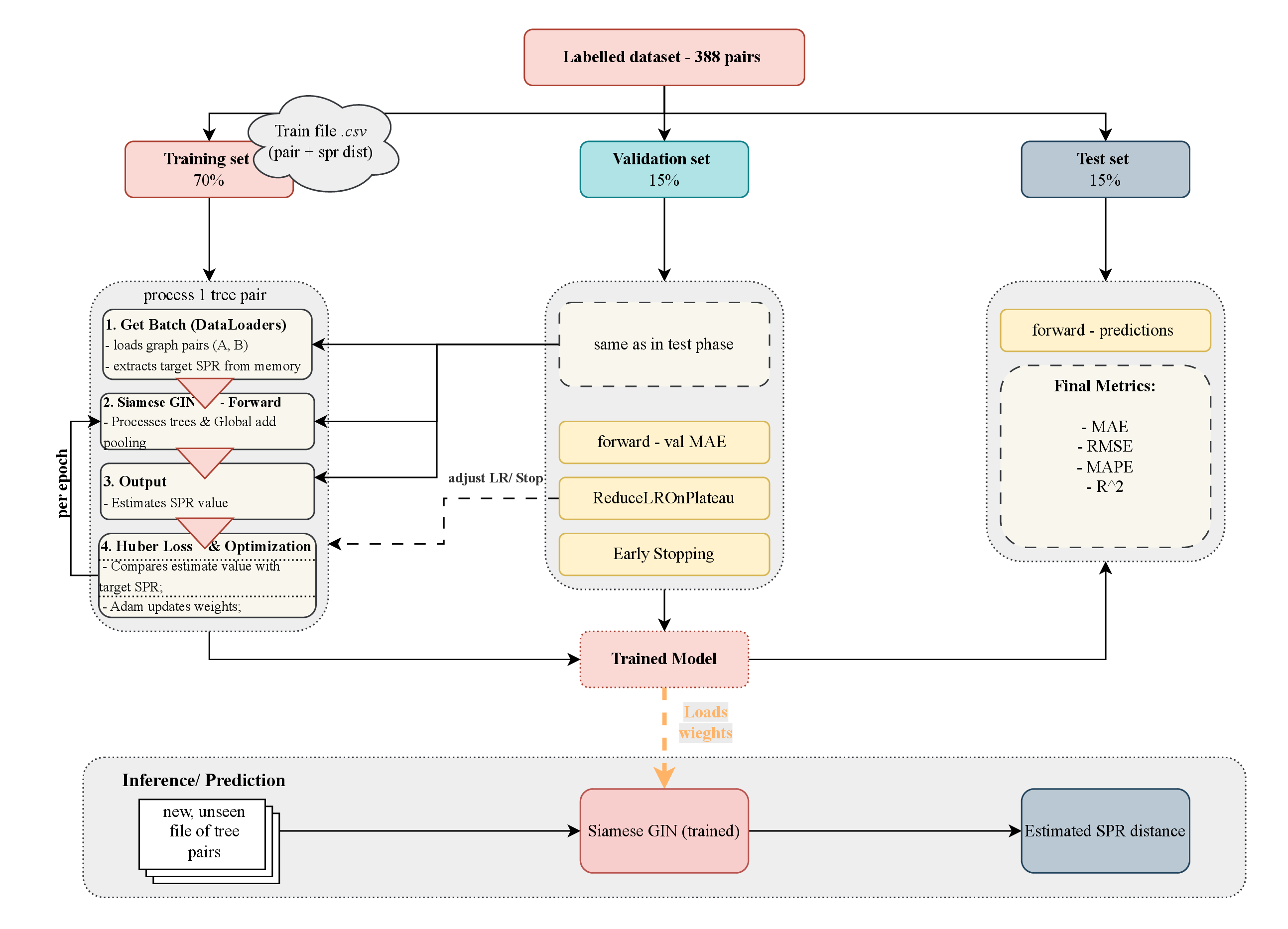
To keep training efficient, each tree is parsed and converted to a PyTorch Geometric object once and cached in memory, which reduces the per-epoch cost from \(O(\text{epochs}\times N)\) to \(O(N)\). The network is trained with the Adam optimiser [35] at a learning rate of \(10^{-4}\) and weight decay of \(10^{-4}\), minimising the Huber loss [36], which is robust to the right-skewed distribution of SPR values. The learning rate is halved on plateau after 10 epochs without improvement, and training stops early after 25 such epochs. We split the labelled pairs 70/15/15 into training, validation and test sets under a fixed seed. Predicted distances are clamped at zero, since negative distances are biologically meaningless. Performance is reported as Mean Absolute Error (MAE), Root Mean Squared Error (RMSE), Mean Absolute Percentage Error (MAPE) and the coefficient of determination \(R^2\). Figure 6 summarises the full training, validation, testing and inference workflow.
5 Experimental Evaluation↩︎
This section evaluates the approach along three axes. We first assess the scalability of the labelling pipeline; we then quantify how well the phangorn heuristic used for supervision approximates the exact rooted SPR distance; and we
finally measure the accuracy and generalization of the trained Siamese GIN across in-distribution, cross-species, and size-extrapolation regimes.
5.1 Scalability of the Pipeline↩︎
In stress testing on a virtual machine with 240 GiB of RAM and Intel Xeon Silver CPUs, the labelling pipeline scaled to trees of up to 9,500 profiles. Exact rspr computation, by contrast, was not feasible for all those trees. A trained GNN
then predicts a distance in a single forward pass, in a fraction of the heuristic’s time.
5.2 Validating the Supervision Target↩︎
On small validation trees (20–90 leaves), where exact computation is tractable, we compared the unrooted phangorn heuristic against the exact rooted SPR distance. Table 1 reports the Clostridium pairs.
The heuristic is strongly rank-correlated with the exact distance (Pearson \(0.983\) on Clostridium, \(0.9935\) on a Vibrio subset, and \(0.99\) pooled over \(n=26\) pairs), but it systematically underestimates the magnitude, returning on average about \(65\%\) for Clostridium and
\(71\%\) for Vibrio of the exact value.
| Size | Pair | Heuristic | Exact | Trace |
|---|---|---|---|---|
| 20 | NJ\(_s\) vs UPGMA\(_s\) | 6 | 9 | 15 |
| 30 | UPGMA\(_s\) vs UPGMA | 12 | 20 | 22 |
| 40 | UPGMA\(_s\) vs UPGMA | 17 | 28 | 35 |
| 45 | UPGMA vs NJ\(_s\) | 20 | 33 | 37 |
| 50 | UPGMA vs UPGMA\(_s\) | 22 | 38 | 43 |
| 55 | UPGMA vs NJ | 5 | 8 | 21 |
| 60 | UPGMA vs NJ | 5 | 9 | 22 |
| 65 | UPGMA vs NJ | 6 | 9 | 26 |
| 70 | UPGMA vs NJ | 7 | 10 | 28 |
| 75 | UPGMA vs NJ | 7 | 11 | 31 |
| 80 | UPGMA vs NJ | 10 | 14 | 33 |
| 85 | UPGMA vs NJ | 14 | 19 | 53 |
| 90 | UPGMA vs NJ | 15 | 20 | 60 |
This underestimation is expected rather than a heuristic failure, and has two sources. First, phangorn estimates the unrooted SPR distance, which is generally no larger than the rooted distance preserved by midpoint
rooting. Second, the heuristic itself carries no proven approximation bound and empirically underestimates the true SPR distance when that distance is small relative to tree size, consistent with the systematic gap we observe. Both effects push the
heuristic below the exact rooted value. The very high correlation nonetheless shows it is an excellent monotonic surrogate, which is what matters for training a regressor, even if it is a biased estimator of the rooted magnitude. The trace
(relocated leaves) is far larger than the SPR distance itself, for example 8 operations but 21 leaves moved at size 55, since a single prune-and-regraft move can displace an entire subtree.
5.3 Model Performance↩︎
Under stratified cross-validation the Siamese GIN reaches \(R^2 = 0.905 \pm 0.191\), MAE \(= 92.24 \pm 7.02\), RMSE \(= 128.14 \pm 11.07\) and MAPE \(= 2.16\% \pm 0.37\%\). The standard deviation is driven by occasional right-skewed outliers in small validation splits rather than by instability of the fit. Table 2 reports three single-split configurations that delimit the model’s operating envelope.
| Configuration | MAE | RMSE | \(R^2\) | Baseline MAE |
|---|---|---|---|---|
| In-distribution (4 species, mixed sizes) | 127.13 | 202.24 | 0.873 | 485.78 |
| Cross-species (train 2 sp./ test 2 sp.) | 208.70 | 325.72 | 0.368 | 406.05 |
| Size extrapolation (small+med.\(\to\) large) | 375.90 | 643.02 | \(-0.14\) | 553.65 |
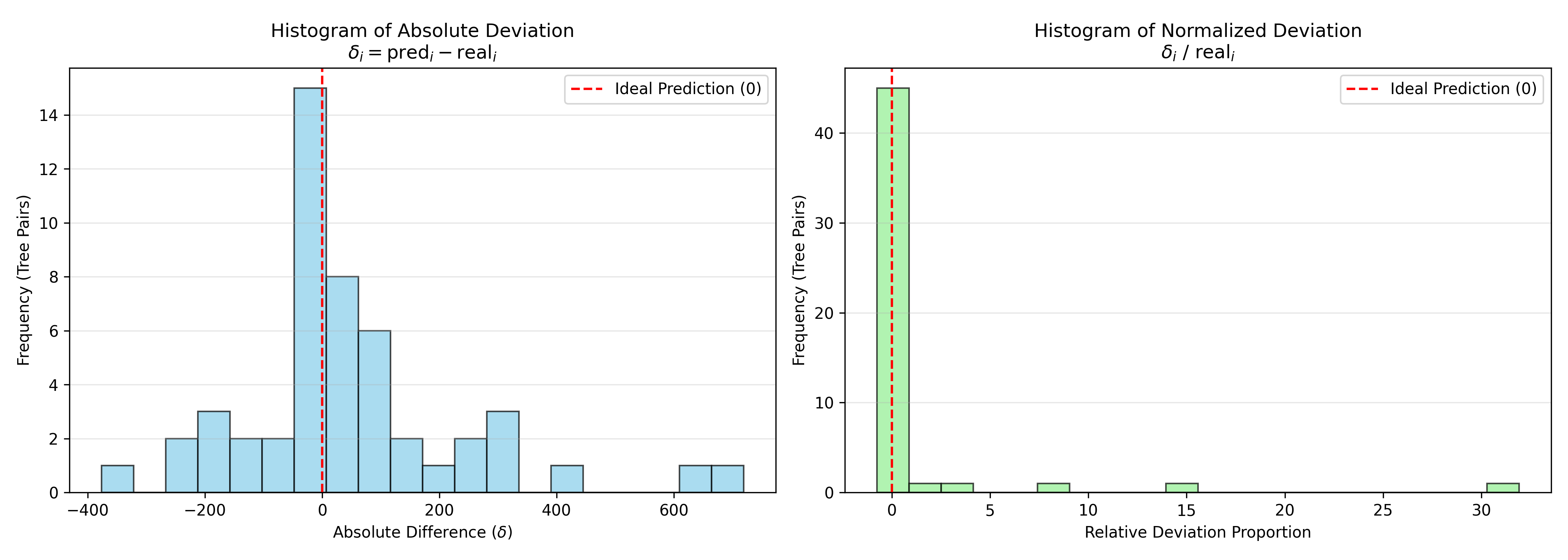
Three findings stand out. (i) In-distribution, the model explains \(\approx 87\%\) of the variance and beats the mean baseline by roughly \(4\times\) in MAE, so the GNN genuinely learns to compare topologies. (ii) Trained on two species and tested on two unseen ones (Clostridium and Vibrio \(\to\) Salmonella and S. pneumoniae), it attains \(R^2 = 0.37\). This indicates that the learned representation captures some species-agnostic structure, but that cross-species generalization remains challenging. The drop is hard to attribute to domain shift alone, since this split also reduces the training set substantially, so data scarcity is a likely contributing factor. (iii) When trained only on small and medium trees and asked to predict on large ones, performance falls below the mean baseline (\(R^2 = -0.137\)): the model does not extrapolate to tree sizes outside its training range. The calibration analysis on the in-distribution test set, shown in Figure 7, is consistent with this: predictions cluster around the ideal \(y=x\) line but compress towards the mean, overestimating short distances and underestimating long ones. Figure 8 refines this picture through the deviation histograms. The absolute-deviation histogram concentrates sharply around zero, so the model predicts most pairs accurately, with a slight right-skew and a tail that indicate an occasional tendency to overestimate on complex topologies. The normalized-deviation histogram is likewise concentrated near zero, showing that the largest absolute errors fall on pairs with inherently large SPR distances, so the relative error stays low across most of the domain.

5.4 Discussion↩︎
Taken together, the experiments show that the binding limitation is neither the architecture nor, primarily, the absolute size of the labelled set (388 pairs), but its coverage across tree scales. The model interpolates well and transfers only partially across species, but it cannot yet extrapolate in size, and it inherits a calibration bias from the heuristic labels and from sum pooling. These limitations are addressable: enriching the training distribution with larger trees, exploring size-aware normalisation, and correcting the label offset are concrete next steps. Among the pooling strategies we tested, sum pooling gave the best overall results, but it remains a source of the size-related bias, so alternative aggregation schemes are worth exploring.
6 Final Remarks↩︎
We presented a reproducible ecosystem for approximating the NP-hard SPR distance between phylogenetic trees: a pre-processing pipeline, an openly released dataset of 864 trees and 388 labelled pairs, and a Siamese GIN regressor with training and
inference tools. We validated the supervision target against exact rooted SPR (Pearson \(0.98\)–\(0.99\)) and clarified the distinction between phangorn and rspr.
The model predicts SPR distances accurately in-distribution (\(R^2 \approx 0.87\)–\(0.90\)) and shows partial transfer across species (\(R^2 \approx 0.37\)),
while its current weakness is size extrapolation. Future work will expand the dataset towards larger topologies, add size-aware pooling and calibration, and benchmark the learned predictor against exact and approximate SPR tools.
A further direction is to predict the SPR trace rather than only its magnitude: to identify the specific leaves that must be relocated to transform one tree into the other, recovering the sequence of prune-and-regraft operations relating the
two topologies. This would let the model report not only how far apart two trees are but where they differ. The trace currently depends on exact MAF extraction via rspr, whose cost grows prohibitive on large trees, so trace
supervision at scale would itself require a heuristic or learned approximation of the MAF. Together, these steps target a fast, scalable approximation suitable for large-scale epidemiological and comparative-genomic analyses.
6.0.1 ↩︎
The authors acknowledge the support by national funds through the Fundação para a Ciência e a Tecnologia, I.P.(FCT) under projects UID/50021/2025, UID/PRR/50021/2025, UID/PRR/00006/2025, and grant 2023.17447.ICDT.
6.0.2 ↩︎
The authors have no competing interests to declare that are relevant to the content of this article.