Disentangling Forced and Internal Climate Variability in Single Realizations using Dynamic Mode Decomposition with Control
July 13, 2026
1 Introduction↩︎
Observed climate change reflects the superposition of two contributions: the response of the climate system to external forcing (e.g., greenhouse gases, aerosols, and volcanic and solar activity) and internal variability generated by its own coupled dynamics [1], [2]. The forced response drives the long-term trends behind the rising frequency and intensity of many climate extremes, whereas internal variability modulates these trends across time scales from seasons to decades and dominates the uncertainty of near-term, regional projections [2], [3]. Accurately disentangling the two is therefore fundamental both to attributing observed changes to human influence and to producing credible, policy-relevant projections [4], [5].
However, we observe only a single realization of Earth’s climate, in which forced and internal contributions are superposed, meaning controlled experimentation over the observational record is inherently impossible. This fundamental limitation motivates the development of Earth system models (ESMs), which enable the simulation of multiple realizations of the climate system under varied forcing scenarios and initial conditions, now routinely run as initial-condition large ensembles [6]–[8]. Under time-dependent forcing, the climate as a dynamical system is naturally described by a pullback (or snapshot) attractor, approximated by evolving a large ensemble of trajectories from different initial conditions under identical forcing until initial-condition dependence decays [9]–[14]. The resulting time-dependent collection of states defines the instantaneous climate statistics. Its ensemble mean could be used as a definition of a forced response, and deviations around the mean would then represent internal variability (see Section 2). This framework generalizes naturally to non-stationary climates and underlies the standard ensemble-mean definition of forced response in large ensembles [15].
Yet to disentangle forced response and internal variability in the observational record, we must develop methods to estimate these components from a single realization of the climate system. A wide range of approaches has been proposed for this task, spanning statistical detection and attribution methods [5] to dynamical systems-based techniques [16], [17]. Many of these methods are supervised by ESM ensembles, meaning they directly use the ensemble-mean “ground truth” forced response in ESMs and sometimes ESM simulations. For example, supervised methods include fingerprinting [5], [18]–[21], which can be extended to nonlinear settings using neural networks [22]–[24], as well as dynamical adjustment [25]–[27], which removes the influence of atmospheric circulation variability by using ESM-derived analogs. Although these methods can be skillful, they often require substantial computational resources, can reduce physical interpretability, and depend on the fidelity of the underlying ESM ensemble in representing the real climate and its forced response.
Linear, unsupervised statistical machine learning (ML) methods have been highly studied and are simple, admit fast computation times for large-scale experimentation, and retain high physical interpretability. They include dynamical system models [16], [17], [28] such as linear inverse models (LIM) [29], regression-based approaches such as global mean temperature regression [30], and decomposition methods such as low frequency component analysis (LFCA) [31] or linear dynamical modes (LDMs) [32], both benefitting from the smoothness of the underlying principal components.
The recent Forced Component Estimation Statistical Method Intercomparison Project (ForceSMIP) delivered the first large-scale, common-protocol comparison of this zoo of statistical forced-response estimators [21]. Among the unsupervised single-realization methods appearing in ForceSMIP, some focus on separating forced response and internal variability using dynamical system models [16], ignoring forcing information; others use regression with forcing information [30], thereby missing climate system dynamics. Non-autonomous (forced) dynamical system models are the natural way to bridge this gap, since they let the evolution operator itself depend on the external forcing [33]–[35]. Despite being actively developed and used in climate studies [36]–[41], they have not been widely applied for forced response and internal variability identification. The simplest linear version is used in dynamic mode decomposition with control (DMDc) [42], which augments a linear dynamical system with an external control term. However, DMDc alone does not address the problem of forced response and internal variability disentanglement.
Here we introduce PullbackDMDc, a simple, interpretable, unsupervised linear method that turns this idea into a forced/internal decomposition. We view a single climate record as lying on the pullback attractor of a linear stochastic system driven by external forcing. Because the system is linear, its pullback attractor collapses to a single trajectory that splits exactly into a forced response, controlled by the forcing, and an internal component, driven by noise, both read directly off the fitted linear evolution matrices. This links pullback-attractor theory with data-driven modelling and, by projecting onto the DMDc eigenmodes, expresses the full spatio-temporal record as a sum of spatial patterns, each carrying its own forced and internal time series.
We evaluate the method across four large ensembles and reanalysis data using standard forced-response metrics. We show that PullbackDMDc achieves competitive or superior performance compared with existing methods while retaining a physically interpretable decomposition into spatial modes and their associated forced and internal components. We further show that the implied decomposition enables a diagnostic analysis and evaluation of ESMs against observations in terms of the dominant modes. We present selected examples of such an evaluation, highlighting the differences and similarities in the representation of dominant interannual-to-multidecadal modes and seasonal cycle non-stationarity across ESMs and observations.
The remainder of the paper is organized as follows. Section 2 of this paper presents the baseline methods briefly and PullbackDMDc in detail. Section 3 presents the results of forced-response estimation across all methods and ESMs, and an example of ESM evaluation using the decomposition proposed by PullbackDMDc. Find technical details and additional results in the Supplementary material.
2 Methods↩︎
Suppose we have a time series of a climate variable at times \(t=1,2,\ldots,T\), denoted \(\{\boldsymbol{x}(1),\boldsymbol{x}(2),\ldots,\boldsymbol{x}(T)\} \subset \mathbb{R}^{M}\), with \(M\) being the number of spatial locations or the dimension of the feature space. We aim to estimate an additive forced component \(\boldsymbol{x}^{(f)}(t)\) from a time series of this single variable. The forced component represents the part of climate dynamics that responds to external forcings such as greenhouse gas emissions and aerosols. In many climate studies, it is estimated for a given ESM by taking an ensemble mean over a large number of ESM runs under the same forcing [21] or by approximating it from a smaller ensemble size [43]–[45]. This forced response approximation implicitly assumes that the ensemble mean converges to the limit \(\boldsymbol{x}^{(f)}(t)\) as the number of realizations (a.k.a. ensemble members) and the evolution time before \(t\) both go to infinity. Then the internal component \(\boldsymbol{x}^{(i)}(t)\) can be defined as a residual, so that \(\boldsymbol{x}(t)=\boldsymbol{x}^{(f)}(t)+\boldsymbol{x}^{(i)}(t)\).
Note that in this ensemble-mean definition, the independence between the forced and internal components is not guaranteed. In fact, a rigorous definition of the forced response in an arbitrary nonlinear dynamical system is not readily available. For example, \(\boldsymbol{x}^{(f)}(t)\) can miss changes in the distribution under external forcing, including climate extremes, leading to the appearance of these changes in the internal component. Still, the ensemble mean definition estimates an additive effect attributable to the forcing in a given variable, and we use it as a ground-truth definition following [21].
2.1 Baselines for forced response estimation↩︎
Our four baselines either ignore external forcing predictors, ranging from a simple global mean surface air temperature regression to linear dynamical system models, or use forcing predictors without modeling the dynamics (e.g., linear regression), two complementary limitations that PullbackDMDc is designed to overcome.
The first baseline, RegGMST [30], assumes that the global mean surface air temperature (GMST) is a good proxy for the forced response. Specifically, RegGMST is the regression of the climate signal on the mean-centered GMST time series \(\mu_{\mathrm{SAT}}(t)\). Thus we fit regression coefficients \(\boldsymbol{\beta}\) using \(\boldsymbol{x}(t) \approx \boldsymbol{\beta} \mu_{\mathrm{SAT}}(t)\), then estimate the forced response using \(\boldsymbol{x}_f(t) = \boldsymbol{\beta} \mu_{\mathrm{SAT}}(t)\). RegGMST does not model the dynamics of the climate system nor make any dynamical assumptions on the forced response.
In the Linear Inverse Model (LIM) [29], [46], we assume the time series comes from a low-dimensional stochastic dynamical system [47] with system matrix \(\boldsymbol{L}\) and noise term \(\boldsymbol{\eta}(t)\): \[\label{eq:32lim95continuous} \frac{d \boldsymbol{x}(t)}{dt} = \boldsymbol{L}\boldsymbol{x}(t) + \boldsymbol{\eta}(t).\tag{1}\] For a discrete timestep \(\tau = 1\), the \(1\)-step solution to this system can be written as \[\label{eq:32lim95discrete} \boldsymbol{x}(t) = \boldsymbol{A}\boldsymbol{x}(t-1) + \boldsymbol{\xi}(t).\tag{2}\] It is assumed that \(\boldsymbol{\xi}(t)\) is temporally white Gaussian noise with zero mean and constant covariance matrix. In this setting, jointly maximizing the Gaussian likelihood over \(\boldsymbol{A}\) and the noise covariance matrix yields the same estimate of \(\boldsymbol{A}\) as ordinary least squares. The dynamic mode decomposition (DMD) [48] method is essentially the deterministic component of a discrete-time LIM, which includes an eigendecomposition of \(\boldsymbol{A}= \boldsymbol{W} \boldsymbol{\Lambda}\boldsymbol{W}^{-1}\). See the Supplementary for the details of DMD.
LIM estimates the forced response as the data projected onto the least damped mode, that is, the eigenvector of \(\boldsymbol{A}\) with the longest decay time [16], [49]. LIM is a primitive, dynamical-system-based forced-response estimator that often produces noisy estimates.
To combat noisy forced response estimates, LIM with optimal perturbation patterns (LIMopt) yields a smoother estimate of the forced response by evolving the patterns in \(\boldsymbol{A}\) over an optimal perturbation time of \(\tau_e\) [16], [43], [50]. Using the same \(\boldsymbol{A}\) as LIM, LIMopt also seeks a smoother, least-damped pattern from \(\boldsymbol{A}\). This is done by taking the singular value decomposition (SVD) of \(\boldsymbol{A}\) after evolving it over \(\tau_e\) time steps, yielding \(\boldsymbol{A}^{\tau_e}\). Then, it uses the singular vectors associated with the largest singular value of \(\boldsymbol{A}^{\tau_e}\) to compute the forced response (see the Supplementary for further details).
In RegGMST, LIM and LIMopt, the forced component is estimated solely from the time series of the climate variable, without directly incorporating any information about external forcing. In the Linear Regression (LR) baseline, we directly estimate the forced component using external forcing information. Importantly, it assumes that there is an external forcing estimator \(\boldsymbol{y}(t)\) beyond the time series \(\boldsymbol{x}(t)\). LR does a regression on the forcing signal \(\boldsymbol{y}(t)\), fitting coefficients \(\boldsymbol{B}\) using \(\boldsymbol{x}(t) \approx \boldsymbol{B} \boldsymbol{y}(t)\), then estimates the forced response using \(\boldsymbol{x}^{(f)}(t) = \boldsymbol{B} \boldsymbol{y}(t)\).
2.2 Pullback DMDc↩︎
PullbackDMDc unifies two concepts from our baselines: it embeds the external forcing inside a LIM-type dynamical model through a linear stochastic model with forcing. Interpreting the observed climate trajectory as the pullback attractor of this model then yields a separation of forced and internal components from a single realization. We use this to extend DMDc [42] by projecting the forced and internal components onto the DMDc modes, yielding a representation of the full spatiotemporal data cube as a sum of dynamic modes, each accompanied by its own forced and internal time series.
2.2.1 Linear stochastic model with forcing↩︎
In a forced1 (driven) dynamical system framework, the evolution operator is assumed to depend directly on the external forcing signal \(\boldsymbol{y}(t)\) [33]–[35]. The simplest extension of discrete LIM 2 can be done by including a linear forcing term \(\boldsymbol{B}\boldsymbol{y}(t)\) as: \[\label{eq:32linear95system} \boldsymbol{x}(t) = \boldsymbol{A}\boldsymbol{x}(t-1) + \boldsymbol{B} \boldsymbol{y}(t) + \boldsymbol{\xi}(t).\tag{3}\] The matrices \(\boldsymbol{A}\) and \(\boldsymbol{B}\) in 3 are obtained similarly to LIM using a least-squares method without any regularization (see the Supplementary). We proceed with forced/internal component estimation for this simple model.
We interpret \(\boldsymbol{A}\) as the dynamical core of a linear stochastic emulator 3 , which defines the response of the model to non-autonomous components, such as external forcing and stochastic perturbations. Given \(\boldsymbol{B}=\boldsymbol{0}\) or \(\boldsymbol{y}(t)=\boldsymbol{0}\), this system becomes LIM and generates a stationary stochastic process with the time scales defined by the eigenvalues of \(\boldsymbol{A}\), which we call internal variability. The observed internal variability is thus related to a specific realization \(\boldsymbol{\xi}(t)\) which can be known a posteriori. On the other hand, the deterministic part corresponding to \(\boldsymbol{\xi}(t)=\boldsymbol{0}\) is commonly analyzed in DMDc studies [42], which we extend below to infer the forced and internal components. Finally, the model 3 includes a linear regression solution as a possible case \(\boldsymbol{A}=\boldsymbol{0}\).
A simple linear form of the model allows us to solve the system dynamics explicitly. Given the initial condition \(\boldsymbol{x}_{0}\) at some moment \(t_0\), the solution for the system at time \(t\) after \(t-t_0\) steps is obtained by iteratively applying 3 : \[\label{eq:solve-ds} \boldsymbol{x}(t| \boldsymbol{x}_0,t_0) = \boldsymbol{A}^{t-t_0} \boldsymbol{x}_{0} + \sum\limits_{j=0}^{t-t_0-1} \boldsymbol{A}^{j}\boldsymbol{B} \boldsymbol{y}(t-j) + \boldsymbol{A}^{j}\boldsymbol{\xi}(t- j).\tag{4}\]
2.2.2 Pullback attractor of the model↩︎
The pullback attractor [10], [51], [52] extends the well-known definition of an attractor of a deterministic dynamical system to a non-autonomous (e.g., forced) case. In an autonomous dynamical system, an attractor is a limit set of states that can be reached after forgetting the initial conditions. An attractor is not a function of time. A pullback attractor is defined for a non-autonomous system as a time-dependent family of limit sets: for each time moment \(t\), it represents a limit set achievable by the system after forgetting initial conditions, but under the same non-autonomous changes preceding the time \(t\), and thus it includes information about transient behavior in response to these changes.
Omitting a full mathematical definition, we estimate the pullback attractor for our linear stochastic model 3 . To do so, we fix the time series of non-autonomous changes to our model (i.e., external forcing \(\boldsymbol{y}(t)\) and the stochastic perturbation \(\xi(t)\)), and then take the limit by “pulling” time \(t_0\) back to \(-\infty\): \[\begin{align} \begin{aligned}\label{eq:decompose95ds} \boldsymbol{x}(t| \boldsymbol{x}_0,t_0) \underset{t_0 \to -\infty}{\xrightarrow{}} &\underbrace{\sum\limits_{j=0}^{\infty} \boldsymbol{A}^{j}\boldsymbol{B} \boldsymbol{y}(t-j)}_{\text{forced response}} + \underbrace{\sum\limits_{j=0}^{\infty} \boldsymbol{A}^{j}\boldsymbol{\xi}(t-j)}_{\text{internal variability}}\\ &= \boldsymbol{x}^{(f)}(t) +\boldsymbol{x}^{(i)}(t). \end{aligned} \end{align}\tag{5}\] Assuming that the stochastic model is globally stable, e.g., the magnitudes of the eigenvalues of \(\boldsymbol{A}\) are strictly less than \(1\), the first term in Eq. 4 disappears. So, the limit in 5 at each time \(t\) does not depend on the initial condition \(\boldsymbol{x}_0\) and consists of only one point. Thus, the pullback attractor of our system is a single trajectory. It has a simple interpretation: the system dynamics after forgetting the initial condition are uniquely determined by the non-autonomous signals \(\boldsymbol{y}(t)\) and \(\xi(t)\) and are nothing more than a solution to a non-autonomous linear equation, analogous to a linear ordinary differential equation. Intuitively, each term is the system’s fading memory of its drivers: the forced response is the forcing history \(\boldsymbol{y}\) passed through the decaying filter \(\sum_{j\ge 0}\boldsymbol{A}^{j}\boldsymbol{B}\,(\cdot)\), and internal variability is the same filter applied to the noise history \(\boldsymbol{\xi}\). Slowly decaying modes of \(\boldsymbol{A}\) retain a longer memory and therefore dominate both terms.
This linear form thus allows separation of the pullback attractor into two components: the forced response as a function of \(\boldsymbol{y}(t)\) and the internal variability driven by \(\xi(t)\) (see 5 ). Note that for a nonlinear dynamical system, the pullback attractor is a limit set and is neither a single trajectory nor admits an obvious separation of forced and internal contributions. This could pose challenges for interpreting nonlinear extensions of PullbackDMDc.
To estimate the linear forced and internal terms in practice, we assume that the observational dataset represents the dynamics of the pullback attractor, i.e., the initial conditions of the original system are forgotten. This is reasonable for climate data from reanalysis because the climate system has been naturally forced over the past millions of years and has been forced by humans since the beginning of the industrial era in the \(1800\)’s [53]. Our assumption also holds for ESM simulations, since they are typically initiated after a spin-up phase to bring the system closer to the attractor [54]. This means that we can estimate the forced response \(\boldsymbol{x}^{(f)}(t)\) and internal variability \(\boldsymbol{x}^{(i)}(t)\) by subtracting the forced response from the full data.2
Next, we estimate the forced response as the first term in 5 . This is exactly the pullback attractor of the deterministic part of the model 3 . As with standard attractor estimation, in practice, we cannot run an infinite number of evolution steps, which would yield an infinite sum. Instead, we choose an initial moment in the past, \(t_0\), that is sufficiently far from the target time interval, so that it far exceeds all exponential decay times in the matrix \(\boldsymbol{A}\) (this condition is satisfied for all examples shown in this paper). This ensures that any errors related to the initial condition are far smaller than machine precision. Then we initialize the system at \(t_0\) and run the deterministic part of 3 . After enough time steps, we obtain system states that are close to the forced response in 5 up to machine precision. It is essential that, beyond the matrices \(\boldsymbol{A}\) and \(\boldsymbol{B}\) obtained from training, this procedure requires a sufficiently long history of forcing data \(\boldsymbol{y}(t)\). If these data are not available, one would have to extrapolate \(\boldsymbol{y}(t)\) into the past, which would decrease the accuracy. Estimation of \(\boldsymbol{A}\) and \(\boldsymbol{B}\), along with the estimation of the pullback attractor forced response, is summarized in Algorithm [alg:algorithm1].
2.2.3 Data Decomposition↩︎
The matrix \(\boldsymbol{A}\) in the deterministic part of both 2 and 3 can be analyzed in terms of the complex eigendecomposition \(\boldsymbol{A}\boldsymbol{W} = \boldsymbol{W} \boldsymbol{\Lambda}\). Assuming \(\boldsymbol{A}\) is diagonalizable, we have \(\boldsymbol{A}= \boldsymbol{W} \boldsymbol{\Lambda} \boldsymbol{W}^{-1}\). This analysis is at the core of the DMD framework for autonomous models [55] and of DMDc for non-autonomous models [42], and it typically omits the model’s stochastic component.
Note that, in general, \(\boldsymbol{A}\) may not be diagonalizable. One workaround is to approximate \(\boldsymbol{W}^{-1}\) via numerical solvers for systems of linear equations. Another option, if, as in our case, \(\boldsymbol{x}(t)\) represents PCs, is to truncate the number of PCs to ensure diagonalizability.
2.2.3.1 DMDc: Spatial Modes and Timescales
The eigenvectors \(\boldsymbol{w}_1,\ldots,\boldsymbol{w}_K\) of \(\boldsymbol{W}\) are called dynamic modes, because they define the basis structures (spatial patterns, in case of spatially distributed data) which appear in the model dynamics. Since PCA is commonly used for dimensionality reduction in preprocessing, the dynamic modes are really the patterns in the original space. Specifically, \(\boldsymbol{U}\boldsymbol{w}_k\), where the columns of \(\boldsymbol{U}\) are empirical orthogonal functions of the input data.
The evolution of these dynamic modes has distinct decay times and oscillation frequencies encoded in the complex eigenvalues \(\lambda_{k}\) on the diagonal of the matrix \(\boldsymbol{\Lambda}\): \[\label{eq:32eigenvalues} \lambda_k = r_k e^{i\theta_k} \text{ where } r_k= |\lambda_k|,\quad \theta_k = {\arg\lambda_k} .\tag{6}\] Specifically, the decay time of \(\boldsymbol{w}_k\) is \(T_k = -\frac{1}{\log{r_k}}\) and the oscillation frequency is \(f_k = \frac{\theta_k}{2\pi}\), both measured with respect to the evolution time step size \(\tau\) of the operator \(\boldsymbol{A}\). The dynamic modes with the largest decay times represent the longest-lived structures, which are therefore dominant in the model dynamics and are the objects of interest and interpretation.
2.2.3.2 PullbackDMDc: Forced and Internal Components
Here we propose projecting the observational data onto the basis of dynamic modes, which includes separating forced and internal dynamics as defined in the previous section and also yields a complete data decomposition into a set of patterns and time series. First, the projection of the full data into the basis of dynamic modes is defined as a complex time series: \[\label{eq-z} \boldsymbol{z}(t) = \boldsymbol{W}^{-1} \boldsymbol{x}(t).\tag{7}\] Next, by inserting pullback attractor 5 into 7 , the projected time series for all modes decomposed into internal and forced components is \[\label{eq:z-decompose-ds} \boldsymbol{z}(t) = \boldsymbol{W}^{-1} \boldsymbol{x}^{(f)}(t)+\boldsymbol{W}^{-1} \boldsymbol{x}^{(i)}(t) = \boldsymbol{z}^{(f)}(t) +\boldsymbol{z}^{(i)}(t).\tag{8}\] It is easy to see that this change of variables results in the model: \[\label{eq:z-model} \boldsymbol{z}(t)=\boldsymbol{\Lambda}\boldsymbol{z}(t-1)+\hat{\boldsymbol{y}}(t-1)+\hat{\boldsymbol{\xi}}(t-1),\tag{9}\] with \(\hat{\boldsymbol{y}}(t)=\boldsymbol{W}^{-1} \boldsymbol{B} \boldsymbol{y}(t)\) and \(\hat{\boldsymbol{\xi}}(t)=\boldsymbol{W}^{-1}\boldsymbol{\xi}(t)\). The terms \(\boldsymbol{z}^{(f)}(t)\) and \(\boldsymbol{z}^{(i)}(t)\) represent the pullback attractor projected to the space of dynamic modes, and also correspond to the pullback attractor of the model 9 . Similarly to classic deterministic DMD modes, the evolution of each component of the pullback attractor is determined by its eigenvalue \(\lambda_k\) and the forcing/noise signals (cf. 5 ): \[\label{eq:zk-decompose-ds} z_k(t) = \sum\limits_{j=0}^{\infty} \lambda_k^{j}\hat{y}_k(t-j) + \sum\limits_{j=0}^{\infty} \lambda_k^{j}\hat{\xi}(t-j)\;= \; \boldsymbol{z}^{(f)}_k(t) +\boldsymbol{z}^{(i)}_k(t).\tag{10}\] This extends the interpretation of the DMDc of the pullback attractor solution. In practice, however, we only need the equation 8 to compute the temporal components (see the last part of the Algorithm [alg:algorithm1]).
system states \(\boldsymbol{x}(s+1), \boldsymbol{x}(2), \dots, \boldsymbol{x}(T)\), forcings \(\boldsymbol{y}(1), \boldsymbol{y}(2), \dots, \boldsymbol{y}(T)\)
\(\boldsymbol{A}, \boldsymbol{B} = \underset{\boldsymbol{A}, \boldsymbol{B}}{\mathrm{argmin}} \sum_{t=s+2}^{T} \left\|\,\boldsymbol{A}\boldsymbol{x}(t-1) + \boldsymbol{B} \boldsymbol{y}(t) - \boldsymbol{x}(t)\,\right\|_2^2\)
\(\hat{\boldsymbol{x}}_0 = \boldsymbol{0}\)
\(\hat{\boldsymbol{x}}_j = \boldsymbol{A}\,\hat{\boldsymbol{x}}_{j-1} + \boldsymbol{B}\,\boldsymbol{y}(j)\)
\(\boldsymbol{\Lambda},\,\boldsymbol{W} = \text{eig}(\boldsymbol{A})\)
\(\hat{\boldsymbol{X}}_f = [\hat{\boldsymbol{x}}_{s+1}, \hat{\boldsymbol{x}}_{s+2}, \dots, \hat{\boldsymbol{x}}_T]\)
\(\boldsymbol{X}= [\boldsymbol{x}(s+1), \boldsymbol{x}(s+2), \dots, \boldsymbol{x}(T)]\)
return \(\underbrace{\boldsymbol{W}}_{\text{spatial modes}}\), \(\underbrace{\hat{\boldsymbol{X}}_f}_{\text{forced response}}\), \(\underbrace{\boldsymbol{W}^{-1}\boldsymbol{X}^{\top}}_{\text{full time series}}\), \(\underbrace{\boldsymbol{W}^{-1}\hat{\boldsymbol{X}}_f^{\top}}_{\text{forced time series}}\), \(\underbrace{\boldsymbol{W}^{-1}\boldsymbol{X}^{\top} - \boldsymbol{W}^{-1}\hat{\boldsymbol{X}}_f^{\top}}_{\text{internal variability}}\)
Finally, multiplying both sides of 7 by \(\boldsymbol{W}\), we obtain a decomposition of the original time series \(\boldsymbol{x}(t)\): \[\label{eq-pullbackdmdc} \boldsymbol{x}(t) = \boldsymbol{W} \boldsymbol{z}(t) = \sum_{k=1}^{K} \boldsymbol{w}_k z^{(f)}_k(t)+\sum_{k=1}^{K} \boldsymbol{w}_k z^{(i)}_k(t),\tag{11}\] Here, each component is represented by a dynamic mode (spatial pattern) \(\boldsymbol{w}_k\) accompanied by the corresponding forced response \(z_k^{(f)}(t)\) and internal variability \(z_k^{(i)}(t)\) time series, which yields the decomposition of PullbackDMDc. Unlike a standard EOF decomposition or DMD, then, every spatial pattern comes with a pair of physically distinct time series, one forced and one internal, so the same mode can be interrogated both for how it responds to forcing and for how it varies internally.
2.2.3.3 Rotation of complex-conjugate mode pairs
Recall that \(\boldsymbol{w}_\ell\), \(z^{(f)}_\ell(t)\), and \(z^{(i)}_\ell(t)\) can be complex valued. In this case, \(\boldsymbol{w}_\ell\) comes with a complex-conjugate \(\boldsymbol{w}_{\ell+1}=\overline{\boldsymbol{w}_{\ell}}\) with corresponding conjugate pairs in the forced and internal time series \(z^{(f)}_{\ell+1}(t)\), \(z^{(i)}_{\ell+1}(t)\). Through complex arithmetic, the contribution of a conjugate pair to the internal component \(\boldsymbol{x}^{(i)}(t)\) is the purely real signal: \[\label{eq:conjugate-internal} 2\mathrm{Re}(\boldsymbol{w}_\ell)\mathrm{Re}\left(z^{(i)}_\ell(t)\right)- 2\mathrm{Im}(\boldsymbol{w}_\ell)\mathrm{Im}\left(z^{(i)}_\ell(t)\right).\tag{12}\] Note that an equivalent statement holds for \(\boldsymbol{x}^{(f)}(t)\). This representation shows that each complex conjugate eigenpair generates a real two-dimensional invariant subspace spanned by \(2\mathrm{Re}(\boldsymbol{w}_\ell)\) and \(-2\mathrm{Im}(\boldsymbol{w}_\ell)\), within which the dynamics evolve according to the shared exponential growth/decay rate and oscillation frequency of the conjugate modes.
In general, the representation of this \(2\)D subspace is defined up to the choice of a real basis, so its partitioning into two real patterns and time series in 12 is not unique. Furthermore, partitioning of \(\boldsymbol{w}_\ell\) into real and imaginary parts itself is not unique up to multiplication of \(\boldsymbol{w}_\ell\) by a complex scalar (which inherently preserves the eigenvector property). Both these factors reduce the identifiability of the modes and limit physical interpretability.
We therefore apply a \(2\)D PCA rotation of 12 , obtaining real patterns \([\widehat{\boldsymbol{w}}_\ell,\, \widehat{\boldsymbol{w}}_{\ell+1}]\) and corresponding real time series \(\widehat{z}^{(i)}_\ell(t)\), \(\widehat{z}^{(i)}_{\ell+1}(t)\) such that 12 becomes: \[\label{eq:rotated-internal} \widehat{\boldsymbol{w}}_\ell \widehat{z}^{(i)}_\ell(t) + \widehat{\boldsymbol{w}}_{\ell+1} \widehat{z}^{(i)}_{\ell+1}(t).\tag{13}\] This rotation makes the real patterns and time series within each conjugate pair orthogonal, uniquely defined, and ordered according to their contribution to internal variability. The same rotation is then applied to obtain the corresponding forced response time series \(\widehat{z}^{(f)}_\ell(t)\) and \(\widehat{z}^{(f)}_{\ell+1}(t)\). For computational efficiency, we implement this rotation via QR decomposition of the two-dimensional pattern and time series matrices in 12 ; see the Supplementary for details.
2.3 Parameters and Data Processing↩︎
For each ESM ensemble member and the observations, we compute anomalies and perform (area-weighted) Principal Component Analysis (PCA; EOF analysis). The resulting Principal Components (PCs) are used as input to all methods, while EOFs are used to reconstruct spatial patterns of the recovered modes. We retain \(20\) PCs for temperature fields below, consistent with previous forced-response studies [21], and \(200\) PCs for sea level pressure to better capture its comparatively weak forced signal. The ESM ensemble mean is taken as the ground-truth forced response; for SLP, it is additionally smoothed with a \(3\)-year running mean before evaluation. PullbackDMDc and LR use the yearly IPCC AR6 effective radiative forcing, interpolated to a monthly resolution, as the default forcing input [56]. We also evaluate PullbackDMDcwith two higher-dimensional forcing representations: CO\(_2\) and volcanic forcing (PullbackDMDc(2D)), and greenhouse gases, volcanic forcing, and aerosols (PullbackDMDc(3D)). All forcing variables are standardized over the analysis period. For dynamical methods (PullbackDMDcvariants, LIM, and LIMopt), we fit \(\boldsymbol{A}\) to map a time lag of three months into the future, while estimating the pullback attractor at a monthly sampling rate; we also use a \(100\)-year spin-up forcing historythroughout the manuscript. Further details on parameters and data preprocessing can be found in the Supplementary.
3 Results↩︎
In this section, we apply PullbackDMDc versions and the baselines to monthly anomalies of global surface air temperature (SAT), SAT over the ocean between \(40S\) and \(65N\) (OSAT), and global sea level pressure (SLP) from \(20\)th century reanalysis v3 [57] and \(4\) different ESMs from the MMLEA-v2 project [8].


Figure 1: Taylor diagrams comparing forced-response estimates from PullbackDMDc variants and baseline methods against the large-ensemble mean for (left) ocean surface air temperature (OSAT) and (right) sea level pressure (SLP). Radial distance from the reference indicates mean squared error, angle from the x-axis indicates correlation, and the x- and y-axes indicate standard deviation. Each point represents a comparison between a raw spatio-temporal force response estimate and the ground truth. All quantities are normalized by the standard deviation of the ground truth forced response. Large points indicate the skill of forced-response estimation across all ensemble members. Small translucent points indicate the forced-response estimation skill of individual ensemble members. The first row of large Taylor diagrams compares estimations over all methods for different ESMs. The bottom \(2 \times 2\) plots compare the performance of each method. In the top row, we see that the spread of forced-response estimates is greater for SLP than for OSAT. In the bottom row, we see that a PullbackDMDcvariant is the best forced response estimator across ESMs, with PullbackDMDc(3D) for OSAT and PullbackDMDc(2D) for PSL..
These ESMs are CanESM5 [58], MIROC6 [59], CESM2, and MPI-ESM [60], [61] and were chosen because they provide \(40+\) ensemble members, which enables reliable “ground truth” forced-response estimation. The target time interval for our experiments is \(1850\) to \(2014\).
3.1 Forced response estimation↩︎
We apply each method of forced-response estimation to each member of the MMLEAv2 ensemble, mimicking the estimation of forced response from a single observational climate realization. Using the large ensemble for each ESM, we compute the ground truth forced response as defined in Section 2.3.
3.1.0.1 Skill of PullbackDMDc versus baselines
We utilize Taylor diagrams to summarize forced-response model performance across ESMs and methods over the \(1850-2014\) interval for raw OSAT/SLP (Fig. 1) and SAT (Fig. S1) predictions. Over the same interval, we also assess the extracted linear trend coefficients for all three climate variables (Fig. S2). Finally, we evaluate raw forced-response model performance for all variables over the \(1950-2014\) interval, corresponding to the “Tier1” setting in ForceSMIP [21] (Fig. S3).
Two findings stand out. All diagrams indicate that both PullbackDMDc and LR outperform all other baselines that do not use external forcing predictors, confirming that forcing predictors are an important ingredient for accurate forced-response estimation. Among methods that use forcing information, at least one PullbackDMDc variant matches or exceeds LR skill across all variables, suggesting that explicitly modeling the dynamical forced response as a pullback-attractor component corresponding to \(\boldsymbol{y}(t)\) can add skill beyond a purely thermodynamic linear response. We confirm that, in practice, there is evidence of the mechanistic differences between PullbackDMDc and LIM (cf. Fig. S4), and between PullbackDMDc and LR (cf. Fig. S5).
3.1.0.2 Uncertainty of forced response estimations
The spread of the forced response estimation across ensemble members is itself informative, since it measures how sensitive each method is to internal variability. We use the uncertainty of each method’s estimate due to internal variability for each ESM to confirm known facts about forced response behavior for different climate variables (Fig. 1). For all methods, this distributional perspective highlights a difference between OSAT/SAT and SLP: forced-response estimates exhibit substantially higher variance across ensemble members for SLP than for OSAT/SAT. This reflects the weaker trend and larger internal variability in SLP, compared to the strong global warming trend observed in the temperature time series [62]. A similar pattern is also apparent when comparing the global mean forced response time series for OSAT (cf. Fig. 2) with those for SLP/SAT (cf. Fig. S6-S7).
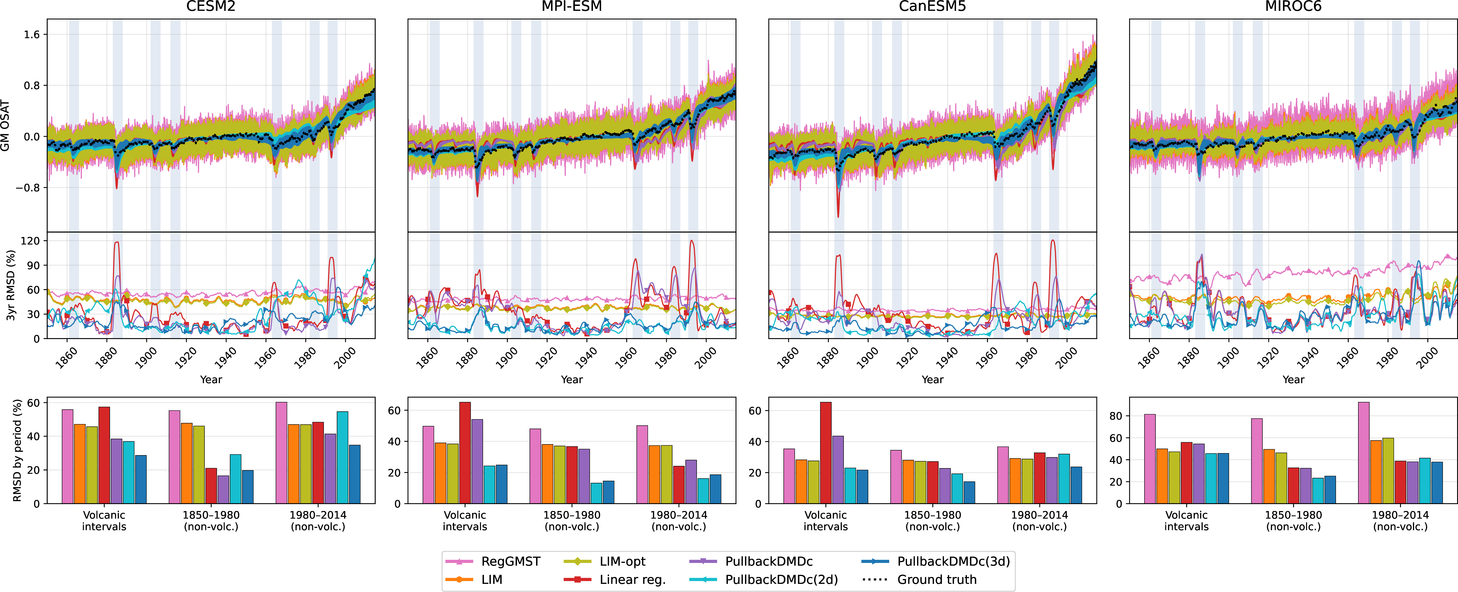
One can also notice that the overall correlation scores of the methods differ across ESMs; for example, the highest OSAT correlation score, up to \(0.9\), is achieved for CanESM5, which has the highest sensitivity to forcing and thus the strongest warming trend (cf. Fig. 2). This can be explained by the different signal-to-noise ratios of the forced component across ESMs, leading to higher average skill in more sensitive models. A similar dependence of signal-to-noise components on ESM sensitivity has been documented in previous studies of CMIP5 and CMIP6 models [20].
The next important conclusion we draw from the distributions is that all baseline methods except LR exhibit substantially higher uncertainty than PullbackDMDc, again reflecting their lack of strong external predictors of the forced response. As a result, they produce very noisy estimates with a much larger spread (cf. Fig. 2). The performance of these methods is sometimes much worse for SAT and SLP variables (cf. Fig. S6-S7). In SLP, the forced-response contribution to the simple global mean index is much weaker than internal variability. In fact, it is close to zero, with both positive and negative trends observed across ESMs. In SAT, there is a strong contrast between ocean and land variance, and some signatures of non-stationary change of the annual cycle over land and high latitudes, which formally contribute to the anomalies (see Sec. 3.2 for further details). These factors likely pose challenges for the methods that do not account for explicit forcing information.
All the conclusions here also hold for shorter target time-interval estimates, except that the errors of all methods increase (cf. Fig. S3, S8). This is expected because the sample size (e.g., the number of time steps) is reduced by almost \(2.5\) times, leading to greater uncertainty. This can be seen as one of the drawbacks of the class of methods that use a single climate realization for making estimates.
3.1.0.3 Choice of forcing in PullbackDMDc
Not all PullbackDMDc variants perform equally. Specifically, PullbackDMDc is sensitive to input forcing information. First, in all examples, PullbackDMDc benefits from separating the volcanic contribution from other slow contributions (e.g., greenhouse gases). Increasing forcing dimensionality substantially reduces global mean root mean square deviation (RMSD) and raw predictive skill (cf. Figs. 2, 1). This improvement reflects the fact that volcanic and long-term forcing activate distinct response patterns with different timescales. By explicitly including volcanic forcing, PullbackDMDc(2D)/(3D) better capture cooling effects during eruptions and reconstructs the temporal response structure during both weak and strong warming trends (cf. rows 2–3 of Fig. 2).
Next, there is a slight difference in the optimal combinations of long-term forcing predictors depending on the target variable: PullbackDMDc(2D) performs best for SLP, while PullbackDMDc(3D) performs best for OSAT and SAT (cf. Figs. 1, 2, S1, S2, and S6-S7). This suggests that OSAT/SAT benefits from a more complete representation of aerosol and greenhouse-gas forcing, while additional forcing input slightly degrades SLP performance, possibly because the lower signal-to-noise ratio in atmospheric circulation fields increases susceptibility to overfitting.
The optimal forcing dimension varies little across ESMs, suggesting robustness to the choice of climate generator, though the uncertainty regions overlap more for the less sensitive models, such as MIROC6 and MPI-ESM. Because the ESM ensemble mean provides a per-model ground truth, this comparison doubles as a principled way to select forcing predictors for PullbackDMDc. Such a systematic investigation of the optimal forcing is left to future work, as this choice likely varies with the target variable and dataset parameters.
3.2 PullbackDMDc modes↩︎
Recall that PullbackDMDc provides a spatiotemporal decomposition of a climate data cube into a sum of components characterized by a spatial pattern (dynamic mode) and the associated forced and internal time series, obtained by projecting the data onto these patterns. The leading modes with the slowest decay times represent the dominant dynamics captured by DMDc from the data. They offer a new lens for asking not only which patterns a model represents, but how it distributes variability and forced response across time scales relative to other models and to the reanalysis. Let us now provide a detailed example of such an evaluation using OSAT, along with results from SAT and SLP decompositions.
3.2.0.1 Reanalysis data decomposition
In the previous section, we presented the best forced-response estimates for PullbackDMDc(3D) on OSAT (for PullbackDMDc(3D) on SAT see Fig. S15-16 and SAT and PullbackDMDc(2D) on SLP see Fig. S17-S18). Therefore, we use this combination to decompose and interpret reanalysis data.
We now consider the top four dynamic modes of OSAT reanalysis (Fig. 3). The leading mode exhibits a global spatial pattern resembling the Atlantic Multidecadal Oscillation (AMO) [63], [64], with positive loadings concentrated in the mid- and North Atlantic and a secondary positive signature over the western Pacific. Its internal time series component is dominated by multidecadal variability, with a negative phase spanning roughly \(1900\)-\(1925\) followed by a positive phase from \(1930\)-\(1960\) (cf. smoothed dashed curve, Fig. 3); the corresponding autocorrelation function crosses zero near a \(20\)-year lag, consistent with a quarter-period of the underlying multidecadal oscillation, and exhibits secondary plateaus in the ENSO and PDO bands.

The second mode shows a complementary structure: a tripole pattern concentrated in the Pacific with comparatively weak Atlantic loadings, paired with an internal time series of similar multidecadal characteristics and autocorrelation shape to the first mode, together resembling a two-dimensional multidecadal oscillatory pair. The forced global warming response projects predominantly onto these first two modes, reflected in the large variance of the forced component of their respective time series relative to the remaining modes (orange time series), indicating that these large-scale, slowly-decaying dynamic modes are the most responsive to the forcing in the DMDc model inferred from data.
The complex-conjugate pair of modes with the third-longest decay time (modes \(3\) and \(4\) in Fig. 3) exhibits a two-dimensional ENSO/PDO-like spatial structure, with pronounced loadings over the tropical central and eastern Pacific. This is confirmed by the internal-component time series, which are characterized by comparatively fast autocorrelation decay and peaks within the characteristic ENSO and PDO temporal bands, consistent with their established interannual-to-decadal time scales. The dominant two-dimensional ENSO structure is well known and documented in observations [32], [65], [66], while the fact that this mode pair is complex conjugate is consistent with the conceptual recharge oscillator ENSO model [67]–[69]. The next modes (not shown) have less interpretable structure and contain more mixed time scales, ultimately resulting in noisy signals (cf. Fig. S9).
3.2.0.2 ESM data decomposition
Applying the same decomposition to the ESMs exposes systematic structural differences from the reanalysis. As a representative example, we introduce this decomposition for a single ensemble member of MPI-ESM (Fig. 4). In doing so, and comparing additional members from other ESMs (Fig. S10-S12), we highlight several differences of OSAT variability between ESMs and reanalysis (20CRv3).
First, PullbackDMDc(3D) does not place multidecadal variability in the leading mode. Instead, the leading mode is complex, forming a complex conjugate pair with the \(2\)nd mode. This conjugate pair of modes corresponds to ENSO-like variability in the representative MPI-ESM ensemble member. The strong multidecadal timescale observed in the reanalysis does not appear in either the \(3\)rd or \(4\)th modes. Upon further examination, we find neither an AMO-like spatial pattern nor pronounced multidecadal oscillations in the smoothed internal variability time series (cf. Fig. 4).
Second, the ENSO autocorrelation function looks more periodic than in reanalysis, suggesting more regular dynamics. This is complemented by the fact that modes \(3\)-\(4\) exhibit mostly decadal periodicity and are closer to the PDO, so the PDO appears more separated from ENSO in this realization than in observations. Even more regular ENSO-mode behavior is observed in CESM2 realizations (cf. Fig. S10).
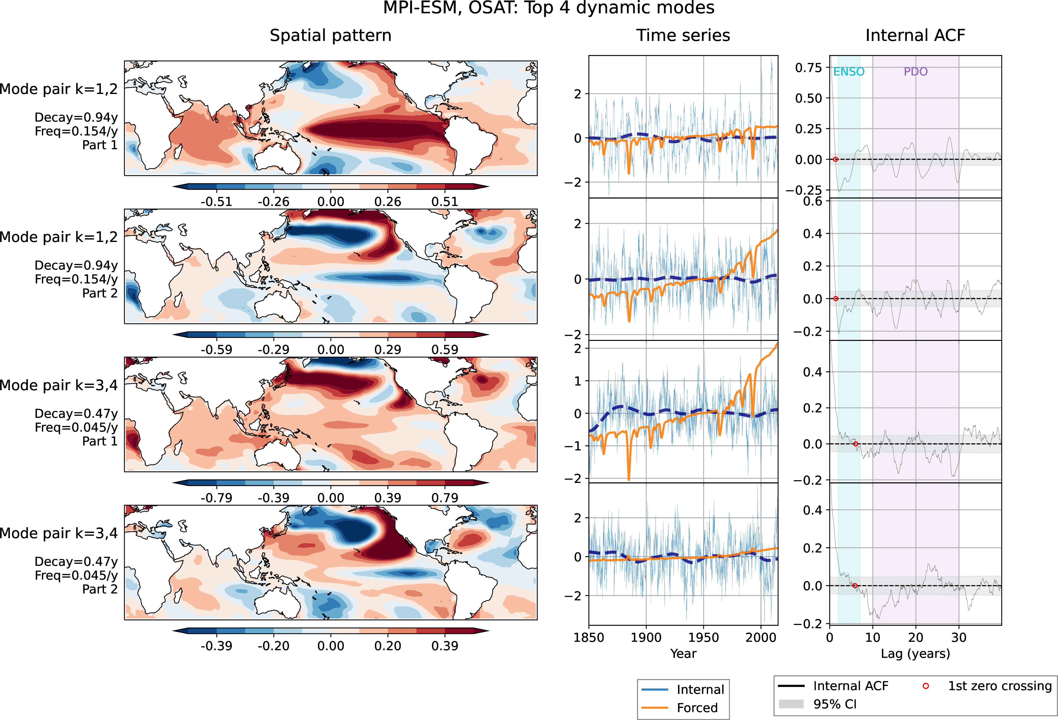
Third, in MPI-ESM, the forced response is not isolated as a distinct slow mode but is instead embedded within the faster ENSO- and PDO-related dynamics. Consequently, the forced component is reconstructed as a response to these faster modes, in contrast to the reanalysis case, where independent slow multidecadal modes carry most of the forced response.
3.2.0.3 Robustness across ESMs
To test whether the single-member contrasts above hold in general, we repeat the decomposition for every ensemble member of every ESM, zooming in on the dominant timescale of each internal component time series across all ensemble members and ESMs, estimated from its autocorrelation function by multiplying its zero-crossing time by \(4\) (Row 1 of Fig. 5). Note that this only represents the dominant time scale, meaning that the secondary timescales, such as the PDO in modes \(3\) and \(4\) of the reanalysis (cf. \(3\)rd column of Fig. 3), are missed. Modes \(1\) and \(2\) of all ESMs predominantly capture ENSO-scale variability (\(2\)-\(7\) years), with distributions tightly clustered around this range. Only a small number of outliers, primarily in CanESM5 and CESM2, exhibit longer timescales, likely reflecting a swap with the other modes in these members. Within the ENSO band, CESM2 shows slightly shorter periods (\(4\)-\(5\) years) compared to other models (\(5\)-\(7\) years).

Modes \(3\) and \(4\) of ESMs exhibit substantially broader distributions, including the PDO time interval, spanning approximately \(10\)-\(100\) years across models and ensemble members. While several members in each ESM reproduce multidecadal timescales comparable to the leading reanalysis modes, these occurrences are intermittent and co-exist with many realizations dominated by shorter variability. Specifically, reanalysis data have multidecadal timescales of \(80\) and \(60\) years in the first two modes. ESMs have dramatically fewer modes exceeding these timescale thresholds. This is clear in modes \(1\), \(2\), and \(4\). Looking more closely at mode \(3\), we find that the proportion of ensemble members with a mode \(3\) timescale greater than the reanalysis multidecadal timescale of \(60\) years ranges from \(\sim2-28\%\) across ESMs, and only \(\sim2-9.2\%\) for timescales greater than \(80\) years. This suggests that the ESMs mostly miss the observed multidecadal timescale. Other studies analyze similar discrepancies and confirm that there is a global multidecadal variability that ESMs underestimate, mostly in magnitude [64], [70]. A comprehensive study is presented in [71], where low-dimensional spatial and temporal features of this variability were identified in the ESMs. Remarkably, the most distinct component of it is AMO-like, strikingly similar to the pattern in the main mode of PullbackDMDc(3D) run on the reanalysis data.
To complement the analysis of multidecadal variability, we turn our attention to the total variance of the smoothed internal variability components (row \(2\) of Fig. 5). We clearly extract the high variance of modes \(1\) and \(2\) from the reanalysis and find only \(6\) ensemble members across all ESMs (excluding MIROC6) that have higher variance than the reanalysis. This indicates that the majority of the dominant timescales of the internal variability time series that exceed the reanalysis timescale have weak amplitudes and/or low-variance spatial patterns, aligning with previous studies [64], [70], [71].
We now examine the relative contribution of the forced response extracted by PullbackDMDc(3D), quantified as the ratio of the variance of the forced component to that of the full time series, and assess whether the finding from the single MPI-ESM member generalizes across ESMs (Row \(3\) of Fig. 5). In reanalysis, the forced variance fraction is large in modes \(1\) and \(2\), consistent with the forced global warming response projecting predominantly onto the leading slow multidecadal modes. In contrast, the forced response in ESMs tends to project more strongly onto modes \(3\) and \(4\), which carry slower decadal-to-multidecadal time scales than the leading ENSO-like modes. Among modes \(1\) and \(2\), CanESM5 and MPI-ESM show comparatively larger forced contributions, while CESM2 (excluding ensemble members with apparent mode swaps) and MIROC6 show smaller ones. Overall, the forced variance fraction is more distributed across all four modes, reflecting the absence of a dominant slow multidecadal mode that would otherwise capture most of the forced signal. Across all modes, the forced variance fractions are largest for CanESM5, consistent with its strong sensitivity to external forcing relative to the other tested ESMs, also documented in Sec. 3.1.
Taken together, these robustness diagnostics paint a consistent and physically interpretable picture: reanalysis is dominated by slow multidecadal modes that capture both the dominant internal variability and most of the forced signal, while ESMs systematically underrepresent this slow multidecadal structure, distributing the forced response across faster ENSO- and PDO-like dynamics instead. This structural difference between reanalysis and ESMs, robust across ensemble members, suggests that PullbackDMDc provides a useful diagnostic framework for evaluating how well ESMs reproduce the dominant modes of climate variability and their response to external forcing.
3.2.0.4 SAT/SLP: the seasonal cycle trend
The same analysis can be carried out for the PullbackDMDcdecomposition of other variables. For SAT, the optimal variant was PullbackDMDc(3D), while for SLP it was PullbackDMDc(2D). Here, we highlight one result that does not appear in the OSAT decomposition.

We turn our focus to the dominant time scales extracted from the autocorrelation functions of internal-mode time series for SAT and SLP, for modes \(1\)-\(4\) (Fig. 6). For SAT, the first two modes capture the ENSO and multidecadal time scales we observed earlier in OSAT. However, modes \(3\)-\(4\) exhibit a strong annual autocorrelation, which was not observed in OSAT. An annual period is not, at first sight, expected in anomalies: the standard anomaly computation removes only the mean seasonal cycle, and any slow, non-stationary change in the seasonal cycle’s shape is not captured by this procedure, so its deviation from the long-term average shape remains in the anomalies and retains an annual period. This non-stationarity is observed in the reanalysis over land and high latitudes, which were largely excluded in the OSAT case (cf. spatial patterns in Fig. S12). Instead, the dominant timescales for modes \(1\)-\(4\) across all ESMs span both ENSO and PDO timescales, with mode \(2\) spanning longer time scales in CanESM5 and MPI-ESM, while the annual period does not appear in these modes (cf. Fig. 6 and Fig. S17-S18). In other words, the ESMs tend to underrepresent the non-stationary change of the seasonal cycle that the reanalysis clearly retains.
A similar picture is found in SLP, where we find that modes \(3\) and \(4\) of the reanalysis again exhibit a non-stationary seasonal cycle with a strong annual period (cf. bottom row of Fig. 6). . In ESMs, however, some realizations do exhibit near-annual time scales in the same modes, but the period is not strongly annual, and the autocorrelation decays much faster, quickly approaching the confidence levels (cf. Figs. S13-S14), suggesting that the non-stationary seasonal cycle is considerably weaker in ESMs than in reanalysis. These findings together suggest that ESMs tend to underrepresent the non-stationary change of the seasonal cycle in both SAT and SLP, though the degree of underrepresentation differs between variables.
3.2.0.5 DMD eigenvalues
Another diagnostic for the time scales of modes extracted by PullbackDMDc(3D) are the DMD eigenvalues (Fig. 7 and Fig. S4). The ordering of the leading oscillatory eigenmodes differs substantially between datasets. This difference between reanalysis and ESMs lies in how they rank purely real, non-oscillatory modes versus oscillatory modes by their decay timescales (\(| \lambda |\)). In reanalysis, the rank-1/2 modes are purely real and thus do not oscillate, followed by the pair of conjugate rank-3/4 oscillatory modes. In contrast, this pattern is reversed in ESMs: the rank-1/2 eigenvalues are almost always complex conjugates and thus oscillatory, with purely real modes often occurring at rank-3/4.
We emphasize that DMD eigenvalue time scales are not in one-to-one correspondence with dominant time scales inferred from autocorrelation functions. The former reflect the exponential decay rates of optimally fitted linear modes, while the latter capture the peak or characteristic decorrelation behavior of a generally non-Markovian, multi-timescale process projected onto dynamic modes. In particular, for oscillatory and long-memory variability, these two notions of “time scale” may differ substantially, yet empirically, our results show they generally remain consistent in separating fast (ENSO-like) from slow (multidecadal) variability.

From this perspective, the key result is that ESMs and reanalysis disagree on which timescale of variability is more persistent. ESMs assign greater persistence to ENSO/PDO-scale modes, whereas reanalysis assigns greater persistence to multidecadal modes - a reversal that holds even though both reproduce variability at both timescales.
4 Discussion and Conclusion↩︎
In this work, we proposed PullbackDMDc, which combines LIM-based dynamical structure with explicit external forcing in the form of a non-stationary linear stochastic dynamical system. Our method uses pullback attractor estimation to formally separate forced-response and internal-variability contributions and to provide a decomposition of a single spatiotemporal climate signal into a collection of spatial patterns, each accompanied by a forced and an internal time series.
To assess the method’s performance, we evaluated forced-response estimation skill against several baselines using ground truth from large ESM ensembles. PullbackDMDc consistently matches or exceeds the skill of linear regression across temperature and pressure variables, while outperforming methods that do not incorporate forcing information. A key practical finding is that performance depends on the choice of forcing predictors: richer forcing representations improve temperature skill but can degrade pressure skill, and ESM ground truth provides a natural framework for identifying optimal combinations of predictors.
The spatiotemporal decomposition reveals a physically interpretable picture of how ESMs differ from reanalysis. In reanalysis, the leading modes capture slow AMO-like multidecadal variability, and the forced response projects predominantly onto these slow structures. ESMs systematically prioritize faster ENSO-scale dynamics in the leading modes, underrepresent multidecadal variability, and distribute the forced response across a broader set of modes. This structural difference likely reflects the well-reported underestimation of the amplitude of multidecadal variability in current ESMs [64], [70], [71]. Additionally, reanalysis retains signatures of a non-stationary seasonal cycle that ESMs largely fail to reproduce, suggesting further avenues for model evaluation using the PullbackDMDc.
The ensemble-mean forced response as a ground truth estimator is known to be inaccurate for small ensembles or under large internal variability [44]; more advanced estimators such as signal-to-noise maximizing patterns, extended EOFs, or ensemble-based linear dynamical modes [43]–[45], [72] could provide more reliable benchmarks and would be worth exploring in future evaluations. Here, we mitigated this issue by using large ensembles of \(40+\) members and applying a simple smoothed ensemble mean to SLP, which substantially reduces ground-truth uncertainty [45]. Similarly, our baseline comparison is intentionally focused on a small set of simple methods and four ESMs; a broader comparison with state-of-the-art methods across more models would be valuable. To this end, PullbackDMDc has been submitted to Tiers \(2\) and \(3\) of ForceSMIP [21], where a systematic comparison with the broader community of methods is expected when results are released.
As a decomposition method, PullbackDMDc shares conceptual ground with several existing approaches that target time scale separation. For example, average predictability time decomposition [73], [74] relies on a dynamical system model and identifies patterns that maximize predictability time; low-frequency component analysis [31] identifies patterns that emphasize slower time scales via fingerprinting. LDM method [39], [75], introduced earlier, trains latent time series of the modes, thereby enabling more effective noise filtering; a similar idea is used in optimized DMD [76], [77], which suggests a natural further extension of PullbackDMDc to improve the projected forced-response time series. A systematic extension and comparison of these and other decomposition approaches would be a valuable step toward a unified framework for separating forced and internal variability.
Finally, we highlight three methodological directions we consider most promising for overcoming inherent limitations of the PullbackDMDc framework. First, the framework is linear, meaning that the pullback attractor is represented as a single trajectory and the decomposition into forced and internal components is exact only under linear dynamics. In nonlinear systems, this structure would generally become set-valued, and a clean forced–internal separation is not guaranteed, requiring new formal definitions of forced response beyond the current framework. The nonlinear parameterizations, such as polynomials [78]–[80], low-dimensional neural networks [36], [81] and Koopman operators in latent state space [82]–[84], given the forcing predictors at the input, fall naturally into the same non-autonomous dynamical system framework, representing the most straightforward generalization. Beyond these, kernel-based methods [85], neural operators [86], or manifold learning approaches [87] could further capture state-dependent variability and regime behavior that lie outside the linear framework.
Second, the estimation of the dynamical operator \(\boldsymbol{A}\) from finite, noisy data is a primary source of uncertainty. In practice, decay times should be interpreted as lower bounds on physically relevant timescales under the current estimator. Noise and finite-sample-length bias bias estimates toward faster decorrelation and may obscure weak but persistent multidecadal structure. This effect is particularly relevant given that a \(\approx100\)-year forcing history may be insufficient for full convergence of the pullback dynamics when intrinsic timescales are longer than those recovered here. Thus, improving estimation of \(\boldsymbol{A}\) is a priority for future work. Noise-aware filtering strategies, latent dynamical system approaches mentioned above, regularization, and physically informed constraints on the operator spectrum may shift estimated decay times toward longer values and improve recovery of weak multidecadal signals that are currently suppressed by sampling noise.
Third, methodological choices such as time lag, truncation level, and forcing specification influence results. While sensitivity tests indicate qualitative robustness, these parameters may contribute to mode mixing, particularly in separating oscillatory and non-oscillatory structures. Furthermore, such parameters jointly determine the effective spectral content of the learned operator and may explain part of the observed reversal of mode ordering between reanalysis and ESMs. In particular, lag-dependent spectral mixing combined with noise and finite-sample effects may bias leading modes toward faster oscillatory variability in ESMs, even when slower modes are present but weak. Therefore, a systematic exploration of this parameter space is warranted to reduce estimation bias and improve the recovery of long-timescale variability.
Implementing any of these extensions will require careful attention to interpretability, which remains central to the climatological utility of the PullbackDMDc framework. More broadly, PullbackDMDc illustrates how classical non-autonomous dynamical-systems theory and modern data-driven decomposition can be brought together to read a single climate record as the fading imprint of its own forcing history. We expect our approach to extend naturally to other variables, to coupled multivariate fields, and, eventually, to the nonlinear regimes.
This work was supported by the European Research Council (ERC) under the ERC Synergy Grant “Understanding and Modeling the Earth System with Machine Learning” (USMILE; grant agreement 855187), by the European Union’s Horizon Europe research and innovation programme under projects “European Lighthouse of AI for Sustainability” (ELIAS; 101120237) and “Artificial Intelligence and Machine Learning for Enhanced Representation of Processes and Extremes in Earth System Models” (AI4PEX; 101137682), and by the Generalitat Valenciana, through the PROMETEO project “AI4CS: Artificial Intelligence for complex systems” (CIPROM/2021/056, 2021–2025).
The main code base for this project can be found here https://github.com/IPL-UV/PullbackDMDc.
The reanalysis data from observations can be accessed from https://www.psl.noaa.gov/thredds/catalog/Datasets/20thC_ReanV3/Monthlies/2mSI-MO/catalog.html on https://www.psl.noaa.gov/data/gridded/data.20thC_ReanV3.html.
The ESM data can be accessed from here https://gdex.ucar.edu/datasets/d651039/.
The radiative forcing information is from the IPCC AR6 Chapter 7 ([56]; accessible https://raw.githubusercontent.com/IPCC-WG1/Chapter-7/main/data_output/AR6_ERF_1750-2019.csv) and interpolated to a monthly resolution.
The code for running the baseline methods: RegGMST, LIM, and LIM-opt was adapted from https://github.com/karenamckinnon/forcesmip associated with the ForceSMIP project.
4.1 Linear inverse models (LIM)↩︎
In LIM, we assume the time series of principal components comes from the low-dimensional stochastic dynamical system \[\frac{d \boldsymbol{x}(t)}{dt} = \boldsymbol{L}\boldsymbol{x}(t) + \boldsymbol{\eta}(t).\] The solution to this system for the discrete time lag \(\tau=1\) is: \[\boldsymbol{x}(t) = e^{L } \boldsymbol{x}(t-1) + \int_{t-1}^{t} e^{\boldsymbol{L} (t - s)} \eta(s)\, ds.\] Using \(\boldsymbol{A}=e^{\boldsymbol{L} }\) and \(\boldsymbol{\xi}(t)=\int_{t-1}^{t} e^{\boldsymbol{L} (t - s)} \eta(s)\, ds\), we write discrete LIM with a random component as \[\boldsymbol{x}(t) = \boldsymbol{A} \boldsymbol{x}(t-1) + \boldsymbol{\xi}(t).\] In LIM, we estimate \(\boldsymbol{A}\) via the least squares problem \[\label{iouvfbkl} \min_{\boldsymbol{A}} \sum_t\| \boldsymbol{x}(t) - \boldsymbol{A}\boldsymbol{x}(t-1)\|_2^2.\tag{14}\] Dynamic mode decomposition (DMD) [48] is the deterministic component of a discrete-time LIM that includes an eigendecomposition of \(\boldsymbol{A} \boldsymbol{W} = \boldsymbol{\Lambda} \boldsymbol{W}\). See Section c for the details of DMD.
Replicating [16], we use the eigendecomposition of \(\boldsymbol{A}\) to estimate the forced response with LIM. Specifically, we use the least damped mode, \(\boldsymbol{w}_{1}\), the eigenvector of \(\boldsymbol{A}\) associated with the eigenvalue with the largest absolute value. This mode is almost always real-valued; thus, we continue with this assumption. When mapped back into the observed space using the EOF matrix \(\boldsymbol{U}\), we obtain the spatial pattern that decays slowest in time, \(\boldsymbol{U}\boldsymbol{w}_{1}\). We denote the timeseries associated with this mode as \(z_1(t)\), namely the first entry of \(\boldsymbol{z}(t)\) that solves \(\boldsymbol{W}\boldsymbol{z}(t) = \boldsymbol{x}(t)\). Using these quantities, we construct the forced response as \[\label{eq:32lim95forced95response} \tilde{\boldsymbol{x}}^{(f)}(t) \approx \boldsymbol{U}\boldsymbol{w}_1 z_{1}(t).\tag{15}\] LIM was an early, primitive dynamical-system-based forced-response estimator. LIM forced response estimates do not incorporate forcing as input and are often noisy.
4.2 LIM with Optimal Perturbation Patterns (LIMopt)↩︎
To combat noisy forced response estimates, LIM with optimal perturbation patterns (LIMopt) provides a smoother estimate of the forced response by evolving the patterns in \(\boldsymbol{A}\) over an optimal perturbation time [16], [43], [50]. LIMopt uses the LIM dynamical system model and its discrete-time realization. Thus, \(\boldsymbol{A}\) is estimated using the least-squares solution to 2 .
The smoothing of LIMopt comes in the optimal perturbation filter. Specifically, we compute the approximate time evolution matrix of the PCs over \(\tau_e\) time steps as \(\boldsymbol{A}^{\tau_e}\). Now we compute the Singular Value Decomposition (SVD) \(\boldsymbol{A}^{\tau_e} = \boldsymbol{\Psi} \boldsymbol{\Sigma} \boldsymbol{\Phi}^\top\).
LIMopt uses the patterns in the left and right singular vectors associated with the largest singular values of \(\boldsymbol{A}^{\tau_e}\) to estimate the forced response as \[\label{eq:32limopt95forced95response} \tilde{\boldsymbol{x}}^{(f)}(t) \approx \boldsymbol{U}\boldsymbol{\psi}_1 \boldsymbol{\phi}_1^\top \boldsymbol{x}(t).\tag{16}\] Notice \(\boldsymbol{\psi}_1 \boldsymbol{\phi}_1^\top\) is a rank-\(1\) approximation of \(\frac{1}{\lambda_1}\tilde{\boldsymbol{A}}\). This method can be separated into a forcing pattern, defined by \(\boldsymbol{U}\boldsymbol{\psi}_1\) and its contribution over time \(\boldsymbol{\phi}_1^T \boldsymbol{x}(t)\).
The intuition is that the forcing pattern is more distinct over the amplitude over the time evolution \(\tau_e\). The spatial pattern of forcing is \(\boldsymbol{\psi}_1\) re-scaled out of the PC domain using the EOFs in \(\boldsymbol{U}\). The scale of this pattern at time \(t\) is \(\boldsymbol{\phi}_1^T \boldsymbol{x}(t)\). So we are evolving \(\tilde{\boldsymbol{x}}(t)\) over \(\tau_e\) time steps using \(\boldsymbol{A}^{\tau_e}\) and scaling by \(\frac{1}{\lambda_1}\), then computing the optimal time contribution of the fixed forced response pattern using this evolved signal.
4.3 Dynamic Mode Decomposition↩︎
Dynamic Mode Decomposition (DMD) [48] is essentially the LIM model without the stochastic component [88] and approximates the Koopman mode decomposition [89]. The machinery of DMD computes the eigendecomposition of \(\boldsymbol{A}\), then uses it to construct a reduced-order model. In early works, DMD was formulated as a method that encapsulates both computing the PC time series of the data and estimating the eigendecomposition of \(\boldsymbol{A}\) in a single step. There are many more DMD variants than LIM variants, including more robust variants, and the incorporation of control (to be discussed later) [89].
In classic DMD language, the dynamic modes are the eigenvectors of \(\boldsymbol{A}\) in the original space (before EOF analysis): the columns \(\boldsymbol{\phi}_r\) of \(\boldsymbol{\Phi} = \boldsymbol{U}\boldsymbol{w}_r\). The scale (a.k.a. amplitude) of these dynamic modes solves are the entries \(b_r\) of the \(\boldsymbol{b}\) that solves \(\boldsymbol{\Phi} \boldsymbol{b} = \boldsymbol{x}(0)\). \(\lambda_r = e^{\tau \omega_r}\) is the \(r\)th discrete eigenvalue associated with this mode and represents its temporal evolution over the time lag \(\tau\). The continuous-time eigenvalue is \(\omega_r\). The DMD-reconstruction of \(\boldsymbol{x}(t)\) [89] is \[\label{eq:32dmd} \boldsymbol{x}(t) \approx \sum_r \boldsymbol{\varphi}_r e^{t \omega_r} b_r.\tag{17}\] Using this, we can decompose our data into spatial patterns \(\boldsymbol{\varphi}_r\) and associated time series \(\exp(t \omega_r) b_r\). Note that this is essentially a prediction of the initial amplitudes of the modes by a linear DMD model. Therefore, it works under the strong assumption that the data source is a linear, low-dimensional deterministic system. If this is not the case, this prediction brings an error growing with time \(t\).
4.4 Dynamic Mode Decomposition with Control↩︎
Dynamic Mode Decomposition with Control (DMDc) [42] assumes the discrete-time linear dynamical system with control \[\label{eq:32discrete32time32forced} \boldsymbol{x}(t) = \boldsymbol{A} \boldsymbol{x}(t-1) + \boldsymbol{B} \boldsymbol{y}(t-1).\tag{18}\] This method improves upon the forced-response models in LIM-variant baselines by including forcing in the control term \(\boldsymbol{y}(t)\). It improves over the linear regression baselines because it includes the dynamical component from LIM.
In our work, we replace \(\boldsymbol{y}(t-1)\) with \(\boldsymbol{y}(t)\) to align with the convention commonly adopted in the climate literature. Mathematically, this change reflects only a difference in indexing and does not alter the underlying dynamics. More importantly, if we go from a continuous formulation, the forcing term at time \(t\) is dynamically integrated over the interval between the previous observed state (at \(t-1\)) and the moment \(t\). Given that it’s slow, \(\boldsymbol{y}(t)\) is close to \(\boldsymbol{y}(t-1)\), and one can show that the first-order approximation of the integral would be a linear function of \(\boldsymbol{y}(t)\). Therefore, in the main text, we treat \(\boldsymbol{y}(t)\) as the forcing actually observed at the month \(t\).
The initial formalization of DMDc is performed on the raw data rather than on the PC time series. We choose to run PCA, then fit a full-rank DMDc model for computational efficiency and to enable a simpler comparison with LIM forced-response models. Thus, in the DMDc model, finding \(\boldsymbol{A}\) and \(\boldsymbol{B}\) is reduced to a simple least-squares linear regression problem \[\begin{align} &\min_{\boldsymbol{A},\boldsymbol{B}} \sum_t \|\boldsymbol{x}(t) - \boldsymbol{A} \boldsymbol{x}(t-1) - \boldsymbol{B} \boldsymbol{y}(t-1) \|_2^2. \end{align}\]
Once again, we can use the eigenvalue decomposition \(\boldsymbol{A}\boldsymbol{W} = \boldsymbol{W} \boldsymbol{\Lambda}\). Since this eigenvalue decomposition mirrors what is done in LIM and DMD, it is standard to use the same standard model and eigenvalue analysis to understand the evolution of the climate variable in the absence of the forcing signal \(\boldsymbol{y}(t)\) [41].
4.5 Rotation of complex-conjugate mode pairs↩︎
Here we describe the rotation procedure applied to each complex-conjugate pair of dynamic modes and their associated forced and internal time series to improve the physical interpretability of the decomposition by PullbackDMDc.
We first verify that the projected internal time series \(z_\ell^{(i)}(t)\) form complex-conjugate pairs. Since \(\boldsymbol{x}^{(i)}(t)\) is real and \(\boldsymbol{z}^{(i)}(t) = \boldsymbol{W}^{-1}\boldsymbol{x}^{(i)}(t)\), and the rows of \(\boldsymbol{W}^{-1}\) corresponding to a conjugate eigenvector pair are themselves conjugate, we have \(z_{\ell+1}^{(i)}(t) = \overline{z_\ell^{(i)}(t)}\), and analogously \(z_{\ell+1}^{(f)}(t) = \overline{z_\ell^{(f)}(t)}\).
The internal contribution of the conjugate pair \((\boldsymbol{w}_\ell, \overline{\boldsymbol{w}_\ell} = \boldsymbol{w}_{\ell+1})\) to \(\boldsymbol{x}^{(i)}(t)\) is the sum of two conjugate terms, which is purely real: \[\begin{align} \begin{aligned} \boldsymbol{w}_\ell z_\ell^{(i)}(t) + \overline{\boldsymbol{w}}_\ell \overline{z_\ell^{(i)}(t)} = &2\mathrm{Re}\left(\boldsymbol{w}_\ell z_\ell^{(i)}(t)\right) \\ = &2\mathrm{Re}(\boldsymbol{w}_\ell)\mathrm{Re}\left(z_\ell^{(i)}(t)\right) \\ &- 2\mathrm{Im}(\boldsymbol{w}_\ell)\mathrm{Im}\left(z_\ell^{(i)}(t)\right). \end{aligned} \end{align}\] This can be written as a product of two \(2\)D real matrices by stacking the real and imaginary parts of the mode and its internal time series: \[\begin{align} \widetilde{\boldsymbol{W}}_\ell &= [2\mathrm{Re}(\boldsymbol{w}_\ell),\, -2\mathrm{Im}(\boldsymbol{w}_\ell)]\in \mathbb{R}^{K\times 2},\\ \widetilde{\boldsymbol{Z}}^{(i)}_\ell &= \left[\mathrm{Re}\left(\boldsymbol{z}_\ell^{(i)}\right),\, \mathrm{Im}\left(\boldsymbol{z}_\ell^{(i)}\right)\right] \in \mathbb{R}^{T\times 2}, \end{align}\] so that the contribution equals \(\widetilde{\boldsymbol{W}}_\ell \left(\widetilde{\boldsymbol{Z}}^{(i)}_\ell\right)^\top\).
The \(2\)D PCA rotation is computed via QR decompositions \(\widetilde{\boldsymbol{W}}_\ell = \boldsymbol{Q}_W \boldsymbol{R}_W\) and \(\widetilde{\boldsymbol{Z}}^{(i)}_\ell = \boldsymbol{Q}_Z \boldsymbol{R}_Z\), followed by the SVD \(\boldsymbol{R}_W \boldsymbol{R}_Z^\top = \boldsymbol{U} \boldsymbol{\Sigma} \boldsymbol{V}^\top\). Note that \(\boldsymbol{R}_W \in \mathbb{R}^{2\times 2}\) is invertible because \(\widetilde{\boldsymbol{W}}_\ell\) has full column rank: its two columns \(2\mathrm{Re}(\boldsymbol{w}_\ell)\) and \(-2\mathrm{Im}(\boldsymbol{w}_\ell)\) are linearly independent whenever \(\boldsymbol{w}_\ell\) is not purely real, which holds for any genuinely oscillatory complex-conjugate pair. The left singular vectors of \(\widetilde{\boldsymbol{W}}_\ell(\widetilde{\boldsymbol{Z}}^{(i)}_\ell)^\top\) are exactly \(\boldsymbol{Q}_W \boldsymbol{U}\), which is orthogonal since it is a product of two orthogonal matrices. This defines a \(2\times 2\) invertible linear map \(\boldsymbol{P} = \boldsymbol{R}_W^{-1}\boldsymbol{U} \in \mathbb{R}^{2\times 2}\) acting on \(\widetilde{\boldsymbol{W}}_\ell\) from the right, yielding the rotated patterns and time series: \[\begin{align} [\widehat{\boldsymbol{w}}_\ell,\, \widehat{\boldsymbol{w}}_{\ell+1}] &= \boldsymbol{Q}_W \boldsymbol{U} = \widetilde{\boldsymbol{W}}_\ell \boldsymbol{P} \in \mathbb{R}^{K\times 2},\\ [\widehat{z}^{(i)}_\ell,\, \widehat{z}^{(i)}_{\ell+1}] &= \widetilde{\boldsymbol{Z}}^{(i)}_\ell \boldsymbol{P}^{-\top} \in \mathbb{R}^{T\times 2}, \end{align}\] where \(\boldsymbol{P}^{-\top} = \boldsymbol{R}_W^\top \boldsymbol{U}\) follows from \(\boldsymbol{P}^{-1} = \boldsymbol{U}^\top \boldsymbol{R}_W\). Of course, this rotation preserves the reconstruction of the internal component: \[\begin{align} (\widetilde{\boldsymbol{W}}_\ell \boldsymbol{P}) (\widetilde{\boldsymbol{Z}}^{(i)}_\ell \boldsymbol{P}^{-\top})^\top &= \widetilde{\boldsymbol{W}}_\ell \boldsymbol{P} \boldsymbol{P}^{-1} (\widetilde{\boldsymbol{Z}}^{(i)}_\ell)^\top = \widetilde{\boldsymbol{W}}_\ell(\widetilde{\boldsymbol{Z}}^{(i)}_\ell)^\top. \end{align}\]
4.6 Data matrix construction and lag notation↩︎
For simplicity of exposition in the main text, we presented the method assuming the sampling step of the data coincides with the lag step of the trained model, i.e., a model of the form \[\label{eq:32supp95linear95system} \boldsymbol{x}(t) = \boldsymbol{A}\boldsymbol{x}(t-1) + \boldsymbol{B}\boldsymbol{y}(t) + \boldsymbol{\xi}(t),\tag{19}\] where “\(t-1\)” denotes one native sampling step (in our case, months). In practice, however, the model is trained at a chosen lag \(\tau\) (3 months in the main text), which need not equal the native sampling interval of the underlying anomaly fields. The model fit is therefore \[\label{eq:32supp95linear95system95tau} \boldsymbol{x}(t) = \boldsymbol{A}\boldsymbol{x}(t-\tau) + \boldsymbol{B}\boldsymbol{y}(t) + \boldsymbol{\xi}(t),\tag{20}\] with \(\boldsymbol{A}\) a \(\tau\)-step propagator rather than a \(1\)-native-step propagator.
To fit Eq. 20 , we retain all snapshots at native (monthly) resolution, \(\boldsymbol{X} = [\boldsymbol{x}(1), \boldsymbol{x}(2), \dots, \boldsymbol{x}(T)]\), but construct the paired snapshot matrices by pairing each snapshot with the one \(\tau\) steps ahead, rather than one step ahead: \[\boldsymbol{X} = \big[\boldsymbol{x}(1), \boldsymbol{x}(2), \dots, \boldsymbol{x}(T-\tau)\big], \qquad \boldsymbol{X}' = \big[\boldsymbol{x}(1+\tau), \boldsymbol{x}(2+\tau), \dots, \boldsymbol{x}(T)\big].\] That is, column \(j\) of \(\boldsymbol{X}'\) is the snapshot occurring \(\tau\) steps after column \(j\) of \(\boldsymbol{X}\), while consecutive columns within each matrix remain separated by a single native step, not by \(\tau\). This design choice makes full use of all available native-resolution snapshots rather than subsampling every \(\tau\)-th one. We solve the DMDc regression \(\boldsymbol{X}' \approx \boldsymbol{A}\boldsymbol{X} + \boldsymbol{B}\boldsymbol{Y}\) for the propagator \(\boldsymbol{A}\) associated with lag \(\tau\).
The pullback-attractor solution of Eq. 20 retains the same functional form as in the unit-lag case, but with \(\tau\) appearing explicitly in the spacing of past terms under both sums: \[\begin{align} \begin{aligned}\label{eq:decompose95ds95tau} \boldsymbol{x}(t| \boldsymbol{x}_0,t_0) \underset{t_0 \to -\infty}{\xrightarrow{}} &\underbrace{\sum\limits_{j=0}^{\infty} \boldsymbol{A}^{j}\boldsymbol{B} \boldsymbol{y}(t-j\tau)}_{\text{forced response}} + \underbrace{\sum\limits_{j=0}^{\infty} \boldsymbol{A}^{j}\boldsymbol{\xi}(t-j\tau)}_{\text{internal variability}}\\ &= \boldsymbol{x}^{(f)}(t) +\boldsymbol{x}^{(i)}(t). \end{aligned} \end{align}\tag{21}\] In this case, each term in the forced-response and internal-variability sums is spaced \(\tau\) steps apart in the past, rather than one native step. In practice, this means the algorithm computes the forced response as a deterministic (noise-free) prediction, initialized from the first \(\tau\) points of the forcing history \(\boldsymbol{y}\), each propagated forward recursively via Eq. 20 , then stitched back together. For example, for \(\tau=3\), we have three matrices of forced response predictions \[\begin{align} \begin{aligned} \boldsymbol{X}_1^{(f)} &= \begin{bmatrix} \boldsymbol{x}(1)^{(f)} & \boldsymbol{x}(1+3)^{(f)} & \cdots & \boldsymbol{x}(T-2)^{(f)}\end{bmatrix},\\ \boldsymbol{X}_2^{(f)} &= \begin{bmatrix} \boldsymbol{x}(2)^{(f)} & \boldsymbol{x}(2+3)^{(f)} & \cdots & \boldsymbol{x}(T-1)^{(f)}\end{bmatrix},\\ \boldsymbol{X}_3^{(f)} &= \begin{bmatrix} \boldsymbol{x}(3)^{(f)} & \boldsymbol{x}(3+3)^{(f)} & \cdots & \boldsymbol{x}(T)^{(f)}\end{bmatrix}. \end{aligned} \end{align}\] When stitched together, one column at a time, they contain the entire forced response timeseries. This makes \(\tau\) an explicit hyperparameter of PullbackDMDc, which we tune empirically below, rather than a quantity fixed by the notation in Eq. 19 .
4.7 Parameters and Data Preprocessing↩︎
For each ESM ensemble member and observations, we compute anomalies, then run area-weighted Principal Component Analysis (PCA), a.k.a. Empirical Orthogonal Function (EOF) analysis. This common step allows us to avoid invertibility problems with the matrix \(\boldsymbol{W}\) in computing PullbackDMDc internal and forced timeseries. The resulting Principal Components (PCs) are then fed into our methods. We use EOFs (a.k.a. PC basis vectors) to reconstruct the original field for visualizing the spatial patterns of dynamic modes of variability. For SAT and OSAT, we use \(20\) PCs, following the approach used for similar forced-response estimation methods in ForceSMIP [21]. However, for SLP the forced response signal is much smaller than the variance of the residual fast internal variability and noise. As a result, a small number of leading PCs cannot adequately capture this weaker forced signal. To address this and ensure its representation, we retain \(200\) PCs for SLP.
4.7.0.1 Ground truth ensemble mean
Our ground-truth for the forced response is the ESM ensemble mean. This is computed for each ESM by averaging the anomalies over all ensemble members. The same factors that lead to selecting a larger number of PCs for SLP introduce additional error into the raw ensemble-mean forced-response estimates. Therefore, we smooth the ensemble-mean SLP anomalies using a \(3\)-year sliding window to improve the computed ground-truth forced-response signal for comparison.
4.7.0.2 Forcing
Our forcing signal for PullbackDMDc variants and Linear Regression is yearly forcing, interpolated to a monthly resolution, from the IPCC AR6 Chapter 7 [56]. We first test the total effective radiative forcing to align with what was used in various submissions to ForceSMIP [21]. This signal is essentially a one-dimensional compression of all forcing information. We call the PullbackDMDc variant that uses this forcing “PullbackDMDc.” This forcing is also used for Linear Regression.
We examine how the performance of PullbackDMDc varies with the provided forcing signal, specifically its dimension. Therefore, we test PullbackDMDc with two more variants of input forcing information with dimensions \(2\) and \(3\). As a \(2\)-dimensional set of forcings, we choose time series of two main contributors: CO\(_2\) emissions and volcanic activity. We call PullbackDMDc with these forcings “PullbackDMDc(2D).”
For our next, \(3\)-dimensional approximation of forcing information, we replace CO\(_2\) with greenhouse gas concentrations, keep volcanic activity, and add aerosols. The PullbackDMDc variant that uses these data is called “PullbackDMDc(3D).” The exploration of the forcing combinations can be extended, but here we restrict ourselves to these three cases to assess the basic effect.
Regardless of the forcing signal’s dimension, these data are mean-centered and scaled by their standard deviation over the target interval.3 The past forcing data used in PullbackDMDc variants is scaled by coefficients obtained on the same interval.
4.7.0.3 Time lags
For methods with a dynamical component (PullbackDMDc variants, LIM, LIMopt), we tested time lags of \(1\), \(3\), \(6\), and \(12\) years and found that a lag of \(3\) years generally produces the most accurate forced-response estimates across ESMs and climate variables. We therefore present results obtained with a \(3\)-year lag throughout this manuscript. In linear dynamical frameworks, the propagator matrix \(\boldsymbol{A}\) captures predictable large-scale variability, while rapidly decorrelating processes are treated as stochastic residuals [29]. Increasing the lag tends to reduce the representation of faster modes such as ENSO while emphasizing slower variability and the forced response. A \(3\)-year lag, therefore, provides a practical balance between retaining key internal variability and isolating slower, predictable dynamics. This choice is also consistent with previous LIM-based analyses and the ForceSMIP framework [21], [29]. We note that lag selection is problem-dependent and warrants further investigation.
We use a past time horizon of \(100\) years for all PullbackDMDc variants. A spin-up period of \(100\) years is used to reduce sensitivity to initial conditions and allow for equilibration of the coupled ocean–atmosphere system. This choice is motivated by the presence of multi-timescale climate adjustment processes, in which fast atmospheric and mixed-layer variability equilibrates over years to decades, while deep-ocean heat uptake and coupled climate response evolve on centennial timescales [90]. This implies that full decay of initial-condition dependence in coupled models may require on the order of hundreds of years, making a \(100\)-year spin-up a conservative choice for our study.
| Figure(s) | Description |
| Fig. [fig:classic95taylor95short], Fig. [fig:gm95short] | Evaluation of forced response estimates over the shorter period (1950–2014) using Taylor diagrams and global-mean timeseries. |
| Fig. [fig:taylor95tas], Fig. [fig:gm95tas], Fig. [fig:gm95psl] | Evaluation of forced response estimates over the full historical period (1850–2014) using Taylor diagrams (SAT) and global-mean timeseries (SAT and SLP). |
| Fig. [fig:trend95taylors] | Comparison of estimated forced response trends against the large ensemble mean over 1850–2014. |
| Fig. [fig:eigs] | Comparison of the decay times and oscillation frequencies of the leading dynamical modes between LIM and variants for OSAT, SAT, and SLP across ESMs and reanalysis. |
| Fig. [fig:B] | Visualization of the \(\boldsymbol{B}\) matrix, interpreted as the variable-specific forcing footprint for each method. |
| Fig. [fig:mode95selection] | Justification for retaining four dynamical modes in the spatial pattern and timeseries analyses. |
| Fig. [fig:modes95tas95cesm2], Fig. [fig:modes95tas95miroc6], Fig. [fig:modes95tas95cesm5] | Example decompositions of SAT into spatial patterns, internal variability, and forced response for CESM2, MIROC6, and CanESM5. |
| Fig. [fig:psd95tas95ocean], Fig. [fig:forced95fraction95vs95timescale] | Analysis of dominant internal variability timescales across ensemble members using power spectral density and the relationship between forced fraction and intrinsic timescale. |
| Fig. [fig:modes95tas9520crv3], Fig. [fig:modes95tas95mpi-esm] | SAT decompositions for reanalysis (20CRv3) and MPI-ESM. |
| Fig. [fig:modes95psl9520crv3], Fig. [fig:modes95psl95mpi-esm] | SLP decompositions for reanalysis (20CRv3) and MPI-ESM. |


Figure 9: Same as in Fig. 1 (main text) but for comparing forced response trend estimates for SLP (left), SAT (middle), OSAT (right). PullbackDMDc(3D) consistently achieves the lowest MSE and highest correlation for SAT and OSAT, while PullbackDMDc(2D) and PullbackDMDc(3D) perform similarly for SLP. Across all methods and variables, the forced response is easiest to estimate in CanESM5 and most difficult in MIROC6, with OSAT being the most predictable variable and SLP the most challenging..


Figure 10: Same as in Fig. 1 (main text) but for SLP (left), SAT (middle), OSAT (right) on a short interval (\(1950-2014\)). For this period, relative model predictability mirrors the longer interval, with CanESM5 most and MIROC6 least predictable. Forced-response performance degrades overall, and baselines become more competitive with Linear Regression and PullbackDMDcvariants. As in the longer interval, Linear Regression and at least one PullbackDMDcvariant remain the most skillful methods, and, unlike the longer period, the \(1\)-dimensional forcing predictors (Linear Regression, PullbackDMDc) often achieve the lowest MSE overall, though they underestimate the forced-response scale for OSAT and SAT while accurately capturing it for SLP..


Figure 11: Comparison of LIM and PullbackDMDc decay time (top row) and oscillation frequency (bottom row) for the top four modes for OSAT, SAT, and SLP. Each column represents one mode (ordered by eigenvalue decay time). For each mode and model, scatter points represent individual ensemble members or realizations. Outliers are removed using an interquartile-range filter (IQR multiplier = \(1.5\) for decay time and \(1.0\) for frequency) to suppress the influence of spurious or marginally resolved modes. For OSAT, SAT (except MIROC6), and SLP in CanESM5, the decay time of the first LIM mode is consistently longer than that of the PullbackDMDc variants. Additionally, PullbackDMDc often exhibits the oscillatory leading modes 1-2 when LIM does not, particularly for OSAT. This is consistent with PullbackDMDcbetter approximating the internal evolution operator via \(\boldsymbol{A}\), rather than conflating internal and forced dynamics as LIM’s least-damped mode does..

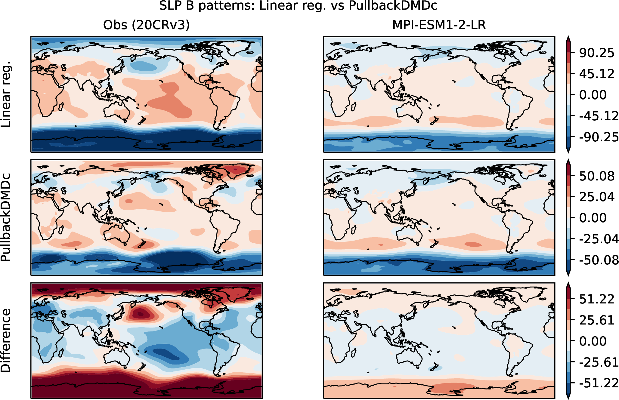
Figure 12: Spatial patterns of the LR and PullbackDMDc \(\boldsymbol{B}\) matrix for (top) ocean surface air temperature (OSAT) and (bottom) sea level pressure (SLP). These patterns are the leading forcing footprint derived from observations (left) and the ensemble-mean footprint from MPI-ESM (right). Amplitudes are not directly comparable across panels; the patterns reflect the spatial structure of the estimated forced response rather than its magnitude. Compared to LR, PullbackDMDc produces a weaker forcing signal with a distinct spatial structure, with differences that are more pronounced for SLP than OSAT..


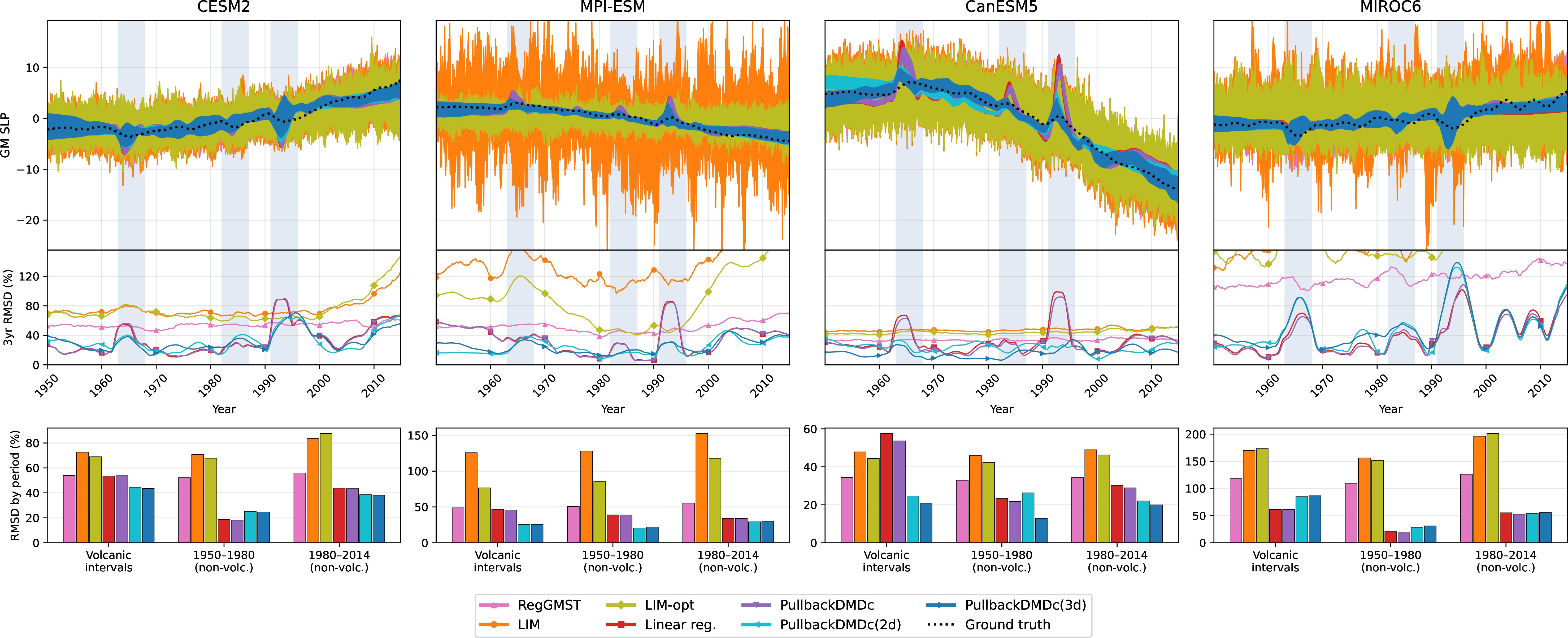


Figure 15: Same as in Fig. 2 (main text), but for SLP (top), SAT (middle), OSAT (bottom) on a short interval (\(1950-2014\)). Since this analysis covers a shorter period, there are only three volcanic intervals. The overall qualitative behavior is similar to the longer record, with amplified inter-ensemble variability and improved baseline performance relative to PullbackDMDc.. a — Sea level pressure (SLP)., b — Surface air temperature (SAT)., c — Ocean surface air temperature (OSAT).
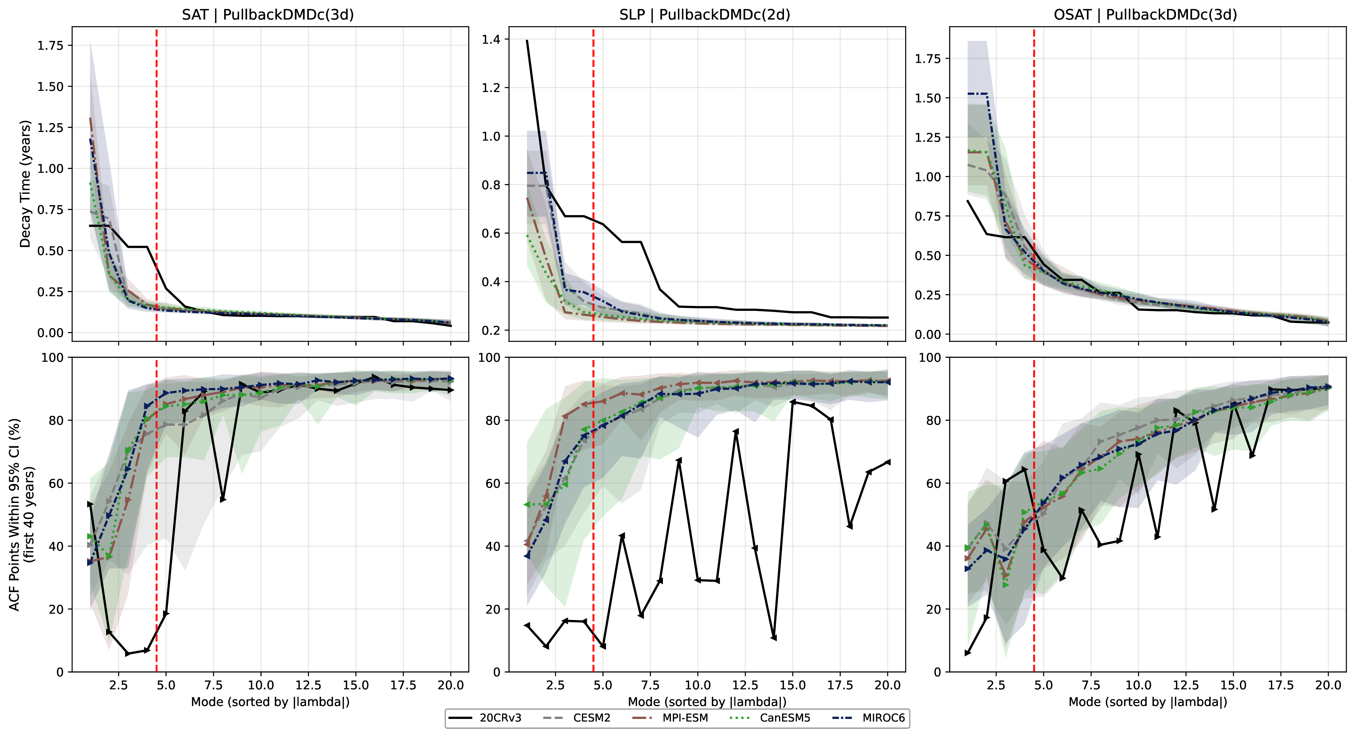


![Figure 20: Power spectral density (PSD) of the top four DMD modes for OSAT obtained from 20CRv3 reanalysis (black solid line) and four ESMs [CESM2, MPI-ESM, CanESM5, and MIROC6]. PSD estimates are computed using the multitaper method (NW = 3, K = 5 tapers) with a frequency resolution of 0.036 cy /yr (\approx28 yr period) over the 1850-2014 period. Frequency bands associated with ENSO (2–7 yr) and PDO (10–30 yr) variability are indicated. Each panel represents one mode, ordered by descending explained variance. The secondary x-axis provides equivalent periodicities. We generalize the lack of strong multidecadal variability in individual ensemble members to all ensemble members of all ESMs using the power spectral density (PSD) of the internal variability timeseries. Specifically, there are high plateaus for reanalysis (20CRv3) for timescales larger than ENSO in modes 1 and 2. These maxima are not reached by any of the top 4 modes of any ESM. The closest to reaching 10^3 is mode 4 of CanESM5.](/article/2607.18298/lag3/psd_mtm_tas_ocean_DMDc-p-3d.png "fig:")

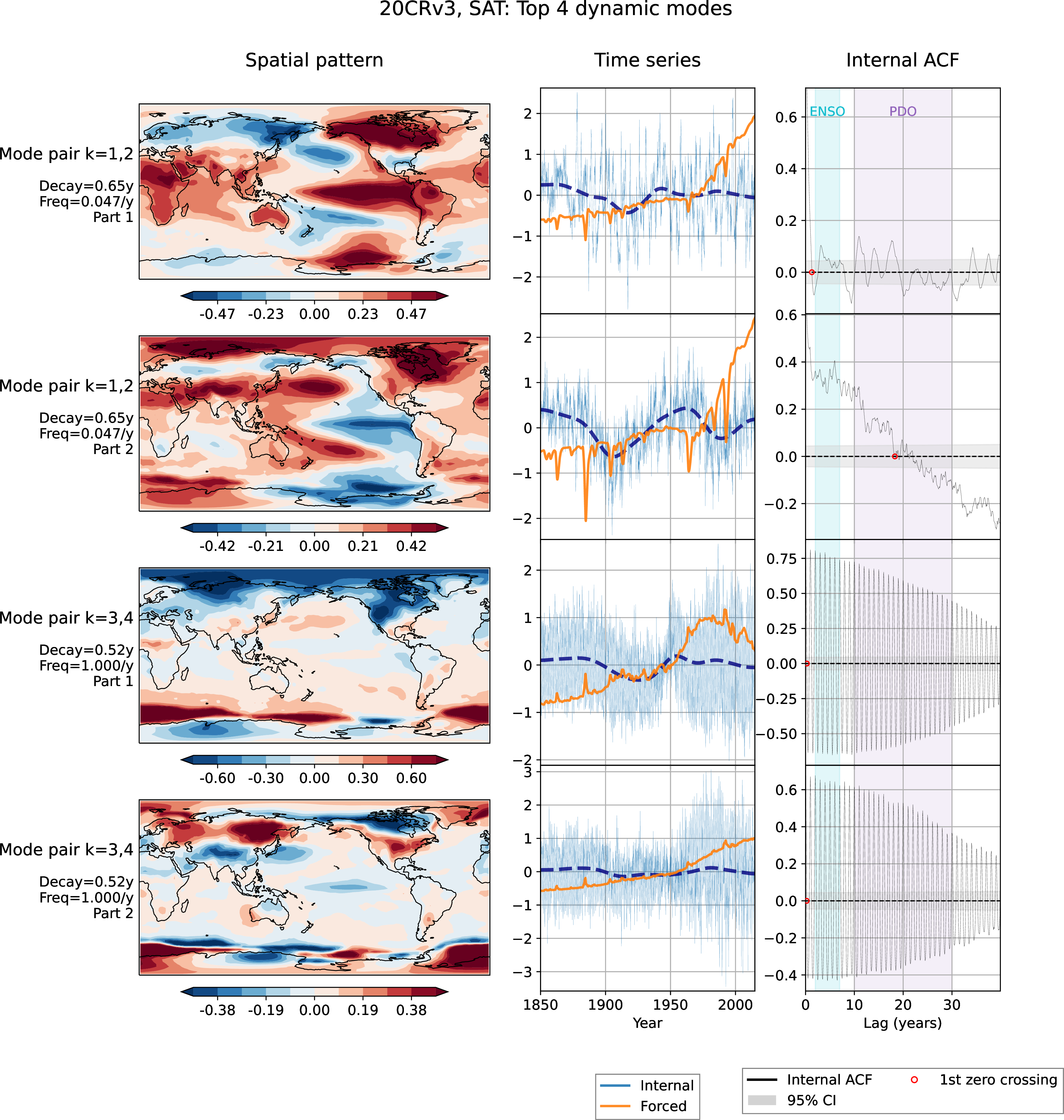

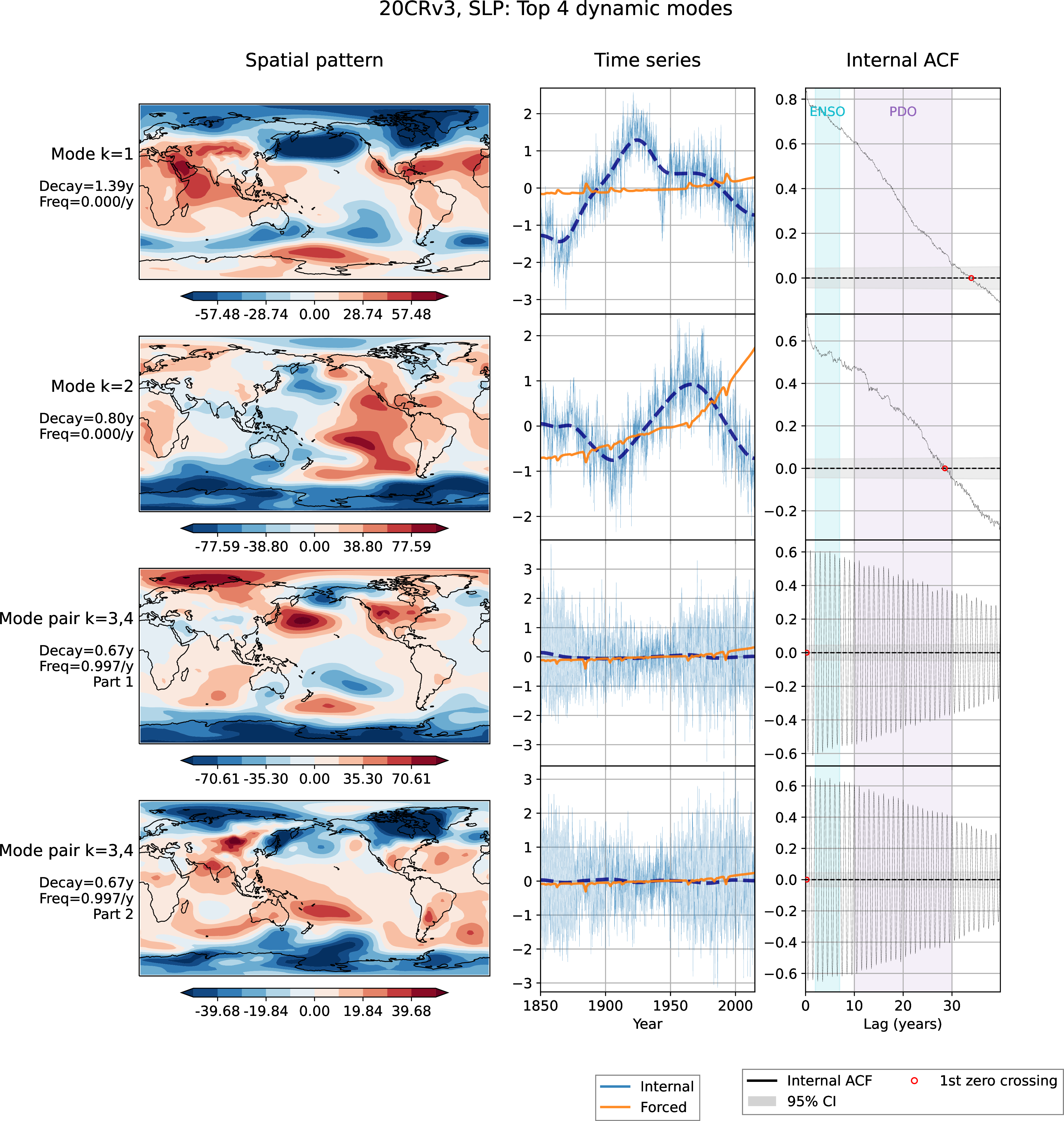

References↩︎
The noise term of a stochastic model is often called “forcing” as well. However, here we aim to separate it from our external forcing and interpret it as an approximation of internal dynamical system components.↩︎
Of course, one could also find \(\boldsymbol{x}^{(i)}(t)\) using noise \(\xi(t)\) estimated as residuals after training the model 3 .↩︎
This interval is \(1850-2014\) for the results in the manuscript. Results on a shorter interval of \(1950-2014\) are available in the Supplementary Material, Fig 4-7.↩︎