A Continual Validation, Updating, and Decision-Making Framework for
Self-Adaptive Digital Twins via Robust Model Predictive Control:
A Case Study in Additive Manufacturing
July 20, 2026
Abstract
Digital Twins rely on surrogate models to mirror physical systems in real time, yet these models can degrade as operating conditions evolve, a phenomenon known as concept drift. Maintaining surrogate fidelity under drift, particularly when models must also capture aleatoric uncertainty, remains an open challenge. Existing adaptive frameworks lack principled mechanisms for detecting when updates are needed, for efficiently adapting models from limited streaming data, and for certifying that updates genuinely improve predictive performance. Here we present an adaptive Digital Twin framework that integrates a Fisher score–based multivariate drift detector, Low-Rank Adaptation (LoRA) for parameter-efficient continual learning, and a Mann–Whitney \(U\) test for online statistical validation. The framework monitors surrogate-model confidence via Fisher score vectors, triggers targeted fine-tuning of fewer than 1% of model parameters upon drift detection, and statistically certifies predictive improvement before deploying the updated surrogate. Applied to a stochastic linear system and a directed energy deposition additive manufacturing process as case studies, the framework successfully detects distributional shifts with short delays and restores both predictive accuracy and uncertainty quantification under abrupt and incremental drift. These results establish a statistically rigorous and computationally tractable pathway for sustaining the trustworthiness of neural-network–based Digital Twins throughout their operational life cycle.
Keywords: Digital Twin; Concept Drift Detection; Continual Learning; Parameter-Efficient Fine-Tuning; Online Validation; Robust Model Predictive Control; Trustworthy Machine Learning
1 Introduction↩︎
1.1 Challenges of Maintaining Model Accuracy for Digital Twins↩︎
A Digital Twin is a virtual representation of a physical system that continuously synchronizes with its physical counterpart through bidirectional data exchange, reflecting the current state, history, and anticipated behavior of the system [1]–[4]. By assimilating streaming sensor data, it supports real-time state estimation and multi-step prediction for informed decision-making under uncertainty [5]–[7], including performance optimization [8], fault diagnosis [9], predictive maintenance [10], [11], and adaptive control [12]. Recent advances in machine learning provide expressive, data-driven surrogates of complex nonlinear dynamics [13]–[15], enabling rapid evaluation of “what-if” scenarios without costly high-fidelity simulation [5], [16] and turning Digital Twins from static monitors into proactive, intelligent systems.
When integrated with decision-making frameworks such as dynamic programming [11], reinforcement learning (RL) [17], [18], or model predictive control (MPC) [8], the Digital Twin becomes a closed-loop, real-time optimization engine in which the surrogate is the predictive core subject to operational constraints and safety requirements [19]. Unlike feedback control that relies on error correction, such frameworks perform proactive optimization over a horizon. MPC’s receding-horizon structure [20], [21] complements this paradigm: at each step the virtual twin supplies state estimates and predictions, MPC solves a constrained optimization for control actions [6], [8], and continual re-optimization adapts to disturbances and evolving conditions.
MPC’s repeated real-time optimization places stringent demands on model efficiency, so conventional formulations often rely on linear state-space models solved via convex quadratic programming (QP) [22]–[24]. Increasingly, neural networks (NNs) and other nonlinear approximators surrogate complex dynamics [25]–[28], expanding MPC to highly nonlinear, spatio-temporal processes and broadening Digital Twin systems. Crucially, the availability of accurate global rather than merely local models lets the virtual twin faithfully mirror the physical entity and support reliable system-level prediction and decision-making. The effectiveness of model-based decision-making depends critically on model fidelity [29], so the virtual and physical systems must remain synchronized. In practice, partial and noisy observations, unmeasured disturbances, and latent material or environmental variations [30] produce model-plant mismatch through parameter variation [31], unmodeled dynamics [32]–[34], structural simplification [35], or degradation [36]. Static models therefore drift out of alignment, motivating methods that update the model during operation.
Although adaptive MPC with continuous model updating has been widely applied [37], [38], its transition to learning-based MPC still faces challenges regarding model trustworthiness. Unlike conventional MPC, where linear models are commonly used and can be readily updated via a Kalman filter [39] or recursive least squares [40], updating a black-box data-driven model, in particular, a deep neural network (DNN), in real time is challenging in three ways:
When to update the model: For learning-based predictive models, particularly DNNs, updating at every time step can introduce substantial computational overhead and a risk of overfitting, potentially hindering real-time implementation and stability. Conversely, infrequent updates may delay the response to distributional drift, leading to performance degradation and reduced robustness [41]. A principled mechanism is therefore needed to determine when model updates should be triggered, balancing computational efficiency with adaptability to evolving system dynamics.
How to update the model: Updating a highly parameterized model, such as a DNN with numerous tunable weights, from limited streaming data is inherently challenging. In particular, when the incoming data undergo abrupt changes or contain measurement noise, naive iterative fine-tuning can cause unstable adaptation, overfitting to corrupted samples, or catastrophic forgetting, i.e., erosion of previously acquired knowledge and degradation of performance on previously well-modeled operating regimes. Data- and parameter-efficient fine-tuning strategies are therefore needed for DNN-based MPC.
Is the update successful: Digital Twins must be continuously validated throughout their operation and life cycle [2], particularly when the virtual counterpart relies on a data-driven model updated from limited batches of streaming data. Given the aforementioned risks, deploying an inadequately validated updated model for safety-critical decision-making can lead to severe performance degradation or even system-level failure. Systematic post-update validation is therefore indispensable to ensure reliability and trustworthiness.
1.2 When to Update the Digital Twin?↩︎
1.2.1 Updating Models in Existing Model-Based Control Methods↩︎
Determining when to update the model in real time intelligently remains an open challenge [42], [43]. Update strategies are broadly instance-wise, batch-wise, periodic, or event-triggered. Instance-wise schemes update at every step via gradient corrections [44]–[47], recursive least squares [45], or online Gaussian-process updates [32], [48]. These are responsive but raise memory cost and degrade long-term recall [49], motivating cost-aware updating [41]. Batch-wise and periodic schemes retrain after a fixed number of samples [50], [51] or at a fixed interval [52], sometimes with threshold-based retraining of lightweight models [53], [54]. These improve efficiency but can delay the response to abrupt changes. Event-triggered schemes update only when drift is detected [55]. For example, Lyapunov-based MPC activates updates when stability conditions or prediction-residual triggers are violated [46], but such designs are limited to low-dimensional outputs and are hard to generalize to multi-output Digital Twins.
Existing adaptive-MPC work emphasizes trade-offs among adaptation frequency, overhead, memory, and performance, but rarely links model trustworthiness to a drift detector that signals when accuracy degrades. Such triggering is straightforward for classification (via accuracy thresholds [49]) yet far less intuitive for regression, leaving a unified update-timing framework for Digital Twins underexplored.
1.2.2 Concept Drift Detection↩︎
Beyond MPC, formal mechanisms for detecting “when the model fails” have been studied extensively in the context of concept drift detection [56]–[58]. Let \(\mathcal{D}_t = \{(x_i, y_i)\}_{i=1}^{n}\) denote the joint data distribution at time \(t\), where \(x \in \mathbb{R}^d\) is the input vector and \(y \in \mathbb{R}^m\) is the output. Concept drift refers to a change in the distribution \(P_t(x, y)\) over time [56]: \[\exists\, t_0 < t_1 : \quad P_{t_0}(x, y) \neq P_{t_1}(x, y). \label{eq:drift95def}\tag{1}\]
In practice, the broad family of drifts can originate from a shift in the input marginal distribution \(p_t(x)\) only (covariate shift), a change in the conditional output distribution \(p_t(y \mid x)\) (concept drift), or both simultaneously. In this work, we are only focusing on concept drift, where the relationship between the input and the output has changed.
The most common detectors monitor prediction error, e.g.the Drift Detection Method (DDM) [59], the Exponentially Weighted Moving Average (EWMA) [60], and the Cumulative Sum (CUSUM) [61], which are efficient for streaming data but inherently univariate, offer limited diagnosis, and lose sensitivity when a distributional change does not immediately raise the error, as under incremental drift or covariate shift [62]. Distribution-based methods compare a reference and a current window, e.g.Adaptive Windowing (ADWIN) [63], Maximum Mean Discrepancy (MMD) [64], and the Kolmogorov–Smirnov test, but scale poorly with dimensionality and, relying on local windows, struggle with incremental drift [53], [54]. Zhang and Apley [62] instead track the Fisher score vector, i.e. the gradient of the log-likelihood with respect to the parameters, enabling parameter-level attribution of not only when drift occurs but which parts of the input–output relationship changed, providing a principled, interpretable fit with NN-based Digital Twins.
Most existing detectors, however, assume that operation can be halted and the detector reinitialized on identified “normal” data [65], which is impractical for autonomous, continuously operating Digital Twins and anchors the detector to outdated concepts. This motivates continual, data-efficient online re-initialization and, more broadly, the integration of formal drift detection with continual decision-making as a critical element for proactive, drift-aware decision-making in Digital Twins.
1.3 How to Update the Digital Twin?↩︎
1.3.1 Catastrophic Forgetting and Continual Learning↩︎
Once drift is detected, adapting the virtual twin to a new distribution must accommodate evolving dynamics while avoiding overfitting to limited streaming data and undesirable loss of useful prior structure [53], [66], [67]. Catastrophic forgetting is studied under continual learning, where regularization-, replay-, optimization-, and representation-based methods mitigate forgetting. These mostly preserve performance across multiple tasks, whereas under concept drift, the aim is rather to overwrite outdated knowledge for plasticity. Here, “forgetting” for the purpose of adapting to new concepts means erasing still-relevant structural representations (i.e., the physics or the pre-trained network as the backbones) and degrading robustness.
Recent advances in parameter-efficient fine-tuning (PEFT) provide a promising direction for efficient model updating from streaming data [68]. PEFT methods adapt large NNs by updating only a subset or a low-dimensional subspace of the parameters, reducing computational cost while improving training stability. Among these, Low-Rank Adaptation (LoRA) [69] is a representative reparameterization-based technique that introduces trainable low-rank matrices in parallel to the pretrained weights, offering parameter efficiency, low inference latency, and stable optimization. Despite their success in large-scale learning tasks, to the best of our knowledge, the application of such methods to NN-based model adaptation for dynamical systems and the real-time decision-making of Digital Twins has not yet been investigated.
1.3.2 Adaptation in MPC and Digital Twins↩︎
From a control-design perspective, adaptive MPC can be realized in three principal forms [70]. The first updates the predictive model directly via online system identification [71]. The second adapts controller parameters, such as tuning the weighting matrices in nonlinear MPC [72] or analytically adjusting the control horizon [73], without modifying the underlying model. The third integrates RL with MPC, where RL tunes the control parameters online while preserving the MPC structure [70], [74], [75]. Related approaches further combine offline-trained deep RL with nonlinear MPC to calibrate model parameters, ensuring synchronization between the digital and physical systems [76]. In this work, the focus is placed exclusively on model-level adaptation, as it directly determines the fidelity between the virtual twin and the physical system.
Model-level adaptation typically estimates parameters under uncertainty via optimization [77], recursive least squares [78], Kalman filtering [29], [31], [79], or divergence-based correction [36], with AM applications calibrating temperature-dependent properties [80] or Koopman models [12]. Naive recursive estimation, however, risks instability and overfitting to streaming data, yielding only locally accurate models rather than global ones.
To mitigate overfitting and forgetting, several strategies constrain updates to specific components: residual learning of physics–data discrepancies [32], [81]–[83], layer-wise online updating [84], and adaptive bias correction [82]. These methods all fine-tune the model by preserving the pretrained structure and minimizing the number of tunable parameters, highlighting the importance of data- and parameter-efficient fine-tuning. Motivated by these works, the present work advocates integrating PEFT-based methods into Digital Twin adaptation, particularly when NNs are used as surrogates, enabling controlled, efficient, and robust model updates from limited streaming data while balancing plasticity and stability.
1.4 Is the Update Successful?↩︎
In safety-critical and high-consequence systems, model updating must be accompanied by systematic validation to ensure that adaptation truly improves, rather than degrades, predictive and control performance. In the context of trustworthy scientific machine learning, verification and validation (V&V) are regarded not as one-time procedures but as iterative processes of credibility assessment spanning problem formulation, model development, deployment, and domain shift [85]. In particular, distributional shift between the training and operational domains necessitates continuous validation to maintain model reliability.
Yet most works evaluate updates offline or retrospectively, e.g.via held-out transfer-learning performance [51] or post-hoc classification tests [86], which benchmark accuracy but do not safeguard real-time updating in closed-loop systems or guarantee stability and constraint satisfaction during deployment. A notable exception is the Lyapunov-based MPC of [46], which gates updates on stability conditions and accumulated-error triggers. Overall, real-time validation mechanisms that assess model performance after updating, at test time, remain scarce. Developing principled criteria to certify the success of model updates in Digital Twin systems is therefore an important research direction.
1.5 Research Objective↩︎
A central research gap lies in the absence of a trustworthy framework that enables Digital Twins to support real-time decision-making while remaining reliable and adaptive throughout their life cycle. Although machine-learning–enabled MPC has substantially improved predictive accuracy for control, most existing efforts concentrate on local model performance and overlook the statistical rigor required for drift detection and systematic validation of continuously updated models. This deviates from the purpose of a Digital Twin, whose target is to maintain the faithfulness of the virtual model to the physical system, not solely to solve a control problem well. From a trustworthy-AI perspective, updating models without structured validation raises fundamental concerns regarding credibility and safety. While the control community has traditionally emphasized performance and stability, the statistical-learning literature has long recognized drift management and validation as essential components of adaptive systems. This reveals a critical gap at the intersection of drift detection, continual learning with validation, and real-time decision-making—a gap that is central to the reliability and safe operation of Digital Twins over their life cycle.
To the best of our knowledge, no existing framework simultaneously addresses the following three challenges:
how to integrate drift detection into real-time decision-making frameworks with principled online reset and adaptation mechanisms for multivariate NN surrogate models, providing insight into when distributional shifts occur;
how to conduct streaming-data continual learning in a parameter- and data-efficient manner; and
how to embed online validation within continual learning to safeguard adaptation and improve model trustworthiness.
To address these challenges, we propose an adaptive Digital Twin framework for handling concept drift in real-time decision-making, as illustrated in Figure 1. Building upon our prior work on uncertainty-aware Digital Twins [6], which represents a closed-loop Digital Twin system (left-hand side of Figure 1), the present work extends this architecture with a generalized adaptation layer (right-hand side of Figure 1) that can be implemented across NN-based Digital Twin systems. The key distinction from existing work is that our framework embeds an additional level of uncertainty awareness and validation to ensure that the model is fine-tuned successfully and automatically.
![Figure 1: The proposed framework for the Adaptive Digital Twin. The gray box and the blue box on the left-hand side were proposed in our previous work [6], and the green box on the right-hand side highlights the novelty of this work. The illustration also shows that the proposed method can serve as a non-intrusive add-on to existing Digital Twin frameworks.](/article/2607.18164/figures/overall_framework.png "fig:")
The primary contribution of this work lies not in the individual components but in their principled integration into a unified framework that systematically couples drift detection, continual learning, and statistical validation within real-time decision-making, forming a comprehensive pipeline for the continual adaptation of NN-based Digital Twins that maintains both predictive accuracy and trustworthiness throughout the operational life cycle, even in the presence of previously unseen distributional shifts. The selected methods and implementations for each module are further designed to maximize generalizability, ensuring broad applicability across NN-based Digital Twin systems beyond the specific architectures and case studies considered here. Specifically, the contributions of this work are as follows:
Novel drift-detection mechanism — determining when to update the model: A Fisher score–based multivariate drift-detection method is developed to identify concept drift in NN surrogate models during Digital Twin operation. Novel real-time implementations are introduced, including diagonal covariance approximation and threshold estimation via bootstrapping, making the approach computationally tractable for online deployment. The method is model-agnostic and applicable to general supervised-learned, differentiable models, providing detection capability on concept drift.
Parameter-efficient fine-tuning — determining how to update the model: To the best of our knowledge, this is the first work to introduce LoRA as a parameter- and data-efficient fine-tuning strategy for online surrogate-model adaptation in Digital Twin systems and adaptive MPC governed by highly nonlinear dynamics, enabling rapid updates from limited streaming data while mitigating catastrophic forgetting. Through benchmarking against existing methods, we show that LoRA is competitive with, and in the settings considered slightly superior to, head and hybrid fine-tuning, and we adopt it as the default fine-tuning method within the proposed framework.
Online validation — determining whether the update is successful: An online validation procedure based on the Mann–Whitney \(U\) test is introduced to statistically assess whether the adapted model achieves a significant reduction in predictive loss relative to the current live model. This nonparametric, distribution-free test ensures that model replacement is justified by measurable predictive improvement, providing a principled safeguard against deploying an inadequately updated surrogate.
The rest of the paper is organized as follows. Section 2 reviews the technical foundations of the underlying closed-loop Digital Twin, including MPC and its robust extension, surrogate modeling via TiDE, and uncertainty-aware learning through quantile regression. Section 3 presents the proposed Adaptive Digital Twin framework, introducing Fisher score–based drift detection and LoRA together with their online implementations, and detailing their integration with robust MPC for continual decision-making under evolving operating conditions. Section 4 evaluates the effectiveness of LoRA-based online model adaptation and the proposed validation procedure through a series of benchmark studies. Section 5 demonstrates the complete framework on a real-world directed energy deposition (DED) Digital Twin operating under concept drift. Finally, Section 6 summarizes the main findings and current limitations, and outlines directions for future research.
2 Technical Background↩︎
This section reviews the three building blocks of the closed-loop, uncertainty-aware Digital Twin upon which the proposed framework is constructed: decision-making through MPC and its robust extension, surrogate modeling of dynamical systems via the Time-series Dense Encoder (TiDE), and quantile regression for uncertainty-aware learning.
2.1 Model Predictive Control and Robust Model Predictive Control↩︎
MPC is a constrained optimal control method that repeatedly solves a finite-horizon optimization problem using an explicit prediction model of the system [87]. At each sampling instant, the controller predicts the future system evolution over a horizon of length \(N\), computes an optimal control sequence by minimizing a cost functional subject to dynamic and operational constraints, implements only the first control input, and then shifts the horizon forward, as illustrated in Figure 2 (a) and Figure 2 (b). This receding-horizon mechanism provides inherent feedback and enables the handling of multivariable interactions and constraints.

2.1.0.1 System model.
Consider a discrete-time nonlinear system \[\mathbf{x}_{k+1} = f(\mathbf{x}_k, \mathbf{u}_k), \label{eq:dyn95sys}\tag{2}\] where \(\mathbf{x}_k \in \mathbb{R}^n\) is the state vector and \(\mathbf{u}_k \in \mathbb{R}^m\) is the control input at time step \(k\). The mapping \(f: \mathbb{R}^n \times \mathbb{R}^m \to \mathbb{R}^n\) describes the system dynamics. In practice, the controller employs a predictive model \(\hat{f}\), which may be physics-based, data-driven, or hybrid.
2.1.0.2 Finite-horizon optimal control problem.
Given the current state measurement \(\mathbf{x}_k\) and a reference trajectory \(\mathbf{r}_{k+1:k+N}\), the MPC problem at time \(k\) is formulated as \[\begin{align} \min_{\mathbf{u}_{k:k+N-1}} \quad & J_k = \sum_{i=1}^{N} \left\| \hat{\mathbf{x}}_{k+i} - \mathbf{r}_{k+i} \right\|_{\mathbf{Q}}^2 + \sum_{i=0}^{N-1} \left\| \mathbf{u}_{k+i} \right\|_{\mathbf{R}}^2 \label{eq:mpc95cost95new} \\ \text{s.t.} \quad & \hat{\mathbf{x}}_{k} = \mathbf{x}_k, \\ & \hat{\mathbf{x}}_{k+i+1} = \hat{f}(\hat{\mathbf{x}}_{k+i}, \mathbf{u}_{k+i}), \quad i = 0,\dots,N-1, \\ & \hat{\mathbf{x}}_{k+i} \in \mathbb{X}, \quad i = 1,\dots,N, \\ & \mathbf{u}_{k+i} \in \mathbb{U}, \quad i = 0,\dots,N-1, \\ & \mathbf{g}(\hat{\mathbf{x}}_{k+i}, \mathbf{u}_{k+i}) \le 0, \\ & \mathbf{h}(\hat{\mathbf{x}}_{k+i}, \mathbf{u}_{k+i}) = 0. \end{align}\tag{3}\] The quadratic norm is defined as \(\|\mathbf{z}\|_{\mathbf{Q}}^2 = \mathbf{z}^\top \mathbf{Q} \mathbf{z}\), with weighting matrices \(\mathbf{Q} \succ 0\) and \(\mathbf{R} \succ 0\) that balance tracking accuracy and control effort. The admissible state and input sets are denoted by \(\mathbb{X}\) and \(\mathbb{U}\), respectively. The functions \(\mathbf{g}(\cdot)\) and \(\mathbf{h}(\cdot)\) represent general inequality and equality constraints, which may encode actuator limits, safety requirements, and physical coupling relationships. The optimization problem is solved at each time step, yielding an optimal sequence \(\mathbf{u}_{k:k+N-1}^\star\). Only \(\mathbf{u}_k^\star\) is applied to the plant, and the procedure is repeated at the next sampling instant with updated state information. For linear dynamics and quadratic objectives with convex constraints, the problem reduces to a quadratic program. For nonlinear models, it leads to a nonlinear program that must be solved efficiently to satisfy real-time requirements.
2.1.0.3 Robust MPC.
In practical applications, system evolution is affected by disturbances, modeling errors, and parametric uncertainties. A more general representation of the dynamics is \[\label{eq:stochastic95system} \mathbf{x}_{k+1} = f_w(\mathbf{x}_k, \mathbf{u}_k, \mathbf{w}_k),\tag{4}\] where \(\mathbf{w}_k \in \mathbb{R}^p\) denotes an exogenous disturbance. The disturbance can be characterized either deterministically, \[\mathbf{w}_k \in \mathbb{W},\] with \(\mathbb{W}\) a bounded uncertainty set, or probabilistically, \[\mathbf{w}_k \sim \mathcal{N}(\mathbf{0}, \boldsymbol{\Sigma}_w),\] where \(\boldsymbol{\Sigma}_w\) is the disturbance covariance matrix. Conventional MPC typically employs a nominal model and does not explicitly guarantee constraint satisfaction under uncertainty. Robust MPC extends the formulation by accounting for the impact of disturbances on state predictions and constraints. Using a surrogate model \(\hat{f}_w\) trained on data that may contain noise and unmodeled effects, a robust counterpart can be expressed as \[\begin{align} \min_{\mathbf{u}_{k:k+N-1}} \quad & J_k = \sum_{i=1}^{N} \left\| \hat{\mathbf{x}}_{k+i} - \mathbf{r}_{k+i} \right\|_{\mathbf{Q}}^2 + \sum_{i=0}^{N-1} \left\| \mathbf{u}_{k+i} \right\|_{\mathbf{R}}^2 \\ \text{s.t.} \quad & \hat{\mathbf{x}}_{k} = \mathbf{x}_k, \\ & \hat{\mathbf{x}}_{k+i+1} = \hat{f}_w(\hat{\mathbf{x}}_{k+i}, \mathbf{u}_{k+i}), \\ & \hat{\mathbf{x}}_{k+i} \in \mathbb{X}, \\ & \mathbf{u}_{k+i} \in \mathbb{U}, \\ & \mathbf{g}(\hat{\mathbf{x}}_{k+i}, \mathbf{u}_{k+i}) \le 0, \\ & \mathbf{h}(\hat{\mathbf{x}}_{k+i}, \mathbf{u}_{k+i}) = 0, \end{align}\] for \(i = 0,\dots,N-1\) where appropriate. Depending on the uncertainty description, robust MPC may enforce worst-case constraint satisfaction over \(\mathbb{W}\), propagate uncertainty sets along the prediction horizon, or impose chance constraints that ensure probabilistic feasibility. In data-driven settings, the predictive model \(\hat{f}_w\) does not receive the disturbance \(\mathbf{w}_k\) explicitly during online prediction. Instead, its influence is implicitly captured through training data, uncertainty-quantification mechanisms, or distributionally robust reformulations. This uncertainty-aware extension enhances reliability and safety in the presence of model mismatch and stochastic perturbations, which is particularly critical in safety-constrained, real-time decision-making applications. For instance, tube-based MPC can solve robust MPC problems by explicitly identifying the actual state region surrounding the nominal trajectory (the tube), illustrated in Figure 2 (c). In this work, we implement a data-driven version of tube-based robust MPC proposed by [6], elaborated in Section 3.2.
2.2 Time-Series Dense Encoder↩︎
The surrogate must support fast inference for repeated MPC evaluations and accommodate exogenous control inputs [6]. We adopt TiDE [88], the Time-series Dense Encoder, an encoder–decoder of stacked linear residual blocks that attains competitive accuracy while being 5–10\(\times\) faster at inference than Transformer counterparts. Moreover, it supports simultaneous multi-step prediction, avoiding error propagation while learning temporal dependencies, which suits partially observable systems and parallelizes the prediction of future state trajectories.
![Figure 3: The network structure of Time Series Dense Encoder (TiDE), modified from [88]](/article/2607.18164/figures/TiDE.png "fig:")
TiDE encodes the full look-back window and covariates into a compact latent representation and decodes the entire horizon in a single forward pass (Figure 3), avoiding the sequential unrolling of autoregressive models and the quadratic cost of self-attention while filtering noise through its low-dimensional bottleneck. TiDE separates targets (the predicted states) from covariates (auxiliary time-varying inputs that condition but are not predicted), the latter split into past covariates (observed over the look-back window) and future covariates (known over the horizon). This maps naturally onto a control-exogenous dynamical system whose state evolution depends on its history and on applied inputs and prescribed conditions. Specifically, TiDE takes past states \(\mathbf{x}_{k-w+1:k}\) as the past target, past inputs \(\mathbf{u}_{k-w:k-1}\) and conditions \(\{\mathbf{u}_{k-w:k-1},\mathbf{d}_{k-w:k-1}\}\) as past covariates, and planned future inputs and conditions \(\{\mathbf{u}_{k:k+N-1},\mathbf{d}_{k:k+N-1}\}\) as future covariates, producing future states predictions \(\hat{\mathbf{x}}_{k+1:k+N}\) (Figure 4), where \(\mathbf{d}\) are prescribed process parameters and \(\mathbf{u}\) the inputs optimized by the MPC. The surrogate is \[\begin{align} \hat{\mathbf{x}}_{k+1:k+N} = \boldsymbol{TiDE}(\mathbf{x}_{k-w+1:k},& \;\mathbf{d}_{k-w:k-1},\; \mathbf{u}_{k-w:k-1}, \mathbf{d}_{k:k+N-1},\; \mathbf{u}_{k:k+N-1} \mid \boldsymbol{\theta}), \label{eq:TiDE95general} \end{align}\tag{5}\] where \(\boldsymbol{\theta}\) collects all trainable parameters, allowing the MPC optimizer to query TiDE with candidate input sequences for simultaneous \(N\)-step predictions without sequential unrolling.

2.3 Quantile Regression↩︎
In engineering applications, a predictive model that returns only a single point estimate of future system states is often insufficient for robust decision-making, as it gives no indication of how reliable that estimate is under disturbances. Quantile regression [89]–[91] addresses this limitation by predicting conditional quantiles rather than the mean, yielding distribution-free prediction bounds that represent aleatoric uncertainty and accommodate heteroscedasticity without assuming an error distribution. The loss function for a given quantile level \(q \in (0, 1)\) and response channel \(j\in{1,...,N_d}\) is defined as \[L_{q,j}(x_{j,t}, \hat{x}_{j,t}) = \begin{cases} q \cdot (x_{j,t} - \hat{x}_{j,t}), & \text{if } x_{j,t} \geq \hat{x}_{j,t}, \\ (1 - q) \cdot (\hat{x}_{j,t} - x_{j,t}), & \text{if } x_{j,t} < \hat{x}_{j,t}, \end{cases} \label{eq:standard95quantile}\tag{6}\] where \(x_t\) and \(\hat{x}_t\) are the ground-truth and predicted values at time \(t\), respectively. The asymmetric weighting on the two residual terms encourages the model’s output to converge to the \(q\)-th percentile of the conditional distribution: setting \(q = 0.5\) recovers the median, while \(q = 0.1\) and \(q = 0.9\) yield the lower and upper bounds of an 80% prediction interval. By training TiDE simultaneously across multiple quantile levels using the aggregate of the \(L_{q,j}\) losses, the framework produces interval predictions of future system states that can be directly propagated through the MPC formulation to enable uncertainty-aware control [6], [8], [91]. The aggregated quantile loss function across all channels and for multi-step-ahead prediction can therefore be denoted as: \[L_Q(\mathbf{x}_{k+1:k+N},\mathbf{\hat{x}}_{k+1:k+N})= \sum_{q=1}^{N_q}\sum_{j=1}^{N_d}\sum_{i=k+1}^{k+N}L_{q,j}(x_{i,j},\hat{x}_{i,j})\]
Together, these three components form the uncertainty-aware, closed-loop Digital Twin developed in our prior work [6]: TiDE provides a fast multi-step surrogate, quantile regression supplies distribution-free uncertainty bounds, and robust MPC translates these bounds into safe control actions. However, this framework assumes that the surrogate remains faithful to the physical system. When operating conditions drift, the learned quantiles, and thus the safety margins used by robust MPC, may no longer be valid. The next section introduces the proposed adaptation layer, which detects drift, efficiently updates the surrogate using streaming data, and statistically validates each update before reintegrating it into the decision-making loop.
3 The Proposed Method↩︎
This section presents the proposed Adaptive Digital Twin framework, summarized in Figure 1. Building on the closed-loop components reviewed in Section 2, the presentation is organized around the three questions posed in the Introduction: Section 3.3 introduces Fisher score–based drift detection and its online implementation to answer when to update the model, Section 3.4 introduces LoRA and the batch-wise fine-tuning procedure built around it to answer how to update the model, and Section 3.5 presents the statistical validation that determines whether an update is successful and may replace the live model. We make two assumptions on the drift that the physical system encounters:
Assumption 1. The physical system encounters only abrupt drift and incremental drift, which are not reoccuring and infrequent.
Assumption 2. Following the characterization of drift as either abrupt or gradual, it is assumed that, after model adaptation, the system does not experience an immediate subsequent drastic drift. In other words, drift evolves on a timescale that allows the updated model to remain valid for a non-negligible period.
These assumptions reflect the physics and operating limits of engineered systems. Behavior changes arise from discrete events (faults, regime switches) or continuous processes (wear, aging, thermal effects), giving abrupt and incremental drift respectively, with complex patterns interpretable as combinations of the two. Abrupt events are infrequent owing to limited failure rates, while incremental drift cannot induce successive large deviations, and monitoring/control systems should stabilize operation after each correction. Statistically, this enforces a separation of timescales between drift and adaptation, ensuring the updated model stays valid long enough for reliable estimation, validation, and decision-making. Even if rapid successive drift occurs, the validation gate simply withholds deployment, and the framework keeps re-adapting on fresh data, so a violated assumption costs responsiveness but does not push an unvalidated model into the safety-critical loop.
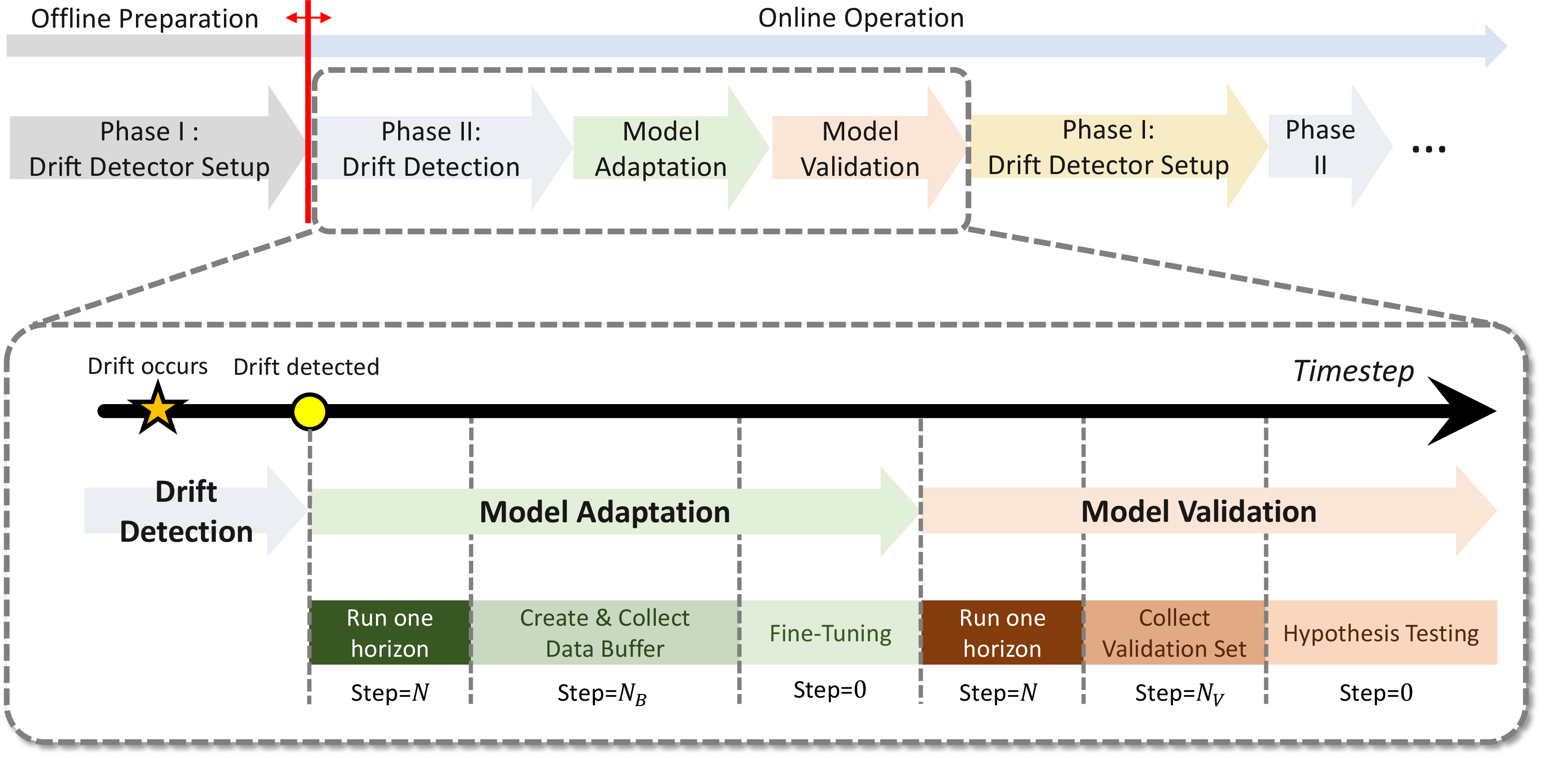
3.1 Offline Model Training↩︎
Data are collected to train an offline, pretrained predictive model with using TiDE (Section 2.2) with quantile regression (Section 2.3), simultaneously predicting the median and the upper (0.95) and lower (0.05) quantiles for uncertainty-aware prediction. The parameters of the pretrained model are then frozen, with LoRA layers (Section 3.4.1) appended to all layers for efficient adaptation. If the network lacks a dedicated final linear layer for score monitoring (Section 3.3.3), an identity-initialized linear layer \(\mathbf{W}_{\text{lin}}\) is added as the output layer, leaving predictions unchanged, and set as the only gradient-tracked parameters, isolating the Fisher-score computation to \(\mathbf{W}_{\text{lin}}\). The augmented model becomes the live model, with an identical idle copy.
3.2 Continual Decision-Making with Multi-Step Robust Model Predictive Control↩︎
For uncertainty-aware decision-making, we adopt the simultaneous multi-step robust MPC framework of [6]. This approach integrates multi-step-ahead predictions with deep quantile learning to reformulate the stochastic MPC problem into a tractable deterministic optimization while retaining probabilistic guarantees. Through its receding-horizon formulation, the MPC continually updates and resolves the control problem using the latest state measurements from the physical system, enabling the Digital Twin to provide adaptive and optimal decisions in real time.
Consider a nonlinear dynamical system subject to stochastic disturbances as described in Equation 4 . The robust MPC optimizes the control inputs over a finite horizon while satisfying probabilistic constraints on the system states: \[\min_{u} \;\mathbb{E}[J(u, x, r, w)], \quad \text{s.t. } \Pr(x_{k+i} \in \mathcal{X}) \ge \alpha, \;\forall i, \quad u_{k+i} \in \mathcal{U}.\] However, directly solving this problem is computationally intractable due to uncertainty propagation and the evaluation of probabilistic constraints. In this work, we leverage a multi-step predictor via TiDE, \(\hat{\mathbf{x}}_{k+1:k+N}=[\bar{\mathbf{x}}_{k+1:k+N},\tilde{\mathbf{x}}_{k+1:k+N},\underline{\mathbf{x}}_{k+1:k+N}]\), to directly predict the future-state distribution through learned quantiles, where \(\bar{x},\underline{x}\) are the upper/lower quantiles at confidence level \(\alpha\). Each chance constraint is then enforced deterministically on the predicted quantile, e.g.\(\Pr(x_{j,k+i}\le x_j^{\mathrm{ub}})\ge\alpha \Leftrightarrow \bar{x}_{j,k+i}\le x_j^{\mathrm{ub}}\) (and analogously for the lower bound), reducing the stochastic MPC to the deterministic problem \(\min_{v} J(v,\tilde{x},r)\) subject to \(\bar{x}_{k+i}(v)\le x^{\mathrm{ub}}\) and \(\underline{x}_{k+i}(v)\ge x^{\mathrm{lb}}\) for all \(i\), with the \(v\)-dependence entering through the predictive model. The aleatoric uncertainty is thus handled explicitly through the learned bounds, avoiding sample-based approaches (Monte Carlo dropout, Bayesian NNs) and iterative uncertainty propagation in which error may accumulate [92]. Moreover, an ancillary feedback policy \(u_k=v_k+Ke_k\), \(e_k=x_k-\tilde{x}_k\), is added and the input set tightened to \(v_{k+i}\in\mathcal{U}\ominus K\mathcal{Z}_{k+i}\), where \(v_{k+1}\) is the control input applied to the system by correcting \(u_{k+1}\), and \(\mathcal{Z}_{k+i}\) is the quantile interval, ensuring feasibility under disturbances. Through this reformulation, the uncertainty-aware MPC problem is converted into a deterministic optimization problem that can be solved efficiently in real time while maintaining probabilistic guarantees on constraint satisfaction via the learned quantile bounds. The reader may refer to [6] for more details on the multi-step robust MPC.
3.3 When to Update the Digital Twin? – Score-Based Drift Detection↩︎
The first module of the framework determines when the surrogate must be updated, by monitoring whether newly observed data remain consistent with the distribution learned by the fitted model. We adopt the score-vector–based framework of [62], which offers a multivariate, model-agnostic mechanism for this assessment. By measuring the sensitivity of the log-likelihood with respect to the model parameters, the Fisher score quantifies how strongly new observations push the model away from its previously learned parameterization; large deviations therefore indicate potential distributional shifts, signaling that the model may need to be updated or revalidated. Unlike error-based approaches which trigger alarms only when prediction errors increase, struggle with multivariate outputs, and can miss changes in \(P(Y \mid \mathbf{X})\) that leave the error rate unchanged, the score-based method directly monitors the confidence of the fitted parameters regardless of output dimensionality. The multivariate score vector is aggregated into a single detection statistic via the Mahalanobis distance, which re-weights parameter sensitivities by their correlations, while parameter-wise score components provide additional diagnostic insight into how the drift manifests [62]. For NN-based models, the score vectors are obtained at negligible cost through backpropagation on the computation graph, making the method directly applicable in real-time settings. In the following, we first review the statistical foundation of the score-based detector (Sections 3.3.1–3.3.3) and then present its online implementation within the proposed framework (Section 3.3.4).
3.3.1 Fisher Score Vector for Parametric Models↩︎
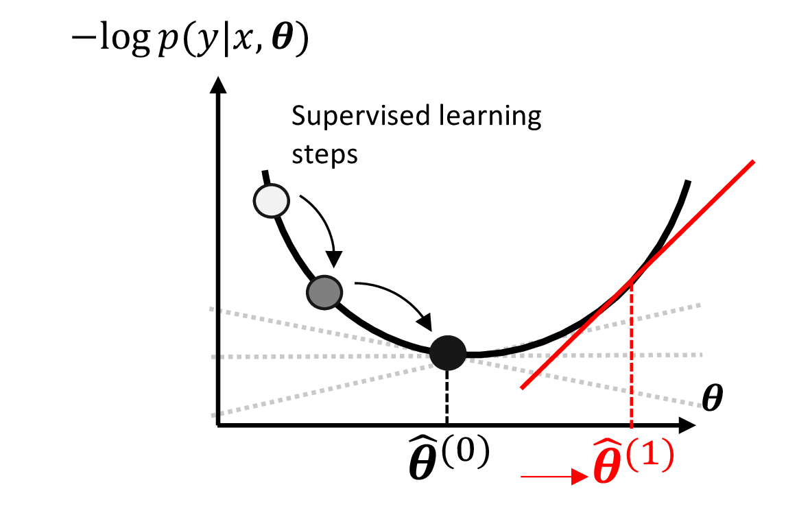
Let \(\{(\mathbf{x}_i, y_i)\}_{i=1}^{n}\) denote a training dataset of \(n\) independent observations, where \(\mathbf{x}_i \in \mathbb{R}^p\) is the covariate vector and \(y_i \in \mathbb{R}\) (or a categorical label) is the response for the \(i\)-th observation. We assume the data are generated from a parametric conditional distribution \(P(Y \mid \mathbf{X};\, \boldsymbol{\theta})\), indexed by a parameter vector \(\boldsymbol{\theta} \in \mathbb{R}^q\). The supervised learning model, parameterized by \(\hat{\boldsymbol{\theta}}^{(0)}\), is fit by maximizing the log-likelihood over the training data (assumed in-control, without drift), yielding the maximum likelihood estimate (MLE): \[\hat{\boldsymbol{\theta}}^{(0)} \;=\; \arg\max_{\boldsymbol{\theta}} \;\frac{1}{n}\sum_{i=1}^{n} \log P\!\left(y_i \mid \mathbf{x}_i;\, \boldsymbol{\theta}\right). \label{eq:mle}\tag{7}\] The Fisher score vector (hereafter, the score vector) for a single observation \((\mathbf{x}_t, y_t)\) evaluated at the fitted parameters \(\hat{\boldsymbol{\theta}}^{(0)}\) is defined as the gradient of the log-likelihood with respect to \(\boldsymbol{\theta}\): \[\mathbf{s}_t \;:=\; \mathbf{s}\!\left(\hat{\boldsymbol{\theta}}^{(0)};\, (\mathbf{x}_t, y_t)\right) \;=\; \nabla_{\!\boldsymbol{\theta}}\, \log P\!\left(y_t \mid \mathbf{x}_t;\, \boldsymbol{\theta}\right) \Big|_{\boldsymbol{\theta} = \hat{\boldsymbol{\theta}}^{(0)}}, \label{eq:score}\tag{8}\] where \(\nabla_{\!\boldsymbol{\theta}}\) denotes the gradient operator with respect to \(\boldsymbol{\theta}\). The score vector enjoys a key zero-mean property that forms the theoretical foundation of the detection framework. Under the assumption that the model is correctly specified and the true parameter vector is \(\boldsymbol{\theta}^{(0)}\), MLE theory gives \[\mathbb{E}_{\boldsymbol{\theta}^{(0)}}\!\left[ \mathbf{s}\!\left(\boldsymbol{\theta}^{(0)};\,(\mathbf{X},Y)\right) \mid \mathbf{X} \right] = \mathbf{0}. \label{eq:zero95mean}\tag{9}\] Equivalently, at the MLE, the average score vector over the training data is identically zero by the first-order optimality condition, as shown in Figure 6: \[\frac{1}{n}\sum_{i=1}^{n} \mathbf{s}\!\left(\hat{\boldsymbol{\theta}}^{(0)};\,(\mathbf{x}_i, y_i)\right) = \mathbf{0}. \label{eq:empirical95zero}\tag{10}\] This property holds regardless of whether the assumed model structure is correctly specified, because it follows directly from the definition of the MLE as a stationary point of the training log-likelihood. Now suppose that after the model is deployed, the true conditional distribution drifts from \(P(Y \mid \mathbf{X};\, \boldsymbol{\theta}^{(0)})\) to a new distribution characterized by \(\boldsymbol{\theta}^{(1)} \neq \boldsymbol{\theta}^{(0)}\). Under this new regime, the expected score vector, still evaluated at the original parameters \(\hat{\boldsymbol{\theta}}^{(0)}\), becomes \[\mathbb{E}_{\boldsymbol{\theta}^{(1)}}\!\left[ \mathbf{s}\!\left(\boldsymbol{\theta}^{(0)};\,(\mathbf{X},Y)\right) \mid \mathbf{X} \right] \;\neq\; \mathbf{0}, \label{eq:nonzero95drift}\tag{11}\] for any \(\boldsymbol{\theta}^{(1)} \neq \boldsymbol{\theta}^{(0)}\) under mild identifiability conditions. Equations 9 –11 together imply that concept drift has occurred if and only if the mean of the score vector departs from zero [62]. This equivalence motivates monitoring the empirical mean of \(\mathbf{s}_t\) over time as the basis for a drift-detection procedure. For models fitted via gradient descent, NN models in particular, the score vectors are obtained via backpropagation, incurring minimal additional computational cost.
3.3.2 Drift Detection Framework↩︎
3.3.2.1 Phase I: Retrospective Analysis and Control Limit Estimation.
Collect a batch of chronologically ordered observations \(\mathcal{D} = \{(\mathbf{x}_i, y_i)\}_{i=1}^{m}\) from the historical record and partition it into two subsets: \(\mathcal{D}_1 = \{(\mathbf{x}_i, y_i)\}_{i=1}^{m_1}\) for estimating the distribution of the score vector, and \(\mathcal{D}_2 = \{(\mathbf{x}_i, y_i)\}_{i=m_1+1}^{m}\) for estimating the control limit. With a pre-trained parametric supervised model fit offline and its MLE \(\hat{\boldsymbol{\theta}}^{(0)} \in \mathbb{R}^q\) (Equation 7 ), the score vector \(\mathbf{s}_i\) is then computed for each \((\mathbf{x}_i, y_i) \in \mathcal{D}_1\) at the fixed \(\hat{\boldsymbol{\theta}}^{(0)}\) (Equation 8 ), and further used to compute the mean of the score vector \(\bar{\mathbf{s}}\) and the covariance of the score vector \(\widehat{\boldsymbol{\Sigma}}\).
Note that fitting \(\bar{\mathbf{s}}\) and \(\widehat{\boldsymbol{\Sigma}}\) on held-out data different from the training set avoids the bias of reusing \(\mathcal{D}_1\), so the scores reflect the model’s sensitivity to new data rather than to the training set. Therefore, with batch \(\mathcal{D}_2\) that is independent from \(\mathcal{D}_1\), the score sequence using \(\mathcal{D}_2\) as the streaming data at the with \(\hat{\boldsymbol{\theta}}^{(0)}\) is smoothed using the Multivariate EWMA (MEWMA) recursion [93], \[\mathbf{z}_t \;=\; \lambda\, \mathbf{s}_t \;+\; (1 - \lambda)\,\mathbf{z}_{t-1}, \qquad t = 1, 2, \ldots,\, m-m_1, \label{eq:mewma}\tag{12}\] where \(\lambda \in (0,1]\) controls the effective memory (\(\approx 1/\lambda\) observations) and \(\mathbf{z}_0\) is the \(\bar{\mathbf{{s}}}\). To reduce the \(q\)-dimensional \(\mathbf{z}_t\) to a scalar monitoring statistic, the Hotelling \(T^2\) statistic, i.e.the Mahalanobis distance of \(\mathbf{z}_t\) from the reference mean \(\bar{\mathbf{s}}\), is used, \[T_t^2 \;=\; \left(\mathbf{z}_t - \bar{\mathbf{s}}\right)^{\!\top} \widehat{\boldsymbol{\Sigma}}^{-1} \left(\mathbf{z}_t - \bar{\mathbf{s}}\right). \label{eq:t2}\tag{13}\] When \(\widehat{\boldsymbol{\Sigma}}\) is singular or ill-conditioned, a nugget regularization \(\widehat{\boldsymbol{\Sigma}} \leftarrow \widehat{\boldsymbol{\Sigma}} + \delta \mathbf{I}\) is applied, with \(\delta > 0\) the smallest value bringing the condition number below a prescribed threshold.
The upper control limit (UCL) is set as the \((1-\alpha)\) empirical quantile of \(\{T_t^2\}\) over \(\mathcal{D}_2\), where \(\alpha\) is the nominal false-alarm rate. This nonparametric limit requires no distributional assumption and reflects the variability of the reference data directly; estimating it on a batch separate from model fitting and scoring prevents the underestimated variability and inflated false-alarm rates that double use would induce.
3.3.2.2 Phase II: Prospective Online Monitoring.
As each time step as new observation arrives, the score \(\mathbf{s}_t\) is computed at the estimate \(\hat{\boldsymbol{\theta}}^{(0)}\), the MEWMA recursion 12 and statistic 13 are continued, and at the hypothesis \[\begin{align} H_0 &: \mathbb{E}\!\left[\mathbf{s}\!\left(\hat{\boldsymbol{\theta}}^{(0)};\,(X,Y)\right)\right] = \mathbf{0}\quad\text{(no drift)},\\ H_1 &: \mathbb{E}\!\left[\mathbf{s}\!\left(\hat{\boldsymbol{\theta}}^{(0)};\,(X,Y)\right)\right] \neq \mathbf{0}\quad\text{(drift present)} \label{eq:hypothesis} \end{align}\tag{14}\] is evaluated by computing the \(T^2\) statistics on new observations. A drift alarm is raised when \(T_t^2>\mathrm{UCL}\), upon which monitoring pauses and the fine-tuning procedure of Section 3.4 begins.
3.3.3 Drift Detection for Neural Networks↩︎
From a statistical perspective, monitoring the score vector of the last layer is a sufficient and efficient approach for detecting distributional changes that affect model outputs, suggested by [62]. When focusing on the last layer, the score captures deviations in the conditional distribution \(p(y\mid z)\), where \(z\) denotes the learned latent representation from preceding layers. For many engineering applications, the drift of interest is precisely a change in this conditional relationship, rather than a complete restructuring of the feature extractor.
Detecting drift only on the last-layer parameters also improves statistical efficiency since estimating the covariance of the full score vector in high dimensions is often ill-conditioned and data-intensive, reducing detection power and increasing memory usage. In contrast, the lower-dimensional last-layer score enables more stable covariance estimation and more reliable test statistics. This yields a favorable trade-off in detection efficiency while ensuring robust inference in streaming, data-limited settings.
3.3.4 Online Implementation of Score-Based Drift Detection for Quantile Prediction↩︎
The detection framework reviewed above presumes a likelihood-based model and an offline Phase I calibration. Integrating it into an operating Digital Twin whose surrogate is trained with quantile losses requires the following adaptations. We treat the quantile loss as a pseudo log-likelihood to construct the score vector. Although the quantile loss does not correspond to a true likelihood, it provides a consistent gradient signal with respect to the model parameters. Its gradient can therefore be interpreted as a pseudo score function that reflects the sensitivity of the model to distributional changes. This formulation enables the simultaneous monitoring of multi-step, multi-level quantile predictions within a unified framework, without requiring separate detectors for different prediction horizons or quantile levels.
The score vector, obtained via backpropagation, drives Phase II monitoring (Section 3.3.2.2); on detection, the framework adapts (Section 3.4.2) and validates (Section 3.5) the model, after which the detector must be reset. Unlike the offline Phase I, online re-initialization must be computationally and data efficient, since operation continues in real time.
A primary online bottleneck is inverting the covariance \(\hat{\boldsymbol{\Sigma}}^{-1}\in\mathbb{R}^{\tilde{q}^2\times \tilde{q}^2}\) (\(\tilde{q}\) the last-layer output dimension),
costing \(\mathcal{O}(\tilde{q}^6)\) and being statistically unreliable when estimated from limited data. We therefore conducted an empirical study on approximating \(\hat{\boldsymbol{\Sigma}}\) by its diagonal (\(\mathcal{O}(\tilde{q}^2)\) inversion, more stable estimates) and also consider Kronecker-Factored Approximate Curvature (K-FAC) [94]. Details of this approximation and an empirical comparison of the covariance strategies are provided in the Supplementary
Information (SI). Here, we compared three strategies for the covariance term \(\hat{\boldsymbol{\Sigma}}^{-1}\) in the Hotelling \(T^2\) statistic on a nonlinear scalar-regression benchmark
with heteroscedastic, asymmetric noise: exact full-covariance inversion (FULL), a diagonal approximation (DIAG), and K-FAC (KFAC). Across both a mean-shift drift and a variance-only drift, DIAG
consistently achieved the shortest detection delay and the lowest false-alarm rate, trading a small covariance bias for a large reduction in estimation variance, whereas KFAC offered no advantage over FULL. We therefore adopt
DIAG for computing \(\hat{\boldsymbol{\Sigma}}^{-1}\) throughout this work. The full experimental setup, figures, and analysis are provided in the SI.
Estimating the UCL online is a second bottleneck for the online implementation of Phase II. Formally, the empirical-quantile approach requires \(\sim 1/\alpha\) samples (e.g.\(10^4\) for \(\alpha=10^{-4}\)) to estimate the UCL, making it impractical to reset the drift detector during operation. We instead fit the upper tail of the \(T^2\) distribution, assuming \(T^2\) is stationary after adaptation and approximating it by a scaled non-central \(\chi^2\) via moment matching. Although the Hotelling \(T^2\) statistic follows an \(F\) distribution under certain assumptions [95], this no longer holds here, as the MEWMA induces temporal dependence (see SI). Because tail fitting from limited data is sensitive to outliers, we additionally bootstrap the \(T^2\) values to obtain multiple UCL estimates, whose median is used as the drift-detection threshold.
These modifications enable an efficient online Phase I re-initialization that requires relatively small batches and avoids full covariance inversion, making score-based detection feasible in real-time applications.
3.4 How to Update the Digital Twin? – Parameter-Efficient Model Adaptation↩︎
Once drift is detected, the second module updates the surrogate from a limited buffer of streaming data. As discussed in the Introduction, the update mechanism must supply enough plasticity to capture the new regime while preserving the pretrained structure that remains valid, and must do so from few samples without destabilizing ongoing operation. We address the first requirement with LoRA, reviewed in Section 3.4.1, and the second with the batch-wise fine-tuning procedure of Section 3.4.2.
3.4.1 Low-Rank Adaptation↩︎
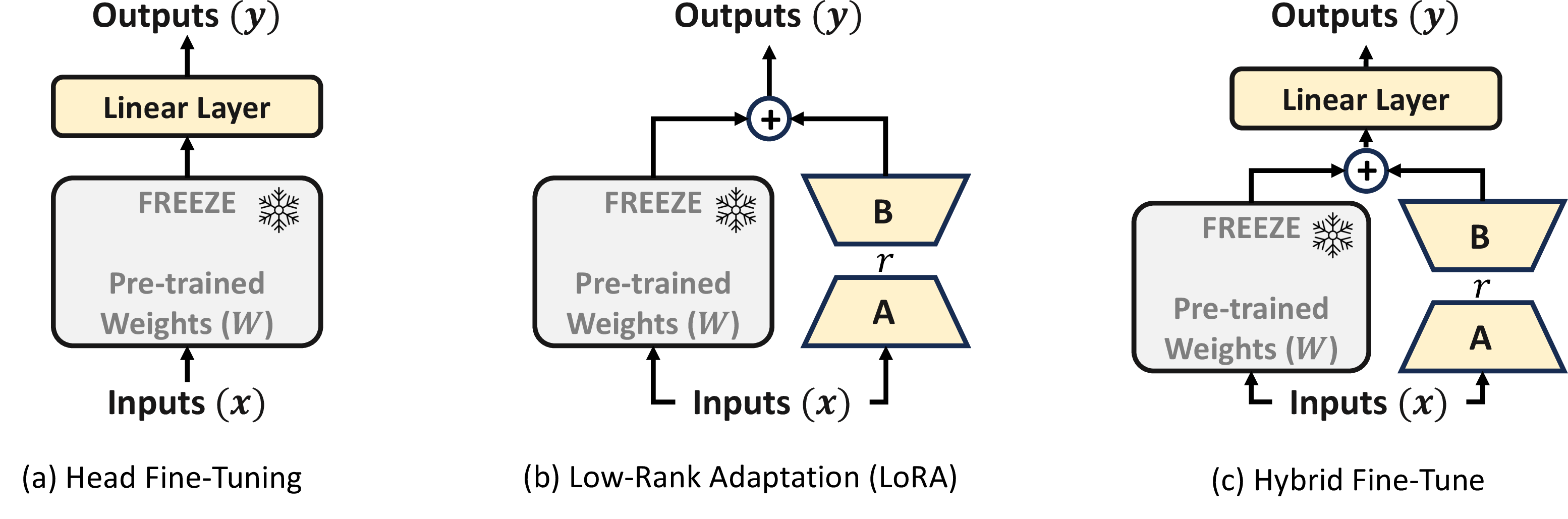
Low-rank adaptation (LoRA) [69], a widely used PEFT method for large language models, constrains task-specific adaptation to a low-rank subspace of the pretrained weights, as illustrated in Figure 7 (b). By restricting fine-tuning to this low-dimensional subspace, LoRA improves data and parameter efficiency while providing sufficient plasticity for model adaptation, with the pretrained network retained to balance the model’s stability. For a linear layer \(y=\mathbf{W}x\) with \(\mathbf{W}\in\mathbb{R}^{d\times k}\), LoRA freezes \(\mathbf{W}\) and learns an additive low-rank update \[\mathbf{W}' = \mathbf{W} + \Delta \mathbf{W}, \quad \Delta \mathbf{W} = \mathbf{B A},\] with \(\mathbf{A}\in\mathbb{R}^{r\times k}\) and \(\mathbf{B}\in\mathbb{R}^{d\times r}\), reducing the number of trainable parameters from \(dk\) to \(r(d+k)\) for \(r \ll \min(d,k)\). Initializing \(\mathbf{B}=\mathbf{0}\) makes \(\Delta \mathbf{W}=\mathbf{0}\) at the start, so the model exactly reproduces the pretrained mapping before adaptation and departs from it only as evidence accumulates from the new regime.
The low-rank constraint is not merely a computational convenience but a structural hypothesis about how adaptation manifests, one that is well matched to concept drift in engineered systems. Empirical studies of over-parameterized networks show that fine-tuning updates possess low intrinsic dimensionality, i.e.the weight correction required to specialize a pretrained model resides in a subspace of dimension far smaller than the total number of parameters [69], [96]. This hypothesis is plausible for the drift scenarios considered here, where physical drift typically arises from parameter variation, wear, or environmental change that perturbs the governing dynamics smoothly rather than restructuring them entirely. The latent representations learned by the pretrained surrogate, encoding temporal features and input–response couplings, therefore remain largely valid under drift, and adaptation reduces to reweighting how these features are combined, a correction naturally expressible as a low-rank perturbation of the weight matrices. This stands in contrast to head fine-tuning, which can only rescale and recombine the fixed output features and thus fails when drift alters the internal dynamics that generate those features, and to full fine-tuning, whose unconstrained updates can distort the shared representation from few noisy samples.
From an estimation-theoretic perspective, restricting the update to \(r(d+k)\) degrees of freedom directly addresses the low-data pathology of streaming adaptation. With a buffer of only \(N_B\) samples, estimating a full-rank correction is severely underdetermined and highly sensitive to measurement noise, whereas the low-rank parameterization shrinks the effective hypothesis space, reducing estimation variance and acting as an implicit regularizer that complements the explicit weight penalty used during fine-tuning. The rank \(r\) moreover serves as an interpretable design knob for the stability–plasticity trade-off central to continual learning, where small \(r\) yields conservative, well-conditioned updates suitable for mild drift, while larger \(r\) grants additional plasticity for severe regime changes. However, the selection of the rank highly depends on the available buffer size and fine-tuning requirements, depending on different applications.
LoRA also offers deployment properties that align closely with the architecture of the proposed framework. Because the update is additive to each layer without changing the model’s structure, the adapted surrogate incurs negligible inference latency since the rank \(r \ll d\), and one not shared by adapter-style methods that insert serial layers into the forward pass [82]. Moreover, the modularity of low-rank updates suggests a natural extension in which validated \(\{\mathbf{B}_j\mathbf{A}_j\}\) pairs are archived as a library of regime-specific corrections, enabling rapid re-deployment upon recurrence of previously encountered operating conditions rather than re-adaptation from scratch. This direction is left to future work. Because \(\mathbf{W}\) remains frozen throughout, the pretrained backbone is preserved intact, mitigating catastrophic forgetting by construction rather than through auxiliary replay or regularization losses. To benchmark against existing methods, we also implement head fine-tuning (Figure 7 (a)) and a hybrid method that combines head fine-tuning with LoRA (Figure 7 (c)).
3.4.2 Batch-Wise Model Adaptation↩︎
Once drift is detected, the framework transitions to the model-adaptation stage. Prior to data collection, the system is operated over a full prediction horizon \(N\) to ensure that all samples used for fine-tuning are obtained directly from the physical system rather than from model-generated predictions [47]. This step is essential to prevent bias introduced by previously drifted models. Following this initialization, a data batch of size \(N_B\) is collected. Adopting a batch-based strategy improves the robustness and generalizability of the fine-tuning process while reducing the risk of overfitting to transient disturbances or anomalous observations, which is equivalent to the stochastic weight averaging (SWA) concept of adapting parameters over a short horizon at every time step [47], [97], [98]. Such a design is also consistent with common practice in model-based reinforcement learning [99].
Once the data buffer is full, the collected dataset is partitioned into training and validation subsets using a 9:1 ratio. Rather than performing a contiguous split at a specific time index, validation samples are periodically extracted from the streaming data every 10 steps, with the remaining samples assigned to the training set. This interleaved splitting strategy ensures that both subsets remain representative of the same underlying data distribution, which is particularly important in non-stationary environments [84]. As a result, the validation process more reliably reflects the model’s generalization performance under evolving system dynamics.
With the dataset prepared, the idle model is fine-tuned using the training set. Optimization is carried out with the Adam optimizer for 100 epochs using mini-batch updates. To mitigate overfitting, a regularization term is incorporated into
the loss function, and the validation loss is monitored at each epoch; the model achieving the lowest validation loss is selected as the updated model. Within this framework, the three fine-tuning strategies introduced in Section 3.4.1 are evaluated.
Finally, the proposed adaptation strategy imposes minimal computational overhead for real-time deployment. Although each fine-tuning cycle uses larger batches and more epochs than per-step updates, it runs entirely on the idle model and does not interfere with ongoing operation. Moreover, because adaptation is followed by a validation stage that itself requires collecting a batch of streaming data, the fine-tuning cost is effectively hidden when executed in parallel with validation-batch collection. The framework also permits fine-tuning to run on hardware separate from the real-time controller, avoiding any additional burden or latency in time-critical optimization.
3.5 Is the Update Successful? – Model Validation↩︎
Once the idle model has been fine-tuned, the framework proceeds to the model-validation stage, where its predictive performance is formally assessed to determine whether it should replace the live model. Specifically, we compare the supervised-learning loss produced by the live and idle models on a validation dataset. This validation set is strictly held out from the fine-tuning process to prevent data leakage and ensure an unbiased evaluation of generalization performance. An additional batch of data of size \(N_V\) is therefore collected after the adaptation stage to construct the validation set.
Given the validation data, the live and idle models receive the same validation input, and their predictions are compared against the ground truth using the quantile loss. This yields two empirical distributions of loss values. The validation task is then formulated as a hypothesis test of whether the idle model achieves a statistically significant reduction in loss relative to the live model. As the loss distributions are not guaranteed to be Gaussian, parametric tests on the mean are inappropriate. Instead, we adopt the Mann–Whitney \(U\) test [100], a nonparametric rank-based test that evaluates stochastic dominance without distributional assumptions (See SI for details on Mann-Whitney \(U\) test). The one-sided hypothesis test is defined as \[\begin{align} H_0 &: P(\mathcal{L}_\text{idle} > \mathcal{L}_\text{live}) \geq 0.5, \\ H_1 &: P(\mathcal{L}_\text{idle} > \mathcal{L}_\text{live}) < 0.5. \end{align}\] Rejection of \(H_0\) indicates that the idle model is statistically more likely to produce lower loss than the live model, implying improved predictive performance. In this case, the idle model replaces the live model for subsequent decision-making. Otherwise, the evidence is insufficient to justify replacement, and the framework returns to the adaptation stage, where the idle model continues to be refined as additional data become available. The flowchart of the model validation stage is illustrated in Figure 8. Due to the limited number of validation set, the significance level is set to 0.2 in this work.
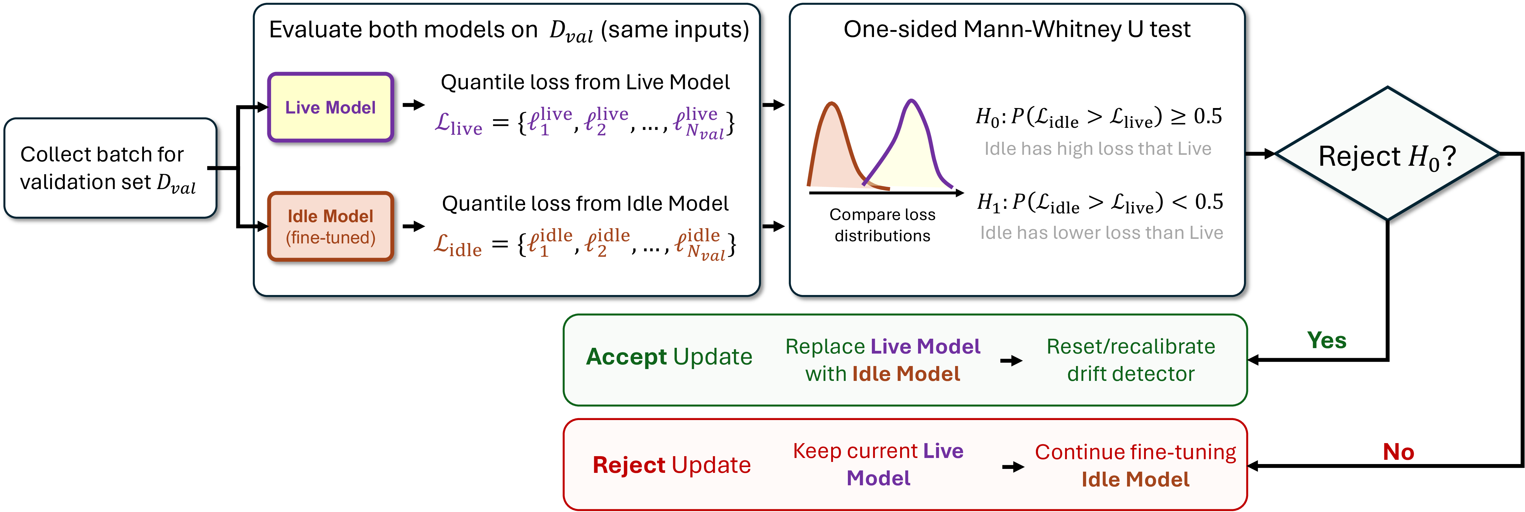
Ideally, one would compare the magnitudes of the score vectors or the Hotelling \(T^2\) statistic rather than the loss values. However, comparing the Hotelling \(T^2\) requires re-estimation of both \(\bar{\mathbf{s}}\) and \(\hat{\Sigma}^{-1}\), which is not sufficiently data-efficient in an online setting. Consequently, as a pragmatic compromise, we adopt direct comparison of loss values for online validation.
Following model replacement, the framework re-enters Phase I to reinitialize the drift detector using the updated model, as described in Section 3.3.4. Collectively, the integration of drift detection, model adaptation, and statistical validation establishes an autonomous framework that enables the Digital Twin to continuously adapt to evolving operating conditions throughout its life cycle. While the proposed batch-wise adaptation strategy may exhibit slower responsiveness than step-wise updates, it provides statistically grounded guarantees on model improvement, ensuring that updates preserve generalization performance rather than overfitting to transient data.
We argue that the model-validation stage is essential even when validation loss is monitored during fine-tuning. This design follows the standard training–validation–testing paradigm in supervised learning, where the testing stage evaluates a model’s ability to generalize to unseen data. Such evaluation is essential for Digital Twins operating under non-stationary conditions, where the fine-tuning and validation datasets are sampled from the same distribution, whereas the input distribution, \(p(x)\), of future streaming data may drift from this distribution even when the underlying concept, \(p(y \mid x)\), remains unchanged. Consequently, an additional validation stage on unseen data provides a more reliable assessment of generalization and can reveal overfitting not apparent from the fine-tuning loss alone. For instance, a monotonically decreasing validation loss during fine-tuning does not guarantee deployability; failure to reject \(H_0\) indicates that there is insufficient evidence of improvement of the updated model on newly arriving data and therefore should not replace the live model. In such cases, a more appropriate strategy is to continue fine-tuning as additional streaming data becomes available, leveraging the adaptability of the pretrained network. Alternative approaches, such as adaptive regularization schemes or improved data-buffer strategies to enhance generalization, are promising directions but are beyond the scope of this work.
4 Illustrative Example↩︎
In this section, the illustrative example introduced in [6] is used to walk through the proposed method and to benchmark against existing fine-tuning approaches. A discrete-time linear system with states \(\mathbf{x}=[x_1,x_2]^\top\) is considered for demonstration. Initially, the system is subject to additive stochastic disturbance on \(x_2\), where \(\epsilon_k \sim \mathcal{N}(0, 1^2)\), described by \[\begin{align} \mathbf{x}_{k+1} &= \mathbf{A}\mathbf{x}_k + \mathbf{B}u_k + \mathbf{w}_k\\ &= \begin{bmatrix} 0.3 & 0.1 \\ 0.1 & 0.2 \end{bmatrix} \mathbf{x}_k + \begin{bmatrix} 0.5 \\ 1 \end{bmatrix} u_k + \begin{bmatrix} 0\\0.1 \end{bmatrix} \epsilon_k \\ &= F_w(\mathbf{x}_k, u_k, \mathbf{w}_k),\\ \mathbf{y}_{k+1} & = \mathbf{x}_{k+1} \label{eq:toy95problem95sys} \end{align}\tag{15}\] where the disturbance follows a Gaussian distribution due to the linear transformation of \(\epsilon_k\).
4.1 Building the Virtual Twin: Surrogate Modeling↩︎
To construct training data for system identification with TiDE, an input sequence \(\mathbf{D}_u = \{u_0, \ldots, u_{n-1}\}\) is generated, where \(u_k \in [-5,5]\) is uniformly sampled and \(n = 422{,}000\). Starting from the initial condition \(\mathbf{x}_0 = [0,0]^T\), the corresponding state trajectory \(\mathbf{D}_x = \{\mathbf{x}_1, \ldots, \mathbf{x}_n\}\) is obtained by forward simulation. The detailed training configuration is summarized in Table 1.
The resulting sequences are segmented using a sliding window of length \(w + N\), where the window size is \(w = 10\) and the prediction horizon is \(N = 10\). For the \(l\)th segment, define \[\begin{align} \mathbf{D}_{u,l} &= \{u_l, \ldots, u_{l+w+N-1}\}, \\ \mathbf{D}_{x,l} &= \{\mathbf{x}_{l+1}, \ldots, \mathbf{x}_{l+w+N}\}. \end{align}\] Each segment is then decomposed into past and future components: \[\begin{align} \mathbf{x}^p_l &= [\mathbf{x}_{l+1}, \ldots, \mathbf{x}_{l+w}], \quad \mathbf{x}^f_l = [\mathbf{x}_{l+w+1}, \ldots, \mathbf{x}_{l+w+N}], \\ \mathbf{u}^p_l &= [u_l, \ldots, u_{l+w-1}], \quad \mathbf{u}^f_l = [u_{l+w}, \ldots, u_{l+w+N-1}], \end{align}\] where the superscripts \(p\) and \(f\) denote the past and future components, respectively. The tuple \((\mathbf{x}^p_l, \mathbf{u}^p_l, \mathbf{u}^p_l)\) serves as input and \(\mathbf{x}^f_l\) as the prediction target.
All segments are randomly partitioned into training, validation, and test sets with a ratio of 8:1:1. Following Eq. (5 ), the TiDE model is trained via supervised learning using the quantile loss: \[\begin{align} \min_{\boldsymbol{\phi}} \quad & L_Q(\mathbf{x}^f, \hat{\mathbf{x}}^f), \\ \text{s.t.} \quad & \hat{\mathbf{x}}^f = \text{TiDE}(\mathbf{x}^p, \mathbf{u}^p, \mathbf{u}^f \mid \boldsymbol{\phi}). \end{align}\]
As the focus is the adaptive framework rather than surrogate accuracy, we report only that the trained TiDE attains \(\approx 5\%\) MAPE and \(\approx 0.04\) NRMSE on both states (see [6] for full validation), which is sufficient for the following tasks.
| Details for TiDE model setup | ||||||
|---|---|---|---|---|---|---|
| # encoder layers | # decoder_layers | decoder output dim. | hidden size | decoder hidden size | dropout rate | layer normalization |
| 1 | 1 | 16 | 128 | 32 | 0.2 | True |
| Details for TiDE model training | ||||||
| learning rate | regularization | step_size | rate decay | # epoch | batch size | shuffle data |
| 0.001 | 0.002 | 10 | 0.95 | 1500 | 64 | True |
4.2 Uncertainty-Aware Decision-Making through Robust Model Predictive Control↩︎
The physical system and its virtual twin interact through a robust MPC: at each step, measurements from the physical system update the state for predicting quantiles through TiDE, which is then used in robust MPC to build safety margins for explicit constraint handling under uncertainty, and the optimal input is applied to the physical system.
The objective of this example is to regulate the state \(x_1\) to track a reference trajectory while ensuring that \(x_1\), \(x_2\), and the control input \(u\) remain within admissible bounds in the presence of unbounded disturbances. The multi-step robust MPC formulation, leveraging quantile predictions from TiDE, is given by \[\label{eq:MPC95toy} \begin{align} \min_{\mathbf{v}} \quad & J(\mathbf{v},\tilde{\hat{\mathbf{x}}},\mathbf{r}) = \sum_{i=0}^{N-1} \|\tilde{\hat{x}}_{1,k+i+1} - r_{k+i+1}\|_{\mathbf{Q}}^2 + \|v_{k+i}\|_{\mathbf{R}}^2 \\ \text{s.t.} \quad & \hat{\mathbf{x}}_{k+1}^f = [\bar{\hat{\mathbf{x}}}_{k+1}^{f}, \tilde{\hat{\mathbf{x}}}_{k+1}^{f}, \underline{\hat{\mathbf{x}}}_{k+1}^{f}]^T = \text{TiDE}(\mathbf{x}_{k}^p, \mathbf{u}_{k}^p, \mathbf{v}), \\ & \mathbf{v} = [v_k,\ldots,v_{k+N-1}], \\ & \text{Pr}\left(\hat{x}_{1,k+i} \geq -2 \right) \geq 0.95, \quad \forall i \in \mathbb{N}_{[1,N]}, \\ & \text{Pr}\left(\hat{x}_{1,k+i} \leq 2.5 \right) \geq 0.95, \quad \forall i \in \mathbb{N}_{[1,N]}, \\ & \text{Pr}\left(\hat{x}_{2,k+i} \geq -3.5 \right) \geq 0.95, \quad \forall i \in \mathbb{N}_{[1,N]}, \\ & \text{Pr}\left(\hat{x}_{2,k+i} \leq 3.5 \right) \geq 0.95, \quad \forall i \in \mathbb{N}_{[1,N]}, \\ & v_{k+i} \in \mathbb{U} \ominus \mathbf{K}\mathbb{Z}_{k+i}, \quad \forall i \in \mathbb{N}_{[0,N-1]}, \\ & u_k = \pi(v_k) = v_k + \mathbf{K}\mathbf{e}_k, \\ & \mathbf{u}_{k}^p = [u_{k-w},...,u_{k-1}]. \end{align}\tag{16}\]
The weighting matrices are chosen as \(\mathbf{Q} = \mathbf{I}\) and \(\mathbf{R} = \mathbf{I}\). The admissible input set is \(\mathbb{U} \in [-5,5]\), adaptively tightened based on the prediction-error bound \(\mathbb{Z}\). The feedback gain is selected as \(\mathbf{K} = [-0.0621, -0.2027]\). Since the predicted upper and lower quantiles inherently capture the probabilistic bounds on the states, the chance constraints in (16 ) can be equivalently reformulated as deterministic constraints: \[\begin{align} & \bar{\hat{x}}_{1,k+i} \leq 2.5, \quad \underline{\hat{x}}_{1,k+i} \geq -2, \\ & \bar{\hat{x}}_{2,k+i} \leq 3.5, \quad \underline{\hat{x}}_{2,k+i} \geq -3.5. \end{align}\]
4.3 Phase I: Drift Detector Setup↩︎
To enable online score-based detection, the pretrained TiDE (187,278 parameters) is frozen, LoRA layers are added to each layer, and an additional linear output layer producing the score vector is appended. The score is defined as the gradient of the loss with respect to this final linear layer (3,600 parameters), so the LoRA layers (2,670 parameters) are also frozen during detection and are unfrozen only at the model-adaptation stage, giving 6,270 tunable parameters, which is just \(3.3\%\) of the full pretrained model under the hybrid strategy.
To calibrate the drift detector in Phase I, 700 undrifted steps are first collected. The first 200 estimate the score mean \(\bar{\mathbf{s}}\) and covariance \(\hat{\Sigma}\) (with \(\hat{\Sigma}^{-1}\) from diagonal inversion), and the remaining 500 give the sequential MEWMA \(T^2\) statistic (Eqs. 12 –13 , \(\lambda=0.05\)). Its empirical distribution is fit by a scaled noncentral \(\chi^2\) via bootstrapping, and the threshold \(h\) is set at significance \(\alpha=10^{-5}\).
Note that although TiDE is trained with a multi-step-ahead quantile loss, the score vector is computed from the one-step-ahead quantile loss. This choice enables earlier drift detection, as one-step-ahead predictions respond immediately to changes, whereas multi-step-ahead predictions may not reflect the drift until several time steps later. From a dynamical-systems perspective, inaccurate one-step-ahead predictions typically propagate to future predictions through error accumulation; monitoring the one-step-ahead prediction error therefore provides a more direct and sensitive indicator of model drift.

Figure 9 illustrates the trajectory of the multi-step RMPC under in-control conditions. The proposed RMPC framework effectively trades off reference-tracking performance to maintain constraint satisfaction in the presence of fluctuations, enabled by the safety margins provided by the learned quantiles.
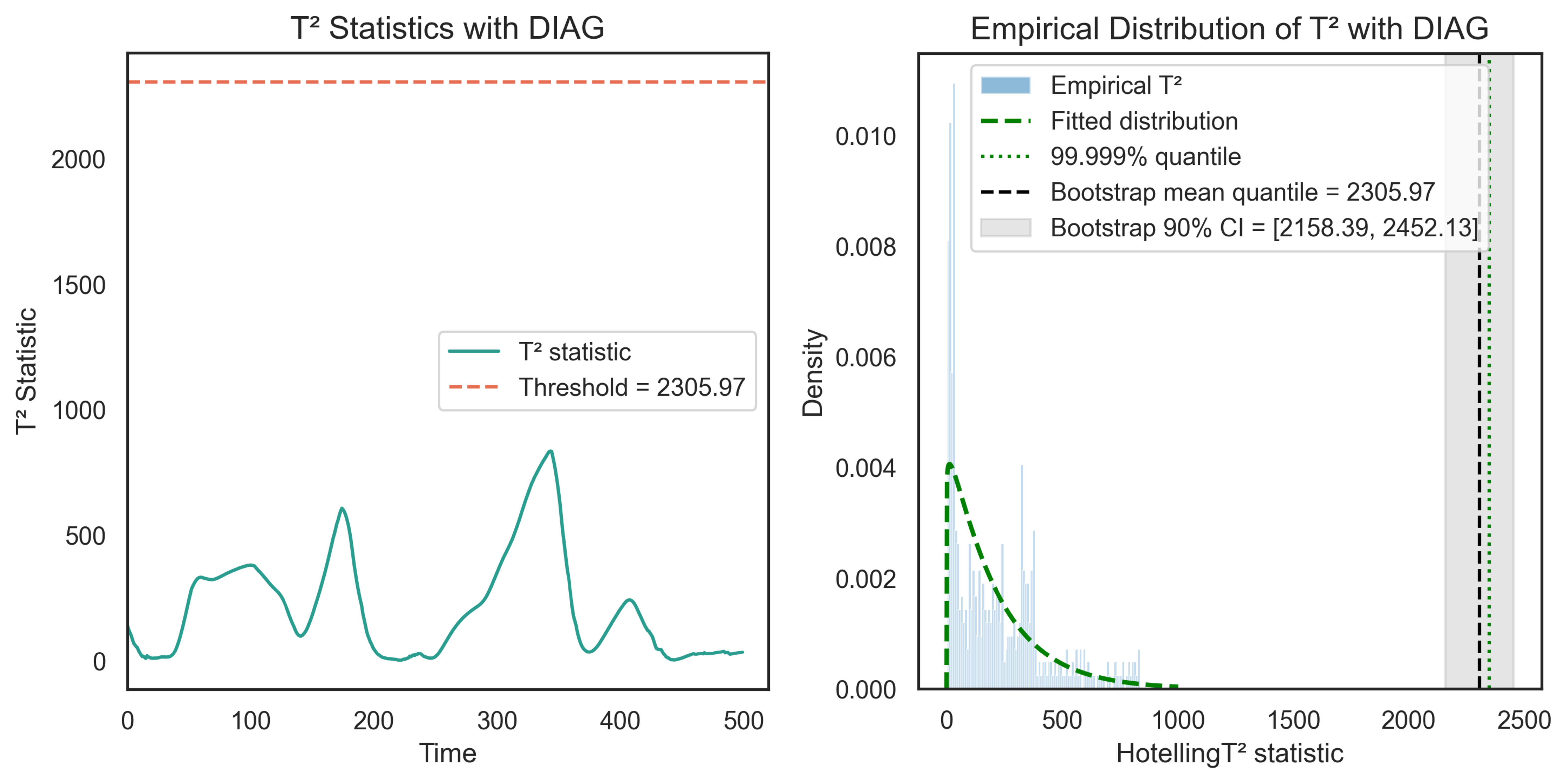
The corresponding \(T^2\) trajectory and its histogram are presented in Figures 10 (a) and 10 (b), respectively. In Figure 10 (a), the horizontal dashed line represents the detection threshold. Under stationary conditions, the \(T^2\) statistic fluctuates around a stable level and remains below the threshold. Figure 10 (b) further shows that the empirical distribution of \(T^2\) is well approximated by the fitted scaled noncentral \(\chi^2\) distribution.
4.4 Phase II: Online Drift Detection, Adaptation, and Validation↩︎
In Phase II the tracking task runs for 3,000 steps with abrupt changes at \(k=200\) and \(k=1500\). At \(k=200\) the system enters concept \(P_1(y\mid x)\), injecting three uncertainties: nonlinear terms for previously unmodeled dynamics, modified \(\mathbf{A},\mathbf{B}\) for changed intrinsic dynamics, and a noise reduction \(\mathcal{N}(0,0.1^2)\!\to\!\mathcal{N}(0,0)\) that probes the adaptability of the learned quantiles. The resulting state evolution under concept \(P_1(y \mid x)\) is given by \[\begin{align} \mathbf{x}_{k+1} &= \begin{bmatrix} 0.5 & 0.04\\ 0.2 & 0.2 \end{bmatrix}\mathbf{x}_k + \begin{bmatrix} 0.5\\ 1 \end{bmatrix}u_k + 0.3 \begin{bmatrix} 1 & 0\\ 0 & 1 \end{bmatrix} \tanh(\mathbf{x}_k) + 0.1 \begin{bmatrix} 1\\ 1 \end{bmatrix} \tanh(u_k) + \begin{bmatrix} 0\\ 0 \end{bmatrix}\epsilon_k, \label{eq:toy95nonlinear95matrix95p1} \end{align}\tag{17}\] where \(\epsilon_k \sim \mathcal{N}(0, 1)\).
At \(k = 1500\), the system transitions to another regime, concept \(P_2(y \mid x)\). Here the disturbance is allowed to affect both state variables, representing an increase in aleatoric uncertainty. In addition, the system matrices are altered again, introducing further epistemic uncertainty. The resulting system under concept \(P_2(y \mid x)\) is \[\begin{align} \mathbf{x}_{k+1} &= \begin{bmatrix} 0.6 & 0.25\\ 0.2 & 0.4 \end{bmatrix}\mathbf{x}_k + \begin{bmatrix} 0.5\\ 1 \end{bmatrix}u_k + 0.3 \begin{bmatrix} 1 & 0\\ 0 & 1 \end{bmatrix} \tanh(\mathbf{x}_k) + 0.1 \begin{bmatrix} 1\\ 1 \end{bmatrix} \tanh(u_k) + \begin{bmatrix} 0.1\\ 0.1 \end{bmatrix}\epsilon_k. \label{eq:toy95nonlinear95matrix95p2} \end{align}\tag{18}\]
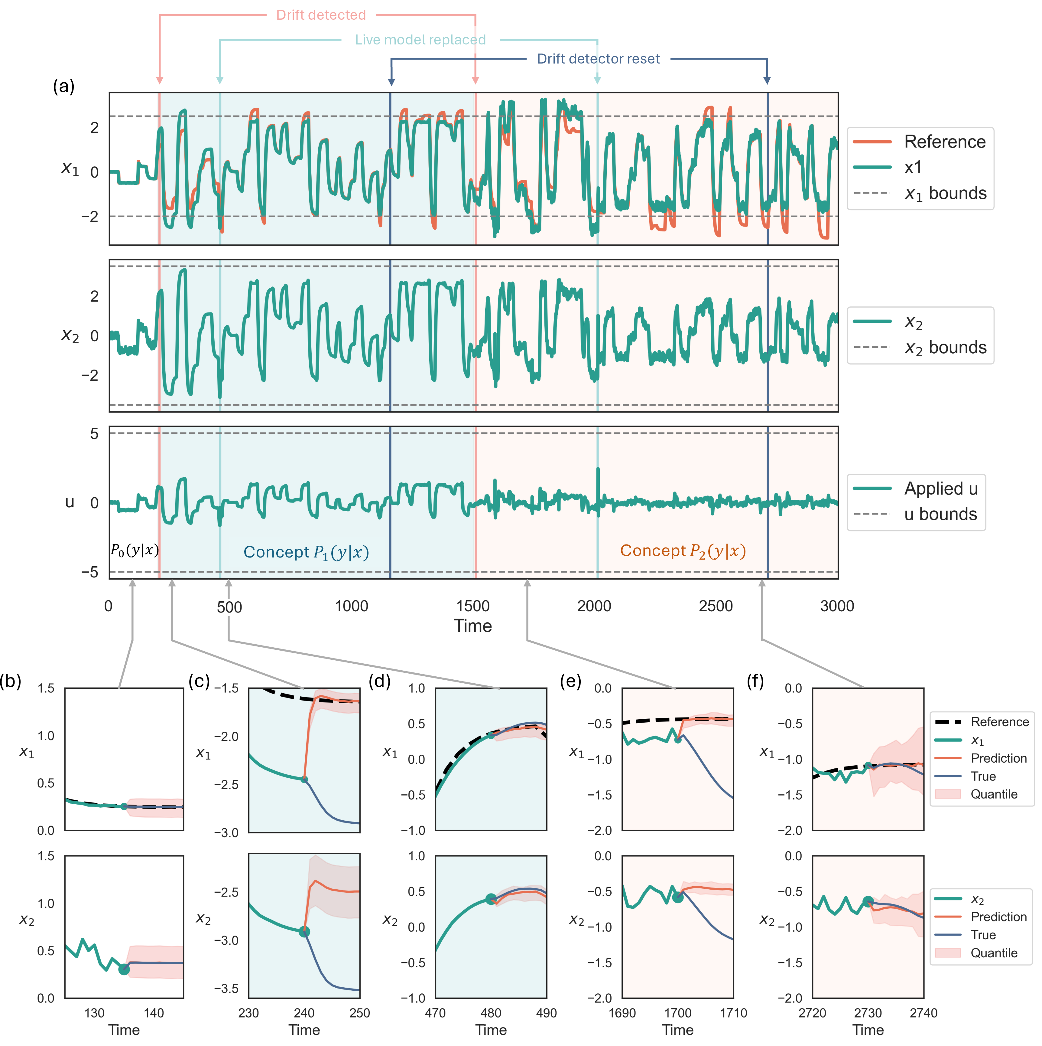
We show the resulting trajectory under the hybrid strategy, i.e.combining head fine-tuning with LoRA of rank \(r=1\), with buffer \(N_B=200\) and validation set \(N_V=30\). During fine-tuning, the learning rate is set to \(10^{-3}\) using the Adam optimizer. The model is trained for 100 epochs with a mini-batch size of 32. In addition, a
regularization term with coefficient \(2 \times 10^{-4}\) is incorporated into the loss function to mitigate overfitting. These hyperparameters are selected from preliminary experiments to ensure stable convergence and
effective adaptation but are not exhaustively optimized; their effect on adaptation performance can be case-dependent and is left to future work.
Figure 11 (a) shows the trajectories of \(x_1\) and \(x_2\) under the proposed adaptive Digital Twin framework. The results demonstrate effective drift detection and adaptation, restoring control performance under the injected uncertainties. Shaded regions denote different concept regimes, while drift detection, model replacement, and detector reset events are explicitly marked. The first drift (at \(k=200\)) is detected at \(k=207\) and the model is updated at \(k=456\), after which the detector resets at \(k=1156\). The second drift (at \(k=1500\)) is detected at \(k=1509\); the first update attempt fails validation, so a second update succeeds at \(k=2010\), with a detector reset at \(k=2710\).

Figure 11 (b)–(f) present the trajectories and quantile predictions in different regimes. In particular, the model predictions given the optimal control inputs are compared with the noise-free ground-truth state trajectories from Equation 15 . Before drift, the system accurately tracks the reference, and the TiDE predictions closely match the true trajectories (Figure 11 (b)). After the first concept drift, the pretrained model fails to capture the new dynamics, resulting in large prediction errors (Figure 11 (c)). Once drift is detected and the model is updated with data from the new regime, both prediction and control performance are restored (Figure 11 (d)). The updated TiDE also produces narrower predictive quantiles, indicating successful adaptation to the reduced aleatoric uncertainty.
At the second drift stage, the model again fails to capture the new dynamics (Figure 11 (e)) before being updated. After drift detection and adaptation, prediction accuracy is restored (Figure 11 (f)). Despite the increased noise variance, the updated TiDE accurately predicts the nominal trajectory while widening its predictive quantiles to reflect the higher aleatoric uncertainty. Overall, these results demonstrate that the proposed adaptive Digital Twin framework effectively detects and adapts to both types of drift, maintaining prediction and control performance.
The details of the fine-tuning process, validation performance, and the estimated \(T^2\) distribution after successful model updating are presented in Figure 12 (a)–(h). The first model update under concept \(P_1(y \mid x)\) is successful, as the validation loss of the idle model is statistically significantly lower than that of the live model according to the Mann–Whitney \(U\) test (Figure 12 (b)). Following the successful update and replacement of the live model, the drift detector is reset, and the estimated \(T^2\) distribution, along with its upper quantile, is updated using data collected from the new regime (Figure 12 (c)).
As the system transitions to concept \(P_2(y \mid x)\), the first model-update attempt is unsuccessful, with the null hypothesis not rejected despite the converged validation loss (Figure 12 (d)–(e)). Consequently, the drift detector is not reset, and the idle model continues to be updated as more data are collected. The second update attempt is successful (Figure 12 (f)–(g)), prompting the drift detector to reset and recalibrate the \(T^2\) distribution and its upper quantile using data from the new regime (Figure 12 (h)).
These results demonstrate that the proposed adaptive Digital Twin framework can autonomously detect drift, update and validate the surrogate model, and reset the drift detector using streaming data. The framework effectively adapts to changes in both the system dynamics (epistemic uncertainty) and the disturbance characteristics (aleatoric uncertainty). Overall, these results highlight the robustness and generality of the framework for reliable long-term deployment under evolving operating conditions.
4.5 Evaluation Metrics and Benchmarking↩︎
To jointly assess deterministic accuracy and the quality of the learned quantiles, we report four metrics evaluated against the nominal ground-truth responses: the normalized root mean square error (NRMSE), empirical coverage of the \(90\%\) prediction interval, the normalized negatively oriented interval score (NNOIS) [101], and the quantile loss. Together they characterize median accuracy, interval calibration, interval sharpness, and online learning quality; their full definitions are given in the Supplementary Information (SI).
| Method | Parameters | Detection | Fine-Tuning frequency | Validation | |
|---|---|---|---|---|---|
| No FT | No fine-tuning approach applied | — | |||
| Head FT | Fine-tuning the last layer every iteration, which is a common practice in most of the existing literature. | \(\alpha\)=1e-3 \(\lambda\)=1e-4 | Stepwise | ||
| Hybrid | Applying Head FT and LoRA (\(r=1\)) simultaneously and fine-tuning the model every iteration. | \(\alpha\)=1e-3 \(\lambda\)=1e-4 | Stepwise | ||
| LoRA | Applying LoRA (\(r=1\)) and fine-tuning the model every iteration. | \(\alpha\)=1e-3 \(\lambda\)=1e-4 | Stepwise | ||
| ADT Hybrid-N | Applying the proposed method with Hybrid method as the fine-tuning approach, but without online validation after fine-tuning. | \(\alpha\)=1e-3 \(\lambda\)=1e-4 \(N_B\)=200 \(N_{\text{epoch}}\)=100 | Batch | ||
| ADT Hybrid | Applying the proposed method with Hybrid method as the fine-tuning approach, with online validation after fine-tuning | \(\alpha\)=1e-3 \(\lambda\)=1e-4 \(N_B\)=200 \(N_V\)=30 \(N_{\text{epoch}}\)=100 | Batch | ||
| ADT LoRA-N | Applying the proposed method with LoRA (\(r=1\)) as the fine-tuning approach, but without online validation after fine-tuning | \(\alpha\)=1e-3 \(\lambda\)=1e-4 \(N_B\)=200 \(N_{\text{epoch}}\)=100 | Batch | ||
| ADT LoRA | Applying the proposed method with LoRA (\(r=1\)) as the fine-tuning approach, with online validation after fine-tuning. | \(\alpha\)=1e-3 \(\lambda\)=1e-4 \(N_B\)=200 \(N_V\)=30 \(N_{\text{epoch}}\)=100 | Batch | ||
| ADT LoRA-Ns | Applying the proposed method with LoRA (\(r=1\)) as the fine-tuning approach with a smaller batch size, with online validation after fine-tuning. | \(\alpha\)=1e-3 \(\lambda\)=1e-4 \(N_B\)=100 \(N_V\)=30 \(N_{\text{epoch}}\)=100 | Batch |

We benchmark the proposed Adaptive Digital Twin (ADT) framework, together with several of its variants, against existing online fine-tuning methods, as listed in Table 2. These benchmarks isolate the
effect of four design dimensions:
ADTvs.non-ADT: isolates the effect of the proposed framework relative to conventional fine-tuning. The key distinction is thatADTperforms drift-triggered, batch-wise adaptation, whereas the baseline methods update the model stepwise as each new observation becomes available.LoRAvs.Hybridvs.Head FT: comparesLoRA, which remains underexplored for adaptive model-based control, against conventional head fine-tuning, and examines whether the hybrid combination ofLoRAand head fine-tuning yields additional adaptation benefit. The same comparison is repeated within theADTframework by swapping only the fine-tuning module while holding all other components fixed.With validation vs.without validation: isolates the contribution of the proposed online validation stage, which safeguards against deploying an update that degrades predictive performance.
Larger vs.smaller batch size: examines the sensitivity of update quality to the size of the adaptation buffer.
For each approach, 30 replication simulations are conducted with different random seeds, and the distributions of NRMSE, Coverage, NNOIS, and the quantile loss \(L_Q\) of \(x_1\) and
\(x_2\) under adaptation to \(P_1\) and \(P_2\) are compared. For the ADT approaches, the evaluation metrics are not applied to the time
intervals occupied by the model-adaptation and model-validation stages, as this work focuses on the performance of the model after it is updated with statistical assurance. Although the Digital Twin’s performance may degrade during these stages, since the
live model is not fine-tuned immediately, once the model is fine-tuned and validated the predictive performance can outperform stepwise fine-tuning, providing an additional layer of trustworthiness under autonomous adaptation. The results across all
metrics are summarized in Figures 13–16, with the corresponding average ranks consolidated in Figure 17. Several consistent trends emerge across the two drifted
concepts.
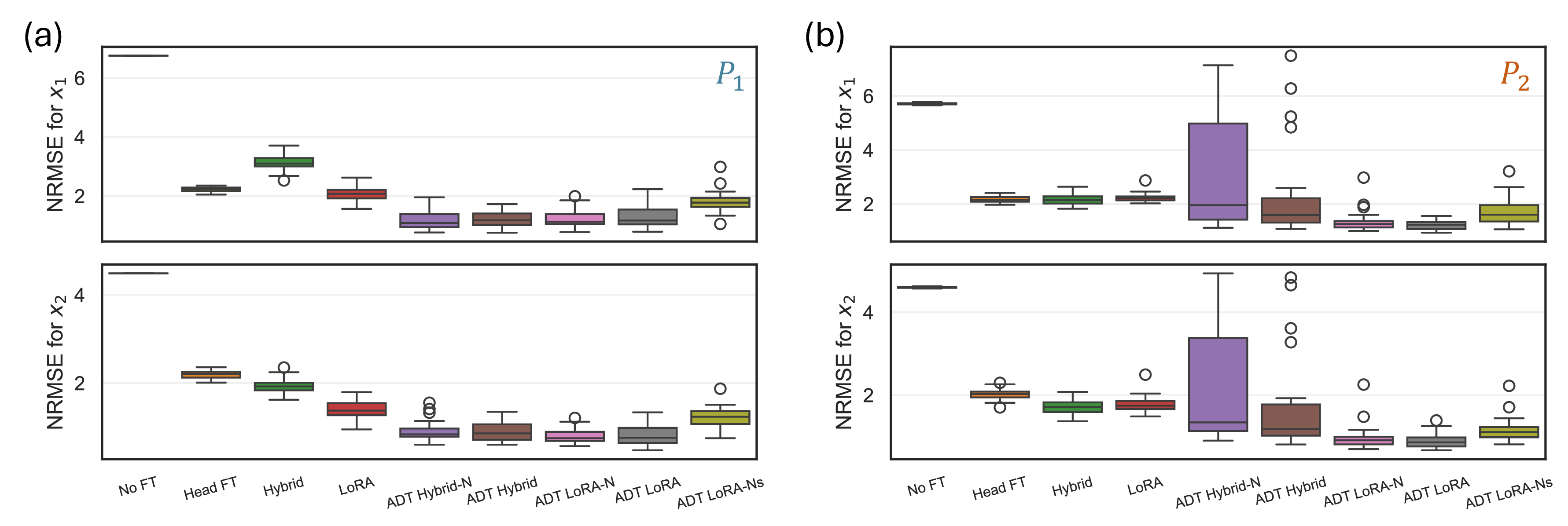

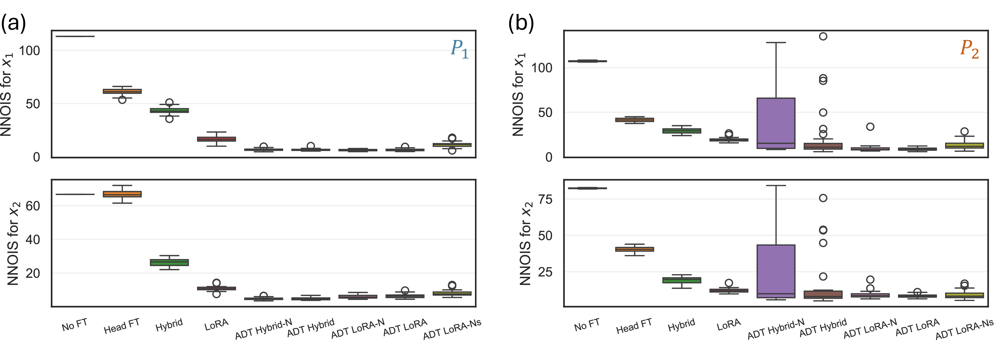
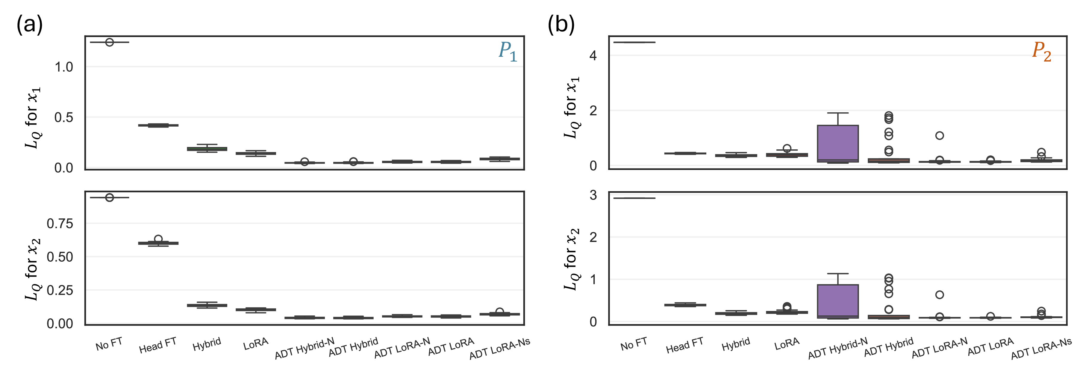

First, adaptation is essential: No FT ranks last under nearly every metric, and its coverage collapses toward zero (Figure 14), confirming that without updating the twin loses both accuracy and uncertainty
calibration once the regime shifts. Second, the ADT variants dominate the aggregate ranking despite their lower-frequency, batch-wise updates: ADT LoRA is best (average rank \(\approx 1.5\)),
followed by ADT LoRA-N (\(\approx 2.2\)), while the strongest stepwise baseline (LoRA, \(\approx 5.6\)) trails substantially, indicating that validated batch
updates yield better-calibrated quantiles than naive stepwise adaptation. Third, among fine-tuning strategies, head fine-tuning is weakest. By adjusting only output scaling and bias, it cannot capture the new dynamics and leaves coverage below nominal,
whereas LoRA and hybrid successfully recover the uncertainty estimates. Within ADT, ADT-LoRA slightly outperforms ADT-Hybrid, as its low-rank update supplies enough plasticity while its implicit regularization limits
overfitting on the small buffer, with the extra head parameters adding little in this low-dimensional example. Fourth, online validation matters most under \(P_2(y\mid x)\), where increased aleatoric uncertainty makes naive
updates risky. Without validation, ADT Hybrid-N degrades drastically, with heavy-tailed NRMSE outliers (Figure 13 (b)), whereas ADT Hybrid flags these failures via the validation module, updates the
model with additional cycles, and replaces the live model only with confidence. Finally, a larger buffer (\(N_B=200\)) outperforms the smaller one (\(N_B=100\)) under both concepts by
improving generalization and reducing sensitivity to transient samples. Overall, coupling score-based detection, LoRA adaptation, and statistical validation with a sufficiently large buffer gives the most accurate medians and best-estimated bounds under
both an abrupt dynamics change and a shift in aleatoric uncertainty.
5 Engineering Case Study on Additive Manufacturing↩︎
In this section, we apply the framework to DED as a case study, building on the testbed and dataset of [8], where the melt pool is a complex, highly nonlinear temporal system. Drift is injected via temperature-dependent material properties (e.g.thermal conductivity, specific heat), representing batch-to-batch feedstock variation. Unlike the explicit injection of the illustrative example, here the drift is embedded in the governing equations, producing nonlinear, non-additive effects on the dynamics and giving a more realistic and demanding test. We summarize the experimental setup, surrogate modeling and robust MPC, and finally the validation setup and results. The reader is referred to [8] for full DED Digital Twin details.
5.1 System Overview and Scope↩︎
The Digital Twin is designed for controlling melt pool dynamics, the most critical and controllable region of DED, where thermal history governs defects (porosity, lack of fusion, residual stress). The state is the melt pool temperature and depth, \(\mathbf{x}_k=[x_{\text{temp},k},x_{\text{depth},k}]^\top\), assumed observable via in-situ sensing, and the control input is the laser power \(u_k\).
The twin is a closed loop of (i) a physical system producing state observations, (ii) a virtual system producing multi-step predictions conditioned on candidate inputs, and (iii) an MPC computing the optimal action applied back to the plant. To maintain computational tractability for real-time decision-making, the Digital Twin is constructed at the melt pool level rather than the full part scale, reducing the dimensionality of the system while preserving the dominant dynamics relevant to control.
Detailed setup, data acquisition, and feature extraction are given in [6], [8]. Here we focus on integrating the DED system with the proposed framework, continuously monitoring and updating the surrogate under evolving conditions.
5.2 Physical System: GAMMA Simulation of DED Process↩︎
The physical DED process is represented by GAMMA, an in-house GPU-accelerated explicit FEA solver [102] performing part-scale transient heat-transfer simulation, providing a controlled environment [8] for generating trajectories and injecting uncertainties for virtual experiments. A single-track square geometry is selected as the target structure, illustrated in Figure 18, with detailed specifications provided in Table [tab:square95spec]. Here, an AISI 1018 substrate is used, and 316L stainless steel serves as the printing material. This setup enables efficient simulation of complex thermal dynamics while preserving sufficient fidelity in capturing melt pool behavior relevant to control. The single-track structure can also be used for future experimental verification of melt pool depths. For comprehensive details regarding the DED setup, feature extraction, and data-processing pipeline, the reader is referred to our previous work [8].

5.3 Virtual System: Surrogate Modeling via TiDE↩︎
To construct a sufficiently rich set of laser power trajectories, a time-series design of experiments is adopted to systematically explore the input space. Following the approach of [14], each laser power profile is parameterized in a reduced-dimensional representation using a Fourier basis, resulting in a 10-dimensional coefficient space. Latin Hypercube Sampling is then employed to generate diverse trajectories within this space, enabling broad coverage of admissible process variations. Additional implementation details can be found in prior studies [8], [14]. Based on this strategy, 100 distinct simulations are performed using the finite element model. At each timestep, key thermal responses, including melt pool temperature and depth, are recorded. The resulting dataset spans a wide range of operating conditions and provides sufficient variability for learning the underlying process–response mapping.
Using this dataset, a TiDE is trained as a multivariate, multi-step predictor. The model is configured with an input window size of \(w = 50\) and a prediction horizon of \(N = 50\), and predicts the 0.05 and 0.95 quantiles that define the lower and upper bounds, respectively. Detailed training procedures and hyperparameter settings are provided in [8]. The trained model achieves a MAPE of 1.29% and an RRMSE of 0.054 for melt pool temperature, and 4.25% and 0.0441, respectively, for melt pool depth.
The dominant source of aleatoric uncertainty in the generated data arises from numerical artifacts in the FEA. Specifically, the mismatch between the laser traversal distance per timestep and the mesh discretization produces inconsistent thermal exposure across elements, leading to significant fluctuations in temperature and melt pool geometry that can exceed those caused by external disturbances such as material variability. Although these fluctuations are reproducible under identical simulation settings, they cannot be readily reduced through additional sampling. The TiDE model addresses this by extracting dominant temporal patterns through its dense encoder to generate a smoothed median prediction, while capturing the remaining variability through learned quantile bounds.
5.4 Decision-Making: Robust MPC Formulation↩︎
The deployment of MPC in DED aims to enable anticipatory regulation of the thermal process so that porosity defects can be mitigated even under arbitrarily specified melt pool temperature references. Prior studies suggest that maintaining the melt pool depth within a dilution window of 10% to 30% is essential for preventing both interlayer and intralayer porosity [103]. Identically to our formulation in [6], the robust MPC is formulated to track the desired temperature trajectory while enforcing chance constraints on melt pool depth:
\[\tag{19} \begin{align} \min\limits_{\mathbf{u}} & \sum_{i=0}^{N-1} \left( \left|\hat{x}_{\text{temp},k+i+1} - r_{\text{temp},k+i+1}\right|_{\mathbf{Q}}^2 + \left|\Delta u_{k+i}\right|_{\mathbf{R}}^2 \right) \\ \text{s.t.} & \mathbb{P}\left(\hat{x}_{\text{depth},k+i} \geq x_{\text{depth,lb}}\right) \geq 0.95, \quad \forall i \in \mathbb{N}{[1,N]}, \tag{20}\\ & \mathbb{P}\left(\hat{x}_{\text{depth},k+i} \leq x_{\text{depth,ub}}\right) \geq 0.95, \quad \forall i \in \mathbb{N}{[1,N]}, \tag{21}\\ & [\hat{\mathbf{x}}_{\text{temp},k+1}^{f}, \hat{\mathbf{x}}_{\text{depth},k+1}^{f}]^T = \text{TiDE}(\mathbf{x}_{\text{temp},k}^{p}, \mathbf{x}_{\text{depth},k}^{p}, \mathbf{d}_{x,k}^{p:f}, \mathbf{d}_{y,k}^{p:f}, \mathbf{z}_k^{p:f}, \mathbf{u}_k^{p:f}), \\ & u_{k+i} \in \mathbb{U} := \left\{ u \in \mathbb{R} \mid 504~\text{W} \leq u_{k+i} \leq 750~\text{W} \right\} \end{align}\]
In this formulation, \(\Delta u_{k+i}\) penalizes variations in consecutive control inputs to encourage smooth laser power modulation. The auxiliary variables \(\mathbf{d}_x\) and \(\mathbf{d}_y\) denote the distances from the laser position to the nearest geometric boundaries along the \(x\)- and \(y\)-directions, while \(\mathbf{z}\) represents the nozzle height. These geometry-dependent quantities are incorporated as exogenous inputs to the TiDE model, improving its ability to capture spatially varying process dynamics. Unlike conservative robust MPC formulations that tighten the input constraints, no such modification is applied here, as the admissible input range remains inactive throughout the operating regime considered. Note that the constraint is enforced only from the fourth layer onward, as the melt pool temperature and depth are lower in earlier layers due to the boundary conditions imposed by the substrate.
5.5 Phase I: Drift Detector Setup↩︎
As before, the pretrained TiDE (796,594 parameters) is augmented with a linear head and LoRA layers. Here, we fine-tune only the LoRA layers (7,476 parameters with \(r=1\)) and freeze the last layer for parameter
efficiency. Since TiDE predicts both states over a 50-step horizon with three quantiles, the last-layer score is high-dimensional, giving a \(90{,}000\times 90{,}000\) covariance whose direct FULL inversion
(\(\mathcal{O}(n^3)\)) is intractable online; we therefore adopt DIAG as a robust, tractable trade-off.
To establish the reference distribution of the MEWMA statistic under in-control conditions, a separate dataset of size 6,000 is generated by running GAMMA under robust MPC with a temperature reference trajectory distinct from that used in online testing. The corresponding trajectories are shown in Figure 19. The first 3,000 samples are used to estimate the in-control score mean \(\bar{\mathbf{s}}\) and covariance matrix \(\hat{\Sigma}\), where \(\hat{\Sigma}^{-1}\) is approximated using only the inverse of its diagonal elements. The remaining 3,000 samples are then used to sequentially compute the Hotelling \(T^2\) statistic via MEWMA with \(\lambda = 0.02\), based on the estimated \(\bar{\mathbf{s}}\) and \(\hat{\Sigma}^{-1}\). The empirical distribution of \(T^2\) is subsequently approximated, and the detection threshold \(h\) is determined from the fitted distribution with bootstrapping at significance level \(\alpha = 10^{-4}\). The resulting \(T^2\) trajectory and its empirical distribution are shown in Figure 20 (a)–(b). The \(T^2\) statistic shows periodic peaks (Figure 20 (a)) induced by layer transitions, where prediction error rises; these inherent variations must be reflected in \(\bar{\mathbf{s}}\), \(\hat{\Sigma}\), and the threshold to avoid excessive false alarms at layer switches.
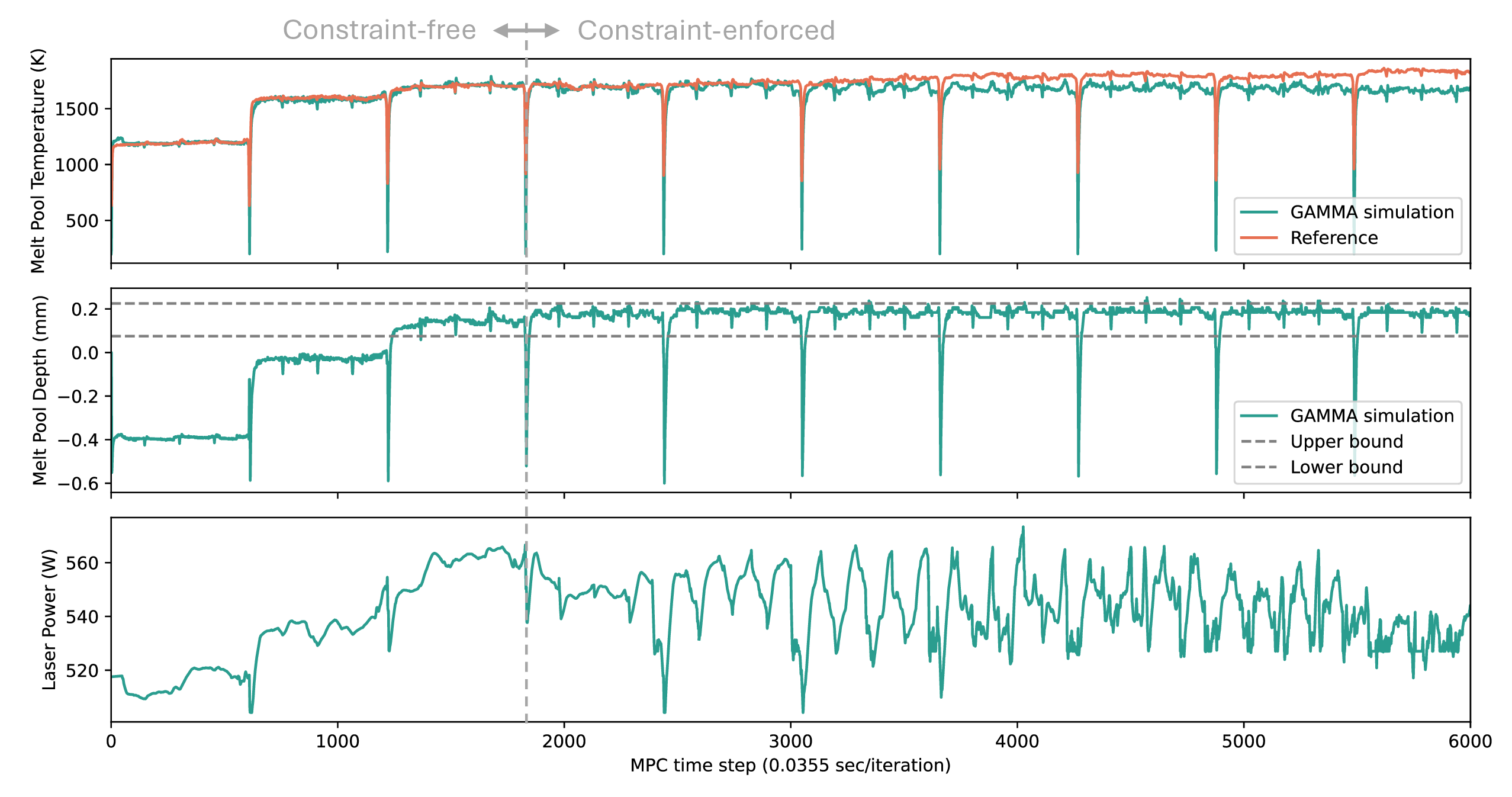
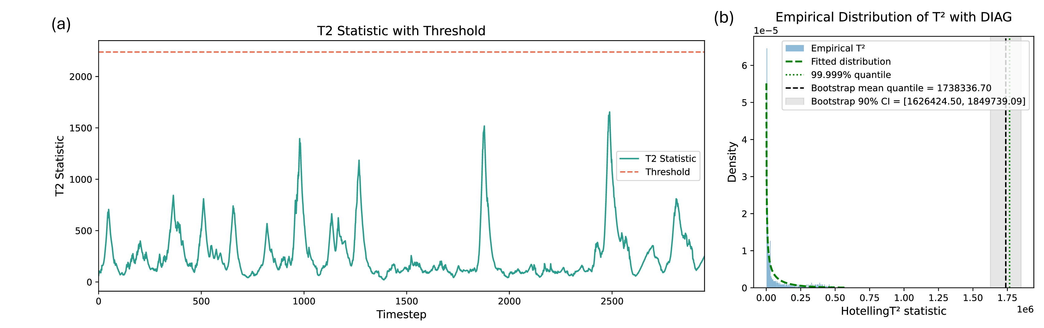
5.6 Drift Injection on Material Properties↩︎
The primary source of drift in the DED process arises from uncertainties in material properties. To evaluate the proposed framework under such conditions, variations are introduced into key material parameters, including density, solidus and liquidus temperatures, latent heat, and temperature-dependent thermal conductivity and specific heat capacity. Since 316L stainless steel is the printing material, the drift is applied to its properties to induce changes in the underlying system dynamics.
To realize this drift, a virtual mixture of 316L stainless steel and AISI 1018 is considered, where the effective material properties are computed as a weighted average of the two constituents. The mixing process is initiated at time step 2000, during which the weight of 316L is gradually reduced by 1.5% and replaced by AISI 1018 over 40 steps. This reduction continues until time step 2200, reaching a total decrease of 7.7%, after which the composition remains constant. The resulting static material properties of the mixture are summarized in Table 3, while the temperature-dependent thermal conductivity and specific heat capacity of both materials and their mixture are presented in Figure 21.
The discontinuities observed in the curves are intentionally introduced to calibrate the GAMMA simulation against experimental results. This adjustment is necessary because the GAMMA simulation accounts only for heat conduction, without incorporating phase change or fluid-flow effects, leading to a systematic overestimation of the melt pool temperature. It is important to note that this induced drift affects not only the material near the melt pool but the entire simulation domain, resulting in more pronounced changes than those observed experimentally. The purpose of this setup is not to replicate a specific physical scenario but to introduce a substantial, non-additive, and highly nonlinear perturbation to the system dynamics for rigorous evaluation of the adaptive framework.
| Material | Density (kg/mm\(^3\)) | Solidus temp. (K) | Liquidus temp. (K) | Latent heat (J/g) |
|---|---|---|---|---|
| SS 316L | 0.00798 | 1658.15 | 1673.15 | 290 |
| AISI 1018 | 0.00787 | 1693 | 1733 | 270 |
| Mixture (90% 316L, 10% AISI 1018) | 0.00800 | 1667.466 | 1684.451 | 289.62 |
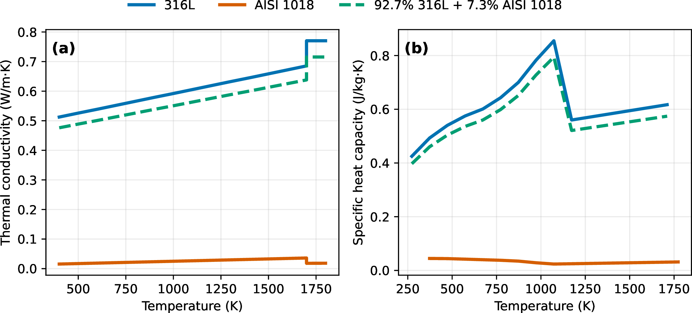
5.7 Phase II: Online Drift Detection, Adaptation, and Validation↩︎
Leveraging \(\bar{\mathbf{s}}\) and \(\hat{\Sigma}\) estimated from Phase I, the drift detector is deployed for online monitoring. As in the previous case, to reduce detection latency, only the quantile loss of the one-step-ahead prediction is used to represent the likelihood of the model. Once drift is detected, a data buffer of size 300 is collected for model fine-tuning. The fine-tuning procedure and associated hyperparameters remain identical to those used in the illustrative example. After successful fine-tuning, an additional 50 data points are collected during the validation stage to compare the quantile-loss distributions of the live and idle models. If the idle model passes the hypothesis test, it replaces the live model online, and the drift detector is reset. For the online reinitialization of Phase I, 200 data points are first collected to estimate \(\bar{\mathbf{s}}\) and \(\hat{\Sigma}\), followed by an additional 500 data points to estimate the distribution of the \(T^2\) statistic and its upper quantile, which serves as the alert threshold.
5.7.1 Unconstrained Model Predictive Control↩︎
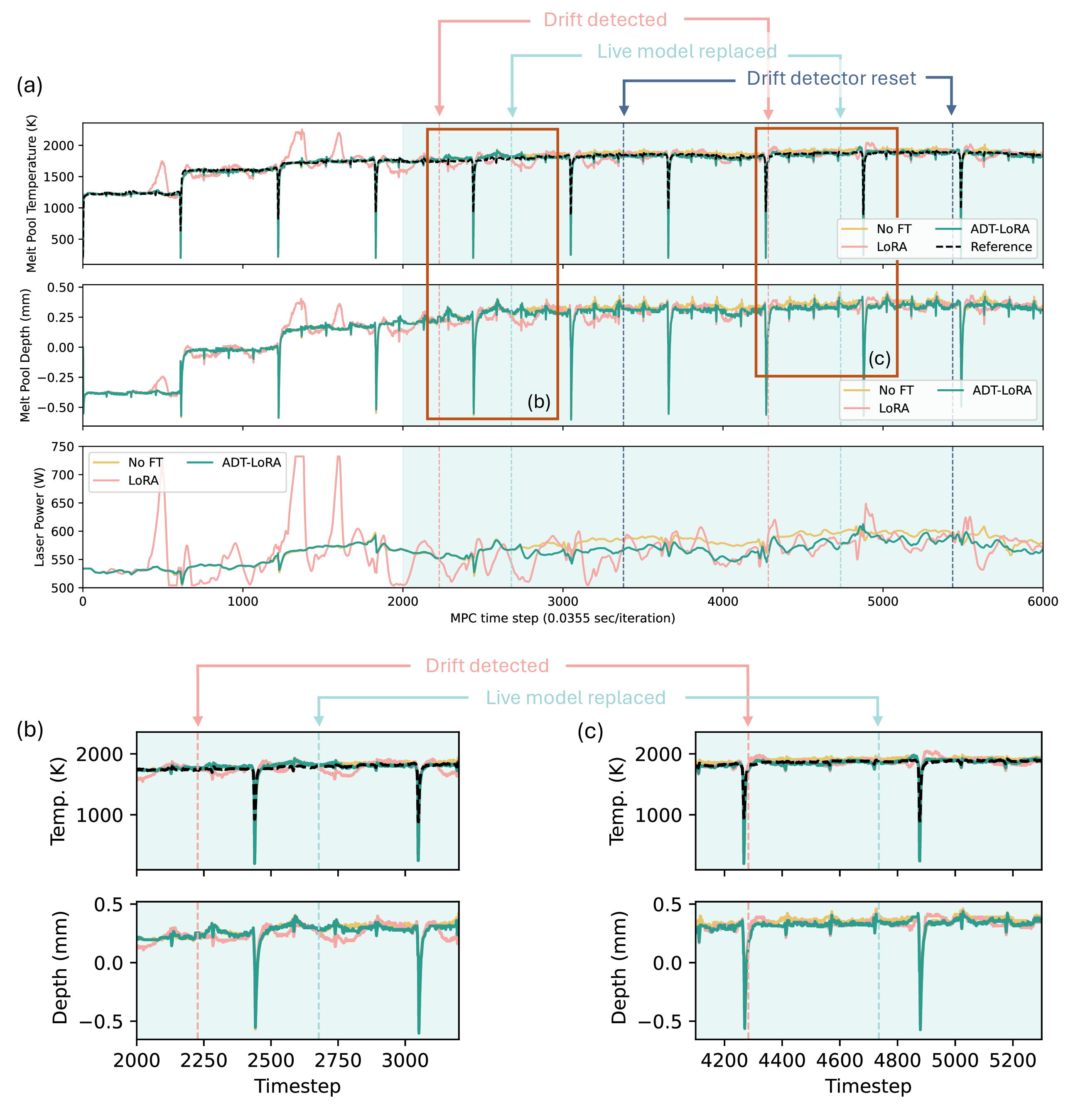
To begin with, we demonstrate the proposed method in unconstrained MPC, treating the process as a reference treacking problem by ignoring the melt pool depth constraints in Equation 19 . Figure 22 presents the trajectories of melt pool temperature, melt pool depth, and applied laser power throughout the drift-injected DED process simulated in GAMMA. The result of ADT-LoRA is shown, along with
No-FT and LoRA as benchmarks. As shown in Figure 22 (a), drift is first detected approximately 200 time steps after the material perturbation is introduced. Since the material drift is imposed
gradually and the effect of the graded material requires several time steps to become significant in the simulation, the detector remains effective, identifying drift before the discrepancy between the temperature trajectory and the reference becomes
pronounced (around time step 2,250). Although the comparison between the reference and state trajectories does not directly quantify prediction error, it reflects the degradation in control performance caused by an inaccurate predictive model within MPC.
Figures 22 (b) and 22 (c) highlight the region where drift is detected and the live model is subsequently replaced. As observed in these subfigures, the reference-tracking performance
(i.e.the discrepancy between the reference dashed line and the melt pool trajectory) improves significantly after the model update, demonstrating the capability of the proposed framework to maintain decision quality through effective online model
adaptation.
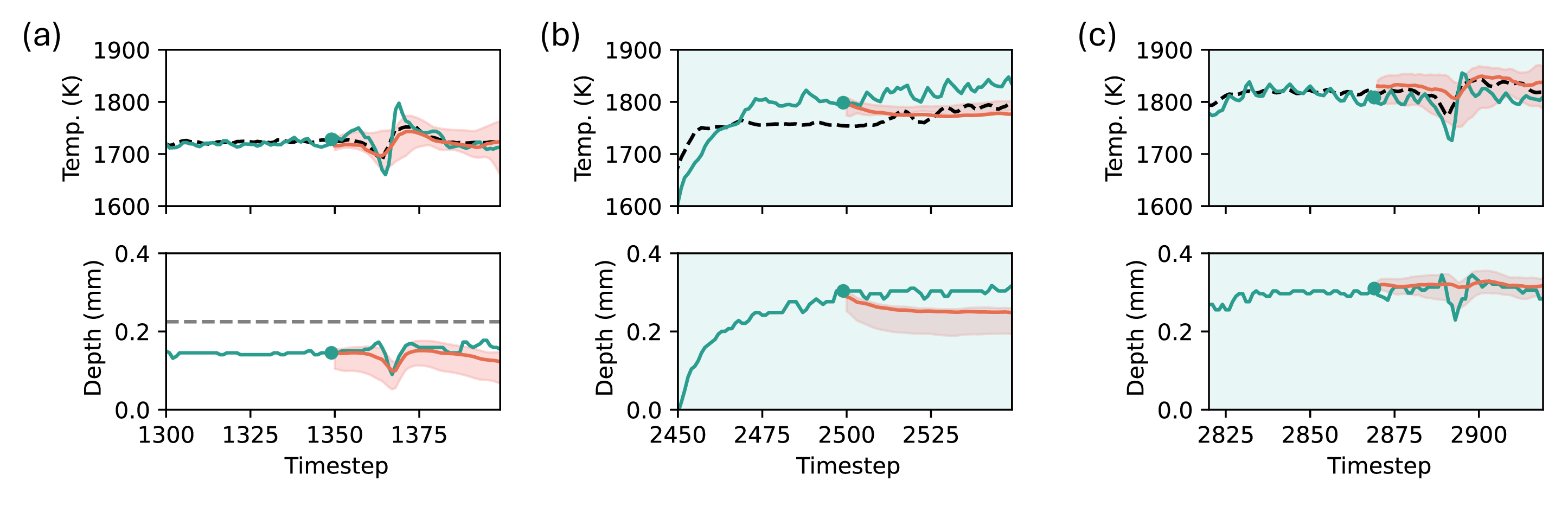
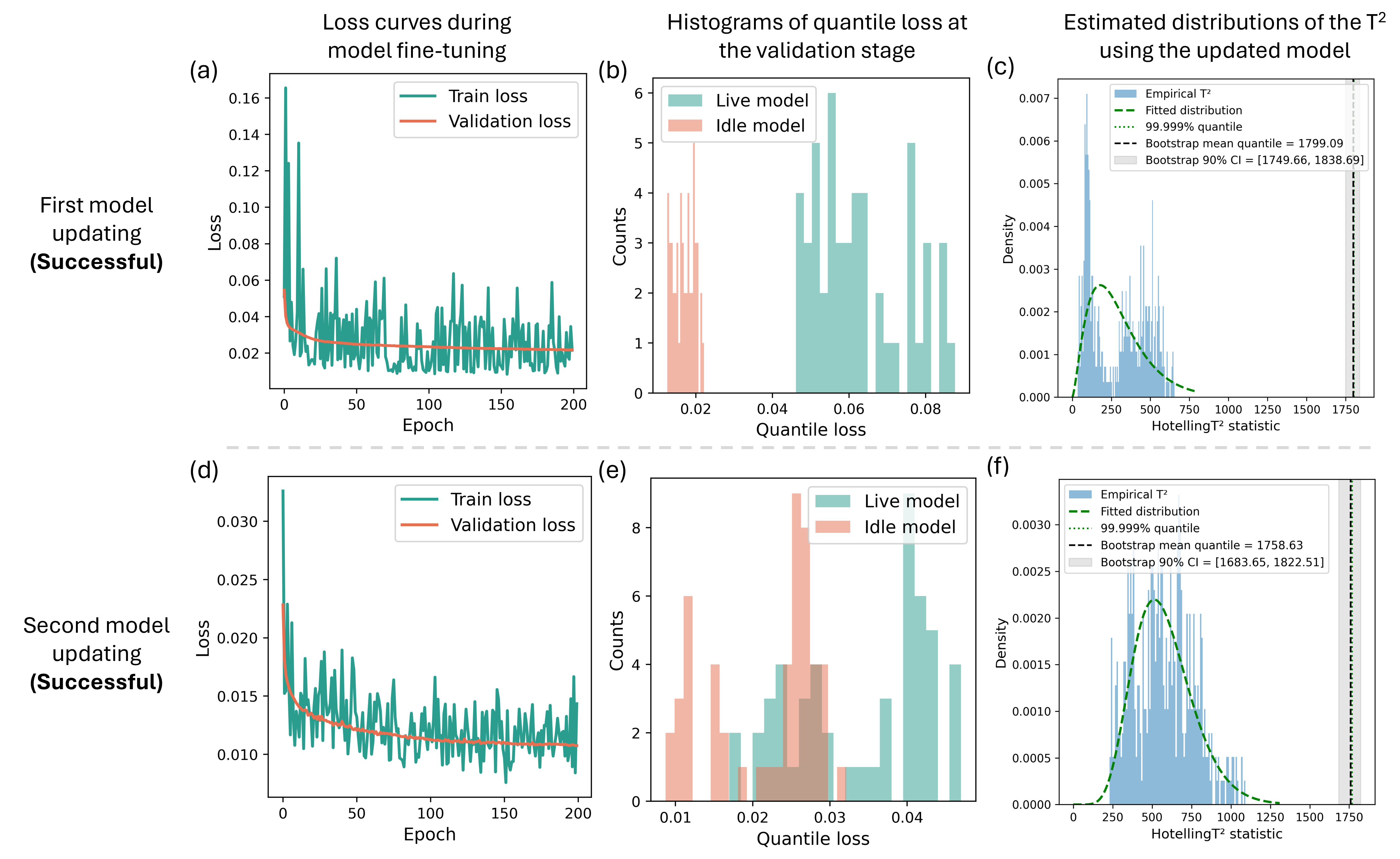
Compared to No FT and LoRA, ADT-LoRA offers several advantages. First, it achieves the best reference-tracking performance, attaining \(R^2 = 0.9168\) and \(\mathrm{MAE} = 33.6988\)K against the temperature reference trajectory after the material drift is injected. In comparison, No FT and LoRA yield \(R^2 = 0.9064\) and
\(0.8580\) with \(\mathrm{MAE} = 56.5141\) and \(43.2749\), respectively, reflecting larger tracking errors. The degradation is especially pronounced for
LoRA, where stepwise fine-tuning introduces substantial instability even before the drift occurs, producing severe overshoot and poor tracking. Moreover, once the drift is injected, the iterative updates degrade the surrogate further,
amplifying the fluctuations in both melt pool temperature and laser power. The improvement over No FT is more modest, but Figure 22 shows that its melt pool temperature remains mostly above the reference,
consistent with its larger \(\mathrm{MAE}\), and its laser power exceeds that of ADT-LoRA, since the un-adapted model is unaware of the material change that lowers the energy required to heat the melt pool.
Overall, the proposed method delivers both superior tracking accuracy and greater stability under continuous model updating.
Figure 23 (a)–(c) shows predictions before drift, under drift before updating, and after adaptation. Because the realized and multi-step-predicted trajectories use different inputs, the comparison is qualitative. In Figure 23 (a) the quantiles capture the variability and the median follows the trend. In Figure 23 (b) the mismatched model underestimates temperature and depth, as the injected drift lowers solidus temperature, conductivity, and specific heat, raising melt-pool temperature and depth at fixed power. After successful model updating, the mismatch is mitigated, as shown in Figure 23 (c): the predictive quantiles once again capture the fluctuations of the state trajectories, and reference-tracking performance is effectively restored.
Note that drift is also detected at time step 4,268 despite the absence of additional perturbations. As shown in Figure 24 (a)–(f), fine-tuning successfully improves the model predictions, as evidenced by the validated quantile-loss distributions. This behavior stems from the inherently non-stationary DED process, where the nozzle height continuously increases while model updates rely on data from a localized region. This observation highlights an advantage of score-based drift detection in non-stationary settings: an increase in the score-vector magnitude indicates not only reduced confidence in the parameter estimates under drifted stationary conditions but also elevated epistemic uncertainty arising from insufficient knowledge in evolving operating regimes.
5.7.2 Constrained Robust MPC↩︎

We revisit the same drift-injected process under constrained robust MPC, where chance constraints restrict the melt-pool depth to the \(10\%\)–\(30\%\) dilution window, enforced from the
fourth layer, using ADT-LoRA, with No FT and LoRA as benchmarks. With constraints enforced, drift is detected \(\approx 300\) steps after the material perturbation begins.
Figure 25 (a) compares the three approaches. ADT-LoRA handles constraints best, keeping the depth below the upper bound at the lowest violation rate (\(14\%\))
throughout the entire printing process, including the adaptation period. The zoomed views in Figure 25 (b)–(c) show that after each model replacement the depth is driven away from the active constraint,
creating margin for fluctuations and reflecting successful adaptation of the constraint-enforcing quantiles. In contrast, although LoRA attains an \(18\%\) violation rate, its iterative updates cause repeated
overshoots at layer transitions and hold the depth overly far from the constraint, exhibiting over-conservativeness. Lastly, No FT underestimates the melt pool depth once drift occurs, incurring a \(46\%\)
violation rate. Thus ADT-LoRA adapts more robustly while maintaining constraint satisfaction.
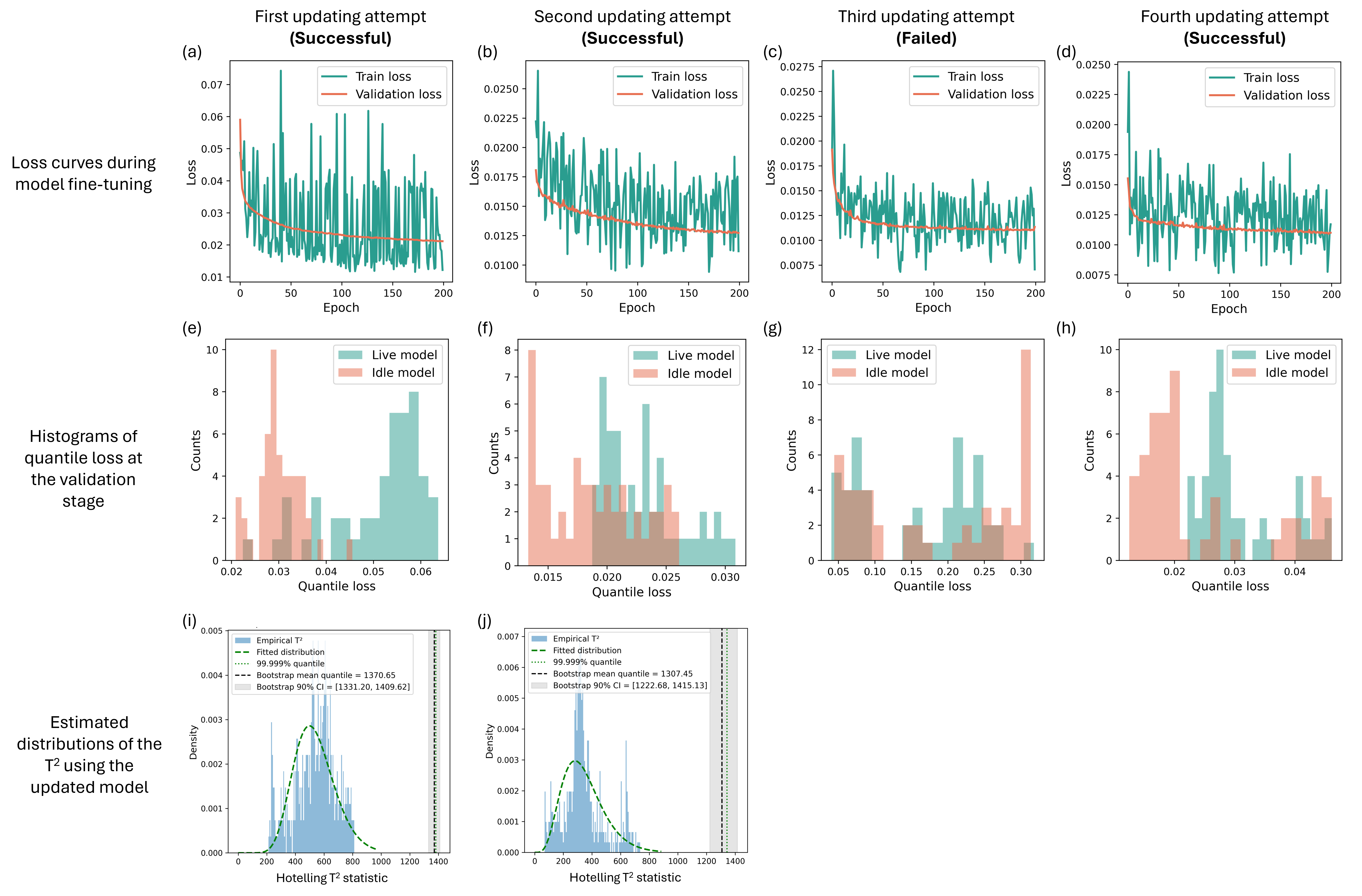
Figure 26 (a)–(j) presents the fine-tuning loss curves, the validation-stage quantile-loss histograms for the live and idle models, and the fitted \(T^2\) distributions used
to reset the drift detector after successful updates. Throughout the print, ADT-LoRA detects drift three times and performs four fine-tuning attempts: the third fails validation and triggers re-adaptation, while the fourth succeeds, but the
third detector reset cannot be completed before the print ends. The frequent detections are partly due to increased out-of-distribution (OOD) inputs, as the unconstrained offline training data differ from the operating distribution under constrained
control, causing the detector to respond to both covariate and concept drift.
Finally, Figure 27 shows the drift-detection computation time measured on an AMD Ryzen Threadripper PRO 3975WX CPU with a single NVIDIA A6000 GPU. Fine-tuning time is excluded, as it can be performed in parallel on separate hardware without affecting system operation. Score-based detection typically completes in under \(0.008\) s, with a few instances reaching \(0.012\) s, yielding an average detection time of \(0.0075\) s per step, well within the 35.5ms control interval. Since the computation mainly involves a single forward and backward pass, its inference cost scales with the size and structure of the model.

Taken together, the unconstrained and constrained DED studies show that the proposed framework transfers from the illustrative linear system to a complex, highly nonlinear, non-stationary manufacturing process in which the injected drift is embedded in
the governing physics and perturbs the dynamics non-additively. Each of the three design pillars is borne out. For when to update, score-based detection identifies the gradual material drift well before control degrades and additionally flags the
out-of-distribution behavior induced by the inherently non-stationary build. For how to update, LoRA restores not only the median prediction but also the quantile bounds, enabling the framework to recover reference tracking in the unconstrained
setting and to enforce the dilution constraint in the constrained setting. For whether the update succeeds, online validation blocks unsuccessful updates in the constrained case. Crucially, these gains hold across two distinct decision-making
objectives and against benchmarks that either fail to adapt (No FT, systematically biased) or adapt naively (stepwise LoRA, unstable and overly conservative), confirming that drift-triggered, batch-wise, validated adaptation is
more robust than either extreme. Combined with a sub-\(10\) ms detection cost, the case study establishes the framework as a practical, real-time-capable add-on for sustaining the fidelity of NN-based Digital Twins under
previously unseen operating conditions. Owing to the high computational cost of the high-fidelity FEA simulations, the DED case study reports single-run results and is intended to demonstrate framework transferability, whereas statistical robustness of the
methodological choices is established in the 30-replication illustrative study.
6 Closure↩︎
In this work, an online adaptation framework for Digital Twins is proposed. Building upon real-time decision-making algorithms such as Model Predictive Control (MPC), the framework incorporates a drift-detection mechanism to address when to update the model, parameter-efficient fine-tuning to determine how to update the model, and hypothesis testing for online validation to assess whether the update is successful. A concrete, generalizable realization is demonstrated through the integration of score-based drift detection, LoRA-based adaptation, and the Mann–Whitney \(U\) test, with neural networks serving as surrogate models.
Two case studies verify the effectiveness of the proposed approach, both employing quantile-based robust MPC as the uncertainty-aware decision-making algorithm. In an illustrative example with injected abrupt uncertainty, the model is effectively fine-tuned during operation to accommodate both epistemic and aleatoric uncertainties. In an engineering case study on Directed Energy Deposition additive manufacturing, the framework adapts to incremental drift in material properties while maintaining control performance. These case studies collectively indicate that the proposed framework provides an effective and rigorous approach for maintaining the trustworthiness of Digital Twins under previously unseen conditions, thereby enhancing their ability to handle unknown uncertainties.
Although the proposed framework establishes a statistically rigorous pipeline for online adaptation, it introduces a trade-off in responsiveness, as the adaptation speed to drift is slower than that of stepwise, iterative model-updating methods commonly used in adaptive MPC with high-frequency decision requirements. To mitigate the impact of model mismatch during the adaptation phase, ad hoc compensation strategies such as offset-free control algorithms [104] can be incorporated. In addition, [105] presents a promising perspective, demonstrating that accurate control performance may still be achieved with an imperfect model through alignment of the optimality conditions governing control actions. These approaches are suited as interim compensation strategies when model accuracy is degraded. Moreover, because the primary focus of this work is model adaptation from a fine-tuning perspective, control-oriented considerations, such as enforcing stability through Lyapunov-based constraints [46], [106], are not incorporated into the model-updating criteria. Consequently, the proposed framework does not provide formal guarantees on MPC stability. However, robust MPC stability guarantees depend on the surrogate model through its prediction-error bound and therefore remain applicable to updated models that satisfy the same bound. Control-theoretic certification and validated model adaptation thus play complementary roles. The former supports closed-loop guarantees, while the latter helps maintain the Digital Twin’s fidelity to an evolving physical system.
This work establishes a foundation for model adaptation through a score-based drift-detection approach, offering promising potential for diagnosing parametric black-box models while introducing a degree of interpretability. With the capability to monitor individual parameters or groups of parameters, it can naturally be extended to enable autonomous adaptation and drift management in Digital Twins of complex systems, or even systems of systems. In particular, it provides a pathway to identify and localize drifting parameters, thereby focusing model updates on the most relevant subsets of the system.
Such capabilities can further enhance the trustworthiness of Digital Twins by improving interpretability, especially when coupled with more transparent model representations such as differentiable causal modeling and analysis. Building on this foundation, methods such as reinforcement learning [70] can be incorporated to scale the framework to more complex decision-making settings, enabling the system to handle emergent behaviors through integrated reasoning and diagnosis within the surrogate model. This progression ultimately contributes to advancing machine intelligence in autonomous Digital Twin systems.
Acknowledgement↩︎
We are grateful for the grant support from the National Science Foundation’s Engineering Research Center for Hybrid Autonomous Manufacturing: Moving from Evolution to Revolution (ERC-HAMMER), under Award Number EEC-2133630. Yi-Ping Chen acknowledges the Taiwan-Northwestern Doctoral Scholarship, and Seul Lee acknowledges the Samsung Electronics Doctoral Scholarship.
Declaration of Generative AI Use↩︎
During the preparation of this work, the authors used Claude and ChatGPT in order to improve the language, readability, and clarity of the manuscript. After using this tool, the authors reviewed and edited the content as needed and take full responsibility for the content of the publication.
References↩︎
Corresponding author, weichen@northwestern.edu, Department of Mechanical Engineering, Northwestern University, Evanston, IL, 60208↩︎