Manifold-Constrained Hyper-Connections for Parameter-Efficient Finetuning
July 20, 2026
Abstract
Most parameter-efficient finetuning (PEFT) methods adapt weights or activations, thus leaving one of the key Transformer components unchanged: residual connections. This paper investigates Manifold-Constrained Hyper-Connections (mHC), a generalisation of residual connections, as a novel PEFT approach, wrapping frozen OLMo-2 backbones with learned residual routing modules. We find that mHC can finetune frozen Transformers, but that its role differs fundamentally from the original pre-training setting: in finetuning, fixing the residual mixing matrix to identity often improves performance. As a standalone PEFT method, mHC does not consistently outperform LoRA. However, at matched trainable parameter budgets, mHC+LoRA combinations improve language-modelling loss and show task-dependent benchmark gains at both 1B and 7B scale. Overall, our results identify residual routing as a distinct and promising novel PEFT axis.
1 Introduction↩︎

Rather than training models from scratch, many modern deep learning systems leverage foundation models: large models pre-trained on large-scale datasets. These models are subsequently finetuned for specific downstream tasks [1]. Finetuning is a form of transfer learning, but updating all parameters of a large model can be inefficient and risks catastrophic forgetting [2]. Parameter-efficient finetuning (PEFT) addresses this by freezing the backbone and training only a small number of additional parameters [3]. Adapter methods introduce small trainable modules [4]. LoRA, for example, updates selected weight matrices via low-rank decomposition [5]. These methods can be effective, but they mostly adapt weights or add modules while leaving the model’s architecture, such as its residual connections, unchanged.
Residual connections [6] add an identity path to each layer and are usually written as \[\label{eq:residual95connection} \mathbf{z}^{l} = f^{l}(\mathbf{z}^{l-1}) + \mathbf{z}^{l-1},\tag{1}\] where \(\mathbf{z}^{l-1}, \mathbf{z}^{l} \in \mathbb{R}^{d}\) are the input and output representations of layer \(l\), and \(f^{l}: \mathbb{R}^{d} \to \mathbb{R}^{d}\) is the learned transformation at that layer. They made deep networks easier to train by addressing the vanishing gradient problem: by creating a shortcut between input and output, gradients can propagate more easily. This helps to preserve important features and patterns in the data, see, e.g., [7]. Another benefit is that shorter paths through the network help route information over layers [8]. Due to their effectiveness, residual connections have become a standard practice in deep networks [9].
Recently, [10] introduced flexibility into the simple form of Eq.@eq:eq:residual95connection with Hyper-Connections (HC), a generalisation of the residual connection. It allows the model to learn how representations at different depths should interact. HC is highly parameter-efficient: for \(n\) as the number of streams (typically set to 4), the hyper-connection adds only \(n^2 + 2n = 24\) parameters per layer. While this mechanism increases the expressivity of the model, it also removes the stability guarantee of an identity path. HC has unconstrained residual mixing coefficients, which can compound over depth and amplify or suppress the residual stream. HC can thus become unstable and difficult to scale.
[11] address this with Manifold-Constrained Hyper-Connections (mHC). mHC keeps the same learned residual mixing as HC, but constrains the residual matrix to lie on a norm-preserving manifold that prevents the instability an unconstrained matrix can otherwise introduce over depth. By doing so, mHC keeps the flexibility of learned routing while preventing the destabilising of residual streams. In pre-training, mHC improves over HC and other residual-connection baselines with limited additional overhead [11]. However, its potential for finetuning foundation models remains unexplored.
We address this gap by exploring whether mHC can be applied as a PEFT method: we wrap a pre-trained Transformer backbone with an mHC module.1 Unlike PEFT methods that adapt selected weights or insert local trainable modules, mHC wraps the residual connections with either a static or dynamic learned transformation, modifying how intermediate representations are scaled or projected before being added back to the residual stream. In other words, it combines information across residual streams and depths, rather than just changing local transformations inside individual layers. Figure 1 depicts an original MLP layer with residual connection, a layer with an mHC-wrapper, and a layer with a LoRA-wrapper. Because it targets a different mechanism, mHC may serve both as a lightweight PEFT method on its own and as a complement to existing PEFT methods.
Overall, this paper makes five contributions: (i) we introduce mHC as a PEFT mechanism for frozen Transformer backbones, shifting it from its original pre-training setting to finetuning; (ii) we compare static and dynamic mHC variants against standard PEFT baselines; (iii) we identify identity preservation as the main mechanistic finding, showing that fixing learned residual mixing to identity improves or preserves performance while reducing trainable parameters; (iv) we evaluate mHC as a complement to existing PEFT methods, finding that mHC+LoRA can improve language-modelling loss and gives task-dependent downstream gains; and (v) we scale selected experiments to larger 7B scale.
2 Background↩︎
As seen in Eq. 1 , residual connections give each layer an identity path in addition to its transformation \(f^{l}\). In Transformer blocks [12], normalisation placement determines how direct this path is. In post-norm, layer normalisation (LN) is applied after the residual addition \[\label{eq:post95norm} \mathbf{z}^{l}=\operatorname{LN}\!\left(\mathbf{z}^{l-1} + f^{l}(\mathbf{z}^{l-1})\right).\tag{2}\] Pre-norm blocks, which preserve a more explicit residual stream, apply normalisation inside the \(f^{l}\) branch \[\label{eq:pre95norm} \mathbf{z}^{l}=\mathbf{z}^{l-1}+f^{l}\!\left(\operatorname{LN}(\mathbf{z}^{l-1})\right).\tag{3}\] This creates trade-off between pre-norm variants, where highly similar features in deeper layers can lead to representation collapse, and post-norm variants, where vanishing gradients may be reintroduced [13]. This distinction matters for HC and mHC because both modify how the residual stream is routed over depth.
2.1 Hyper-Connections↩︎
HC generalises the single residual stream in Eq. 1 by maintaining \(n\) residual streams [10]. Let \[\mathbf{Z}^{l-1} = \begin{bmatrix} \mathbf{z}^{l-1}_{1} \\ \vdots \\ \mathbf{z}^{l-1}_{n} \end{bmatrix} \in \mathbb{R}^{n \times d}\] denote these \(n\) streams before layer \(l\), where each \(\mathbf{z}^{l-1}_{i} \in \mathbb{R}^{d}\). HC reads from the streams using \(\mathbf{h}^{l}_{\mathrm{pre}} \in \mathbb{R}^{n}\): \[\mathbf{x}^{l}=(\mathbf{h}^{l}_{\mathrm{pre}})^{\top}\mathbf{Z}^{l-1} \in \mathbb{R}^{d}.\] The layer output \(f^{l}(\mathbf{x}^{l})\) is written back using \(\mathbf{h}^{l}_{\mathrm{post}} \in \mathbb{R}^{n}\), while \(\mathbf{H}^{l}_{\mathrm{res}} \in \mathbb{R}^{n \times n}\) mixes the residual streams: \[\label{eq:hc95update} \mathbf{Z}^{l} = \mathbf{H}^{l}_{\mathrm{res}}\mathbf{Z}^{l-1} + \mathbf{h}^{l}_{\mathrm{post}} \otimes f^{l}(\mathbf{x}^{l}),\tag{4}\] where \(\otimes\) denotes the outer product that writes the layer output into each stream by \(\mathbf{h}^{l}_{\mathrm{post}}\). Here, \(\mathbf{h}^{l}_{\mathrm{pre}}\), \(\mathbf{H}^{l}_{\mathrm{res}}\), and \(\mathbf{h}^{l}_{\mathrm{post}}\) are the effective routing objects. In static HC, they are obtained from learned logits \(\tilde{\mathbf{h}}^{l}_{\mathrm{pre}}\), \(\tilde{\mathbf{H}}^{l}_{\mathrm{res}}\), and \(\tilde{\mathbf{h}}^{l}_{\mathrm{post}}\).
This construction lets the model learn how to route representations across residual streams and depths. Moreover, HC is also extremely efficient in parameters. For expansion rate \(n\), static HC learns \(n^{2}+2n\) routing logits per layer: \(n^{2}\) for \(\tilde{\mathbf{H}}^{l}_{\mathrm{res}}\), and \(n\) for both \(\tilde{\mathbf{h}}^{l}_{\mathrm{pre}}\) and \(\tilde{\mathbf{h}}^{l}_{\mathrm{post}}\). The drawback is that the effective mixing matrix \(\mathbf{H}^{l}_{\mathrm{res}}\) is not constrained to preserve the stability of the identity path. When Eq. 4 is unrolled over many layers, repeated products of these matrices amplify or suppress the residual streams, leading to unstable representations or gradients.
2.2 Manifold-Constrained Hyper-Connections↩︎
mHC by [11] addresses the instability of HC by constraining \(\mathbf{H}^{l}_{\mathrm{res}}\). The used constraint is doubly stochasticity: a matrix \(\mathbf{H}^{l}_{\mathrm{res}} \in \mathbb{R}^{n \times n}\) is doubly stochastic iff all its entries are nonnegative, i.e., \((\mathbf{H}^{l}_{\mathrm{res}})_{ij} \geq 0\), and all rows and columns sum to one, i.e., for all \(i,j \in \{1,\ldots,n\}\), \[\label{eq:doubly95stochastic} \sum_{j=1}^{n}(\mathbf{H}^{l}_{\mathrm{res}})_{ij} = 1, \qquad \sum_{i=1}^{n}(\mathbf{H}^{l}_{\mathrm{res}})_{ij} = 1.\tag{5}\] The set of doubly stochastic matrices is known as the Birkhoff polytope \(\mathcal{B}_{n}\) [14], [15]. mHC approximately projects the unconstrained residual mixing matrix onto this manifold using the Sinkhorn-Knopp algorithm [11], [16]: \[\label{eq:mhc95sinkhorn} \mathbf{H}^{l}_{\mathrm{res}} = \operatorname{Sinkhorn}\!\left( \tilde{\mathbf{H}}^{l}_{\mathrm{res}} \right),\tag{6}\] where \(\tilde{\mathbf{H}}^{l}_{\mathrm{res}} \in \mathbb{R}^{n \times n}\), which we describe in Appendix 12. Intuitively, the projection turns an arbitrary mixing matrix into a normalised routing matrix: each input stream distributes its signal across output streams, and each output stream receives a normalised signal. This reflects the constraints of Eq. 5 .
Through this normalisation, streams can still exchange information, but the router can no longer freely grow or shrink the residual signal across depth. At the same time, the identity property of the original residual connection is preserved (which we verify in Appendix 10). Empirically, [11] show that mHC keeps activations and gradients stable across layers, while unconstrained HC can amplify them substantially (see Figures 9 and 10 in Appendix 18).
Static mHC.For the static variant used in our experiments, the remaining routing objects are obtained from learned logits as \[\label{eq:static95mhc95maps95main} \begin{align} \mathbf{h}^{l}_{\mathrm{pre}} &= \sigma\!\left( \tilde{\mathbf{h}}^{l}_{\mathrm{pre}} \right), \\ \mathbf{h}^{l}_{\mathrm{post}} &= 2\sigma\!\left( \tilde{\mathbf{h}}^{l}_{\mathrm{post}} \right), \end{align}\tag{7}\] where \(\sigma(\cdot)\) is the element-wise sigmoid function and \(\tilde{\mathbf{h}}^{l}_{\mathrm{pre}}, \tilde{\mathbf{h}}^{l}_{\mathrm{post}} \in \mathbb{R}^{n}\). Together, Eq. 6 and Eq. 7 give the constrained routing objects used in the HC update, Eq. 4 . The update, therefore, keeps the same read-in, write-out, and residual-mixing structure as HC, but now uses a doubly stochastic residual mixing matrix. Since products of doubly stochastic matrices remain doubly stochastic, repeated routing over depth stays controlled.
Dynamic mHC. The parameterisation above is static: each layer learns one fixed set of routing logits that is used for all inputs. Dynamic HC and mHC instead make these routing logits input-dependent, where the model does not use the same \(\tilde{\mathbf{h}}^{l}_{\mathrm{pre}}\), \(\tilde{\mathbf{h}}^{l}_{\mathrm{post}}\), and \(\tilde{\mathbf{H}}^{l}_{\mathrm{res}}\) for every example, but predicts them from the current residual streams [10], [11].
Dynamic mHC first collects the streams into one flattened vector and then normalises it with RMSNorm [17]: \[\label{eq:dynamic95mhc95flatten95normalisation} \begin{align} \mathbf{u}^{l-1} &= \operatorname{vec}\!\left(\mathbf{Z}^{l-1}\right) \in \mathbb{R}^{nd}, \\ \bar{\mathbf{u}}^{l-1} &= \operatorname{RMSNorm}\!\left(\mathbf{u}^{l-1}\right). \end{align}\tag{8}\] The normalised vector is then used to generate dynamic logits for the read-in, write-out, and residual-mixing maps: \[\label{eq:dynamic95mhc95logits95main} \begin{align} \tilde{\mathbf{h}}^{l}_{\mathrm{pre}}(\mathbf{Z}^{l-1}) &= \alpha^{l}_{\mathrm{pre}} (\mathbf{\Phi}^{l}_{\mathrm{pre}})^{\top} \bar{\mathbf{u}}^{l-1} + \mathbf{b}^{l}_{\mathrm{pre}}, \\ \tilde{\mathbf{h}}^{l}_{\mathrm{post}}(\mathbf{Z}^{l-1}) &= \alpha^{l}_{\mathrm{post}} (\mathbf{\Phi}^{l}_{\mathrm{post}})^{\top} \bar{\mathbf{u}}^{l-1} + \mathbf{b}^{l}_{\mathrm{post}}, \\ \tilde{\mathbf{r}}^{l}_{\mathrm{res}}(\mathbf{Z}^{l-1}) &= \alpha^{l}_{\mathrm{res}} (\mathbf{\Phi}^{l}_{\mathrm{res}})^{\top} \bar{\mathbf{u}}^{l-1} + \mathbf{b}^{l}_{\mathrm{res}}, \end{align}\tag{9}\] where \(\mathbf{\Phi}^{l}_{\mathrm{pre}},\mathbf{\Phi}^{l}_{\mathrm{post}}\in\mathbb{R}^{nd\times n}\), \(\mathbf{b}^{l}_{\mathrm{pre}},\mathbf{b}^{l}_{\mathrm{post}}\in\mathbb{R}^{n}\), and \(\mathbf{\Phi}^{l}_{\mathrm{res}}\in\mathbb{R}^{nd\times n^{2}}\), \(\mathbf{b}^{l}_{\mathrm{res}}\in\mathbb{R}^{n^{2}}\). The scalars \(\alpha^{l}_{\mathrm{pre}},\alpha^{l}_{\mathrm{post}},\alpha^{l}_{\mathrm{res}}\) control the strength of the dynamic component. The residual logits are reshaped into a matrix \[\label{eq:dynamic95mhc95res95matrix95main} \tilde{\mathbf{H}}^{l}_{\mathrm{res}}(\mathbf{Z}^{l-1}) = \operatorname{mat}\!\left( \tilde{\mathbf{r}}^{l}_{\mathrm{res}}(\mathbf{Z}^{l-1}) \right) \in\mathbb{R}^{n\times n}.\tag{10}\] The constrained routing objects are then obtained with the same maps as in the static Sinkhorn variant: \[\label{eq:dynamic95mhc95constrained95maps95main} \begin{align} \mathbf{h}^{l}_{\mathrm{pre}}(\mathbf{Z}^{l-1}) &= \sigma\!\left( \tilde{\mathbf{h}}^{l}_{\mathrm{pre}}(\mathbf{Z}^{l-1}) \right), \\ \mathbf{h}^{l}_{\mathrm{post}}(\mathbf{Z}^{l-1}) &= 2\sigma\!\left( \tilde{\mathbf{h}}^{l}_{\mathrm{post}}(\mathbf{Z}^{l-1}) \right), \\ \mathbf{H}^{l}_{\mathrm{res}}(\mathbf{Z}^{l-1}) &= \operatorname{Sinkhorn}\!\left( \tilde{\mathbf{H}}^{l}_{\mathrm{res}}(\mathbf{Z}^{l-1}) \right). \end{align}\tag{11}\] Dynamic Sinkhorn mHC thus keeps the doubly stochastic residual constraint, but lets the constrained router depend on the current representation, increasing expressivity.
This increased expressivity comes at the cost of more parameters. For one layer, it uses \[\label{eq:dynamic95mhc95param95count95main} nd(n^{2}+2n) + (n^{2}+2n) + 3\tag{12}\] routing parameters: projection weights, biases, and three learned dynamic gates. In contrast, the static Sinkhorn parameterisation uses only \(n^{2}+2n\) routing logits per layer. Dynamic mHC is thus more expressive, but no longer has the same extremely small parameter budget as static mHC.
2.3 mHC variants: mHC-lite & KromHC↩︎
The Sinkhorn parameterisation is the most expensive part of mHC: it starts from \(n^{2}\) logits and obtains \(\mathbf{H}^{l}_{\mathrm{res}}\in\mathcal{B}_{n}\) by iterative row and column normalisation. Several recent variants (e.g., [18]–[23]) keep the same read-in and write-out structure, but replace the way \(\mathbf{H}^{l}_{\mathrm{res}}\) is parameterised. We focus on two published variants that are directly relevant to our experiments: mHC-lite by [15] and KromHC by [24]. We focus on mHC-lite by [15] and KromHC by [24] because they provide two direct and complementary alternatives to the Sinkhorn parameterisation of \(\mathbf{H}^{l}_{\mathrm{res}}\): mHC-lite keeps the full Birkhoff polytope but removes iterative normalisation, whereas KromHC instead restricts the residual mixer to matrices built from small doubly stochastic factors.
mHC-lite. mHC-lite removes the Sinkhorn projection by using the Birkhoff-von Neumann theorem [15]. Since every doubly stochastic matrix can be written as a convex combination of permutation matrices, it parameterises the residual mixer as \[\mathbf{H}^{l}_{\mathrm{res}} = \sum_{k=1}^{n!} a^{l}_{k} \mathbf{P}_{k},\] where \(\{\mathbf{P}_{k}\}_{k=1}^{n!}\) are the \(n!\) permutation matrices, and \(\mathbf{a}^{l} = \operatorname{softmax}(\boldsymbol{\theta}^{l})\) is a distribution over permutation matrices. This gives an exactly doubly stochastic matrix without iterative normalisation. The dynamic version uses the same conditioning mechanism as dynamic Sinkhorn mHC, but generates the \(n!\) permutation logits instead of the \(n^{2}\) Sinkhorn logits. The drawback is that the number of permutation matrices is \(n!\), so mHC-lite is simple and exact for small \(n\), but does not scale well to many streams.
KromHC. KromHC addresses the scalability problem from a different direction [24]. Instead of representing the full Birkhoff polytope, it constructs \(\mathbf{H}^{l}_\mathrm{res}\) from a Kronecker product of smaller doubly stochastic matrices \[\mathbf{H}^{l}_{\mathrm{res}} = \mathbf{A}^{l}_{1} \otimes \mathbf{A}^{l}_{2} \otimes \cdots \otimes \mathbf{A}^{l}_{\log_{2} n},\] where \(\mathbf{A}^{l}_{k}\in\mathcal{B}_{2}\) and \(n\) is a power of \(2\). Because the Kronecker product of doubly stochastic matrices is again doubly stochastic, KromHC preserves the constraints of Sinkhorn mHC. The difference is that it covers just a subset of matrices that can be written in this Kronecker form. This makes KromHC less expressive but much cheaper to parameterise.
In the dynamic version, the same conditioning mechanism as dynamic Sinkhorn mHC generates logits for the small factors \(\mathbf{A}^{l}_{k}\) instead of for the full \(\mathbf{H}^{l}_\mathrm{res}\) explicitly, which is cheaper. In pre-training experiments, KromHC matches or outperforms prior mHC variants while using fewer trainable parameters [24]. A drawback of this method is that \(n\) must be a power of two.
2.4 Parameter-Efficient Finetuning (PEFT)↩︎
PEFT adapts a pre-trained model while updating only a small number of parameters: instead of updating the full backbone, PEFT methods usually update selected components, add small modules, or scale intermediate activations [3]. This makes them a natural point of comparison for mHC, which, instead, changes how representations are routed through the residual pathway. Below, we introduce LoRA by [5] to contrast LoRA’s parameter use with mHC. Appendix 13 describes four more baselines: VeRA, \((\mathrm{IA})^{3}\), prompt tuning, and layer tuning.
LoRA is one of the most widely used PEFT methods [3], [5]. For a frozen pre-trained weight matrix \(\mathbf{W}_{0} \in \mathbb{R}^{d \times k}\), LoRA learns a low-rank update \[\label{eq:lora95update} \mathbf{W}' = \mathbf{W}_{0} + \Delta \mathbf{W} = \mathbf{W}_{0} + \mathbf{B}\mathbf{A},\tag{13}\] where \(\mathbf{B} \in \mathbb{R}^{d \times r}\), \(\mathbf{A} \in \mathbb{R}^{r \times k}\), \(k\) and \(d\) are the input and output dimensions, and \(r\) is the LoRA rank, with \({r\ll\min(d,k)}\). Finetuning updates only \(\mathbf{A}\) and \(\mathbf{B}\), which adds \(r(d+k)\) trainable parameters per adapted matrix.
For comparison, static mHC with expansion rate \(n\) adds only \(n^2 + 2n\) routing parameters per layer, which depends only on the number of residual streams and not on the hidden dimension or projection size. Since \(n\) is typically tiny, this makes static mHC an extremely lightweight adaptation mechanism. Dynamic mHC is more expressive and adds parameters that are dependent on \(d\), as in Eq. 12 . Thus, static mHC is much smaller than LoRA, while dynamic mHC trades some of this parameter efficiency for input-dependent routing. The difference between the methods is that LoRA adapts local weight transformations, whereas mHC adapts the routing of representations through residual streams. The two methods can therefore be naturally combined and trained jointly.
3 Methods↩︎
We instantiate mHC as a PEFT module for pre-trained Transformers, and implement the formulation by [11] in Python using PyTorch [25]. Although our experiments focus on language models (LMs), the construction only assumes residual blocks and is not specific to text data. We discuss our implementation of static mHC in Section 3.1 and dynamic mHC in Section 3.2.
Backbone. We use OLMo-2-0425-1B as the main pre-trained backbone. OLMo-2 is a family of open LMs with public checkpoints, code, logs, and training details [26]. The model is large enough to meaningfully test PEFT behaviour, while small enough to (i) run controlled experiments over multiple baselines, (ii) do multiple ablations, and (iii) run benchmarks, all within computational budget. To test whether findings persist at a larger scale while limiting compute, we evaluate selected adapters on the corresponding 7B checkpoint in Section 6.2 Unless stated otherwise, all original backbone parameters are frozen and only the PEFT method parameters at hand are updated.

3.1 Static mHC as PEFT↩︎
We adapt the pre-trained Transformer by wrapping each attention and MLP sub-layer with a static mHC module, i.e., where the routing logits \(\tilde{\mathbf{h}}^{l}_{\mathrm{pre}}\), \(\tilde{\mathbf{H}}^{l}_{\mathrm{res}}\), and \(\tilde{\mathbf{h}}^{l}_{\mathrm{post}}\) are learned per layer and kept fixed at inference, and with routing objects \(\mathbf{h}^{l}_{\mathrm{pre}}\), \(\mathbf{H}^{l}_{\mathrm{res}}\), and \(\mathbf{h}^{l}_{\mathrm{post}}\). For the Sinkhorn variant, this wrapper uses the static parameterisation from Section 2.2. For mHC-lite and KromHC, we start from the public dynamic implementations and adapt them to the same static PEFT setting by removing input-dependent conditioning.3
The wrapper preserves the original attention and MLP computations: the wrapped branch still receives one hidden representation and returns one hidden representation. OLMo does not use the traditional post-norm of Eq. 2 ; instead, normalisation is applied only to the sub-layer output before it is added to the residual stream \[\label{eq:olmo95residual95update} \mathbf{z}^{l} = \mathbf{z}^{l-1} + \operatorname{LN}\!\left( f^{l}(\mathbf{z}^{l-1}) \right).\tag{14}\] Thus, the residual stream itself is not normalised directly, and stacked sub-layers modify it through additive normalised updates. Internally, however, this representation is lifted to \(n\) residual streams. After the final layer, the streams are averaged to recover the standard hidden representation. Thus, the module changes only the residual routing around the frozen branches, while preserving the input-output interface of the pre-trained Transformer. This makes the wrapper compatible with Hugging Face-style Transformer modules without changing the surrounding architecture; see Figure 2 for a schematic overview.
Trainable parameters. For static Sinkhorn mHC, each wrapped sub-layer trains only the routing logits \(\tilde{\mathbf{h}}^{l}_{\mathrm{pre}}\), \(\tilde{\mathbf{h}}^{l}_{\mathrm{post}}\), and \(\tilde{\mathbf{H}}^{l}_{\mathrm{res}}\), giving, for \(n=4\), \(n^2+2n = 24\) trainable parameters per wrapped sub-layer. Since OLMo-2-1B has \(16\) Transformer layers and we wrap both attention and MLP branches and since the softmax readout adds \(n\) parameters, this gives \(16 \cdot 2 \cdot 24 + 4 = 772\) trainable mHC parameters in total. The counts for mHC-lite and KromHC differ only in the number of residual-mixing logits used to parameterise \(\mathbf{H}^{l}_{\mathrm{res}}\); for \(n=4\), this gives \(n!+2n=32\) parameters per sub-layer for mHC-lite and \(2\log_{2}(n)+2n=12\) for KromHC.
Initialisation. All variants introduce a stream permutation symmetry: all \(n\) residual streams start as identical copies of the same hidden representation, and symmetric routing can make their gradients identical as well. We therefore initialise the module to stay close to the original residual behaviour of the pre-trained model, adding small perturbations that let the streams differentiate during training.
For the Sinkhorn variant, we add small Gaussian noise to the routing logits and apply Bernoulli masking to \(\tilde{\mathbf{H}}^{l}_{\mathrm{res}}\) before the Sinkhorn projection during training. Sinkhorn then re-normalises the masked matrix, meaning the perturbation changes the routing pattern while preserving doubly stochasticity. For mHC-lite and KromHC, the same principle is applied to their parameterisations: perturbations are added before their constraint map, so the resulting \(\mathbf{H}^{l}_{\mathrm{res}}\) remains valid under the Birkhoff or Kronecker constraint.
We apply dropout-based symmetry breaking only to \(\mathbf{H}^{l}_{\mathrm{res}}\): dropout on the read-in gate would break the convex-combination property of \(\mathbf{h}^{l}_{\mathrm{pre}}\), and dropout on the write-out gate would disturb the residual-equivalent initialisation without additional normalisation. We further motivate the identity property in Appendix 10 and give the full procedure of breaking stream symmetry in Appendix 11. Together, these choices make the static mHC wrapper trainable without disrupting the backbone at the start of finetuning.
3.2 Dynamic mHC as PEFT↩︎
We also instantiate dynamic mHC as a PEFT module. The wrapper is inserted in the same locations as in the static setting, but the routing objects are no longer fixed after training, as described in Section 2.2. For the Sinkhorn variant, we implement the dynamic formulation of [11] directly in PyTorch. For mHC-lite and KromHC, we start from their public dynamic implementations and adapt them to the same PEFT interface. To make the dynamic variants comparable, we use the same wrapped branches, stream expansion, readout convention, and diagnostics.
Initialisation.We initialise the dynamic wrappers close to the original frozen model. The dynamic projections start at zero, so the initial routing is determined by bias terms: the read-in bias selects one stream, the write-out bias makes the branch output enter with weight one, and the residual-mixing bias starts close to the identity. Learned scale parameters then control how strongly the input-dependent component can affect the routing during training. Thus, it starts from the pre-trained residual behaviour and can learn to progressively apply more input-dependent routing.
3.3 Training data and preprocessing↩︎
Dataset.We finetune on the Tulu-3 SFT OLMo mixture dataset [27], downloadable through Hugging Face. It consists of instruction-response examples from 18 different sources, covering tasks such as dialogue, question answering, and reasoning. The mixture was designed for the OLMo model family and has also been used effectively in recent finetuning studies (see, e.g., [26], [28], [29]). To the best of our knowledge, Tulu-3 is separate from the pre-training data of the base OLMo-2 checkpoints.
Stratified split. Because Tulu-3 combines multiple source datasets, we sample examples proportionally to their source labels and then create a fixed train/validation/test split shared by all methods. The main split contains 320000 training, 2500 validation, and 2500 test samples; details of the stratification procedure are given in Appendix 14.
Preprocessing. We tokenize the data with the OLMo-2-0425-1B tokenizer, use a maximum sequence length of 2048 tokens, and pack tokenized examples into fixed-length blocks to reduce padding. The packed splits are cached and reused for all methods. Sequence-length statistics and batching details for GPU optimisation are given in Appendix 9.1.
3.4 Baselines and training setup↩︎
Baselines. We compare static mHC against five PEFT baselines: LoRA (introduced in Section 2.4), VeRA, \((\mathrm{IA})^{3}\), prompt tuning, and layer tuning. These baselines cover different adaptation mechanisms: LoRA and VeRA adapt selected weight matrices, \((\mathrm{IA})^{3}\) rescales intermediate activations, prompt tuning learns input-side soft prompts, and layer tuning unfreezes selected layers. We also include the frozen OLMo-2 backbone without adaptation to measure the effect of finetuning relative to the base model. Appendix 13 gives more details on the PEFT baselines.
Optimisation. All methods are trained with a causal language modelling objective using next-token cross-entropy loss. We train for 20000 optimisation steps and change only method-specific PEFT parameters across methods. For static mHC, we tune the main method-specific choices, including the learning rate and expansion rate, which we study in Section 4.1. Full hyperparameter configurations are given in Appendix 9. Most experiments are run on single NVIDIA A100 Tensor Core GPUs of the Dutch national supercomputer, Snellius. The total carbon emissions for this study is approximately 99.45 \(\mathrm{kgCO}_2\mathrm{eq}\).4
In case we train a combination of methods, the optimisation hyperparameters are tuned independently. As the modular components have different search spaces and convergence qualities, the process capitalises on this [32]: the optimiser, AdamW [33], is initialised with per-method learning rates and parameter groups, helping each component converge stably.
Diagnostics. Before launching full training runs, we run a set of diagnostics on each wrapped model. These checks verify that the model preserves the expected causal-LM output shape, that the routing modules expose valid \(\mathbf{h}^{l}_{\mathrm{pre}}\), \(\mathbf{H}^{l}_{\mathrm{res}}\), and \(\mathbf{h}^{l}_{\mathrm{post}}\) objects, and that \(\mathbf{H}^{l}_{\mathrm{res}}\) is finite, nonnegative, square, and doubly stochastic up to numerical tolerance. We also check that gradients flow to the intended trainable parameters, that frozen backbone parameters receive no gradients, and that the wrapped model is numerically equivalent to the frozen backbone at initialisation. Finally, we run a short synthetic overfitting test to verify that the residual streams can diverge once training starts.
3.5 Evaluation↩︎
We compare methods along three axes: held-out next-token prediction, downstream benchmark performance, and trainable parameter count. We additionally test whether mHC is complementary to standard PEFT methods by checking whether adding mHC improves over the corresponding PEFT baseline.
Loss and perplexity. During training, we monitor training loss. Validation scores are used for monitoring and hyperparameter choices. Performance is measured on the validation splits using cross-entropy loss and perplexity, \[\operatorname{PPL} = \exp(\mathcal{L}),\] where \(\mathcal{L}\) is the average next-token cross-entropy.
| Benchmark | Category |
|---|---|
| BBH [34] | Complex reasoning |
| DROP [35] | Question answering |
| GSM8K [36] | Mathematical reasoning |
| HellaSwag [37] | Commonsense reasoning |
| MATH [38] | Mathematical reasoning |
| MMLU [39] | General knowledge |
| PIQA [40] | Commonsense reasoning |
| TriviaQA [41] | Question answering |
Downstream benchmarks. Following [11], we evaluate on eight
downstream tasks using the lm-eval harness [42], [43], listed in Table 1. These benchmarks are not used for finetuning, but solely evaluation. Appendix 15 reports exact configurations.
4 Experiments I: mHC as PEFT method↩︎
This section describes the application and comparison of the mHC variants as a PEFT method, and selects a default variant for further experiments.
| Method | # trainable params | \(\mathcal{L}_\mathrm{train}\) | \(\mathcal{L}_\mathrm{test}\) |
|---|---|---|---|
| OLMo-2-1B | – | – | 2.00 |
| Static mHC | 772 | 1.85 | 1.79 |
| Static mHC-lite | 1024 | 1.83 | 1.77 |
| Static KromHC | 384 | 1.83 | 1.77 |
| Dynamic mHC | 6.55 | 1.48 | 1.39 |
| Dynamic mHC-lite | 8.65 | 1.49 | 1.40 |
| Dynamic KromHC | 3.41 | 1.42 | 1.35 |
4pt
4.1 Comparing mHC variants↩︎
We first compare the three parameterisations: Sinkhorn mHC, mHC-lite, and KromHC. For each, we evaluate both the static and dynamic version with expansion rate \(n=4\), trained for 3000 steps. Table 2 shows that all mHC variants improve over the frozen OLMo-2-1B baseline while training only a small number of parameters. The dynamic variants consistently outperform their static counterparts, which is expected because of their greater model capacity. Dynamic KromHC obtains the lowest train and test loss among the tested variants. Also, we can report near-identical stream-divergence trajectories in the first 50 training steps, consistent with the theoretical expectation that all three preserve the doubly-stochastic residual-mixing property.
Parameter efficiency. The number of trainable parameters for each method can be found in Table 2. The static variants are relatively tiny. Static KromHC has the lowest number of parameters and trains only 384 parameters, corresponding to \(0.00002586\%\) of the OLMo-2-1B backbone. Despite this, it reduces test loss from 2.00 to 1.77, matching static mHC-lite and slightly outperforming static Sinkhorn mHC. Similarily, dynamic KromHC outperforms the other mHC parametrisation and trains approximately 3.41 parameters, corresponding to \(0.22\%\) of the backbone.
Choice of default. Among the dynamic variants, KromHC is both the most parameter-efficient and the performs the best too. This suggests that the Kronecker restriction does not hurt performance in this setting, while it does reduce the routing parameter count. We therefore use dynamic KromHC as the default mHC parameterisation in the remaining experiments, unless stated otherwise.
We also investigated the learning rate in Appendix 16.2: a value of 1e-3 gives the best and most stable performance, and is used in the main dynamic KromHC experiments.
4.2 The effect of expansion rate \(n\)↩︎
We perform an expansion rate experiment with mHC to study how performance and parameter cost scale with the number of residual streams \(n\). A larger \(n\) adds more residual streams for mixing and adds extra capacity coming from the dynamic routing parameters. We trained dynamic KromHC with expansion rate \(n \in \{2,4,8,16\}\) for 20000 steps. As required by the Kronecker factorisation of the residual matrix, all values are powers of two.
| \(n\) | # trainable params | \(\mathcal{L}_\mathrm{train}\) | \(\mathcal{L}_\mathrm{test}\) |
|---|---|---|---|
| 2 | 918 | 1.45 | 1.37 |
| 4 | 3.41 | 1.42 | 1.35 |
| 8 | 12.1 | 1.40 | 1.33 |
| 16 | 43.0 | 1.39 | 1.32 |
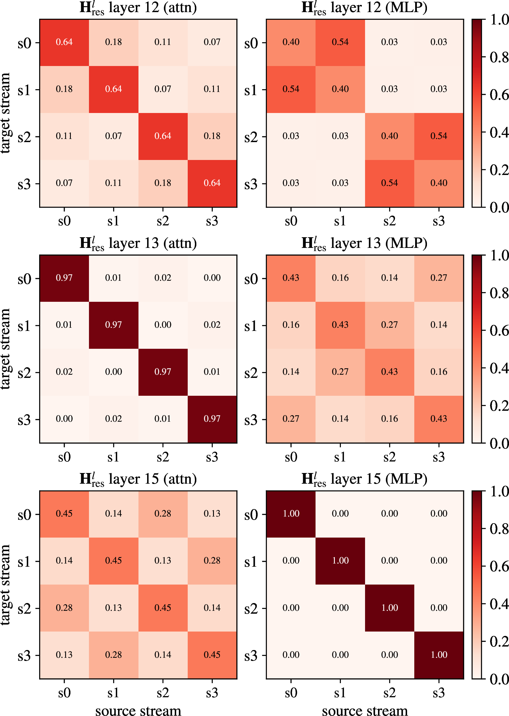
Table 3 shows that increasing \(n\) consistently improves loss, but with diminishing returns. Moving from \(n=2\) to \(n=4\) reduces test loss by 0.02, and moving from \(n=4\) to \(n=8\) gives another 0.02. Then increasing to \(n=16\) gives only a 0.01 improvement, while the number of trainable parameters grows almost four-fold from 12.1 to 43.0.
4.3 Residual mixing and identity preservation↩︎
We next test whether dynamic KromHC uses residual mixing or relies more on its read/write components.
4.3.1 Interpretability↩︎
To gain a deeper understanding of mHC as a PEFT method, we conduct several interpretability experiments, reported in Appendix 17. Most strikingly, \(\mathbf{H}^{l}_{\mathrm{res}}\) was found to shift back to near-identity in later layers, of which Figure 3 contains an example. This pattern is, for instance, visible in layer 13 attention and layer 15 MLP, where the diagonal entries dominate and the off-diagonal entries are close to zero, indicating that the residual streams are propagated almost independently. The finding is in line with earlier interpretability research of mHC for pre-training, where deeper mixing was also found to close to identity in mHC-lite [44]. It suggests that the model learns to suppress cross-stream mixing through \(\mathbf{H}^{l}_{\mathrm{res}}\) rather than exploit it (despite breaking symmetry initially). At the same time, this suppression is not uniform, as other layers show some extent of cross-stream mixing (e.g., layer 12). One hypothesis could be that \(\mathbf{h}^{l}_{\mathrm{pre}}\) and \(\mathbf{h}^{l}_{\mathrm{post}}\) play a more essential role than \(\mathbf{H}^{l}_{\mathrm{res}}\) itself, which we discuss next.
4.3.2 Ablation: residual mixing components↩︎
To further investigate the interpretability findings and to isolate the contribution of each of the three routing objects (\(\mathbf{h}^{l}_{\mathrm{pre}}\), \(\mathbf{H}^{l}_{\mathrm{res}}\), and \(\mathbf{h}^{l}_{\mathrm{post}}\)) and their pairwise interactions, we run ablation experiments. Each routing object in mHC has a distinct role: \(\mathbf{h}^{l}_{\mathrm{pre}}\) selects the branch input from the streams, \(\mathbf{H}^{l}_{\mathrm{res}}\) mixes streams across depth, and \(\mathbf{h}^{l}_{\mathrm{post}}\) writes back to the streams. Ablations are implemented by replacing a component with its identity-preserving neutral form, consistent with the work by [11] (while making sure the diagnostics of Section 4.4 still pass). \(\mathbf{h}^{l}_{\mathrm{pre}}\) is replaced by uniform weights of \(1/n\), \(\mathbf{H}^{l}_{\mathrm{res}}\) by the identity matrix, and \(\mathbf{h}^{l}_{\mathrm{post}}\) by uniform ones. For efficiency, we adapt the code of KromHC such that ablating \(\mathbf{H}^{l}_{\mathrm{res}}\) additionally drops its residual coefficients entirely, so that component’s parameters are removed rather than merely fixed.
We perform six runs with \(n=4\) streams and train for \(3000\) steps. We individually ablate each object and the possible pairs. Table 4 reports the results. The findings indicate that \(\mathbf{h}^{l}_{\mathrm{pre}}\) and \(\mathbf{h}^{l}_{\mathrm{post}}\) are crucial for performance. This is in line with the suggestions of the interpretability experiments (discussed in Section 4.3.1 and Appendix 17).
Notably, these results are in contrast with the findings of [11], where the residual mapping was linked to higher performance gains in pre-training. We hypothesise that this can be linked to a fundamental discrepancy between pre-training and finetuning. In pre-training, representations are learned from scratch and \(\mathbf{H}^{l}_{\mathrm{res}}\) can effectively use stream routing. In contrast, when finetuning, the base model already has rich representation in its residual streams. By imposing to mix residual streams at every layer with normalisation, pre-trained representation may be disrupted. Potentially, keeping \(\mathbf{H}^{l}_{\mathrm{res}}\) as an identity matrix might be key in the use of mHC for finetuning.
| \(\mathbf{H}^{l}_{\mathrm{res}}\) | \(\mathbf{h}^{l}_{\mathrm{pre}}\) | \(\mathbf{h}^{l}_{\mathrm{post}}\) | \(\mathcal{L}_\mathrm{train}\) | \(\Delta\mathcal{L}_\mathrm{train}\) vs mHC | \(\mathcal{L}_\mathrm{test}\) |
|---|---|---|---|---|---|
| ✔ | ✔ | ✔ | 1.38 | — | 1.32 |
| ✔ | ✔ | 1.43 | \(+\)0.05 | 1.36 | |
| ✔ | ✔ | 1.52 | \(+\)0.14 | 1.46 | |
| ✔ | ✔ | 1.50 | \(+\)0.12 | 1.43 | |
| ✔ | 1.52 | \(+\)0.14 | 1.46 | ||
| ✔ | 1.50 | \(+\)0.12 | 1.43 | ||
| ✔ | 2.02 | \(+\)0.64 | 2.00 |
4.5pt
4.3.3 Training with \(\mathbf{H}^{l}_{\mathrm{res}} = \mathbf{I}_n\)↩︎
Since we found that the residual matrix \(\mathbf{H}^{l}_{\mathrm{res}}\) converges to identity in later layers and that the ablation of \(\mathbf{H}^{l}_{\mathrm{res}}\) results in a minimal training loss gap, we run experiments with \(\mathbf{H}^{l}_{\mathrm{res}} = \mathbf{I}_n\). If the trained matrix is (near-)identity regardless, the parameters used to represent it can be removed while cleanly separating two sources of benefit: adding streams (the per-stream read/write gates \(\mathbf{h}^{l}_{\mathrm{pre}}, \mathbf{h}^{l}_{\mathrm{post}}\)) versus learned depth-wise mixing (\(\mathbf{H}^{l}_{\mathrm{res}}\)). Furthermore, to test whether identity preservation is not due to it being a local optimum induced by initialisation, we compared several \(\mathbf{H}^{l}_{\mathrm{res}}\) initialisation schemes, as detailed in Appendix 16.1.
We train KromHC with \(\mathbf{H}^{l}_{\mathrm{res}}\) fixed to identity with the number of streams at \(n \in \{2, 4, 8, 16\}\) for 20000 steps, matching the configuration of 4.2 in every respect except for the \(\mathbf{H}^{l}_{\mathrm{res}} = \mathbf{I}_n\) constraint. Table 5 reports the results.
We see that fixing \(\mathbf{H}^{l}_{\mathrm{res}}=\mathbf{I}_n\) does not hurt performance. Instead, it improves test loss for every expansion rate while removing the residual-mixing parameters. The improvement grows with the number of streams; at \(n=16\), the identity variant reduces test loss from \(1.32\) to \(1.27\) while saving \(\require{physics} \qty{8.39}{\text{M}}\) trainable parameters. This suggests that, in finetuning, the main benefit of dynamic KromHC comes from input-dependent read/write routing through \(\mathbf{h}^{l}_{\mathrm{pre}}\) and \(\mathbf{h}^{l}_{\mathrm{post}}\), rather than from learned depth-wise residual mixing.
Furthermore, these results strengthen the interpretation from the ablation and interpretability studies. Although \(\mathbf{H}^{l}_{\mathrm{res}}\) is central in the original mHC pre-training setting, learning this matrix appears unnecessary, and even harmful, in our frozen-backbone finetuning setup. We therefore use the identity-preserving dynamic KromHC variant in the following experiments unless stated otherwise, and refer to it as mHC\(_\mathrm{identity}\) from here on.
| \(n\) | # params | # params saved | \(\mathcal{L}_\mathrm{train}\) | \(\mathcal{L}_\mathrm{test}\) | \(\Delta\mathcal{L}_\mathrm{test}\) |
|---|---|---|---|---|---|
| 2 | 655 | 262 | 1.42 | 1.36 | -0.01 |
| 4 | 2.36 | 1.05 | 1.39 | 1.33 | -0.02 |
| 8 | 8.91 | 3.15 | 1.37 | 1.31 | -0.02 |
| 16 | 34.6 | 8.39 | 1.33 | 1.27 | -0.05 |
4pt
\begin{table}[b]
3.5pt
| Benchmark | # trainable | BBH | DROP | GSM8K | HellaSwag | MATH | MMLU | PIQA | TriviaQA |
| (Metric) | params | (EM \(\uparrow\)) | (F1 \(\uparrow\)) | (EM \(\uparrow\)) | (N.Acc.\(\uparrow\)) | (EM \(\uparrow\)) | (Acc. \(\uparrow\)) | (Acc. \(\uparrow\)) | (EM \(\uparrow\)) |
| # Shots | – | 3-shot | 3-shot | 8-shot | 10-shot | 4-shot | 5-shot | 0-shot | 5-shot |
| Baseline: OLMo-2 | 0 | 20.73 | 2.22 | 27.60 | 49.58 | 6.14 | 31.41 | 75.52 | 27.20 |
| Prompt tuning | 41.0 | 29.04 | 3.20 | 29.57 | 49.87 | 5.58 | 31.89 | 75.95 | 25.85 |
| (IA)\(^3\) | 328 | 29.30 | 2.56 | 28.73 | 49.38 | 5.74 | 26.29 | 75.19 | 25.59 |
| VeRA | 427 | 27.85 | 2.66 | 29.57 | 49.31 | 5.14 | 29.63 | 74.54 | 25.94 |
| LoRA | 6.03 | 26.66 | 5.41 | 31.39 | 50.06 | 1.50 | 23.73 | 74.70 | 0.06 |
| Layer tuning | 67.1 | 25.19 | 0.43 | 14.86 | 50.26 | 0.44 | 28.94 | 74.92 | 0.04 |
| mHC\(_{\mathrm{identity},n = 2}\) | 656 | 26.23 | 0.59 | 23.28 | 49.62 | 5.42 | 25.69 | 76.01 | 25.69 |
| mHC\(_{\mathrm{identity},n = 4}\) | 2.36 | 26.92 | 0.56 | 25.32 | 49.83 | 5.43 | 25.70 | 75.46 | 27.74 |
| mHC\(_{n = 4}\) | 3.41 | 22.47 | 1.64 | 22.67 | 49.66 | 2.16 | 24.45 | 75.41 | 15.34 |
| mHC\(_{\mathrm{identity}, n = 8}\) | 8.91 | 24.94 | 0.71 | 22.74 | 50.00 | 5.06 | 29.28 | 75.57 | 15.01 |
-0.1in \end{table}
4.4 mHC versus baselines↩︎
Table ¿tbl:tab:benchmark95results95mhc? reports downstream performance on eight benchmark tasks; details are given in Table 1 and Section 3.5. The goal here is to test whether the loss improvements from mHC\(_\mathrm{identity}\) translate to standard evaluation tasks, and how this compares to established PEFT methods.
Comparison to PEFT baselines. No single method dominates the benchmarks. LoRA and VeRA remain strong standalone PEFT baselines, especially on tasks such as DROP and GSM8K, but their performance is uneven over the different tasks. mHC behaves differently: it is not the best method on benchmarks that require heavy reasoning, but the identity-preserving variants have competitive performance on several knowledge and multiple-choice tasks. For example, mHC\(_\mathrm{identity}\) reaches the best PIQA score at \(n=2\) and the best TriviaQA score at \(n=4\).
Effect of identity preservation. The benchmark results also support the conclusion from the experiments where we looked at the loss: the ordinary mHC variant performs worse than its identity-preserving counterpart on most tasks. For instance, fixing \(\mathbf{H}^{l}_{\mathrm{res}}=\mathbf{I}_n\) improves BBH from 22.47 to 26.92, GSM8K from 22.67 to 25.32, MATH from 2.16 to 5.43, and TriviaQA from 15.34 to 27.74 for the same \(n\).
Effect of expansion rate. Surprisingly, increasing \(N\) does not uniformly improve downstream performance. While the loss experiments show a smooth benefit from larger \(N\) (see Table 3 and Table 5), the benchmark table is more task-dependent. For example, \(N=4\) gives the best TriviaQA score, \(N=2\) gives the best PIQA score, and \(N=8\) gives the strongest HellaSwag and MMLU scores.
Takeaway. Overall, mHC as a standalone PEFT method is competitive in some settings but does not consistently outperform established PEFT baselines. The clearest result is instead mechanistic: identity-preserving mHC is substantially better than learned residual mixing, both in loss and in downstream evaluation. This supports our interpretation that, for frozen-backbone finetuning, mHC should preserve the pretrained residual pathway and use capacity mainly for input-dependent read/write routing.
5 Experiments II: mHC combined with other PEFT methods↩︎
We next test whether mHC can complement existing PEFT methods. This is motivated by the fact that mHC modifies residual routing instead of local weight transformations like LoRA en VeRA. It thus may provide benefits that are complementary to methods such as LoRA and VeRA. We evaluate mHC\(_{\mathrm{identity},n=2}\)+VeRA, static mHC\(_{n=16}\)+LoRA\(_{r=8}\), and mHC\(_{\mathrm{identity},n=2}\)+LoRA\(_{r=8}\). Standalone methods are included as references, and LoRA\(_{r=9}\) is included as an approximate parameter-matched comparison for mHC\(_{\mathrm{identity},n=2}\)+LoRA\(_{r=8}\).
1.3pt
| Method | # trainable | BBH | DROP | GSM8K | HellaSwag | MATH | MMLU | PIQA | TriviaQA |
| (Metric) | params | (EM \(\uparrow\)) | (F1 \(\uparrow\)) | (EM \(\uparrow\)) | (N.Acc.\(\uparrow\)) | (EM \(\uparrow\)) | (Acc. \(\uparrow\)) | (Acc. \(\uparrow\)) | (EM \(\uparrow\)) |
| # Shots | – | 3-shot | 3-shot | 8-shot | 10-shot | 4-shot | 5-shot | 0-shot | 5-shot |
| Baseline: OLMo-2 | 0 | 20.73 | 2.22 | 27.60 | 49.58 | 6.14 | 31.41 | 75.52 | 27.20 |
| VeRA | 427 | 27.85 | 2.66 | 29.57 | 49.31 | 5.14 | 29.63 | 74.54 | 25.94 |
| mHC\(_{\mathrm{identity},n = 2}\) | 656 | 26.23 | 0.59 | 23.28 | 49.62 | 5.42 | 25.69 | 76.01 | 25.69 |
| LoRA\(_{r=8}\) | 6.03 | 26.66 | 5.41 | 31.39 | 50.06 | 1.50 | 23.73 | 74.70 | 0.06 |
| LoRA\(_{r=9}\) | 6.78 | 26.66 | 5.30 | 27.98 | 49.30 | 2.62 | 24.95 | 75.03 | 0.03 |
| mHC\(_{\mathrm{identity},n=2}\)+VeRA | 1.08 | 26.08 | 1.45 | 27.29 | 49.49 | 3.18 | 26.71 | 75.41 | 25.13 |
| static mHC\(_{n=16}\)+LoRA\(_{r=8}\) | 6.03 | 27.06 | 4.01 | 23.20 | 49.17 | 2.14 | 24.59 | 75.08 | 0.02 |
| mHC\(_{\mathrm{identity},n=2}\)+LoRA\(_{r=8}\) | 6.68 | 27.74 | 2.73 | 28.51 | 49.37 | 0.82 | 24.38 | 74.86 | 0.62 |
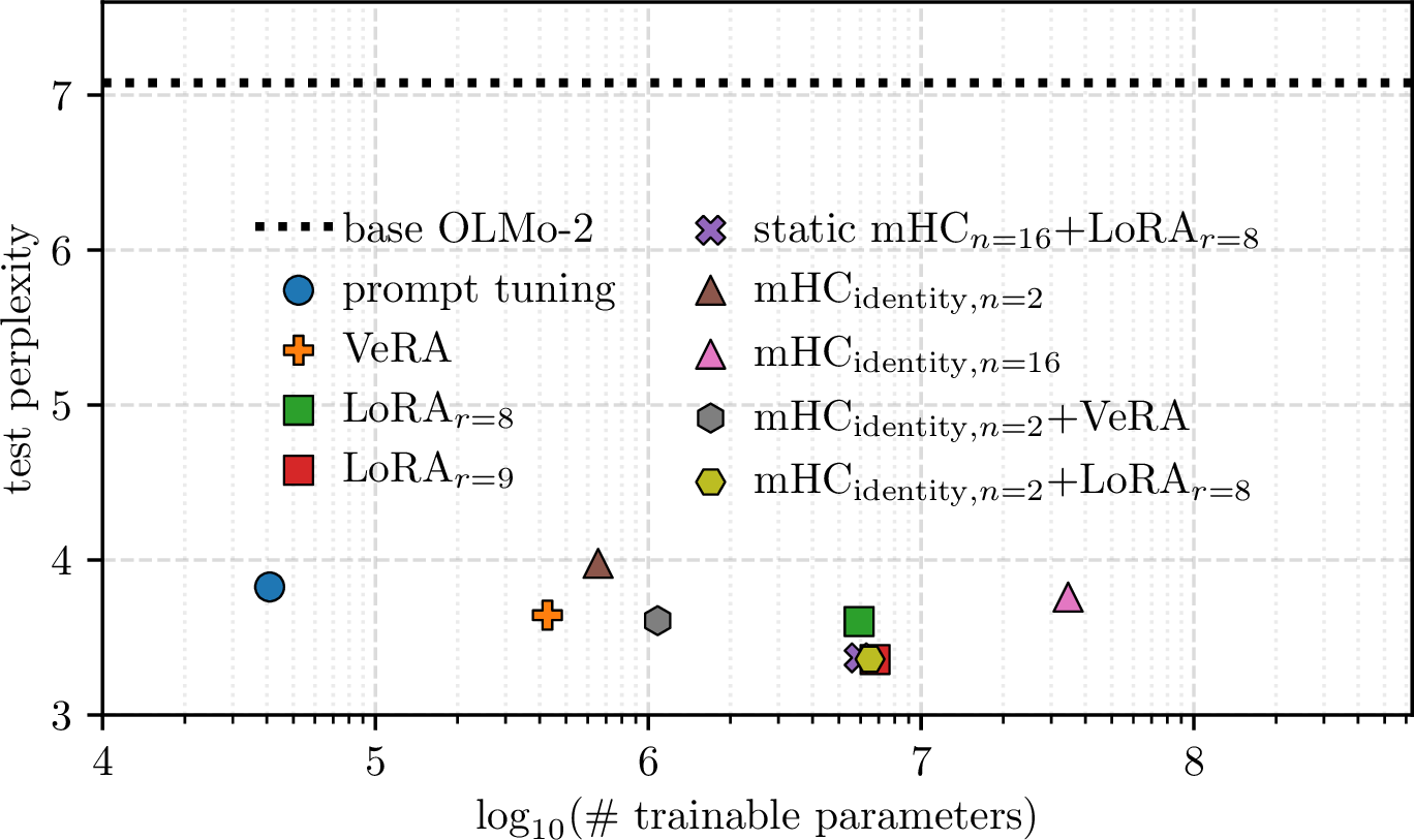
Figure 4 shows that combining mHC with LoRA can improve the trade-off between perplexity and the number of parameters. The combinations yield improved performance for only a small increase in the number of trainable parameters. In particular, static mHC\(_{n=16}\)+LoRA\(_{r=8}\) reduces test loss compared with LoRA\(_{r=8}\) with 1.282 to 1.214, with only 1280 more parameters.
The results on benchmarks can be found in Table ¿tbl:tab:benchmark95results95combinations?. In contrast to the improvement for test perplexity for combinations, the findings across downstream tasks are more mixed. For example, mHC\(_{\mathrm{identity},n=2}\)+LoRA\(_{r=8}\) improves over LoRA\(_{r=8}\) on BBH, MMLU, PIQA, and TriviaQA, but is worse on DROP, GSM8K, HellaSwag, and MATH. Similarly, static mHC\(_{n=16}\)+LoRA\(_{r=8}\) improves over LoRA\(_{r=8}\) on BBH, MMLU, and PIQA, but not on most others. Overall, none of the combinations consistently outperform their standalone methods on all benchmarks. This suggests that the interaction between residual routing and existing PEFT methods might be task-dependent. So, mHC could be useful as a complementary routing mechanism, but benefits and/or drawbacks depends on the task. This finding that mHC and PEFT combinations are not consistently better at this scale motivates the larger-scale comparison in Section 6.
6 Experiments III: mHC with larger models↩︎
| Method | # params | \(\mathcal{L}_\mathrm{train}\) | \(\mathcal{L}_\mathrm{test}\) |
|---|---|---|---|
| OLMo-2-7B | 0 | – | 1.770 |
| mHC\(_{\mathrm{identity}, n=2}\) | 2.62 | 1.143 | 1.095 |
| LoRA\(_{r=2}\) | 2.50 | 1.053 | 1.016 |
| mHC\(_{\mathrm{identity}, n=4}\) | 9.44 | 1.122 | 1.076 |
| LoRA\(_{r=4}\) | 9.99 | 1.023 | 0.995 |
| LoRA\(_{r=14}\) | 35.0 | 1.004 | 0.981 |
| mHC\(_{\mathrm{identity}, n=2}\)+LoRA\(_{r=13}\) | 35.1 | 1.001 | 0.980 |
3.5pt
We train selected adapters on OLMo-2-1124-7B to test whether the main findings transfer to a larger model. We compare mHC\(_\mathrm{identity}\) to LoRA at approximately matched parameter budgets: for mHC the budget is controlled by expansion rate \(n\), for LoRA by rank \(r\) [5]. Matching the parameters isolates both inductive biases and directly compares low-rank weight updates with multi-stream residual routing. All are trained for 20000 steps.
Table 6 shows that the trends for OLMo-2-1B found in previous sections also hold at larger scale. For example, mHC\(_{\mathrm{identity}}\) substantially improves over the frozen OLMo-2-7B baseline in both training and test loss. However, at approximately matched parameter budgets, LoRA achieves a lower train and test loss as a standalone PEFT method: LoRA\(_{r=2}\) outperforms mHC\(_{\mathrm{identity}, n=2}\), and LoRA\(_{r=4}\) outperforms mHC\(_{\mathrm{identity}, n=4}\). This suggests that low-rank weight updates are more effective than residual-stream routing when each is used alone.
The combination result is more promising. Replacing one LoRA rank with mHC parameters improves loss minimally: mHC\(_{\mathrm{identity}, n=2}\)+LoRA\(_{r=13}\) gets a \(\mathcal{L}_\mathrm{test}\) of 0.980 vs.0.981 for LoRA\(_{r=14}\) at nearly equal parameter count. The gain is small, so the result should be interpreted cautiously. Still, it indicates that residual routing does not simply duplicate the effect of LoRA; it is consistent with the idea that mHC and LoRA affect different model parts: LoRA changes local weight transformations and mHC changes how representations are routed through residual streams.
Table ¿tbl:tab:benchmark95results957b? gives a more balanced picture than the loss results alone and shows downstream benchmark results. At nearly matched parameter budget, mHC\(_{\mathrm{identity},n=2}\)+LoRA\(_{r=13}\) improves over LoRA\(_{r=14}\) on 4 out of 8 benchmarks: GSM8K, HellaSwag, PIQA, and TriviaQA, while LoRA is stronger on the others. These results suggest that sometimes one LoRA rank can be replaced by an mHC routing module and give task-dependent improvement on downstream tasks.
1.8pt
| Method | # trainable | BBH | DROP | GSM8K | HellaSwag | MATH | MMLU | PIQA | TriviaQA |
| (Metric) | params | (EM \(\uparrow\)) | (F1 \(\uparrow\)) | (EM \(\uparrow\)) | (Acc. \(\uparrow\)) | (EM \(\uparrow\)) | (Acc. \(\uparrow\)) | (Acc. \(\uparrow\)) | (EM \(\uparrow\)) |
| # Shots | – | 3-shot | 3-shot | 8-shot | 10-shot | 4-shot | 5-shot | 0-shot | 5-shot |
| LoRA\(_{r=14}\) | 35.0 | 47.57 | 6.08 | 58.53 | 60.00 | 5.48 | 59.75 | 79.27 | 0.03 |
| mHC\(_{\mathrm{identity}, n=2}\)+LoRA\(_{r=13}\) | 35.1 | 45.80 | 3.93 | 60.65 | 60.30 | 3.68 | 57.06 | 79.60 | 0.07 |
7 Discussion↩︎
This is the first study to apply mHC in finetuning rather than pre-training. The method trains stably and improves loss with relatively few trainable parameters, showing that residual routing can be used as a PEFT mechanism for frozen Transformers. However, as a standalone method, mHC is generally weaker than established PEFT baselines such as LoRA and VeRA [5], [45], and does not consistently outperform other lightweight baselines across downstream tasks. Nonetheless, this comparison is insightful because mHC adapts a different object than the PEFT baselines considered here. Where LoRA and VeRA modify weight updates and \((\mathrm{IA})^3\) rescales activations, mHC changes how representations are routed through residual streams. Thus, the reported potential of mHC opens residual routing as a separate axis for finetuning.
Identity preservation in finetuning. A central finding is that mHC behaves differently in finetuning than in the pre-training setting for which it was introduced by [10] and [11]. Through routing analysis, we found that learned \(\mathbf{H}^{l}_{\mathrm{res}}\) often moves toward an identity-like structure, i.e.\(\mathbf{H}^{l}_{\mathrm{res}} \approx \mathbf{I}_n\). Accordingly, we find fixing \(\mathbf{H}^{l}_{\mathrm{res}}=\mathbf{I}_n\) actually improves or preserves performance while also reducing the parameter count. This is an essential mechanistic insight: in frozen-backbone finetuning, mHC appears to help mainly through read/write routing, not through learned residual mixing. In other words, the model benefits from changing which residual streams are read from and written to, while keeping the depth-wise residual path close to the pretrained computation. This result is consistent with the broader role of identity residual connections in preserving information flow through deep networks [6], [8].5
mHC as standalone PEFT method. When applied independently as a PEFT method, mHC reduces the loss and shows stable convergence during training, thus indicating its effectiveness. Static mHC variants are extremely parameter-efficient, but dynamic routing performs better due to greater capacity. Among the dynamic variants, KromHC gives the best trade-off in our experiments, consistent with [24]’s goal of reducing the cost of mHC through Kronecker-structured residual matrices. Following the analysis in Section 4, identity-preserving dynamic KromHC (i.e., mHC\(_\mathrm{identity}\)) is our standalone PEFT method of choice.
mHC as complementary PEFT method. Another key finding is that mHC is more promising as a complementary method than as a replacement PEFT method. Standalone mHC does not consistently beat parameter-matched LoRA. When combined with LoRA, however, mHC can improve the training and test loss, even when just adding 1280 parameters: LoRA\(_{r=8}\) gets test loss 1.28 and static mHC\(_{n=16}\)+LoRA\(_{r=8}\) reduces it to 1.21. The benchmark results are more task-specific: adding residual routing helps on some evaluations, but does not lead to uniform improvement. The same pattern appears at 7B scale, where mHC+LoRA gives a small loss improvement and mixed benchmark gains. We hence view the combination results as evidence that residual routing can add something different from simply increasing LoRA rank.
Limitations and future work. Our conclusions are limited by the scope of the experiments: all main results use the OLMo-2 model family and the same Tulu-based finetuning mixture, so the identity-preservation result could depend on architecture or pre-training setup. Due to computational constraints, we also have limited seed and hyperparameter coverage. In addition, we report trainable parameter count, which does not directly represent the cost of deploying the model in practice. Also, dynamic mHC adds routing operations and bookkeeping of residuals streams, to which our implementation is not yet optimised, e.g.by use of custom kernels. A theoretical explanation for why finetuning prefers identity residual mixing also remains open; one hypothesis is that the pretrained residual pathway already contains useful representations. As a result, instead of relearning cross-stream mixing, finetuning benefits more from modulating how to read and write from/to this pathway, as a form of “residual memory.”
Future work should (i) test the above hypothesis across model families, datasets, and modalities, (ii) should develop further (low-level) optimised implementations, and (iii) study more combinations with existing PEFT methods.
8 Conclusion↩︎
This paper proposes mHC as a PEFT method for frozen Transformers. Unlike prior (m)HC work [10], [11], we ask whether the same mechanism can be inserted after pre-training and trained with the backbone fixed. Our results show that this is possible: mHC trains stably, shows lower training loss and test perplexity and opens residual routing as a separate axis for finetuning.
The main finding is that mHC behaves differently in finetuning than in pre-training. Although learned residual mixing is central to the original mHC formulation, our experiments show that finetuning works better with the pretrained residual pathway untouched. Fixing \(\mathbf{H}^{l}_{\mathrm{res}}=\mathbf{I}_n\) improves or preserves performance while reducing the number of trainable parameters, suggesting that the useful capacity comes mainly from read/write routing rather than learned cross-stream residual mixing.
As a standalone PEFT method, mHC does not consistently outperform strong baselines such as LoRA. However, the combination experiments suggest that residual routing can complement LoRA, with improvements in the training loss and task-specific benchmark gains. Thus, mHC should not be viewed as a direct replacement for existing PEFT methods, but as a new way to adapt how pretrained representations move through the model.
Author contributions↩︎
Oldenburg, de Kam, Zuijdam, Eberson, van Zutphen, and de Wildt contributed to an initial stage of the project, supervised by Verhoeven. Oldenburg, de Kam, and Zuijdam led the subsequent stage to further develop the methods. Zuijdam, Eberson, and van Zutphen conducted the embedded interpretability study.
9 Hyperparameters↩︎
This appendix gives more detail on the hyperparameter configurations and choices.
9.1 High-level GPU memory optimisation↩︎
For determining the sequence length where we strike a balance between speed and data usage, we derive Tulu statistics, see Table 7. For the experiments, we used a maximum sequence length of 2048 tokens. This
threshold ensures that we cover more than 99% of examples in allenai/tulu-3-sft-olmo-2-mixture. We applied the same size to our other experiments.
| Type | Statistic | Value |
|---|---|---|
| Dataset | Hugging Face ID | allenai/tulu-3-sft-olmo-2-mixture |
| Tokenizer | Hugging Face ID | allenai/OLMo-2-1B |
| Token length | \(p_{50}\) | 262 |
| Token length | \(p_{75}\) | 470 |
| Token length | \(p_{90}\) | 741 |
| Token length | \(p_{95}\) | 953 |
| Token length | \(p_{99}\) | 1643 |
| Token length | max | 16440 |
| Truncation rate | \(>1024\) tokens | 4.045% |
| Truncation rate | \(>2048\) tokens | 0.540% |
| Truncation rate | \(>4096\) tokens | 0.085% |
For optimising the effective batch size for the finetuning set-up, we tested multiple batch sizes on a single A100 GPU using OLMo-2-0425-1B with LoRA. To get a conservative memory estimate, we fixed the maximum sequence length at 2048 tokens and padded examples to this length during the test. We then increased the batch size while adjusting gradient accumulation to keep the effective batch size constant.
A per-device batch size of 4 with 4 gradient accumulation steps was the largest stable configuration, giving an effective batch size of 16. Larger sizes, such as 8, resulted in CUDA out-of-memory errors under the worst-case (i.e.with padding to 2048 tokens) setting. Thus, we use the 4-4 configuration for all main finetuning runs. For some smaller experiments, we adjusted the batch size of 8 and 2 gradient accumulation steps.
9.2 Hyperparameters of PEFT methods↩︎
All experiments use a Hydra-managed configuration file. The default values are stored in config.yaml; individual runs override only the method, parameter budget, training length, or learning rate when stated explicitly. Table 8 lists the shared training setup, while Tables 9 and 10 list the method-specific settings used for the main
experiments.
| Hyperparameter | Value |
|---|---|
| Seed | 34 |
| Backbone | OLMo-2-0425-1B |
| Precision | bfloat16 |
| Dataset | allenai/tulu-3-sft-olmo-2-mixture |
| Input format | Chat |
| Packing | Enabled |
| Block size | 2048 |
| Train samples | 320000 (equiv.to batch size of 16 for 20000 steps) |
| Validation samples | 2500 |
| Test samples | 2500 |
| Validation/test split seed | 343434 |
| Optimizer | AdamW [33] |
| Scheduler | cosine |
| Warmup ratio | 0.03 |
| Weight decay | 0.0 |
| Max gradient norm | 1.0 |
| Main training length | 20000 steps |
| Short diagnostic runs | 3000 steps |
| Evaluation interval | 2500 steps |
3.5pt
5pt
| Method | Hyperparameter | Value |
|---|---|---|
| LoRA | Rank \(r\) | 8 |
| Alpha | 16 | |
| Dropout | 0.05 | |
| Bias | None | |
| Target modules | q,k,v,o,up,down,gate_proj | |
| Learning rate | 1e-4 | |
| VeRA | Rank \(r\) | 8 |
| Dropout | 0.05 | |
| Projection seed | 343434 | |
| Target modules | q,k,v,o,up,down,gate_proj | |
| Learning rate | 4e-3 | |
| \((\mathrm{IA})^{3}\) | Feedforward modules | up,down,gate_proj |
| Bias | None | |
| Learning rate | 3e-3 | |
| Prompt tuning | Virtual tokens | 20 |
| Initialisation text | None | |
| Learning rate | 1e-2 | |
| Layer tuning | Train last \(N\) layers | 1 |
| Train LM head | False | |
| Train final norm | False | |
| Learning rate | 3e-4 |
3.5pt
4pt
| Method | Hyperparameter | Value |
|---|---|---|
| Static Sinkhorn mHC | Expansion rate \(n\) | 4 unless varied |
| Residual mixer | Sinkhorn | |
| Sinkhorn iterations | 20 | |
| Sinkhorn \(\epsilon\) | 1e-6 | |
| Learning rate | 1e-3 | |
| Static mHC-lite | Expansion rate \(n\) | 4 |
| Residual mixer | Birkhoff–von Neumann mixture | |
| Learning rate | 1e-3 | |
| Static KromHC | Expansion rate \(n\) | 4 |
| Residual mixer | Kronecker factors | |
| Learning rate | 1e-3 | |
| Dynamic Sinkhorn mHC | Expansion rate \(n\) | 4 |
| Residual mixer | Sinkhorn | |
| Sinkhorn iterations | 20 | |
| Sinkhorn \(\epsilon\) | 1e-6 | |
| Learning rate | 1e-4 | |
| Dynamic mHC-lite | Expansion rate \(n\) | 4 |
| Residual mixer | Birkhoff-von Neumann mixture | |
| Learning rate | 1e-4 | |
| Dynamic KromHC | Expansion rate \(n\) | \(\{\num{2}, \num{4}, \num{8}, \num{16}\}\) |
| Residual mixer | Kronecker factors | |
| Learning rate | 1e-3 | |
| mHC\(_\mathrm{identity}\) | Expansion rate \(n\) | \(\{\num{2}, \num{4}, \num{8}, \num{16}\}\) |
| Residual mixer | Fixed identity | |
| Learning rate | 1e-3 |
4pt
| Method | Hyperparameter | Value |
|---|---|---|
| static mHC\(_{n=16}\)+LoRA\(_{r=8}\) | Backbone | OLMo-2-0425-1B |
| KromHC variant | Static KromHC | |
| Expansion rate \(n\) | 16 | |
| \(\mathbf{H}^{l}_{\mathrm{res}}\) | Learned | |
| LoRA rank | 8 | |
| LoRA alpha | 16 | |
| LoRA dropout | 0.05 | |
| Target modules | q,k,v,o,up,down,gate | |
| mHC learning rate | 1e-3 | |
| LoRA learning rate | 1e-4 | |
| Training steps | 20000 | |
| mHC\(_{\mathrm{identity}, n=2}\)+LoRA\(_{r=13}\) | Backbone | OLMo-2-1124-7B |
| mHC variant | Dynamic KromHC | |
| Expansion rate \(n\) | 2 | |
| \(\mathbf{H}^{l}_{\mathrm{res}}\) | Fixed identity | |
| LoRA rank | 13 | |
| LoRA alpha | 16 | |
| LoRA dropout | 0.05 | |
| Target modules | q,k,v,o,up,down,gate | |
| mHC learning rate | 1e-3 | |
| LoRA learning rate | 1e-4 | |
| Training steps | 20000 |
3.5pt
4pt
10 Identity property↩︎
The mHC module should behave like a standard residual connection at initialisation, because pre-trained transformer weights are trained expecting residual connections. An initial behaviour similar to standard residual connections has several benefits. Primarily, it ensures that finetuning starts from OLMo’s optimised pretraining maximum. This prevents using the capacity of mHC to claw back to OLMo-equivalent behaviour from a degraded starting state. Secondly, it follows the identity-mapping principle of residual connections. The added capacity is initially inactive but becomes active during training. It is activated gradually, rather than forcing the network to recover from a disrupted state. Lastly, when mHC is identical to vanilla OLMo at initialisation, any improvement or degradation that is subsequently measured is attributable purely to what mHC learns during training, not to a coincidentally favourable or unfavourable initialisation. This property was tested by checking whether the vanilla OLMo and mHC-wrapped OLMo model’s final logits are sufficiently numerically close. Further, we directly test the residual identity equation by comparing the output of one mHC-wrapped sub-layer against \(x + \mathrm{branch}(x)\). If this holds, the mHC wrapper behaves like a standard residual connection at initialisation.
The routing objects in each mHC module are initialised to preserve this property. \(\mathbf{H}^{l}_{\mathrm{res}}\) should be a doubly stochastic matrix to preserve the mean residual signal, which is done by setting \(\tilde{\mathbf{H}}^{l}_{\mathrm{res}}\) logits to zero and applying Sinkhorn, giving \(\mathbf{H}^{l}_{\mathrm{res}} = \frac{1}{n} \mathbf{11}^T\). \(\mathbf{h}^{l}_{\mathrm{pre}}\) is initialised as the uniform average \(\frac{1}{n}\mathbf{1}\). \(\tilde{\mathbf{h}}^{l}_{\mathrm{post}}\) logits are set to zero, making \(\mathbf{h}^{l}_{\mathrm{post}} = 2\sigma(0) = 1\), thereby writing back the stream output to every stream with weight one.
This property was tested by checking whether the vanilla OLMo and mHC-wrapped OLMo model’s final logits are sufficiently numerically close. Further, we directly test the residual identity equation by comparing the output of one mHC-wrapped sub-layer against \(x + \mathrm{branch}(x)\). If this holds, the mHC wrapper behaves like a standard residual connection at initialisation.
11 Symmetry breaking↩︎
At initialisation, all streams start identically, and the gating matrices start symmetric. Due to this symmetry, the model will not differentiate between streams and exhibits \(S_n\) stream-permutation symmetry. The consequence of this symmetry is that the gradients are also symmetric. After one or multiple update steps, the streams will remain identical, and the model is stuck at this symmetric fixed point. The purpose of multiple streams is therefore defeated since the streams will never diverge and specialise. To break the symmetric fixed point, we implemented a two-stage strategy. First, we introduce noise on the gating matrices. Second, we apply Bernoulli dropout to \(\mathbf{H}^{l}_{\mathrm{res}}\), which adds the advantage of regularisation besides breaking symmetry.
11.1 Two-stage strategy↩︎
For stage 1, at initialisation we add small Gaussian noise (\(\sigma = 10^{-2}\)) to all three learnable gating matrices to perturb the symmetric fixed point of the stream-permutation symmetry, while preserving residual-equivalence within numerical tolerance. The noise on \(\mathbf{H}^{l}_{\mathrm{res}}\) requires no constraint, because Sinkhorn projection guarantees row-stochasticity regardless of input. For \(\mathbf{h}^{l}_{\mathrm{post}}\), the noise introduces only a sub-percent deviation from the target \(\mathbf{h}^{l}_{\mathrm{post}} = 1\). For \(\mathbf{h}^{l}_{\mathrm{pre}}\) we explicitly renormalise after adding noise, to maintain the convex combination property \(\sum_{s=1}^{n} h^{l}_{s,\mathrm{pre}} = 1\). This is crucial for the branch input to equal the embedding when streams are identical at layer 0.
For stage 2, during training we additionally apply Bernoulli logit dropout \((p = 0.1)\) exclusively to \(\mathbf{H}^{l}_{\mathrm{res}}\). Random entries are set to \(-\infty\) before applying the Sinkhorn normalisation. We add a safety check to prevent fully masked rows or columns. This per-forward pass stochastic perturbation directly targets the residual mixing matrix where cross-stream information exchange happens, while Sinkhorn’s row- and column-stochasticity guarantees no magnitude distortion on the residual stream. We deliberately restrict logit dropout to \(\mathbf{H}^{l}_{\mathrm{res}}\) because dropout on \(\mathbf{h}^{l}_{\mathrm{pre}}\) would break the convex combination property, and dropout on \(\mathbf{h}^{l}_{\mathrm{post}}\) would require similar normalisation to preserve the residual-equivalent initialisation condition. Both effects would complicate the analysis without providing additional symmetry-breaking benefits, since initialisation noise alone already breaks symmetry for these mappings. During inference, dropout is not applied.
Altough the symmetry-breaking perturbations technically break exact residual-equivalence between the mHC-wrapped model and vanilla OLMo, this is not a concern in practice. We verify empirically that the resulting deviation stays within a tight numerical
tolerance. The final logits of the wrapped and vanilla models remain close, and the single-sublayer output stays within roughly \(1\%\) of \(x+\mathrm{branch}(x)\). A deviation of this
magnitude is negligible relative to the scale of the hidden states and is comparable to the rounding error already introduced by bf16 precision. The model, therefore, still starts from a point that is, for all practical purposes, OLMo’s
pretrained minimum, i.e.the loss at initialisation is effectively unchanged, gradients remain small, and no early instability is introduced. The perturbation is a necessary trade-off. It sacrifices exact equality to allow streams to differentiate.
12 Sinkhorn normalisation↩︎
Sinkhorn normalisation maps unconstrained residual-routing logits to an approximately doubly stochastic matrix. Given logits \(\tilde{\mathbf{H}} \in \mathbb{R}^{n \times n}\), we first form a positive matrix \[\mathbf{M}^{(0)} = \exp\left(\tilde{\mathbf{H}}\right).\] The Sinkhorn-Knopp procedure then alternates row and column normalisation as follows [16]: \[\mathbf{M}^{(t + 1/2)}_{ij} = \frac{ \mathbf{M}^{(t)}_{ij} }{ \sum_{k=1}^{n}\mathbf{M}^{(t)}_{ik} }, \qquad \mathbf{M}^{(t+1)}_{ij} = \frac{ \mathbf{M}^{(t+1/2)}_{ij} }{ \sum_{k=1}^{n}\mathbf{M}^{(t+1/2)}_{kj} }.\] For positive matrices, this procedure converges to a doubly stochastic matrix under standard conditions [16]. In practice, mHC uses a finite number of iterations. Our implementation performs the normalisation in log space for numerical stability and uses 20 iterations, matching the original mHC configuration by [11]. Lastly, recent work by [15] suggests that this iterative projection can be avoided through an exact doubly stochastic reparameterisation.
13 PEFT baselines↩︎
This appendix primarily supplements Section 2.4. In addition to LoRA as a PEFT baseline, we compare against VeRA, \((\mathrm{IA})^3\), prompt- and layer tuning. These baselines cover different adaptation mechanisms: VeRA is an ultra-light LoRA-style weight adaptation method, \((\mathrm{IA})^3\) rescales intermediate activations, prompt tuning learns input-side soft prompts, and layer tuning updates only a specific subset of layers are updated. We explain them below in a bit more detail.
VeRA further reduces the trainable parameter count of LoRA-style adaptation [45]. Instead of learning the low-rank matrices \(\mathbf{A}\) and \(\mathbf{B}\), VeRA keeps random low-rank matrices frozen and shared across layers, and only trains small scaling vectors. For an adapted matrix with output dimension \(d\) and rank \(r\), this gives approximately \(d + r\) trainable parameters per adapted layer, compared to \(r(d+k)\) for LoRA. VeRA is therefore a useful lightweight PEFT baseline for mHC.
(IA)3 learns task-specific vectors that rescale intermediate activations in attention and feed-forward layers [46]. It is from PEFT family that adapts activations rather than weight matrices. This is highly parameter-efficient because the learned parameters are element-wise scaling vectors rather than matrices or low-rank updates.
Layer tuning is a simple partial-finetuning baseline [3]. Instead of adding new parameters, it keeps most of the pre-trained model frozen and updates only a small number of existing layers. In our case, this means finetuning the final Transformer layer. This baseline is useful because it tests whether updating the highest-level representations of the backbone is sufficient for adaptation.
Prompt tuning adapts a frozen language model by learning a small set of continuous prompt embeddings that are prepended to the input [47]. The backbone remains frozen, and only these soft prompt vectors are updated. For \(M\) virtual tokens and hidden dimension \(d\), prompt tuning adds \(Md\) trainable parameters. Unlike LoRA, DoRA, and \((\mathrm{IA})^{3}\), prompt tuning does not modify internal weights or activations directly; it changes the input context seen by the model.
Together, these methods provide baselines that act on different parts of the model. LoRA and VeRA adapt selected weight matrices, \((\mathrm{IA})^{3}\) rescales intermediate activations, layer tuning updates a small subset of existing layers, and prompt tuning learns additional input embeddings. mHC targets a different mechanism: it trains how representations are routed through residual streams across depth. This makes mHC a natural standalone PEFT candidate and a possible complement to existing PEFT methods.
14 Data stratification↩︎
To reduce computational cost even further, while maintaining the structure of the original mixed dataset, we constructed a fixed stratified subset before training. The cutoff of 20000 samples was chosen because the training curves for LoRA showed clear signs of approaching stagnation, as shown in Figures 5 (a) and 5 (b). Although the plots suggest that the true plateau may occur closer to 30000-40000 steps, the other methods contain fewer trainable parameters, from which we assume they converge more quickly. We thus choose 20000 as our cut-off, also to save compute.
For mixture datasets, the raw dataset is passed through a proportional sampling function with a maximum sample budget, set through stratify_max_samples and defaulting to 20000 samples. The sampling is performed with respect to a
configurable source_column, which defaults to “source.”
The procedure first counts the number of examples belonging to each source in the full dataset. For a target subset size \(n\), it then assigns each source a sampling budget proportional to its original frequency: \(n_s = \lfloor n \cdot \frac{N_s}{N} \rfloor\), where \(N_s\) is the number of examples from source \(s\), and \(N\) is the total dataset size. The remaining samples are distributed to the sources with the largest fractional remainders. Finally, examples are randomly sampled without replacement from each source using a fixed seed, and the selected indices are shuffled. This produces a reduced dataset with approximately the same source distribution as the original dataset.
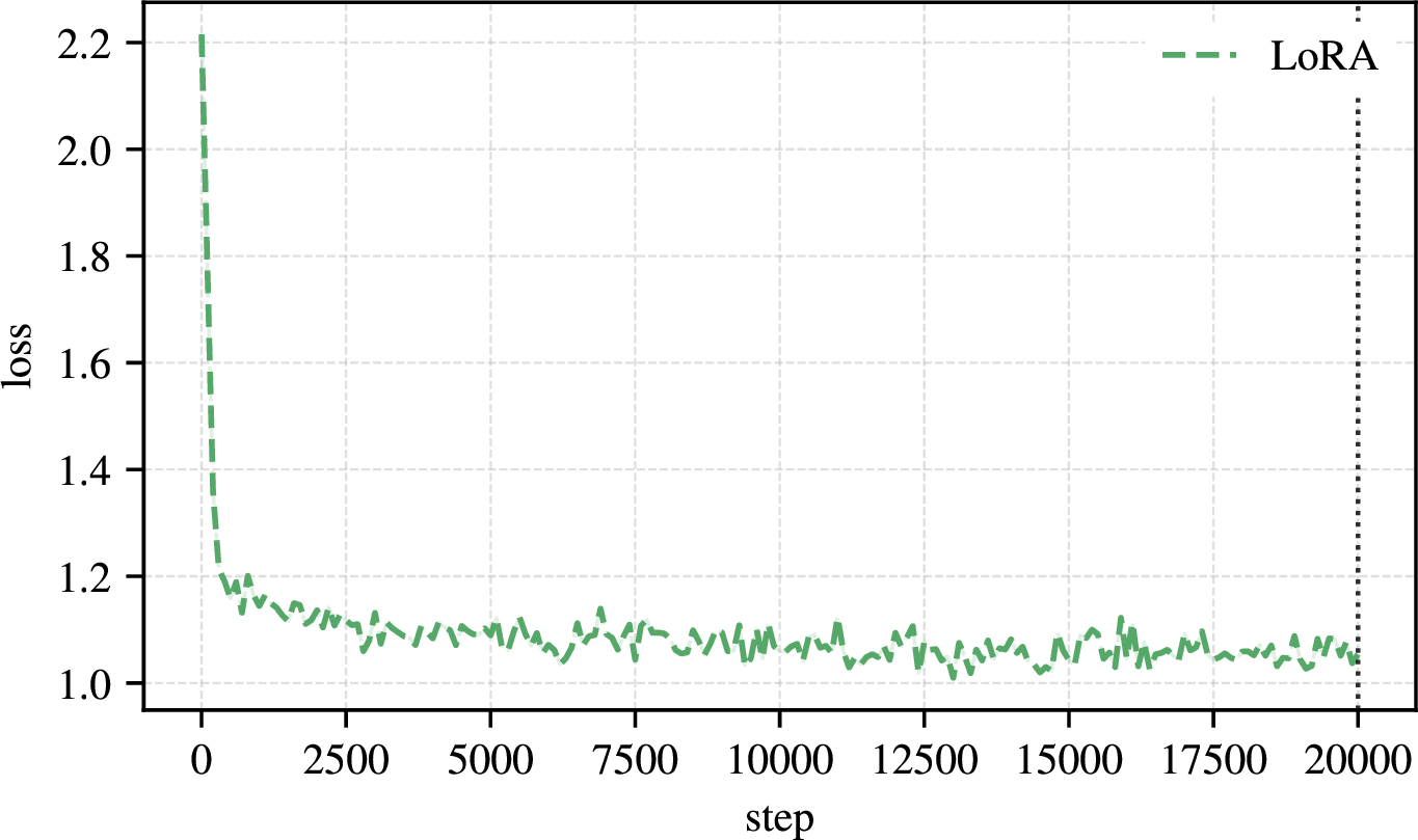
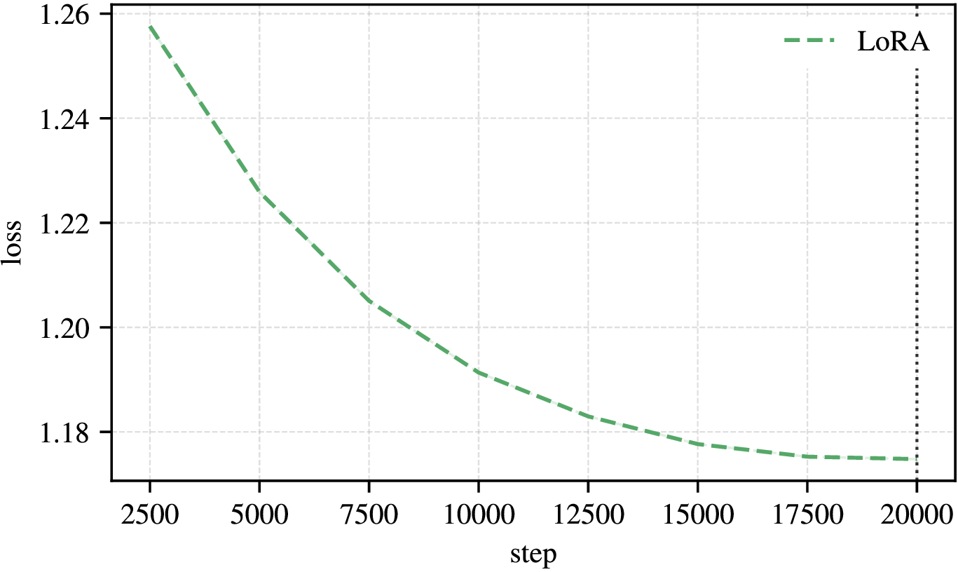
Figure 5: (a): \(\mathcal{L}_\mathrm{train}\) for LoRA on OLMo-2-1B. (b): corresponding \(\mathcal{L}_\mathrm{validation}\).. a — Train loss for LoRA at 20k steps, b — Validation loss for LoRA at 20k steps
15 Downstream benchmarking framework↩︎
To test downstream capabilities of mHC against standard PEFT baselines, all experiments are evaluated on benchmarks from the lm-evaluation-harness from [42]. Every model configuration, as well as the untrained OLMo-2-1B model, is evaluated on the same benchmarks as the paper from [11].
To ensure optimal hardware utilisation on the Snellius HPC cluster, dynamic memory profiling is used via an automatic batching architecture (batch_size = auto). The framework scales the hardware processing threshold to the maximum VRAM
capacity of the process it is currently in, to ensure the fastest possible evaluation, without the risk of an OOM error.
As described in Table ¿tbl:tab:benchmark95details?, the evaluation suite adapted from [11] spanse a diverse range of capabilities, from physical intuition and commonsense reasoning, to tasks such as multi-step logic and advance mathematical problems. This diverse layout ensures a robust assessment of each finetuning method.
\begin{table}[H]
3.5pt
| Benchmark | Context Type | X-Shot Configuration | Evaluation Target | Task Metric |
|---|---|---|---|---|
| PIQA | Physical Intuition | 0-Shot | Cloze Context Matching | Normalised Accuracy |
| HellaSwag | Commonsense Reasoning | 10-Shot | Adversarial Context Completion | Normalised Accuracy |
| MMLU | Multi-discipline Knowledge | 5-Shot | Academic Multiple-Choice | Accuracy |
| BBH | Complex Logic | 3-Shot | Algorithmic Multi-Step Parsing | Exact Match |
| GSM8K | Math Word Problems | 8-Shot | Auto-regressive CoT Generation | Exact Match |
| DROP | Discrete Reading Comp. | 3-Shot | Numerical Macro-Operation | F1-Score |
| MATH | Advanced Mathematics | 4-Shot | Symbolic Math Free-Response | Exact Match |
| TriviaQA | Factoid Knowledge | 5-Shot | Open-Ended Fact Retrieval | Exact Match |
-0.1in \end{table}
16 Ablations and additional experiments↩︎
This appendix discusses ablations of the \(\mathbf{H}^{l}_{\mathrm{res}}\) initialisation, learning rate, and mHC readout.
16.1 Ablation: initialisation of \(\mathbf{H}^{l}_{\mathrm{res}}\)↩︎
[10] initialise \(\mathbf{H}^{l}_{\mathrm{res}}\) as an identity matrix, while [11] do not specify how it is initialised. We therefore set \(\mathbf{H}^{l}_{\mathrm{res}} = \mathbf{I}_n\) at the start, up to numerical a numerical precision of 1e-4 due to noise added for symmetry breaking. We observed in some initial tests that \(\mathbf{H}^{l}_{\mathrm{res}}\) initially diverges from the identity matrix, but quickly moves back to it. This raised the question whether identity is genuinely a preferred solution to model returns to, or merely a local
optimum induced by initialisation.
As discussed in Section 10, we initialise mHC so that the wrapped model starts from the same function as the original OLMo model. Because each tested \(\mathbf{H}^{l}_{\mathrm{res}}\) is row-stochastic, it maps identical streams back to the same streams. Together with unit write-out weights, this means that the wrapped model is initially equivalent to the frozen backbone.
We test whether the choice of \(\mathbf{H}^{l}_{\mathrm{res}}\) initialisation matters after training. For \(n=4\), we compare four initialisations for 3000 steps: identity, uniform, permutation, and noise, where uniform initialisation uses a uniform doubly stochastic matrix, permutation initialisation swaps streams, and noise initialisation starts from the identity and adds bounded off-diagonal mass. We find that the choice of initialisation has little effect on the final result. For all four, training converges to similar losses, and the learned residual mixers move back toward an identity-like structure. This supports the interpretation that, in this finetuning setting, learned cross-stream residual mixing is not the main source of performance. Instead, the model tends to preserve the pretrained residual pathway even when \(\mathbf{H}^{l}_{\mathrm{res}}\) is initialised away from the identity.
16.2 Ablation: learning rate↩︎
We performed hyperparameter tuning to obtain a suitable learning rate (LR) for mHC. Too high an LR can destabilise the warm-start by pushing the dynamic routing terms away from their identity-equivalent initialisation, whereas too low an LR can leave
them near it. All experiments use a cosine LR schedule with fixed \(3\%\) warmup. We sweep LR \(\in\{\texttt{1e-3}, \texttt{5e-4}, \texttt{1e-4}, \texttt{5e-5} \}\) and train dynamic KromHC
with \(n=4\) for \(3000\) steps. We cap the sweep at 1e-3 deliberately. Beyond preserving consistency with the high end of typical PEFT learning rates, larger rates risk
perturbing the identity-equivalent initialisation before the model has adapted, undermining the warm-start property that motivates the manifold constraint. We therefore treat this sweep as selecting a stable operating point for the subsequent
experiments rather than as a search for a globally optimal LR.
We observe an upward trend when increasing the LR from 5e-5 to 1e-3, though the increase progressively diminishes. An LR of 1e-3 achieved the best test loss while retaining stable warm-started training, and this LR
is carried into the longer main experiments.
16.3 Ablation: readout↩︎
During the experiments we found that the final MLP layer was completely uniform, as in Figure 3, caused by the mean pool at the end of the static Sinkhorn mHC module. To test whether this was of any influence, we tested substituting this mean readout with a softmax. Surprisingly, we found that after after 3000 steps, the final \(\mathbf{H}^{l}_{\mathrm{res}}\) was not uniform anymore, though when we continued training to 20000 steps, the matrix returned back to uniform. Accordingly, after 20000 we found little difference in performance.
17 Interpretability experiments↩︎
Recent work on (m)HC showed that residual mixing often remains close to identity in pre-training and that signal and interpretable features concentrate in a dominant stream [44]. A comparable dominance pattern was observed at the causal level, where certain streams exerted significant influence on model output while representationally similar streams remained largely passive [48]. This raises the question whether our mHC implementation for fine-tuning shows the same patterns and if this could be linked to limited effectiveness of mHC as a PEFT method.
To gain a deeper understanding of the inner workings of mHC for fine-tuning, several experiments have been employed. First, to examine the extent to which streams dominate one another, we apply two methods. With per-stream logit lens we investigate the confidence and differences in the prediction over layers per stream. Moreover, since representational similarity between streams has been shown to not necessarily reflect their functional or causal role [48], we complement our logit lens and weight visualisation with stream ablation. Stream ablation causally verifies the effect of each stream for different language tasks (subject/verb, country/capital, IOI, phrase completion). Second, we examine the routing over layers by applying linear Centered Kernel Alignment (CKA). Accordingly, we visualise \(\mathbf{H}^{l}_{\mathrm{res}}\) for selected layer pairs, focusing on layers flagged by the CKA analysis.
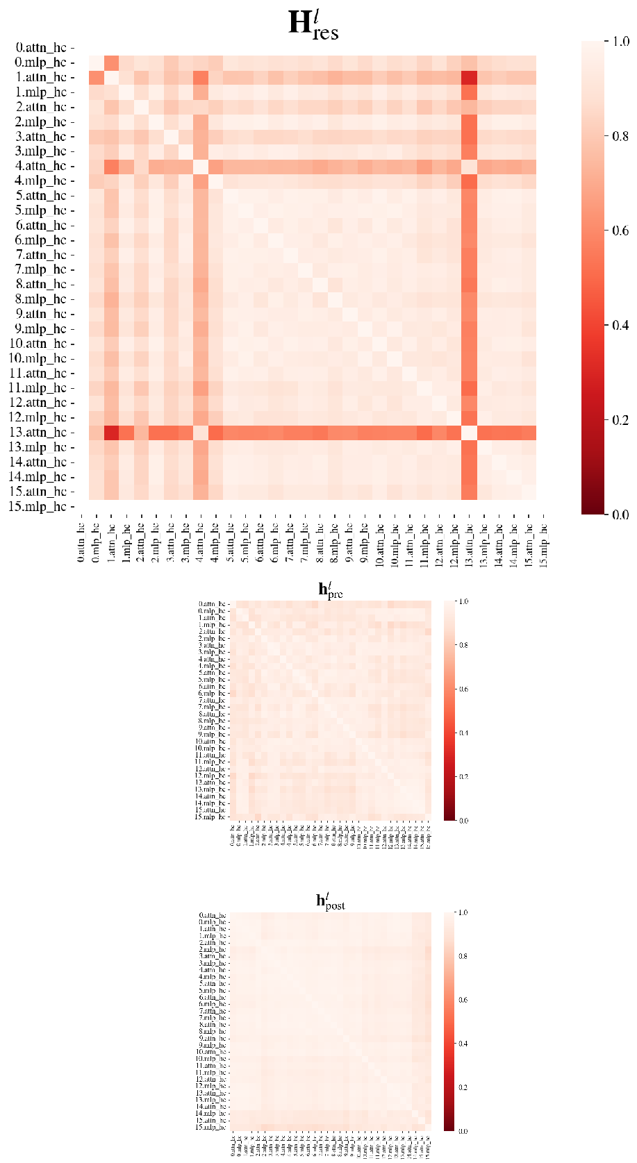



Figure 8: Each panel shows the top-1 predicted token at each layer and position for one KromHC stream. For high-confidence completions, KromHC routing does not induce stream specialisation..
Our results can be found in Figures 6, 7, and 8. Firstly, routing has been found to differ by layer, where most differences can be found in layer 4 and 13. After visualising the weights in these interesting layers from CKA (see Figure 3), it could be concluded that later layers (specifically layer 13) show a shift back to near-identity. Moreover, some layers mix across all streams while others almost entirely refrain. The CKA findings highlight that pre-layer hidden representations are more differentiated across layers, whereas the post-layer representations are substantially more similar. Based on the observed CKA patterns, we hypothesise that \(\mathbf{h}^{l}_{\mathrm{pre}}\) might play a more significant role in layer-wise representation learning, as it exhibit greater representational diversity than the corresponding \(\mathbf{h}^{l}_{\mathrm{post}}\). Secondly, regarding stream specialisation, there is limited evidence of a dominant stream. The stream specialisation patterns are indicated to be prompt-dependent, with its level varying by task. However, since prior work did not focus upon task or prompt types, it remains unclear whether this prompt-dependence is specific to fine-tuning or a pattern that has simply not yet been examined in pre-training.
18 Earlier reported findings on stability for HC and mHC↩︎
The propagation instability of Hyper-Connections have been shown by [11]. This can be seen in Figure 9.
![Figure 9: Propagation Instability of HC. This figure illustrates the propagation dynamics of (a) the single-layer mapping of \mathbf{H}^{l}_{\mathrm{res}}, here denoted as \mathcal{H}^{\mathrm{res}}_l, and (b) the composite mapping \prod_{i=1}^{L-l}\mathbf{H}^{l}_{\mathrm{res}}, here denoted as \prod_{i=1}^{L-l}\mathcal{H}_{L-i}^{\mathrm{res}}, within the 27B model. The layer index l (x-axis) unrolls each standard Transformer block into two independent layers (Attention and FFN). The Amax Gain Magnitude (y-axis) is calculated as the maximum absolute row sum (for the forward signal) and column sum (for the backward gradient), averaged over all tokens in a selected sequence [11]](/article/2607.18130/images/27b_forward_backward_gain.png "fig:")
On the other hand, mHC has been found to improve stability in terms of both loss and gradient norm. This can be seen in Figure 10.
![Figure 10: Training Stability of mHC. This figure illustrates (a) the absolute training loss gap of mHC and HC relative to the baseline, and (b) the gradient norm of the three methods. All experiments utilise the 27B model. The results demonstrate that mHC exhibits improved stability in terms of both loss and gradient norm [11]](/article/2607.18130/images/27b_loss_grad_all.png "fig:")
References↩︎
The module and codebase are available on GitHub: https://github.com/valentijn7/mHC_PEFT.git↩︎
Both the 1B- and 7B-model are downloadable through Hugging Face, via https://huggingface.co/allenai/OLMo-2-0425-1B and https://huggingface.co/allenai/OLMo-2-1124-7B, respectively.↩︎
Public codebase for mHC-lite: https://github.com/FFTYYY/mhc-lite; and for KromHC: https://github.com/wz1119/KromHC.↩︎
Emissions were estimated using CodeCarbon [30]; the estimated carbon intensity of the Netherlands was 143 \(\mathrm{g\,CO_2eq\,kWh^{-1}}\) in May 2026 [31].↩︎
It must be noted that this differs from another well-known phenomenon in finetuning: catastrophic forgetting [2]. With the backbone frozen, the issue is not overwriting pretrained weights, but that learned residual mixing can change how pretrained representations propagate through the model.↩︎