time-inconsistent stochastic control, reinforcement learning, exploratory equilibrium HJB equation, entropy regularization, Volterra operator, feedback cycles, statistical conditioning, Mittag–Leffler function

1 Introduction↩︎

Entropy regularization replaces a point action by a relaxed policy and turns policy improvement into a Gibbs map. In continuous-time reinforcement learning (RL), this gives a smooth Hamiltonian and a tractable policy iteration. Convergence results for time-consistent exploratory HJB equations include [1]–[4]. Entropy annealing and robustness have also been studied for time-consistent continuous-time control [5], [6].

For a time-inconsistent objective, a policy chosen at \((t,x)\) need not remain optimal at a later time. One instead seeks an equilibrium among temporal selves, described by an extended HJB system [7]–[11]. That system is nonlocal: the policy at time \(t\) depends on a diagonal derivative of an auxiliary value function whose reference variables are frozen at \((t,x)\).

Huang, Yu, and Zhang [12] recently proposed an exploratory equilibrium HJB (EEHJB) system for a broad class of these problems, proved fixed-temperature convergence of policy iteration, and constructed a classical solution. A related vanishing-entropy result obtains unregularized equilibria from subsequential EEHJB limits [13]. These works address well-posedness, fixed-model policy iteration, and the zero-temperature limit, but not how learned-model or policy-evaluation errors are amplified as the temperature falls. A fixed-temperature iteration can converge quickly while its equilibrium is poorly conditioned.

Our analysis is self-contained relative to that well-posedness theory. We state the fixed-point system and its data hypotheses in [sec:model] 2 3, construct the mild evaluation map and local equilibrium branch directly, and solve the explicit models separately.

Adjacent perturbation theory covers time-consistent relaxed control [14] and equilibrium-induced values for time-inconsistent stopping [15], [16]. Nonlocal equilibrium HJB equations, equilibrium dynamic programming, and related BSDE representations are studied in [17], [18]. Relaxed equilibria and sample-based learning for time-inconsistent control and decision problems appear in [19]–[22]. None of these results gives a temperature-explicit derivative for a continuous-time exploratory control equilibrium and propagates it through a model estimator.

The organizing point is that low-temperature conditioning is governed not only by the local \(1/\tau\) Gibbs factor, but also by the topology and smoothing of causal returns. A future policy changes the continuation score of every earlier self. In discrete time this derivative is strictly triangular. In continuous time it becomes a backward Volterra operator with infinitely many nonzero causal powers. The series converges for each \(\tau>0\), but its norm may grow exponentially as \(\tau\downarrow0\).

Treating future decision nodes as agents with logit responses goes back to agent quantal response equilibrium in extensive-form games [23]. Static graph QRE can also exhibit Ising-type phase changes [24]. The analogy here is limited: temporal selves form a continuum coupled by a controlled diffusion, and the directed graph describes a causal derivative rather than equilibrium multiplicity.

Let \(\alpha\) denote the smoothing order of the causal kernel. The equilibrium derivative is bounded by \(C\tau^{-1}E_\alpha(\kappa T^\alpha/\tau)\). If the forcing and return kernel preserve an aligned sign, the lower bound has the same small-temperature exponent. Without that sign condition, negative feedback may damp the response.

The block form shows where repeated amplification enters. On a directed acyclic graph, the Neumann series stops at the longest path. Under aligned forcing, a positive \(q\)-cycle with total smoothing order \(\beta\) contributes the lower factor \(E_\beta(C/\tau^q)\) and forces divergence below the scale \((\log n)^{-\beta/q}\). When the corresponding one-step upper bound matches the cycle return, this scale is the linear-response boundary.

To connect conditioning with estimation, we treat a finite-dimensional coefficient family at fixed \(\tau>0\). The mild EEHJB evaluation map is \(C^2\), its causal derivative is invertible, and the resulting equilibrium branch satisfies a function-valued delta method. The parabolic argument gives the general upper scale \(e^{C/\tau^2}\); whether a state-dependent model attains this rate remains open.

Two exact models show what the causal rates mean. In a bounded uniformly elliptic diffusion of arbitrary finite dimension, the tied-policy response is \[\frac{v}{\tau}\exp\left\{\left(-\nu I+\frac{v}{\tau} K\right)(T-t)\right\}.\] For \(K\ge0\), a graph of longest path \(L\) has susceptibility \(\Theta(\tau^{-(L+1)})\), while a positive cycle produces an \(e^{C/\tau}\) factor along a Perron direction. The model also has a nonlinear counterpart: exponentially small signals vanish on a DAG, whereas cooperative feedback selects extreme actions under the positive-row-sum, support, and short-horizon conditions of 5. In the affine model, root-\(n\) reward noise has the exact critical temperature \[\tau_n^\star=\frac{\beta T}{W(\beta T\sqrt n)} \sim\frac{2\beta T}{\log n}.\] Here \(W\) denotes the principal real branch of the Lambert \(W\) function. At this scale the initial policy has a nondegenerate random limit although every fixed later policy converges to the reference mixture.

Time discretization retains this graph dependence. Along a cyclic Perron mode, a uniform \(N\)-step rule has vanishing relative error exactly when \(N\tau^2\to\infty\). For a fixed DAG, \(N\to\infty\) suffices without coupling \(N\) to \(\tau\). The general stability and delta-method results keep \(\tau>0\) fixed; joint small-temperature limits are stated only when an explicit bound or exact model supports them.

The paper follows this causal chain. 2 derives the Gibbs fixed point from infinitesimal spikes. 3 proves the abstract resolvent and graph dichotomy. 4 establishes EEHJB stability and the fixed-temperature delta method. 5 realizes the sharp path–cycle and nonlinear statistical transitions, and 6 closes with discretization and reproducible numerical illustrations.

2 Time-inconsistent relaxed control and the EEHJB score map↩︎

Fix a horizon \(T>0\), state dimension \(d\), and a compact metric action space \(\mathsf A\) equipped with a reference probability measure \(\mu\) of full support. A Markov relaxed policy is a kernel \(\pi(t,x,da)\) absolutely continuous with respect to \(\mu\). Put \[\bar b^\pi(t,x)=\int_\mathsf Ab(t,x,a)\pi(t,x,da), \qquad \bar r_{\tau,y}^\pi(t,x)=\int_\mathsf Ar(\tau,y,t,x,a)\pi(t,x,da).\] Finite action spaces are included: if \(\mu\) gives positive mass to each action, every policy has a density with respect to \(\mu\), and the integrals and relative entropy below are finite sums. For a known, uncontrolled diffusion matrix \(\sigma(t,x)\), the exploratory state is \[\label{eq:state-sde} dX_s^\pi=\bar b^\pi(s,X_s^\pi)\,ds+\sigma(s,X_s^\pi)\,dW_s, \qquad X_t^\pi=x.\tag{1}\] The self whose reference time-state is \((\tau,y)\) evaluates a continuation from \((t,x)\) by \[\begin{align} V^\pi(\tau,t,y,x) :=\mathbb{E}_{t,x}\bigg[&\int_t^T \Big\{r(\tau,y,s,X_s^\pi,A_s) -\tau_e\log\frac{d\pi(s,X_s^\pi)}{d\mu}(A_s)\Big\}\,ds\notag\\ &+F(\tau,y,X_T^\pi)\bigg]. \label{eq:aux-value} \end{align}\tag{2}\] Here, conditionally on the state, \(A_s\) has distribution \(\pi(s,X_s^\pi,\cdot)\). We write the entropy temperature as \(\tau_e>0\) temporarily to distinguish it from the reference-time variable; from 3 onward it is denoted simply by \(\tau\). Nonexponential discounting can be absorbed into \(r\).

The policy-evaluation equation for a fixed admissible \(\pi\) is the family of linear parabolic PDEs \[\begin{align} \partial_tV^\pi+\tfrac12\operatorname{tr} (\sigma\sigma^\top D^2_xV^\pi) +\bar b^\pi\cdot D_xV^\pi+\bar r_{\tau,y}^\pi -\tau_e\operatorname{KL}(\pi(t,x)\Vert\mu)&=0, \label{eq:policy-evaluation-pde}\\ V^\pi(\tau,T,y,x)&=F(\tau,y,x). \notag \end{align}\tag{3}\] The variables \((\tau,y)\) are frozen parameters in this PDE. The acting self at \((t,x)\) sets \((\tau,y)=(t,x)\) but uses the flow-state partial derivative \(D_xV^\pi(t,t,x,x)\), not the total derivative of the diagonal map. Its action score is \[\label{eq:score-map} Q^\pi(t,x,a)=b(t,x,a)\cdot D_xV^\pi(t,t,x,x) +r(t,x,t,x,a).\tag{4}\] The Gibbs variational identity gives the unique pointwise best response \[\label{eq:gibbs-map} \mathcal{G}_{\tau_e}(q)(da) =\frac{\exp(q(a)/\tau_e)\mu(da)}{\int_\mathsf A\exp(q(a')/\tau_e)\mu(da')}.\tag{5}\] Define the best-response operator \[\label{eq:equilibrium-fixed-point} \mathcal{T}_{\tau_e,M}(\pi):=\mathcal{G}_{\tau_e}(\mathcal{Q}_M(\pi)), \qquad M=(b,r,F).\tag{6}\] A regularized Markov equilibrium is a fixed point \(\pi^\star=\mathcal{T}_{\tau_e,M}(\pi^\star)\); when it is unique we write \(\Phi_{\tau_e}(M)=\pi^\star\). Here \(\mathcal{Q}_M\) means: solve 3 and form 4 . This is a compact score-map representation of the EEHJB system. The stability section adds a terminal statistic and a nonlinear function \(G\) and states that extended system explicitly.

The next result anchors this fixed-point formulation in the infinitesimal-spike equilibrium criterion. Its local hypotheses justify the first-order spike limit; the conclusion identifies the Gibbs fixed point as exactly the no-profitable-spike condition.

This equivalence concerns the local equilibrium criterion defined by infinitesimal spikes. It does not assert precommitment optimality or the strong finite-spike equilibrium property.

A perturbation of \(\pi(s,\cdot)\) at \(s>t\) changes \(V^\pi(t,t,\cdot,\cdot)\), hence the score and policy at \(t\). Causality prevents a policy perturbation at an earlier time from changing a later score. Thus \(D_\pi\mathcal{Q}_M\) is a backward Volterra operator.

3 The causal Volterra resolvent↩︎

We first separate the causal argument from the PDE estimates. Let \(X\) and \(Y\) be Banach spaces for policy tangents and centered action scores at one time, respectively, and put \(\mathcal{X}=C([0,T];X)\) and \(\mathcal{Y}=C([0,T];Y)\) with supremum norms. In finite actions, \(X\) is the product of simplex tangent spaces with the \(\ell^1\) norm and \(Y\) carries the oscillation norm. For a signed measure \(\nu\), our total variation convention is \(\left\lVert \nu\right\rVert_{\rm TV}=|\nu|(\mathsf A)\), so the distance between two probability measures is at most two. Let \(\mathsf H\) be a Banach space of primitive model directions.

For \(\alpha>0\), define the right-sided Riemann–Liouville integral \[\label{eq:fractional-integral} (I_{T-}^\alpha f)(t) :=\frac{1}{\Gamma(\alpha)}\int_t^T(s-t)^{\alpha-1}f(s)\,ds.\tag{9}\] We use the convention \(I_{T-}^0=\mathrm{Id}\). The fractional integrals satisfy \(I_{T-}^\alpha I_{T-}^\gamma=I_{T-}^{\alpha+\gamma}\) and, for every integer \(m\ge0\), \[\label{eq:fractional-constant} (I_{T-}^{m\alpha}{\boldsymbol{1}})(t) =\frac{(T-t)^{m\alpha}}{\Gamma(m\alpha+1)}.\tag{10}\] The Mittag–Leffler function is \[\label{eq:mittag-leffler} E_\alpha(z):=\sum_{m=0}^\infty\frac{z^m}{\Gamma(m\alpha+1)}.\tag{11}\] See [25]–[27] for the fractional-integral and Volterra background. For positive \(z\) and \(0<\alpha<2\), \(E_\alpha(z)=\alpha^{-1}e^{z^{1/\alpha}}+O(z^{-1})\); also \(E_1(z)=e^z\) and \(E_2(z)=\cosh\sqrt z\). For the block argument we also use \(\log E_\alpha(z)\sim z^{1/\alpha}\) on the positive axis for every \(\alpha>0\). A Stirling–Laplace proof of this all-orders relation is recorded in the supplement.

At a reference-tied model \(M^\circ\), the equilibrium policy equals a reference \(\mu\) and every acting-self score is constant over actions. For \(h\in\mathsf H\), let \(c[h]\in\mathcal{Y}\) be the direct score derivative, with the future policy held fixed. Thus \(c:\mathsf H\to\mathcal{Y}\) is a bounded linear map. Let \(\mathcal{K}:\mathcal{X}\to\mathcal{Y}\) be the future-policy-to-current-score derivative and let \(\mathcal{S}_t:Y\to X\) be the centered covariance operator in ?? at the reference policy. Its bounded pointwise lift \(\mathcal{S}:\mathcal{Y}\to\mathcal{X}\) is \((\mathcal{S}y)(t)=\mathcal{S}_t y(t)\). The equilibrium tangent \(u=D_M\Phi_\tau(M^\circ)[h]\) formally satisfies \[\label{eq:abstract-tangent} u(t)=\frac{1}{\tau}\mathcal{S}_t\{c[h](t)+(\mathcal{K}u)(t)\}.\tag{12}\]

For a bounded Volterra kernel, \(\alpha=1\). A kernel that vanishes linearly on the diagonal has \(\alpha=2\). The \(D_x\) estimate for a uniformly elliptic parabolic semigroup has the weak singularity \((s-t)^{-1/2}\), hence \(\alpha=1/2\).

The norm estimate in 1 need not be sharp without a sign condition. For example, the scalar operator \[(Av)(t)=-\kappa\int_t^T v(s)\,ds\] satisfies the order-one kernel bound, but the response to unit forcing is \(\tau^{-1}e^{-\kappa(T-t)/\tau}\). Negative feedback damps the perturbation. A matching lower bound requires a direction in which the causal feedback keeps its sign.

Let \(X_+\subset X\) be a closed convex pointed cone. Write \(x\preceq y\) when \(y-x\in X_+\) and use the pointwise order on \(\mathcal{X}\). For policy tangents, \(X_+\) may be the ray generated by one action contrast rather than the usual order on signed measures.

For \(\kappa>0\) and fixed \(t<T\), consider the canonical balance \[\tau^{-1}E_\alpha\!\left(\frac{\kappa(T-t)^\alpha}{\tau}\right)=\sqrt n,\] and set \(a=\kappa^{1/\alpha}(T-t)\). With \(W\) as above, its asymptotic solution is \[\label{eq:fractional-critical-temperature} \bar\tau_n= \left[ \frac{a}{\alpha W\!\left(a\alpha^{1/\alpha-1}n^{1/(2\alpha)}\right)} \right]^\alpha\{1+o(1)\} \sim\left(\frac{2a}{\log n}\right)^\alpha.\tag{14}\] This is a linearized resolution boundary. A nonlinear phase law also requires control of the small-temperature remainder; 8 supplies that control in the affine model.

To identify the relevant return channels, decompose \(X=X_1\times\cdots\times X_d\), write \(A:=\mathcal{S}\mathcal{K}\in\mathcal{L}(\mathcal{X})\) and \(\mathsf C:=\mathcal{S}c\in\mathcal{L}(\mathsf H,\mathcal{X})\), and set \(A=(A_{ij})\). Give \(A\) the directed graph with an edge \(j\to i\) when \(A_{ij}\ne0\). Directed walks index the blocks of \(A^m\) [28], allowing the Neumann series to distinguish finite causal paths from repeated cyclic returns.

Under the positivity hypotheses above, the return condition can be checked edge by edge. Let \(i_q=i_0\), choose paths \(\psi_r\in C([0,T];X_{i_r,+})\) with \(\psi_q=\psi_0=: \psi\), and let \(a_r,\alpha_r>0\). If, for every nonnegative \(f\in C([0,T])\), \[\label{eq:edgewise-fractional-lower} A_{i_{r+1}i_r}(f\psi_r) \succeq a_r I_{T-}^{\alpha_r}f\,\psi_{r+1}, \qquad r=0,\ldots,q-1,\tag{15}\] then ?? holds with \(g=\prod_{r=0}^{q-1}a_r\) and \(\beta=\sum_{r=0}^{q-1}\alpha_r\).

The ratio \[\label{eq:cycle-mean-order} \bar\alpha_C=\frac{1}{q_C}\sum_{e\in C}\alpha_e\tag{16}\] is the mean causal smoothing order of a positive cycle \(C\). Among several cycles, the smallest \(\bar\alpha_C\) gives the strongest power of \(1/\tau\) in the exponential; ties are broken by the geometric return gain. Among the lower bounds certified by 15 , suppose a mode \(\psi_i\) is fixed at each vertex and every edge bound uses these same vertex modes. Finding the strongest guaranteed exponent is then a minimum-mean-cycle problem in the sense of [29]. This statement does not exclude another operator component from producing a larger full-resolvent norm. For edge kernels bounded below by positive constants along the cycle, \(\alpha_e=1\), and the cycle guarantees inverse-log linear-response divergence below its cycle constant; a matching upper bound identifies the full boundary.

The same causal iteration gives a nonlinear bound for model and numerical error. For two policies define \(d(t)=\sup_{x}\left\lVert \pi(t,x)-\tilde{\pi}(t,x)\right\rVert_{\rm TV}\).

For exact equilibria, so that \(\eta_n=0\), if \(\varepsilon_n=O_{\mathbb{P}}(n^{-1/2})\), a sufficient condition for the model-error bound in ?? to vanish in probability is \[\label{eq:sufficient-annealing} \frac{1}{\sqrt n\,\tau_n} E_\alpha\!\left(\frac{\kappa T^\alpha}{\tau_n}\right)\longrightarrow0.\tag{17}\] For an approximate fixed point one must additionally require \[\|\eta_n\|_\infty E_\alpha\!\left(\frac{\kappa T^\alpha}{\tau_n}\right) \longrightarrow0\] in probability, or deterministically when the residual is deterministic. When \(\kappa>0\), the exponential term gives the critical order \((\log n)^{-\alpha}\). More precisely, a sufficient condition is \[\label{eq:fractional-log-barrier} \liminf_{n\to\infty}\tau_n(\log n)^\alpha >2^\alpha\kappa T^\alpha.\tag{18}\] If \(\kappa=0\), there is no logarithmic barrier and \((\sqrt n\,\tau_n)^{-1}\to0\) is the corresponding sufficient condition. This is only a sufficient general law: stable action gaps can make the Gibbs covariance shrink with \(\tau\), whereas tied modes can attain the full amplification. The exact construction in 5 proves a sharp nonlinear law for \(\alpha=1\).

4 EEHJB stability and influence equations↩︎

This section turns the abstract causal mechanism into two EEHJB results. First, it derives a temperature-explicit stability estimate for learned-model perturbations. Second, at fixed positive temperature, it constructs a twice differentiable local equilibrium branch and its influence equations. The weak space below is sufficient for the mild fixed-point and stability arguments; the stronger Hölder space is used only to recover classical solutions. A separate comparison envelope records the additional uniformity needed when the temperature also varies.

4.1 Temperature-explicit stability↩︎

We work directly with the following diffusion system. Let \(r=r(y,t,x,a)\), let \(\delta\) be a fixed bounded \(C^1\) discount kernel with \(\delta(0)=1\), and let \(G(\vartheta,y,z)\) be fixed and smooth. Its first two arguments are reference variables, not flow-state variables. For a policy \(\pi\), set \[\begin{align} B^\pi(t,x)&=\int_\mathsf Ab(t,x,a)\pi(t,x,da),& R_y^\pi(t,x)&=\int_\mathsf Ar(y,t,x,a)\pi(t,x,da). \label{eq:general-policy-averages} \end{align}\tag{19}\] Its policy-evaluation pair is the solution of \[\label{eq:general-V1} \begin{align} 0={}&\partial_tV^{1,\pi}+\tfrac12\operatorname{tr} (\sigma\sigma^\top D_x^2V^{1,\pi})+B^\pi\cdot D_xV^{1,\pi}\\ &+\delta(t-\vartheta)\{R_y^\pi-\tau\operatorname{KL}(\pi\Vert\mu)\}, \qquad V^{1,\pi}(\vartheta,T,y,x)=F(\vartheta,y,x). \end{align}\tag{20}\] \[\label{eq:general-V2} \begin{align} 0={}&\partial_tV^{2,\pi}+\tfrac12\operatorname{tr} (\sigma\sigma^\top D_x^2V^{2,\pi})+B^\pi\cdot D_xV^{2,\pi},\\ &V^{2,\pi}(T,x)=h(x). \end{align}\tag{21}\] The variables \((\vartheta,y)\) are frozen in 20 and in \(G\). The acting self’s criterion is \[J(t,x;\pi):=V^{1,\pi}(t,t,x,x)+G(t,x,V^{2,\pi}(t,x)).\] Its policy-relevant flow-state gradient is \[\label{eq:Z-general} Z_V(t,x)=D_xV^1(t,t,x,x) +G_z(t,x,V^2(t,x))D_xV^2(t,x).\tag{22}\] For a model \(M=(b,r,F,h)\), put \[\begin{align} q_{M,V}(t,x,a)&=b(t,x,a)\cdot Z_V(t,x)+r(x,t,x,a), \tag{23}\\ \pi_{M,V}(t,x)&=\mathcal{G}_\tau(q_{M,V}(t,x,\cdot)). \tag{24} \end{align}\] An equilibrium is a classical pair \(V=(V^1,V^2)\) satisfying 20 –21 under \(\pi=\pi_{M,V}\). This is the full system needed below. The spike calculation in [prop:spike-verification] applies with the extra flow-state gradient \(G_zD_xV^2\) already included in \(Z_V\). The first two arguments of \(G\) remain frozen, so no reference-state derivative enters. Thus the PDE fixed point is equivalent to the local equilibrium condition.

Stability and the implicit-function argument use the weak value space \[\mathcal{D}_1=\{(\vartheta,t,y,x):0\leq\vartheta\leq t\leq T, \;y,x\in\mathbb{R}^d\}, \qquad \mathcal{Q}=[0,T]\times\mathbb{R}^d.\] Let \(\mathfrak V\) be the product space of pairs \(V=(V^1,V^2)\) for which \(V^1,D_xV^1\) are bounded and uniformly continuous on \(\mathcal{D}_1\), and \(V^2,D_xV^2\) are bounded and uniformly continuous on \(\mathcal{Q}\). Its norm is \[\begin{align} \|V\|_{\mathfrak V}:={}& \sup_{\mathcal{D}_1}(|V^1|+|D_xV^1|) +\sup_{\mathcal{Q}}(|V^2|+|D_xV^2|). \label{eq:X1-norm} \end{align}\tag{25}\] For \(t_0\in[0,T]\), its tail norm is \[\begin{align} \|V\|_{\mathfrak V,[t_0,T]}:={}& \sup_{\substack{(\vartheta,t,y,x)\in\mathcal{D}_1\\t\ge t_0}} (|V^1|+|D_xV^1|) +\sup_{\substack{(t,x)\in\mathcal{Q}\\t\ge t_0}} (|V^2|+|D_xV^2|). \label{eq:X1-tail-norm} \end{align}\tag{26}\] The derivatives are classical flow-state derivatives. Uniform convergence of a function and its derivative preserves this relation along line segments, so \(\mathfrak V\) is complete. The diagonal flow-gradient map \[\label{eq:diagonal-trace-weak} \mathsf T V^1(t,x):=D_xV^1(t,t,x,x)\tag{27}\] has operator norm at most one from the first component of \(\mathfrak V\) into \(C_b(\mathcal{Q};\mathbb{R}^d)\). It is the flow-state derivative restricted to the diagonal, not the total derivative of \(x\mapsto V^1(t,t,x,x)\).

The coefficient norm is defined next. If \(E\) contains a distinguished flow-state variable \(x\), let \(\mathcal{B}_x^1(E)\) consist of functions for which \(f\) and \(D_xf\) are bounded and uniformly continuous in all variables, including the action variable when present, with norm \(\|f\|_{\mathcal{B}_x^1}=\sup_E(|f|+|D_xf|)\). Vector-valued versions use the Euclidean norm. Set \[\begin{align} \mathfrak C^1:={}& \mathcal{B}_x^1(\mathcal{Q}\times\mathsf A;\mathbb{R}^d) \times\mathcal{B}_x^1(\mathbb{R}^d\times\mathcal{Q}\times\mathsf A) \times\mathcal{B}_x^1([0,T]\times\mathbb{R}^d\times\mathbb{R}^d) \times\mathcal{B}_x^1(\mathbb{R}^d), \label{eq:coefficient-space} \end{align}\tag{28}\] for \((b,r,F,h)\) in that order. Supremum norms over reference variables and actions are part of this definition.

Classical regularity uses a stronger space. Put \(\rho_r=|y-y'|+|t-t'|^{1/2}+|x-x'|\), \(\rho_{\rm ref}=|\vartheta-\vartheta'|^{1/2}+|y-y'|\), and \(F^\sharp(\vartheta,y)=F(\vartheta,y,\cdot)\). The space \(\mathfrak C^{\rm cl}_\gamma\subset\mathfrak C^1\) requires, uniformly in \(a\), \(b\in C_b^{\gamma/2,1+\gamma}\), \(r,D_xr\) to be \(\gamma\)-Hölder in \(\rho_r\), \(F^\sharp\) to be bounded in \(C_b^{2+\gamma}\) and \(\gamma\)-Hölder in \(\rho_{\rm ref}\), and \(h\in C_b^{2+\gamma}\). Its exact norm is in the supplement.

The hypotheses needed for the fixed-temperature calculus are separated from the additional envelope needed for uniform small-temperature comparison.

Taking \(\mathcal{I}=\{\tau\}\) gives a fixed-temperature comparison. If \(0\in\overline{\mathcal{I}}\), the common bound is an extra small-temperature hypothesis; fixed-temperature well-posedness does not supply it.

For two models with the same \((\sigma,G)\), use the primitive distance \[d_1(M,\widetilde{M})=\|M-\widetilde{M}\|_{\mathfrak C^1}. \label{eq:model-distance}\tag{29}\] For \(t_0\in[0,T]\), set \[\label{eq:policy-tail-distance} d_{{\rm pol},t_0}(\pi,\widetilde{\pi}) :=\sup_{\substack{t\in[t_0,T]\\x\in\mathbb{R}^d}} \left\lVert \pi(t,x)-\widetilde{\pi}(t,x)\right\rVert_{\rm TV}, \qquad d_{\rm pol}(\pi,\widetilde{\pi}) :=d_{{\rm pol},0}(\pi,\widetilde{\pi}).\tag{30}\]

For a candidate \(V\) and model \(M\), abbreviate \[\begin{align} H_\tau(q)&:=\tau\log\int_\mathsf Ae^{q(a)/\tau}\mu(da),\notag\\ B_{M,V}&:=B^{\pi_{M,V}},& R_{M,y,V}&:=R_y^{\pi_{M,V}},\notag\\ \Phi^1_{M,V} &:=\delta(t-\vartheta)\{H_\tau(q_{M,V}) +R_{M,y,V}-R_{M,x,V}-B_{M,V}\cdot Z_V\}. \label{eq:cancelled-source} \end{align}\tag{31}\] Here \(R_{M,x,V}\) means that the frozen reward state is set equal to the current state. The Gibbs log-partition identity rewrites the first evaluation equation with drift \(B_{M,V}\) and source \(\Phi^1_{M,V}\); its short derivation is recorded in the supplement.

The next estimate uses the uncontrolled diffusion evolution and requires no spatial derivative bound on the Gibbs-induced drift.

At fixed temperature the factor in ?? can be absorbed into a constant. If the learned model and temperature vary together within a common envelope, the theorem gives the sufficient condition \[\label{eq:eehjb-sufficient-consistency} \varepsilon_n\tau_n^{-1}\exp(C/\tau_n^2)\longrightarrow0.\tag{35}\] This rate is a worst-case certificate, not a sharp universal boundary. The exact model in 5 has a bounded Volterra kernel and a different, sharp \(e^{C/\tau}\) law.

4.2 The EEHJB influence system and a delta method↩︎

Let \(\theta\in\Theta\subset\mathbb{R}^p\) parameterize \(M_\theta=(b_\theta,r_\theta, F_\theta,h_\theta)\) as in 2; \((\sigma,G)\) remain known. Fix \(\tau>0\) and suppress \((\theta,\tau)\) from the equilibrium notation. Put \[\begin{align} B(t,x)&=\int_\mathsf Ab(t,x,a)\pi(t,x,da),\notag\\ R_y(t,x)&=\int_\mathsf Ar(y,t,x,a)\pi(t,x,da). \label{eq:B-R} \end{align}\tag{36}\] For a direction \(u\in\mathbb{R}^p\), dots denote derivatives at \(\theta\) in direction \(u\). Define \[\begin{align} \dot{Z}={}&D_x\dot{V}^1(t,t,x,x) +G_{zz}(t,x,V^2)[\dot{V}^2]D_xV^2 +G_z(t,x,V^2)D_x\dot{V}^2, \tag{37}\\ \dot{q}(a)={}&\dot{b}(a)\cdot Z+b(a)\cdot\dot{Z} +\dot{r}(x,t,x,a), \tag{38}\\ \dot{\pi}(da)={}&\frac{\pi(da)}{\tau} \left\{\dot{q}(a)-\int_\mathsf A\dot{q}(a')\pi(da')\right\}, \tag{39}\\ \dot{B}={}&\int_\mathsf A\dot{b}(a)\pi(da)+\int_\mathsf Ab(a)\dot{\pi}(da), \tag{40}\\ \dot{R}_y={}&\int_\mathsf A\dot{r}(y,t,x,a)\pi(da) +\int_\mathsf Ar(y,t,x,a)\dot{\pi}(da). \tag{41} \end{align}\]

For the classical conclusion, let \(\mathfrak V_\eta\subset\mathfrak V\) consist of pairs with uniform \(C_b^{1+\eta/2,2+\eta}\) flow regularity and bounded \(\eta\)-Hölder dependence of \(V^1,D_xV^1\) on the frozen variables, measured with \(|t-t'|^{1/2}+|x-x'|+|\vartheta-\vartheta'|^{1/2}+|y-y'|\). The precise Banach norm is recorded in the supplement. The only trace fact used below is \[\label{eq:diagonal-holder-trace} \|\mathsf T V^1\|_{C_b^{\eta/2,\eta}(\mathcal{Q})} \le C\|V^1\|_{\mathfrak V^1_\eta}, \qquad 0<\eta\le\gamma.\tag{42}\]

Policy tangents are signed kernels, whereas the KL term is evaluated only on probability kernels. Let \[\mathfrak P=C_b([0,T]\times\mathbb{R}^d;\mathcal{M}(\mathsf A))\] be the Banach space of finite signed kernels with norm \(\|\eta\|_{\mathfrak P}:=\sup_{t,x}\|\eta(t,x)\|_{\rm TV}\). Policy derivatives lie in its closed zero-mass subspace \(\mathfrak P_0\).

For a candidate \(V\in\mathfrak V\), use \(M=M_\theta\) in 31 , set \(\pi_{\theta,V}=\mathcal{G}_\tau(q_{\theta,V})\), and define \(U=\mathcal{E}_{\theta,\tau}(V)\) by \[\begin{align} U^1(\vartheta,t,y,\cdot) ={}&P^0_{t,T}F_\theta(\vartheta,y,\cdot) +\int_t^TP^0_{t,s} \{B_{\theta,V}\cdot D_xU^1+\Phi^1_{\theta,V}\}(s)\,ds, \tag{43}\\ U^2(t,\cdot) ={}&P^0_{t,T}h_\theta +\int_t^TP^0_{t,s} \{B_{\theta,V}(s)\cdot D_xU^2(s,\cdot)\}\,ds. \tag{44} \end{align}\] Flow variables are suppressed inside the integrands. Backward contraction and continuation give a unique mild solution. The Gibbs identity shows that the fixed points of 43 –44 are exactly those of the original Gibbs-substituted system; they are classical whenever they lie in \(\mathfrak V_\eta\). Define \[\label{eq:value-residual-map} \mathfrak F(\theta,V) :=V-\mathcal{E}_{\theta,\tau}(V).\tag{45}\]

The parabolic bootstrap and the reference-variable difference estimate are given in the supplementary material.

The class is genuinely state dependent: bounded smooth perturbations of both reward and controlled drift give a spatially varying first policy derivative. A concrete two-parameter construction, including direct verification of 2, is given in the supplement.

The theorem keeps \(\tau>0\) fixed and does not justify a triangular array \(\tau_n\downarrow0\) without uniform control of the local neighborhood and quadratic remainder. Precise sufficient conditions are stated in the supplement. Likewise, a numerical equilibrium error \(o_{\mathbb{P}}(n^{-1/2})\) preserves the limit law, but turning this observation into a stopping rule requires a separate a posteriori error bound.

5 Exact models and feedback graphs↩︎

Section 3 leaves the upper bound unmatched unless a positive return mode is present. The two models below make that return mechanism explicit. The affine model gives a closed nonlinear statistical transition, but its linearly growing payoffs place it outside the bounded framework of 4. The trigonometric model has bounded smooth data and a uniformly nondegenerate diffusion.

5.1 An affine reference-state diffusion↩︎

Let \(\mathsf A=\{-1,+1\}\), let \(\mu\) be uniform, and write \[\label{eq:binary-mean} m^\pi(t,x)=\int_\mathsf Aa\,\pi(t,x,da).\tag{49}\] The two-point space is compact and \(\mu\) charges both points, so this is a direct instance of the action-space setup in 2; no limiting argument is used. For \(\sigma>0\), consider \[\label{eq:affine-state} dX_s=m^\pi(s,X_s)\,ds+\sigma\,dW_s.\tag{50}\] The self with frozen reference state \(y\) evaluates \[\begin{align} J^{\pi,\xi}(y;t,x)=\mathbb{E}_{t,x}\bigg[\int_t^T \bigg\{\beta(X_s-y)m^\pi(s,X_s) -\tau\operatorname{KL}\bigl(\pi(s,X_s)\Vert\mu\bigr)\bigg\}\,ds +\xi X_T\bigg], \label{eq:affine-objective} \end{align}\tag{51}\] where \(\beta>0\). Immediate rewards are tied on the acting diagonal \(y=x\). Nevertheless, the current drift changes the state from which future selves evaluate their reference-state reward.

The formula yields an exact joint statistical and annealing limit, without requiring a uniform delta-method remainder.

The leading and two-term logarithmic approximations used below are \[\label{eq:critical-temperature-approximations} \tau_{n,1}=\frac{2\beta T}{\log n},\qquad L_n=\log(\beta T\sqrt n),\qquad \tau_{n,2}=\frac{\beta T}{L_n-\log L_n}.\tag{52}\] The leading approximation misses the critical centering. Since \(W(x)=\log x-\log\log x+o(1)\), the log–log term determines whether the amplified noise has a finite nonzero limit. The transition is localized near the initial time: at the critical scale, the initial policy remains sample dependent while each fixed later-time policy converges to the reference mixture.

Although \(1/\log n\) also occurs in simulated annealing [31], there it is an algorithmic-time cooling law tied to energy barriers. Here it balances root-\(n\) statistical noise against a causal equilibrium condition number and changes the policy’s statistical limit; no mixing-time claim is involved.

5.2 Coupled bounded modes and feedback cycles↩︎

The scalar example extends to coupled modes without losing its closed linear response. Let \(d\ge1\), \(\mathsf A=[-1,1]^d\), and \(\mu=\mu_0^{\otimes d}\), where \(\mu_0\) is a symmetric nondegenerate probability measure with full support on \([-1,1]\). Put \[\label{eq:ell-v} v=\int_{-1}^1 a^2\mu_0(da)>0,\qquad \ell(z)=\frac{\int_{-1}^1 a e^{za}\mu_0(da)}{\int_{-1}^1 e^{za}\mu_0(da)}.\tag{53}\] For the uniform law, \(v=1/3\) and \(\ell(z)=\coth z-z^{-1}\), with the value at zero defined by continuity. Thus this model has a genuinely continuous action space.

For \(K\in\mathbb{R}^{d\times d}\), consider \[\begin{align} dX_s&=m^\pi(s,X_s)\,ds+\sigma\,dW_s, &m^\pi(t,x)&=\int_\mathsf Aa\,\pi(t,x,da), \tag{54}\\ r(y,s,x,a)&=\sin(x-y)^\top Ka, &F_{\boldsymbol{\varepsilon}}(y,x) &=\boldsymbol{\varepsilon}^\top\sin(x-y), \tag{55} \end{align}\] where sine acts componentwise, \(\sigma>0\), and \(W\) is \(d\)-dimensional. The data are bounded and smooth in the state variables, and the diffusion is uniformly elliptic. In the notation of 4, we take \(\delta\equiv1\), \(h\equiv0\), and \(G\equiv0\).

The graph also controls the nonlinear response.

The restriction \(T<\pi/2\) is used only in part (ii): it keeps the cosine kernel positive. On a longer horizon the return can change sign, so the monotone comparison above gives no selection conclusion.

If \(K\ge0\) is irreducible, let \(r\gg0\) be its Perron vector and equip \(\mathbb{R}^d\) with the weighted norm \(\|x\|_r=\max_i|x_i|/r_i\). Then \(\|K\|_r=\rho(K)\), and the tangent operator in ?? satisfies ?? with \(\alpha=1\), \(\psi(t)=e^{\nu t}r\), and \(\kappa_-=\kappa=v\rho(K)\). Thus the abstract upper and lower exponential rates are both attained by a bounded uniformly elliptic model in every state dimension. A reducible matrix gives the same conclusion after restriction to an irreducible Perron class.

6 Time discretization↩︎

A finite time grid has a strictly triangular influence matrix and hence a polynomial condition number at fixed \(N\). The continuous-time operator can have infinitely many nonzero causal powers and exponential conditioning, so refinement need not commute with \(\tau\downarrow0\). We quantify this mismatch by applying a uniform right-endpoint rule to the coupled tangent equation after factoring out the Brownian damping.

6.1 Numerical illustrations↩︎

All numerical calculations are reproducible. The Python file sicon_volterra_experiments.py generates every reported number and both figures. The Monte Carlo calculation uses \(100{,}000\) common Gaussian draws with seed \(20260718\); all remaining checks are deterministic. No constant in a theoretical curve is fitted to the output.

For 1, \(d=6\), \(T=1\), \(\sigma=0.8\), and \(\mu_0\) is uniform on \([-1,1]\), so \(v=1/3\). The chain matrix has \(K_{i+1,i}=1\) for \(i=1,\ldots,5\) and all other entries zero. The cyclic matrix adds \(K_{1,6}=1\).

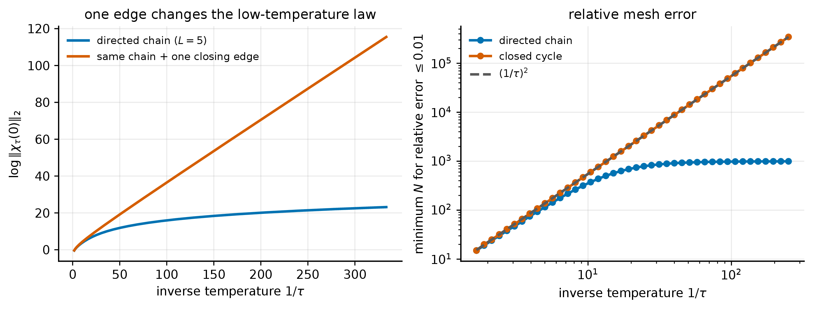
For 2, \(\beta=T=1\), \(Z\sim N(0,1)\), and \(\widehat\xi_n=Z/\sqrt n\). The same Gaussian draws are used across the three temperature schedules at each \(n\).

At the largest simulated size \(n=2^{26}\), the mean absolute time-zero magnetizations are \(0.0503\), \(0.5229\), and \(0.9738\) in the stable, critical, and selection schedules. At \(t=T/2\) they are \(0.0048\), \(0.0233\), and \(0.1465\), consistent with the fixed-time convergence in 8. At \(n=10^{14}\), the relative errors of the leading and two-term logarithmic approximations in 52 are \(16.2\%\) and \(1.32\%\).

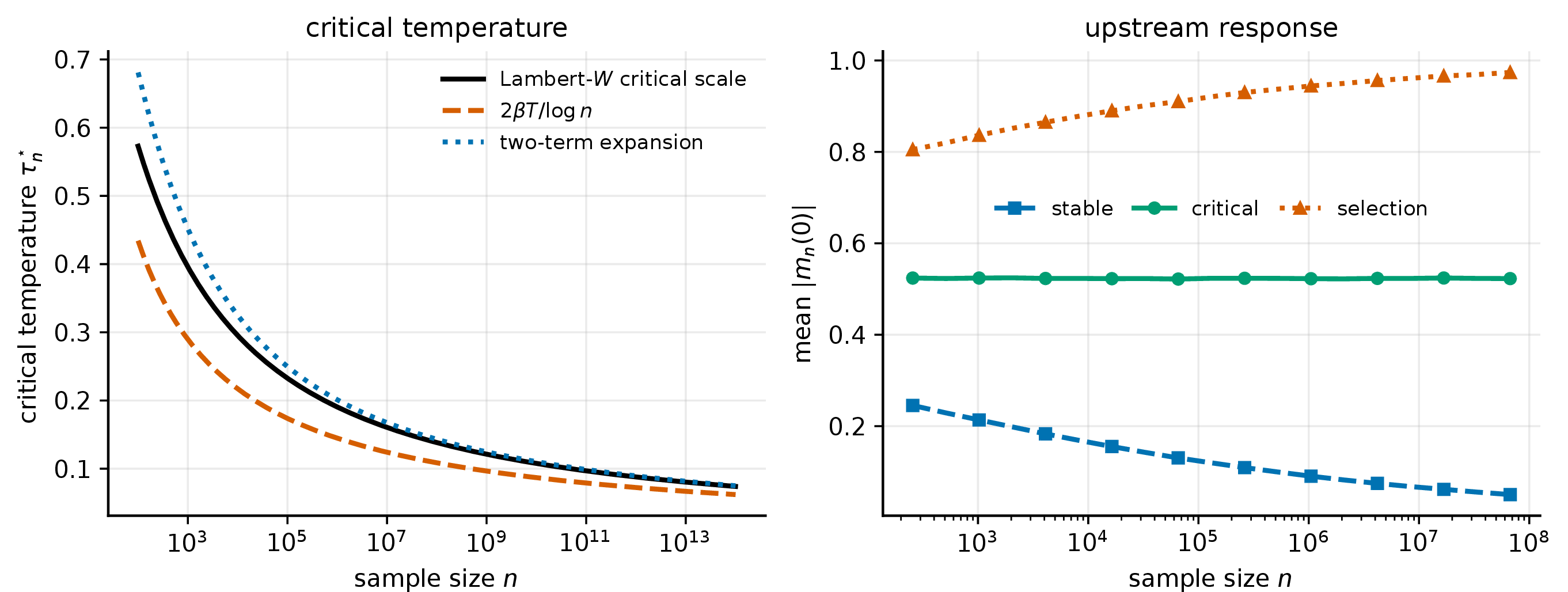
7 Discussion↩︎

On a DAG, a perturbation passes through only finitely many future selves. Under aligned forcing, a positive cycle permits repeated returns and can change polynomial susceptibility into exponential susceptibility. The bounded diffusion realizes both rates in arbitrary finite dimension. It also shows why a grid that is accurate at fixed temperature may fail under cooling: along a cyclic Perron mode, relative consistency requires \(N\tau^2\to\infty\).

Two limits of the present theory remain. The general parabolic argument gives \(e^{C/\tau^2}\), whereas the explicit graph model attains \(e^{C/\tau}\); whether state dependence can attain the larger rate is open. The statistical result assumes finite-dimensional model estimation and fixed positive temperature, except in the exactly solvable affine model. Action-dependent diffusion, nonsmooth estimators, and graph criteria for state-dependent equilibria remain unresolved.

Declaration of generative-AI assistance↩︎

OpenAI ChatGPT/Codex (July 2026) assisted with literature searches, drafting, editing, mathematical checks, and numerical code. The author assumes responsibility for all content.

Code availability↩︎

The accompanying reproducibility archive contains the seeded Python code and numerical output used to produce both figures and every reported numerical value.

Supplementary material. The supplement contains the detailed technical closures and classical bootstrap used in Sections 4–6.

References↩︎

---

1. Independent Researcher, Redwood City, CA (, https://orcid.org/0009-0008-1026-1083).↩︎