A Taxonomy of Distance Metrics for Time-Sensitive Importance Splitting
July 20, 2026
Abstract
ISPLIT evaluates the probabilities of rare events in non-Markovian models. It requires a heuristic IFUN that estimates the distance to the target. While including timer evaluations in the IFUN can substantially improve the effectiveness of ISPLIT, the existing time-sensitive IFUNs evaluate simulation states with respect to single sampled timer values. Thus, reaching highly important states requires simultaneously sampling specific combinations of timer values, yielding several unproductive simulation runs.
In this paper, we revisit time-sensitive ISPLIT with the goal of steering simulation runs towards important states. First, we study how timer values can be resampled conditioned on the elapsed time. The importance can be evaluated by considering the set of feasible timer values, decoupling importance estimation from timer samples. Second, we exploit the global age of a simulation to identify and prune the executions that can no longer reach the target within the remaining time budget. Together, these ideas lead to a taxonomy of distance metrics clarifying the role of timer bounds, resampling, and the global age. In particular, for models with unbounded timers, we show that time-sensitive IFUNs collapse to ordinary IFUNs under resampling. Experiments demonstrate that the proposed formulations substantially improve the accuracy of ISPLIT estimators.
1 Introduction↩︎
Reliability engineering provides methods and tools to assess risks in a variety of application domains [1], [2], performing quantitative evaluation of probabilistic models, e.g., the failure behavior of fault trees [3]. If any stochastic temporal parameter is non-exponentially distributed, the underlying stochastic process is non-Markovian [4], and the model is termed a non-Markovian model.
Analysis and simulation methods. Unlike the Markovian case, providing efficient solution techniques for the quantitative evaluation of non-Markovian models is considered significantly harder. Efficient quantitative evaluation methods do exist for restricted model classes such as non-Markovian models with an underlying semi-Markov process [5], at most one non-exponential timer in each state [6], [7], and an underlying Markov regenerative process with a bounded number of steps between subsequent regenerations [8]. These restrictions, however, limit the model expressiveness and do not fully address scalability challenges [9]–[11]. Thus, simulation, also known as SMC, remains the default approach for analyzing large non-Markovian models. In contrast to methods based on state-space enumeration, SMC produces an estimate \(\hat{\varphi}\) of some property \(\varphi\) s.t.\(\hat{\varphi}\in [l, u]\) with some confidence level \(\gamma\). While applicable to models with arbitrary size, it struggles to reliably estimate rare events [12]–[14].
ISPLIT is a prominent technique for reducing the variance of rare event estimations by layering (splitting) the state space so that reaching one layer from another one is not rare. The selection of layers is given by a heuristic IFUN, whose choice is the main deciding factor for the efficiency of ISPLIT. For a wide range of application scenarios, it has been demonstrated how an effective IFUN can be derived automatically [9], [15].
Time-sensitive ISPLIT. A notable challenge in non-Markovian models is that the progress towards the target depends both on the system’s discrete logical state and on the continuous remaining times of the active timers. In [11], we addressed this challenge by incorporating concrete timer values into automatically generated IFUNs, increasing the amount of information available to ISPLIT while tying importance to a particular sampled realization of timer values.

Example 1. 1 shows a repairable DFT from [11]. It is made of two BEs: UPS (uninterruptible power supply) and AC (alternating current grid). The system failure is governed by a PAND gate, i.e., it occurs only if the attached BEs fail from left to right. Given the failure and repair time bounds of the BEs, for the shortest path, the UPS BE needs to fail twice near the lower bound \(9.8\), while the AC BE has to fail at the upper bound \(20\). So, an IFUN should assign a state for which this condition applies a higher importance than for other states, which can only be expressed by considering concrete timer values.
Thus, two states may receive significantly different importance values given the timer values. Reaching highly important states might occur quite rarely, as most of the probability mass is concentrated in realizations with low-importance values. This raises the question: How can we observe more important simulation runs?
.7ex plus .2ex minus .1ex -.5em Contributions. In this paper, we tackle the above problem by
resampling of timers conditioned on their elapsed time
exploiting the global age
. These variations lead to a plethora of distance metrics, whose role regarding timer bounds, resampling, and the global age can be categorized in a taxonomy.
Resampling. The usual simulation semantics of non-Markovian models samples timer values when they are newly enabled. When a timer elapses, the values of the other persistent timers are reduced by the elapsed time. Notably, there is no need to fix the value of a timer upon enabling. Conditioned on each timer’s elapsed time, the future behavior is independent of the past samples and captures the reachable timing choices that remain available. We refer to sampling from this conditioned distribution as resampling. Similar concepts exist for approximating distributions from a finite number of samples [16], [17]. Resampling enables us to enlarge the number of different timer samples that reach a high importance. Specifically, for evaluating the time-sensitive IFUN, we consider the maximum importance that is reachable given the possible timer evaluations.
We have a closer look at the special case of models where each timer has an infinite domain \([0, \infty)\), which equates to just considering in which order the active timers elapse. There, we show that IFUNs based on backwards reachability search behave equally in the time-agnostic as well as time-sensitive setting when resorting to resampling. For a simulation run where no resampling is used, we develop a more efficient data structure to compute the time-sensitive IFUN.
Global age. For time-bounded reachability properties, we exploit the global age, i.e., the elapsed simulation time, to decide if the target condition can be reached within the remaining time budget. By integrating the global time as an artificial timer, the simulation can dynamically detect when the target condition is no longer reachable and immediately terminate unfeasible realizations.
.7ex plus .2ex minus .1ex -.5em Structure. We start by reviewing relevant background in 2. Then, we focus on the main contributions in the paper, i.e., resampling of timers (3) and inclusion of the global age (4). The plethora of derived distance metrics is categorized in a taxonomy in 5. We evaluate our variants for challenging DFTs and a queueing network in 6 and draw our conclusions in 7.
2 Background↩︎
2.1 Input/Output Stochastic Automata↩︎
We specify every model as a network of IOSAs. Intuitively, these are automata with stochastic timers that can communicate with input/output actions, where urgent actions operate instantaneously:
Definition 1 (IOSA). An IOSA with urgency [18] is a tuple \(( \begingroup \begingroup\lccode`~=`, \lowercase{\endgroup \edef~{\mathchar\the\mathcode`, \penalty 0 \noexpand} }\mathcode`,="8000 \mathcal{L},\mathcal{A},\mathcal{T},\xrightarrow{{}},T_0,l_0 \endgroup )\) consisting of a denumerable set of locations* \(\mathcal{L}\) with \(l_0\in\mathcal{L}\) being the initial location; a denumerable set of actions \(\mathcal{A}\) partitioned into two sets of input \(\mathcal{A}^{\mathsf i}\) and output \(\mathcal{A}^{\mathsf o}\) actions, where \(\mathcal{A}^{\mathsf u}\subseteq\mathcal{A}\) denotes the set of urgent actions; a finite set of timers \(\mathcal{T}\) s.t.each \(t\in\mathcal{T}\) has an associated continuous probability measure \(\mu_t\) supported on \(\mathbb{R}_{\ge0}\), where \(T_0\subseteq\mathcal{T}\) denotes the set of initial timers; and a transition function \({\xrightarrow{{}}}\subseteq\mathcal{L}\times2^\mathcal{T}\times\mathcal{A}\times2^\mathcal{T}\times\mathcal{L}\) whose elements \(\langle l, T, a, T', l' \rangle\) are written as \(l\xrightarrow{{\raisebox{-1pt}[0pt][0pt]{\scriptstyle{\scriptscriptstyle T,a,T'}}}}l'\).*
We explicitly distinguish between locations and (simulation) states:
Definition 2 (State). A state* is a pair \(\langle l, \tau\rangle \in \mathcal{S}\) with \(\mathcal{S}=\mathcal{L} \times ((\mathbb{R}_{\geq 0} \;\dot{\cup}\;\{ \bot \})^{\mathcal{T}})\), made of a location \(l\) and a timer value function \(\tau\) yielding an evaluation for each timer. We term a timer \(t\in \mathcal{T}\) active if \(\tau(t) \neq \bot\) and inactive otherwise.*
A transition \(l\xrightarrow{{\raisebox{-1pt}[0pt][0pt]{\scriptstyle{\scriptscriptstyle T,a,T'}}}}l'\) represents either an external event (if \(a\in \mathcal{A}^{\mathsf i}\) is an input action; then \(T = \varnothing\)) or an internal event (if \(a\in \mathcal{A}^{\mathsf o}\) is an output action; then \(|T| = 1\) for non-urgent actions and \(|T| = 0\) for urgent actions), which triggers action \(a\) and starts new timers \(T'\).2 In the end, the full parallel composition of the IOSA network must not have any unresolved input actions [18]. We require that exactly one subset of timers \(T_l \subseteq \mathcal{T}\) is active in each location \(l\) [18], [19]. Thus, given a location \(l\), for all associated states \(s = \langle l, \tau\rangle\) and timers \(t\in \mathcal{T}\), it holds that \(\tau(t) = \bot\) iff \(t\not\in T_l\), viz., when a timer is not active in the current state, it takes the special value \(\bot\) that denotes an inactive timer. We assume that for each timer \(t\in\mathcal{T}\) we can provide its bounds \([a,b] \subseteq \mathbb{Q}_{\geq 0}\cup \{\infty\}\):
Definition 3 (Timer bounds). When enumerating the \(n = |T_l|\) active timers of a location \(l\) as \(t_1, ..., t_n \in T_l\), we denote with \(a_i\in \mathbb{Q}_{\geq 0}\) the lower bound and with \(b_i\in \mathbb{Q}_{\geq 0}\cup \{\infty\}\) the upper bound of timer \(t_i\) for \(i \in \{1, ..., n\}\).
2.2 State Classes↩︎
To determine the minimum number of transitions needed to reach the target given the current timer values, the work of [11] used SCs [20]:
Definition 4 (SC). An SC \(\Sigma = \langle l, D \rangle\) consists of a location \(l \in \mathcal{L}\) and a joint domain \(D\) for the active timers in \(l\), i.e., the timers in \(T_l\).
The domain \(D\) of an SC \(\Sigma = \langle l, D \rangle\) collects the (infinite) possible timer values. It can be efficiently encoded as a DBM zone, i.e., the solution of a set of linear inequalities constraining the difference between two timers (with \(t_\star\) being a fictitious timer denoting the time when \(\Sigma\) is entered): \[\begin{align} D = \{ \tau(t_i) -\tau(t_j) \leq b_{ij} \quad \forall \, t_i, t_j \in T_{l} \cup\{t_{\star}\}witht_i \neq t_j\} \label{eq:DBM} \end{align}\tag{1}\]
To compute a distance metric that counts the number of transitions to reach the target, we perform backwards reachability search from the target locations. For each SC \(\Sigma' = \langle l', D'\rangle\) and incoming transition \(l\xrightarrow{{\raisebox{-1pt}[0pt][0pt]{\scriptstyle{\scriptscriptstyle T,a,T'}}}}l'\), we compute the predecessor SC \(\Sigma = \langle l, D\rangle\) and derive its distance metric \(\omega_T(\Sigma)\) as the minimum number of transitions needed to reach the target locations from \(\Sigma\). The predecessor calculations effectively resort to computing the weakest precondition, i.e., all states of \(\langle l, D\rangle\) end up in \(\langle l', D'\rangle\) after taking the transition. Details for the calculation can be found in [11] and in 8. During backwards reachability search, we can eliminate redundant information, e.g., if for one location \(l\) we have two SCs \(\Sigma_1=\langle l, D_1\rangle\) and \(\Sigma_2=\langle l, D_2\rangle\) such that \(D_1 \supseteq D_2\) and \(\omega_T(\Sigma_1) \leq \omega_T(\Sigma_2)\), so \(\Sigma_1\) strictly includes \(\Sigma_2\), we can omit \(\Sigma_2\). Analogously, by performing forwards search from the initial state with SCs, we can determine via SCs the set of states (locations and timer values) that are reachable during a simulation run [20].
We can evaluate the distance (i.e., the minimum number of steps to reach the target given the timer constraints) of a state \(s=\langle l,\tau \rangle\) as the minimum distance to the target among those of the SCs which \(s\) belongs to, i.e., \(d_T \colon \mathcal{S} \rightarrow \mathbb{N}_0 \cup \{\infty\}\) with \(d_T(s) = \min_{\Sigma \,\mid\, s \in \Sigma} \omega_T(\Sigma)\) (\(d_T\) is an acronym for distance timed) and \(d_T(s) = \infty\) if \(s\) is not contained in any SC \(\Sigma\). A state \(s=\langle l,\tau \rangle\) belongs to an SC \(\Sigma = \langle l',D \rangle\) (which we write as \(s \in \Sigma\)) if \(l=l'\) and the timer values defined by the timer value function \(\tau\) satisfy \(D\) (denoted with \(\tau \in D\)), which can be easily checked by evaluating all inequalities encoded in \(D\) (runtime \(\mathcal{O}(|T_l|^2)\)).
By laying a probability density over domain \(D\), we can quantify the probability of timer evaluations through SSCs [8], [21]:
Definition 5 (SSCs). An SSC is a tuple \(\Sigma = \langle l,D,f\rangle\) where \(l\), \(D\) are defined as for SCs and \(f : (\mathbb{R}_{\geq 0})^{|T_l|} \rightarrow \mathbb{R}_{\geq 0}\) is the PDF (immediately after the previous transition) of the random vector of the times-to-fire \(\tau\) of timers \(t_1, ..., t_n \in T_l\) enabled in \(l\).
Similarly to SCs, we can enumerate the set of reachable SSCs from the initial state by a forwards search from the initial state. This, for example, allows us to compute time-bounded reachability probabilities exactly, however, with significant costs due to the state-space explosion and complexity of representing SSCs.
2.3 Rare Event Simulation↩︎
Statistical model checking. In SMC, evaluating bounded reachability metrics boils down to the sampling of simulation traces, i.e., a sequence \(x_i = \{\langle l_j, \tau_j\rangle\}_{j=0}^{n_i}\) of states with locations \(l_j\) and timer values \(\tau_j\), so that \(x_i\) either visits a set of goal locations \(\mathcal{L}_{g}\) or not [22]. An unbiased estimator for the probability of reaching \(\mathcal{L}_{g}\) is then given by \(y_i = 1 \mathop{\mathsf{\underline{if}}} \exists j.\, l_j \in \mathcal{L}_g \mathop{\mathsf{\underline{else}}} 0\). For robustness, such point estimates are accompanied by an (asymptotic) statistical correctness guarantee, typically a CI \([l, u] \subseteq \mathbb{R}\) with confidence level \(\gamma\).
Importance splitting. For rare events, however, regular SMC needs an unfeasible number of samples to provide a tight CI. This problem can be alleviated by using RES methods, which can be categorized as IS and ISPLIT. IS modifies the underlying probability model such that the event of interest is more likely. While sophisticated automated methods exist for Markovian models, applying them to non-Markovian models is seen as significantly more challenging [23], [24]. Instead, we focus in this work on ISPLIT methods, which partition the state space into layers surrounding the goal states \(\mathcal{S}_g\subsetneq\mathcal{S}\). This is done using an IFUN \(f\colon\mathcal{S}\to\mathbb{N}_0 \cup \{-\infty\}\) that maps each state to an importance value (or indicates that the target is unreachable by the value \(-\infty\)). For ISPLIT, there exist multiple variations [15], [25], predominantly Fixed Effort and RESTART [26], [27]. In short, Fixed Effort iteratively starts from the selection of simulation runs that reached the next importance level, while RESTART merges split simulation runs when falling below a certain importance level.
Importance function derivation. A general automated approach to derive an IFUN uses backwards reachability search, i.e., a function \(d \colon \mathcal{S} \to \mathbb{N}_0 \cup \{\infty\}\) with \(d(\langle l, \tau\rangle) = \omega(l)\) that counts the number of needed transitions to the target, arriving at the IFUN \(f(s) \doteq \max_{s'\in \mathcal{S}, d(s')<\infty} \{d(s')\} - d(s)\) [15]. This concept straightforwardly translates to a time-sensitive setting using \(d_T \colon \mathcal{S} \rightarrow \mathbb{N}_0 \cup \{\infty\}\) (from 2.2) to arrive at the IFUN \(f_T(s) \doteq \max_{s' \in \mathcal{S}, d_T(s')<\infty} \{d_T(s')\} - d_T(s)\).
Threshold selection. The practical efficiency of ISPLIT strongly depends on the choice of importance levels (called thresholds) at which simulation runs are split. Too few thresholds lead to extinction (i.e., most runs fail to reach the target), whereas too many cause a significant performance overhead. Most methods for automatically computing thresholds [15], [28] start from the initial location and estimate level-up probabilities to determine the thresholds to include.
3 Resampling of Timers↩︎
This section is concerned with the first part of our main contribution, i.e., studying how the possibility of resampling timers influences the idea of time-sensitive ISPLIT. After explaining the general concept, we consider models with unbounded timers in 3.1 and the adaptations for threshold selection in 3.2.
As we can newly determine the value of each timer under the condition that a deterministic time has elapsed, we do not consider the currently sampled timer values, but the range of timer values that is possible given the elapsed time:
Definition 6 (Elapsed time). For a state \(s = \langle l, \tau\rangle \in \mathcal{S}\), \(\tau_{\textit{elp}} \in (\mathbb{R}_{\geq 0} \;\dot{\cup}\;\{ \bot \})^{\mathcal{T}}\) denotes the elapsed time* for each timer. Furthermore, we write \(s_{\textit{elp}} = \langle l, \tau_{\textit{elp}}\rangle\) for a location with elapsed time information.*
We determine \(\tau_\textit{elp}\) for each timer during a (forwards) simulation run as follows: In the initial state, no time has elapsed, so we set \(\tau_\textit{elp}(t) = 0\) for all \(t\in T_0\). Otherwise, consider a location \(l\) with elapsed time \(\tau_\textit{elp}\), concrete timer values \(\tau\), and outgoing transition \(l\xrightarrow{{\raisebox{-1pt}[0pt][0pt]{\scriptstyle{\scriptscriptstyle T,a,T'}}}}l'\) with \(T = \{t\}\). Then, the elapsed time of taking this transition is given by the value of the elapsed timer, i.e. \(\Delta = \tau(t)\). For the successor state with elapsed timer values \(s'_{\textit{elp}} = \langle l', \tau'_\textit{elp}\rangle\) it holds for all (newly enabled) timers \(t_i\in T' \colon \tau'_\textit{elp}(t_i) = 0\) and for all (persistent) timers \(t_i \in T_{l'} \backslash T' \colon \tau'_\textit{elp}(t_i) = \tau_\textit{elp}(t_i) + \Delta\).
Given the elapsed time, we can compute the lower bound of each timer as \(\tau_{\textit{min}} \in (\mathbb{R}_{\geq 0} \;\dot{\cup}\;\{ \bot \})^{\mathcal{T}}\) with \(\tau_{\textit{min}}(t_i) = \max(0, a_i - \tau_{\textit{elp}}(t_i))\) for \(t_i \in T_l\) and the upper bound \(\tau_{\textit{max}} \in (\mathbb{R}_{\geq 0} \;\dot{\cup}\;\{ \infty, \bot \})^{\mathcal{T}}\) with \(\tau_{\textit{max}}(t_i) = b_i - \tau_{\textit{elp}}(t_i)\).3
We define the timed distance metric under resampling as the regular minimum timed distance achievable by resampling the timers of the current state. This corresponds to the highest regular importance achievable by resampling. To formally define this metric, we observe that, depending on the value of \(\tau_\textit{elp}\), \(s_\textit{elp}\) induces an SC containing the potential timer values reachable by resampling:
Definition 7 (Induced state class). The induced SC of a state \(s = \langle l, \tau\rangle\) is the SC \(\Sigma_{s_\textit{elp}} = \langle l, D\rangle\) with domain \(D = \bigtimes_{t_i \in T_{l}} [\tau_{\textit{min}}(t_i), \tau_{\textit{max}}(t_i)]\).
As for the initial SC in the SC graph for forwards reachability analysis [8], [20], [21], the domain \(D\) has a hyper-rectangular shape as the individual timers are solely shifted by a time constant and thus remain independent. For the formal definition of the timed distance metric under resampling, we consider the minimum distance attainable by any state that is possible by resampling the current timers:
Definition 8 (Time-sensitive distance with resampling). Consider a state \(s = \langle l, \tau\rangle\) with elapsed time information \(s_{\textit{elp}} = \langle l, \tau_{\textit{elp}}\rangle\). Then, the timed distance metric under resampling is defined as \(d^{r}_{T}(s) = \min_{s'\in \Sigma_{s_\textit{elp}}} d_{T}(s')\).
Since \(d_{T}(s)\) is evaluated by iterating over the SCs associated with location \(l\), we can efficiently evaluate \(d^{r}_{T}(s)\) in a similar vein: We determine the SC with the smallest distance to the target that intersects with the induced SC \(\Sigma_{s_\textit{elp}} = \langle l, D\rangle\), formally \(d^{r}_{T}(s) = \min_{\Sigma = \langle l', D'\rangle \,\mid\, l=l'\wedge D\cap D' \neq \varnothing} \omega_T(\Sigma)\) (see 2.2). Note that checking if a point lies inside the domain spanned by a DBM zone has the same computational complexity as checking if the domains of two DBM zones with equal size intersect [20], [29], namely for \(n\) timers a runtime of \(\mathcal{O}(n^2)\).
Moreover, an orthogonal perspective can be achieved by considering the probability densities associated with each timer, as \(s_\textit{elp}\) also induces an SSC:
Definition 9 (Induced stochastic state class). Consider \(s_\textit{elp} = \langle l, \tau_\textit{elp}\rangle\). For a timer \(t_i \in T_l\), let \(f_i : [a_i, b_i] \rightarrow \mathbb{R}_{\geq 0}\) be its PDF for the corresponding probability measure \(\mu_{t_i}\). We use \(x_i\) for the variable describing the value of timer \(t_i\), i.e., \(\tau(t_i)\). Then, the induced SSC is the SSC \(\langle l, D, f\rangle\) with \(D\) defined as in 7 and \[f(x_1, ..., x_n) = \prod_{i=1}^{n} \underbrace{\frac{1}{\int_{\max(a_i, \tau_\textit{elp}(t_i))}^{b_i}f_i(x)dx}}_{\text{Normalization constant}} \cdot \underbrace{f_i(x_i + \tau_{\textit{elp}}(t_i))}_{\substack{\text{Marginal}\\ \text{distribution}}} \text{.}\]
As for the induced SC, the individual timers of the SSC are stochastically independent. Thus, each timer can be resampled individually, see 9.
![Figure 2: Selected SCs from backwards reachability search in the toy example from 1. Note the unequal axis scales in [fig:running-ex-scs2].](/article/2607.17939/_pdflatex/mcjgxkvb.png "fig:")
Example 2. We revisit the toy example from 1 in 2, where [fig:running-ex-scs-model] shows a part of the corresponding synchronized IOSA model. We denote with \(u\mathchoice {\text{\smaller[2]\color{Red}\ding{55}}} {\text{\smaller[2]\color{Red}\ding{55}}} {\scalebox{0.7}{\text{\smaller[2]\color{Red}\ding{55}}}} {\scalebox{0.5}{\text{\smaller[2]\color{Red}\ding{55}}}}\)/\(u\mathchoice {\text{\smaller[3]\color{OliveGreen}\faWrench}} {\text{\smaller[3]\color{OliveGreen}\faWrench}} {\scalebox{0.7}{\text{\smaller[3]\color{OliveGreen}\faWrench}}} {\scalebox{0.5}{\text{\smaller[3]\color{OliveGreen}\faWrench}}}\) and \(a\mathchoice {\text{\smaller[2]\color{Red}\ding{55}}} {\text{\smaller[2]\color{Red}\ding{55}}} {\scalebox{0.7}{\text{\smaller[2]\color{Red}\ding{55}}}} {\scalebox{0.5}{\text{\smaller[2]\color{Red}\ding{55}}}}\)/\(a\mathchoice {\text{\smaller[3]\color{OliveGreen}\faWrench}} {\text{\smaller[3]\color{OliveGreen}\faWrench}} {\scalebox{0.7}{\text{\smaller[3]\color{OliveGreen}\faWrench}}} {\scalebox{0.5}{\text{\smaller[3]\color{OliveGreen}\faWrench}}}\) the failure/repair of the UPS and AC BEs. [fig:running-ex-scs-path] shows the shortest possible sequence from an initial state to the target, which requires two failures with timer values \(t_{u\mathchoice {\text{\smaller[2]\color{Red}\ding{55}}} {\text{\smaller[2]\color{Red}\ding{55}}} {\scalebox{0.7}{\text{\smaller[2]\color{Red}\ding{55}}}} {\scalebox{0.5}{\text{\smaller[2]\color{Red}\ding{55}}}}}\) near the lower bound of \(9.8\) with intermediate repair \(t_{u\mathchoice {\text{\smaller[3]\color{OliveGreen}\faWrench}} {\text{\smaller[3]\color{OliveGreen}\faWrench}} {\scalebox{0.7}{\text{\smaller[3]\color{OliveGreen}\faWrench}}} {\scalebox{0.5}{\text{\smaller[3]\color{OliveGreen}\faWrench}}}}\) and the failure \(t_{a\mathchoice {\text{\smaller[2]\color{Red}\ding{55}}} {\text{\smaller[2]\color{Red}\ding{55}}} {\scalebox{0.7}{\text{\smaller[2]\color{Red}\ding{55}}}} {\scalebox{0.5}{\text{\smaller[2]\color{Red}\ding{55}}}}}\) near the upper bound of \(20\) (see 1). The DBM zones of \({\color{Orchid}D_1}\) to \({\color{Orange}D_5}\) are (computed via backwards search in [11]/8):
\({\color{Orchid}D_1} = \{ 0\leq \tau(t_{u\mathchoice {\text{\smaller[3]\color{OliveGreen}\faWrench}} {\text{\smaller[3]\color{OliveGreen}\faWrench}} {\scalebox{0.7}{\text{\smaller[3]\color{OliveGreen}\faWrench}}} {\scalebox{0.5}{\text{\smaller[3]\color{OliveGreen}\faWrench}}}})\leq 0.1 \}\)
\({\color{PineGreen}D_2} = \{ 0\leq \tau(t_{u\mathchoice {\text{\smaller[3]\color{OliveGreen}\faWrench}} {\text{\smaller[3]\color{OliveGreen}\faWrench}} {\scalebox{0.7}{\text{\smaller[3]\color{OliveGreen}\faWrench}}} {\scalebox{0.5}{\text{\smaller[3]\color{OliveGreen}\faWrench}}}})\leq 0.1\wedge 0\leq \tau(t_{a\mathchoice {\text{\smaller[2]\color{Red}\ding{55}}} {\text{\smaller[2]\color{Red}\ding{55}}} {\scalebox{0.7}{\text{\smaller[2]\color{Red}\ding{55}}}} {\scalebox{0.5}{\text{\smaller[2]\color{Red}\ding{55}}}}}) \leq 0.1\wedge 0\leq \tau(t_{u\mathchoice {\text{\smaller[3]\color{OliveGreen}\faWrench}} {\text{\smaller[3]\color{OliveGreen}\faWrench}} {\scalebox{0.7}{\text{\smaller[3]\color{OliveGreen}\faWrench}}} {\scalebox{0.5}{\text{\smaller[3]\color{OliveGreen}\faWrench}}}}) - \tau(t_{a\mathchoice {\text{\smaller[2]\color{Red}\ding{55}}} {\text{\smaller[2]\color{Red}\ding{55}}} {\scalebox{0.7}{\text{\smaller[2]\color{Red}\ding{55}}}} {\scalebox{0.5}{\text{\smaller[2]\color{Red}\ding{55}}}}})\leq 0.1\}\)
\({\color{Blue}D_3} = \{0\leq \tau(t_{u\mathchoice {\text{\smaller[2]\color{Red}\ding{55}}} {\text{\smaller[2]\color{Red}\ding{55}}} {\scalebox{0.7}{\text{\smaller[2]\color{Red}\ding{55}}}} {\scalebox{0.5}{\text{\smaller[2]\color{Red}\ding{55}}}}})\leq 12\wedge0 \leq \tau(t_{a\mathchoice {\text{\smaller[2]\color{Red}\ding{55}}} {\text{\smaller[2]\color{Red}\ding{55}}} {\scalebox{0.7}{\text{\smaller[2]\color{Red}\ding{55}}}} {\scalebox{0.5}{\text{\smaller[2]\color{Red}\ding{55}}}}})\leq 12.1\wedge -0.1\leq \tau(t_{u\mathchoice {\text{\smaller[2]\color{Red}\ding{55}}} {\text{\smaller[2]\color{Red}\ding{55}}} {\scalebox{0.7}{\text{\smaller[2]\color{Red}\ding{55}}}} {\scalebox{0.5}{\text{\smaller[2]\color{Red}\ding{55}}}}})-\tau(t_{a\mathchoice {\text{\smaller[2]\color{Red}\ding{55}}} {\text{\smaller[2]\color{Red}\ding{55}}} {\scalebox{0.7}{\text{\smaller[2]\color{Red}\ding{55}}}} {\scalebox{0.5}{\text{\smaller[2]\color{Red}\ding{55}}}}})\leq 0 \}\)
\({\color{Red}D_4} = \{ 0\leq \tau(t_{u\mathchoice {\text{\smaller[3]\color{OliveGreen}\faWrench}} {\text{\smaller[3]\color{OliveGreen}\faWrench}} {\scalebox{0.7}{\text{\smaller[3]\color{OliveGreen}\faWrench}}} {\scalebox{0.5}{\text{\smaller[3]\color{OliveGreen}\faWrench}}}}) \leq 0.1 \wedge 9.8\leq \tau(t_{a\mathchoice {\text{\smaller[2]\color{Red}\ding{55}}} {\text{\smaller[2]\color{Red}\ding{55}}} {\scalebox{0.7}{\text{\smaller[2]\color{Red}\ding{55}}}} {\scalebox{0.5}{\text{\smaller[2]\color{Red}\ding{55}}}}})\leq 12.2 \wedge -12.1\leq \tau(t_{u\mathchoice {\text{\smaller[3]\color{OliveGreen}\faWrench}} {\text{\smaller[3]\color{OliveGreen}\faWrench}} {\scalebox{0.7}{\text{\smaller[3]\color{OliveGreen}\faWrench}}} {\scalebox{0.5}{\text{\smaller[3]\color{OliveGreen}\faWrench}}}}) - \tau(t_{a\mathchoice {\text{\smaller[2]\color{Red}\ding{55}}} {\text{\smaller[2]\color{Red}\ding{55}}} {\scalebox{0.7}{\text{\smaller[2]\color{Red}\ding{55}}}} {\scalebox{0.5}{\text{\smaller[2]\color{Red}\ding{55}}}}})\leq -9.8\}\)
\({\color{Orange}D_5} = \{0\leq \tau(t_{u\mathchoice {\text{\smaller[2]\color{Red}\ding{55}}} {\text{\smaller[2]\color{Red}\ding{55}}} {\scalebox{0.7}{\text{\smaller[2]\color{Red}\ding{55}}}} {\scalebox{0.5}{\text{\smaller[2]\color{Red}\ding{55}}}}})\leq 10.2\wedge 9.8\leq \tau(t_{a\mathchoice {\text{\smaller[2]\color{Red}\ding{55}}} {\text{\smaller[2]\color{Red}\ding{55}}} {\scalebox{0.7}{\text{\smaller[2]\color{Red}\ding{55}}}} {\scalebox{0.5}{\text{\smaller[2]\color{Red}\ding{55}}}}})\leq 20 \wedge -12.2\leq \tau(t_{u\mathchoice {\text{\smaller[2]\color{Red}\ding{55}}} {\text{\smaller[2]\color{Red}\ding{55}}} {\scalebox{0.7}{\text{\smaller[2]\color{Red}\ding{55}}}} {\scalebox{0.5}{\text{\smaller[2]\color{Red}\ding{55}}}}})-\tau(t_{a\mathchoice {\text{\smaller[2]\color{Red}\ding{55}}} {\text{\smaller[2]\color{Red}\ding{55}}} {\scalebox{0.7}{\text{\smaller[2]\color{Red}\ding{55}}}} {\scalebox{0.5}{\text{\smaller[2]\color{Red}\ding{55}}}}})\leq -9.8 \}\)
At simulation start, the values for the initial timers \(t_{u\mathchoice {\text{\smaller[2]\color{Red}\ding{55}}} {\text{\smaller[2]\color{Red}\ding{55}}} {\scalebox{0.7}{\text{\smaller[2]\color{Red}\ding{55}}}} {\scalebox{0.5}{\text{\smaller[2]\color{Red}\ding{55}}}}}\) and \(t_{a\mathchoice {\text{\smaller[2]\color{Red}\ding{55}}} {\text{\smaller[2]\color{Red}\ding{55}}} {\scalebox{0.7}{\text{\smaller[2]\color{Red}\ding{55}}}} {\scalebox{0.5}{\text{\smaller[2]\color{Red}\ding{55}}}}}\) are (uniformly) sampled from \({\color{black!20!gray}D'_1} = \{9.8 \leq \tau(t_{u\mathchoice {\text{\smaller[2]\color{Red}\ding{55}}} {\text{\smaller[2]\color{Red}\ding{55}}} {\scalebox{0.7}{\text{\smaller[2]\color{Red}\ding{55}}}} {\scalebox{0.5}{\text{\smaller[2]\color{Red}\ding{55}}}}}) \leq 12 \wedge 18\leq \tau(t_{a\mathchoice {\text{\smaller[2]\color{Red}\ding{55}}} {\text{\smaller[2]\color{Red}\ding{55}}} {\scalebox{0.7}{\text{\smaller[2]\color{Red}\ding{55}}}} {\scalebox{0.5}{\text{\smaller[2]\color{Red}\ding{55}}}}}) \leq 20 \}\), i.e., the Cartesian product of the domains of \(\tau(t_{u\mathchoice {\text{\smaller[2]\color{Red}\ding{55}}} {\text{\smaller[2]\color{Red}\ding{55}}} {\scalebox{0.7}{\text{\smaller[2]\color{Red}\ding{55}}}} {\scalebox{0.5}{\text{\smaller[2]\color{Red}\ding{55}}}}})\) and \(\tau(t_{a\mathchoice {\text{\smaller[2]\color{Red}\ding{55}}} {\text{\smaller[2]\color{Red}\ding{55}}} {\scalebox{0.7}{\text{\smaller[2]\color{Red}\ding{55}}}} {\scalebox{0.5}{\text{\smaller[2]\color{Red}\ding{55}}}}})\). Assume the following sampled values:
- \({\color{Brown}\tau_1} = \{t_{u\mathchoice {\text{\smaller[2]\color{Red}\ding{55}}} {\text{\smaller[2]\color{Red}\ding{55}}} {\scalebox{0.7}{\text{\smaller[2]\color{Red}\ding{55}}}} {\scalebox{0.5}{\text{\smaller[2]\color{Red}\ding{55}}}}} \mapsto 9.9, t_{a\mathchoice {\text{\smaller[2]\color{Red}\ding{55}}} {\text{\smaller[2]\color{Red}\ding{55}}} {\scalebox{0.7}{\text{\smaller[2]\color{Red}\ding{55}}}} {\scalebox{0.5}{\text{\smaller[2]\color{Red}\ding{55}}}}} \mapsto 19.9\}\) (shorthand notation for a function \({\color{Brown}\tau_1}\) that satisfies \({\color{Brown}\tau_1}(t_{u\mathchoice {\text{\smaller[2]\color{Red}\ding{55}}} {\text{\smaller[2]\color{Red}\ding{55}}} {\scalebox{0.7}{\text{\smaller[2]\color{Red}\ding{55}}}} {\scalebox{0.5}{\text{\smaller[2]\color{Red}\ding{55}}}}}) = 9.9\), \({\color{Brown}\tau_1}(t_{a\mathchoice {\text{\smaller[2]\color{Red}\ding{55}}} {\text{\smaller[2]\color{Red}\ding{55}}} {\scalebox{0.7}{\text{\smaller[2]\color{Red}\ding{55}}}} {\scalebox{0.5}{\text{\smaller[2]\color{Red}\ding{55}}}}}) = 19.9\), and \({\color{Brown}\tau_1}(t) = \bot\) for any other \(t\in \mathcal{T}\))
Then, the distance evaluation for time-sensitive ISPLIT operates as follows:
**Regular simulation:* It holds that \({\color{Brown}\tau_1} \in {\color{Orange}D_5}\), so \(d_T(\langle l_{ua}, {\color{Brown}\tau_1}\rangle) = 4\). On the other hand, both \({\color{Brown}\tau_2} \not\in {\color{Orange}D_5}\) and \({\color{Brown}\tau_3} \not\in {\color{Orange}D_5}\), so it holds \(d_T(\langle l_{ua}, {\color{Brown}\tau_2}\rangle) > 4\) and \(d_T(\langle l_{ua}, {\color{Brown}\tau_3}\rangle) > 4\). Eventually, we obtain \(d_T(\langle l_{ua}, {\color{Brown}\tau_2}\rangle) = d_T(\langle l_{ua}, {\color{Brown}\tau_3}\rangle) = 14\).*
**With resampling:* In the initial state, the already elapsed time is \(\tau_\textit{elp} = \{t_{u\mathchoice {\text{\smaller[2]\color{Red}\ding{55}}} {\text{\smaller[2]\color{Red}\ding{55}}} {\scalebox{0.7}{\text{\smaller[2]\color{Red}\ding{55}}}} {\scalebox{0.5}{\text{\smaller[2]\color{Red}\ding{55}}}}} \mapsto 0, t_{a\mathchoice {\text{\smaller[2]\color{Red}\ding{55}}} {\text{\smaller[2]\color{Red}\ding{55}}} {\scalebox{0.7}{\text{\smaller[2]\color{Red}\ding{55}}}} {\scalebox{0.5}{\text{\smaller[2]\color{Red}\ding{55}}}}} \mapsto 0\}\) and the SC domain is \({\color{black!20!gray}D'_1}\), which intersects with \({\color{Orange}D_5}\). So, we obtain for all timer evaluations \(d^r_T(\langle l_{ua}, {\color{Brown}\tau_1}\rangle) = d^r_T(\langle l_{ua}, {\color{Brown}\tau_2}\rangle) = d^r_T(\langle l_{ua}, {\color{Brown}\tau_3}\rangle) = 4\).*
Depending on whether we choose \({\color{Brown}\tau_1}\)/\({\color{Brown}\tau_2}\) (\(t_{u\mathchoice {\text{\smaller[2]\color{Red}\ding{55}}} {\text{\smaller[2]\color{Red}\ding{55}}} {\scalebox{0.7}{\text{\smaller[2]\color{Red}\ding{55}}}} {\scalebox{0.5}{\text{\smaller[2]\color{Red}\ding{55}}}}} \mapsto 9.9\)) or \({\color{Brown}\tau_3}\) (\(t_{u\mathchoice {\text{\smaller[2]\color{Red}\ding{55}}} {\text{\smaller[2]\color{Red}\ding{55}}} {\scalebox{0.7}{\text{\smaller[2]\color{Red}\ding{55}}}} {\scalebox{0.5}{\text{\smaller[2]\color{Red}\ding{55}}}}} \mapsto 11.5\)), however, the elapsed time \(\Delta\) and the induced SC in the location \(l_{\ifmmode\text{\sout{u}}\else\sout{u}\fi a}\) differ:
For \({\color{Brown}\tau_1}\)/\({\color{Brown}\tau_2}\), \(\Delta = 9.9\), the elapsed time information for the subsequent state is \(\tau'_{\textit{elp}} = \{t_{u\mathchoice {\text{\smaller[3]\color{OliveGreen}\faWrench}} {\text{\smaller[3]\color{OliveGreen}\faWrench}} {\scalebox{0.7}{\text{\smaller[3]\color{OliveGreen}\faWrench}}} {\scalebox{0.5}{\text{\smaller[3]\color{OliveGreen}\faWrench}}}} \mapsto 0.0, t_{a\mathchoice {\text{\smaller[2]\color{Red}\ding{55}}} {\text{\smaller[2]\color{Red}\ding{55}}} {\scalebox{0.7}{\text{\smaller[2]\color{Red}\ding{55}}}} {\scalebox{0.5}{\text{\smaller[2]\color{Red}\ding{55}}}}} \mapsto 9.9\}\) and the domain of the induced SC \({\color{black!20!gray}D'_2} = \{0 \leq \tau(t_{u\mathchoice {\text{\smaller[3]\color{OliveGreen}\faWrench}} {\text{\smaller[3]\color{OliveGreen}\faWrench}} {\scalebox{0.7}{\text{\smaller[3]\color{OliveGreen}\faWrench}}} {\scalebox{0.5}{\text{\smaller[3]\color{OliveGreen}\faWrench}}}}) \leq 0.1 \wedge 8.1\leq \tau(t_{a\mathchoice {\text{\smaller[2]\color{Red}\ding{55}}} {\text{\smaller[2]\color{Red}\ding{55}}} {\scalebox{0.7}{\text{\smaller[2]\color{Red}\ding{55}}}} {\scalebox{0.5}{\text{\smaller[2]\color{Red}\ding{55}}}}}) \leq 10.1 \}\). The intersection \({\color{black!20!gray}D_2'} \cap {\color{red}D_4} \neq \varnothing\) is non-empty, leading to \(d^r_T(s') = 3\) for every \(s'\in \langle l_{\ifmmode\text{\sout{u}}\else\sout{u}\fi a}, {\color{black!20!gray}D_2'}\rangle\).
On the other hand, for \({\color{Brown}\tau_3}\), \(\Delta = 11.5\), \(\tau'_{\textit{elp}} = \{t_{u\mathchoice {\text{\smaller[3]\color{OliveGreen}\faWrench}} {\text{\smaller[3]\color{OliveGreen}\faWrench}} {\scalebox{0.7}{\text{\smaller[3]\color{OliveGreen}\faWrench}}} {\scalebox{0.5}{\text{\smaller[3]\color{OliveGreen}\faWrench}}}} \mapsto 0.0, t_{a\mathchoice {\text{\smaller[2]\color{Red}\ding{55}}} {\text{\smaller[2]\color{Red}\ding{55}}} {\scalebox{0.7}{\text{\smaller[2]\color{Red}\ding{55}}}} {\scalebox{0.5}{\text{\smaller[2]\color{Red}\ding{55}}}}} \mapsto 11.5\}\), and the domain of the induced SC is \({\color{black!20!gray}D'_3} = \{0 \leq \tau(t_{u\mathchoice {\text{\smaller[3]\color{OliveGreen}\faWrench}} {\text{\smaller[3]\color{OliveGreen}\faWrench}} {\scalebox{0.7}{\text{\smaller[3]\color{OliveGreen}\faWrench}}} {\scalebox{0.5}{\text{\smaller[3]\color{OliveGreen}\faWrench}}}}) \leq 0.1 \wedge 6.5\leq \tau(t_{a\mathchoice {\text{\smaller[2]\color{Red}\ding{55}}} {\text{\smaller[2]\color{Red}\ding{55}}} {\scalebox{0.7}{\text{\smaller[2]\color{Red}\ding{55}}}} {\scalebox{0.5}{\text{\smaller[2]\color{Red}\ding{55}}}}}) \leq 8.5 \}\). As the intersection \({\color{black!20!gray}D_3'} \cap {\color{red}D_4} = \varnothing\) is empty, \(d^r_T(s') > 3\) for every \(s'\in \langle l_{\ifmmode\text{\sout{u}}\else\sout{u}\fi a}, {\color{black!20!gray}D_3'}\rangle\). With further exploration, we obtain \(d^r_T(s') = 13\).
Summarizing, resampling considers the set of possible timer values in a state, eradicating the need to sample all timer values correctly for a certain importance (see \({\color{Brown}\tau_1}\)). Practically, this leads to a lower variance per ISPLIT run (see 6).
3.1 Models with Unbounded Timers↩︎
This subsection is concerned with the timed distance metrics in the special case that each timer in the model has an infinite domain \([0, \infty)\). In fact, this property applies to a plethora of commonly used distributions, e.g., the Exponential, Erlang, or Weibull distribution. Although we can reuse the backwards reachability metric search for the timed distance \(d_T\) based on exploring the SC graph, dealing with DBM zones can induce a significant performance hit: For example (see 2.2), we perform strict inclusion checking during backwards reachability search with SCs to limit the explored state space. However, this approach could be further optimized: We could merge adjacent DBM zones (e.g., when \(D_1\cup D_2\) can be represented as a DBM zone again), or omit an SC \(\Sigma_1 = \langle l, D_1\rangle\) such that there exist SCs \(\Sigma_2 = \langle l, D_2\rangle\), …, \(\Sigma_k = \langle l, D_k\rangle\) (with \(k > 2\)) with lower distances to the target than \(\Sigma_1\) and \(D_1 \subseteq D_2 \cup \dots \cup D_k\). Although such operations would be strongly beneficial to reduce the SC graph size, their implementation is known to be considerably hard for DBM zones [29], rendering their use impractical.
Efficient data structure. For order-based distance metrics, denoted in the following as \(d_{O} \colon \mathcal{S}\rightarrow \mathbb{N}_0 \cup \{\infty\}\) (acronym for distance ordered), we develop a specialized data structure by observing that, in this case, any DBM zone can be captured by the union of elementary SCs that store an ordering of timers:
Definition 10 (Elementary state class for ordered distances). For a location \(l\) and an ordering of timers \(T_l\) encoded as permutation \(\sigma : T_l \rightarrow T_l\), the elementary SC* is \(\Sigma_{\sigma} = \langle l, D_{\sigma}\rangle\) with \(n=|T_l|\) timers and the elementary domain \[\begin{align} D_{\sigma} = \bigcap_{1\leq i\leq n - 1} \{ \tau(\sigma(t_i)) \leq \tau(\sigma(t_{i+1})) \} = \{ \tau(\sigma(t_1)) \leq \tau(\sigma(t_2)) \leq ... \leq \tau(\sigma(t_n)) \}\text{.} \end{align}\]*
Trivially, there exist \(|T_l|!\) elementary SCs for a location \(l\) as there are as many permutations for a list of \(|T_l|\) elements. By making use of the Lehmer code [30], we can index each permutation, leading to the bijection \(\lambda : \textit{Perm}(T_l) \rightarrow \{1, 2, ..., |T_l|!\}\). To calculate the metric \(d_{O}\), instead of working with DBM zones directly, we store for each location \(l\) an array of size \(|T_l|!\) that contains the value of the distance metric \(\omega_O(\Sigma)\) for every elementary SC \(\Sigma\). We start with the elementary SCs of the target locations and perform backwards reachability search as in [11]/8. Consequently, the size of the created SC graph lies in \(\mathcal{O}(\sum_{l\in \mathcal{L}} |T_l|!)\).
During simulation, the distance \(d_{O}\) can be evaluated for a state \(s = \langle l, \tau\rangle\) by determining the timer ordering permutation \(\sigma\), evaluating the Lehmer code \(\lambda(\sigma)\) (implemented in time \(\mathcal{O}(|T_l|^2)\)), and looking up the distance of \(\omega_O(\Sigma_\sigma)\).
Resampling for ordered distance metrics. Next, we focus on the following question: What changes when we apply resampling to ordered distance metrics? As every timer is unbounded, resampling can always arbitrarily change the order of timers. This raises the question: When working with unbounded timers, does resorting to time-sensitive IFUNs even make a difference? The answer is no, which is formalized as follows (where \(d^r_O(s) = \min_{s'\in \Sigma_{s_\textit{elp}}} d_{O}(s')\) as in 8):
Theorem 1. For every state \(s\in\mathcal{S}\) it holds that \(d(s) = d^r_O(s)\).
This result has practical implications: When working with unbounded timer domains, it suffices for resampling to construct the cheaper-to-compute regular distance metric. On the other hand, an ISPLIT run without resampling is on average faster, albeit with higher variance. The practical performance tradeoff between both approaches is discussed in 6.
3.2 Threshold Selection↩︎
Most threshold selection approaches for ISPLIT (see 2.3) start in the initial location and estimate the level-up probabilities. This requires that the initial states have (almost) the lowest possible importance value. However, in a time-sensitive setting, the initial states might have different importance values [15], [28].
Regular simulation. To find the states in the initial location with lowest importance, we sample \(n\) different initial states and record the importance values, from which we select the \(k\) lowest ones and note their importance range. In our experiments, we set \(n = 1000\) and \(k = 10\), which ensures that a wide range of possible importance values is covered, while preventing too expensive rejection sampling from the states with the lowest importance values. Only states with an importance value in the range of the \(k\) selected states are used as initial states.
With resampling. On the other hand, when using resampling, the importance value is the same for any initial state, as the elapsed time information \(\tau_{\textit{elp}}\) is equal, and thus the induced SC \(\Sigma_{\tau_{\textit{elp}}}\). Thus, no adjustments are necessary here.
4 Considering the Global Age↩︎
As the second part of our main contribution, we analyze how to incorporate global time into the time-sensitive framework. For time-bounded reachability analysis, the global time can be used to determine whether the target remains reachable within the available time budget. Otherwise, the corresponding simulation offspring can be pruned, significantly reducing simulation effort.
The basis for including the global time information is by means of an artificial timer that records the remaining time budget until the simulation time bound.
Definition 11 (Global age timer). We denote with \(t_\textit{age}\) the global age timer* recording the remaining time budget upon entering a state, and with \(\mathcal{T}_\textit{age} = \mathcal{T}\cup \{t_\textit{age}\}\) the set of all timers including the global age timer.*
This idea is a standard concept in forwards analysis with SCs or SSCs [8], [10]. In our backwards reachability search setting, timer elapsing is followed in the opposite direction. Thus, at the end of simulation, it reaches the lowest value \(0\), resulting in potential values of \(\tau(t_\textit{age})\) in \([0, \infty)\). Consequently, we extend the state space \(\mathcal{S}\) by a dimension for \(t_\textit{age}\), so \(\mathcal{S}_\textit{age} = \mathcal{L} \times ((\mathbb{R}_{\geq 0} \;\dot{\cup}\;\{ \bot \})^{\mathcal{T}} \times \mathbb{R}_{\geq 0})\).
Distance metrics. For a global time bound \(t_{\textit{age}}^{\textit{max}} \in \mathbb{R}_{\geq 0}\), we extend the distance metrics \(d_{T}\) (2.2) and \(d^r_{T}\) (3, 8), as well as \(d_{O}\) and \(d^r_{O}\) (3.1) with the following global age variants returning the minimum number of transitions needed to reach the target within the time budget \(t_\textit{age}^\textit{max}\):
\(d_{TG}\) and \(d^r_{TG}\) (for distance timed global), considering timer bounds
\(d_{OG}\) and \(d^r_{OG}\) (for distance order global), neglecting timer bounds
Analogously, the concept can be readily extended to transient probabilities, i.e., the probability of being at a target state exactly at a given time \(t_\textit{age}^\textit{max}\):
\(d_{TEG}\) and \(d^r_{TEG}\) (for distance timed exactly global), considering timer bounds
\(d_{OEG}\) and \(d^r_{OEG}\) (for distance order exactly global), neglecting timer bounds
State class adaptations. For the computation of the distance metrics \(\omega_{TG}(\Sigma)\), \(\omega_{OG}(\Sigma)\), \(\omega_{TEG}(\Sigma)\), and \(\omega_{OEG}(\Sigma)\) (naming scheme as above), we distinguish for all SCs \(\Sigma' = \langle l', D'\rangle\) between time-bounded and transient reachability queries:
For time-bounded queries (\(\omega_{TG}(\Sigma)\), \(\omega_{OG}(\Sigma)\)), no adjustments to the target SC \(\Sigma'\) as calculated in 8 and [11] need to be made, as the location \(l'\) can be left before the global time bound in a simulation run.
For transient reachability queries (\(\omega_{TEG}(\Sigma)\), \(\omega_{OEG}(\Sigma)\)), we must ensure that a simulation run does not leave \(l'\) before the end of the time bound. Thus, we restrict the domain \(D'\) of \(\Sigma'\) with \(D'_{E} = D' \cap (\bigcap_{t\in T_{l'}} \{ \tau(t) \geq \tau(t_{\textit{age}}) \})\).
For calculating the predecessor SC when inversely following a transition \(l\xrightarrow{{\raisebox{-1pt}[0pt][0pt]{\scriptstyle{\scriptscriptstyle T,a,T'}}}}l'\), no adjustments to the procedures in 8 and [11] need to be made. The restrictions imposed on \(t_\textit{age}\) and the other timers are updated implicitly.
For evaluating the importance of a state under consideration of resampling, one needs to consider: As \(t_\textit{age}\) is not a classical timer to which a probability distribution is assigned, it can also not be resampled and has a fixed value of \(\tau(t_\textit{age})\). Thus, we obtain as induced SC (adapted from 7):
Definition 12 (Induced state class with global age). The induced SC of \(s = \langle l, \tau\rangle\) (with global age) is the SC \(\Sigma_{s_\textit{elp}} = \langle l, D\rangle\) with domain \(D = (\bigtimes_{t_i \in T_{l}} [\tau_{\textit{min}}(t_i), \tau_{\textit{max}}(t_i)]) \times \{\tau(t_\textit{age})\}\).
The extension of the induced SSCs (cmp. 9) is analogous. For distance evaluation, we determine the SC with the smallest distance to the target from the SC graph (with global age) that intersects with the induced SC, as in 3.
Pruning. During backwards reachability search, we can prune SCs that are not reachable in the given time budget. Formally, when it holds for an SC \(\Sigma = \langle l, D\rangle\) that \(\min_{\tau \in D} \tau(t_\textit{age}) > t_\textit{age}^\textit{max}\), no further exploration is needed for this branch: The time budget does not suffice for a simulation run to intersect with \(\Sigma\).
Second, when during simulation the distance of a state \(s\) evaluates to \(\infty\), i.e., no SC has been found, a simulation offspring can be pruned. Note that an unbiased result requires the SC graph to be fully constructed. While this is also theoretically conceivable for distance metrics without incorporation of global timers, it is usually only effective with them, as (i) many models allow reaching the target from any location (pruning is solely possible when incorporating the time bound) and (ii) for tight time bounds, constructing the pruned SC graph might be cheaper than constructing the complete SC graph without age timer:
Example 3. We revisit the toy example in 1/2. Constructing the complete backwards SC graph without global age results in \(14\) locations and \(97\) SCs. For time-bounded reachability queries, the SC graph with global age and a time limit of \(t_{\textit{age}}^{\textit{max}} = 21\) only has \(43\) SCs when pruning SCs outside the time budget. For the initial location \(l_{ua}\), the domains \({\color{Blue}D_3}\) and \({\color{Orange}D_5}\) are updated:
\({\color{Blue}D_3} = \{0\leq \tau(t_{u\mathchoice {\text{\smaller[2]\color{Red}\ding{55}}} {\text{\smaller[2]\color{Red}\ding{55}}} {\scalebox{0.7}{\text{\smaller[2]\color{Red}\ding{55}}}} {\scalebox{0.5}{\text{\smaller[2]\color{Red}\ding{55}}}}})\leq 12\wedge0 \leq \tau(t_{a\mathchoice {\text{\smaller[2]\color{Red}\ding{55}}} {\text{\smaller[2]\color{Red}\ding{55}}} {\scalebox{0.7}{\text{\smaller[2]\color{Red}\ding{55}}}} {\scalebox{0.5}{\text{\smaller[2]\color{Red}\ding{55}}}}})\leq 12.1\wedge 0 \leq \tau(t_\textit{age}) \wedge -0.1\leq \tau(t_{u\mathchoice {\text{\smaller[2]\color{Red}\ding{55}}} {\text{\smaller[2]\color{Red}\ding{55}}} {\scalebox{0.7}{\text{\smaller[2]\color{Red}\ding{55}}}} {\scalebox{0.5}{\text{\smaller[2]\color{Red}\ding{55}}}}})-\tau(t_{a\mathchoice {\text{\smaller[2]\color{Red}\ding{55}}} {\text{\smaller[2]\color{Red}\ding{55}}} {\scalebox{0.7}{\text{\smaller[2]\color{Red}\ding{55}}}} {\scalebox{0.5}{\text{\smaller[2]\color{Red}\ding{55}}}}})\leq 0\wedge 0 \leq \tau(t_\textit{age}) - \tau(t_{u\mathchoice {\text{\smaller[2]\color{Red}\ding{55}}} {\text{\smaller[2]\color{Red}\ding{55}}} {\scalebox{0.7}{\text{\smaller[2]\color{Red}\ding{55}}}} {\scalebox{0.5}{\text{\smaller[2]\color{Red}\ding{55}}}}})\wedge 0 \leq \tau(t_\textit{age}) - \tau(t_{a\mathchoice {\text{\smaller[2]\color{Red}\ding{55}}} {\text{\smaller[2]\color{Red}\ding{55}}} {\scalebox{0.7}{\text{\smaller[2]\color{Red}\ding{55}}}} {\scalebox{0.5}{\text{\smaller[2]\color{Red}\ding{55}}}}}) \}\)
\({\color{Orange}D_5} = \{0\leq \tau(t_{u\mathchoice {\text{\smaller[2]\color{Red}\ding{55}}} {\text{\smaller[2]\color{Red}\ding{55}}} {\scalebox{0.7}{\text{\smaller[2]\color{Red}\ding{55}}}} {\scalebox{0.5}{\text{\smaller[2]\color{Red}\ding{55}}}}})\leq 10.2\wedge 9.8\leq \tau(t_{a\mathchoice {\text{\smaller[2]\color{Red}\ding{55}}} {\text{\smaller[2]\color{Red}\ding{55}}} {\scalebox{0.7}{\text{\smaller[2]\color{Red}\ding{55}}}} {\scalebox{0.5}{\text{\smaller[2]\color{Red}\ding{55}}}}})\leq 20 \wedge 9.8 \leq \tau(t_{\textit{age}}) \wedge -12.2\leq \tau(t_{u\mathchoice {\text{\smaller[2]\color{Red}\ding{55}}} {\text{\smaller[2]\color{Red}\ding{55}}} {\scalebox{0.7}{\text{\smaller[2]\color{Red}\ding{55}}}} {\scalebox{0.5}{\text{\smaller[2]\color{Red}\ding{55}}}}})-\tau(t_{a\mathchoice {\text{\smaller[2]\color{Red}\ding{55}}} {\text{\smaller[2]\color{Red}\ding{55}}} {\scalebox{0.7}{\text{\smaller[2]\color{Red}\ding{55}}}} {\scalebox{0.5}{\text{\smaller[2]\color{Red}\ding{55}}}}})\leq -9.8 \wedge 9.8 \leq \tau(t_{\textit{age}}) - \tau(t_{u\mathchoice {\text{\smaller[2]\color{Red}\ding{55}}} {\text{\smaller[2]\color{Red}\ding{55}}} {\scalebox{0.7}{\text{\smaller[2]\color{Red}\ding{55}}}} {\scalebox{0.5}{\text{\smaller[2]\color{Red}\ding{55}}}}}) \wedge 0 \leq \tau(t_{\textit{age}}) - \tau(t_{a\mathchoice {\text{\smaller[2]\color{Red}\ding{55}}} {\text{\smaller[2]\color{Red}\ding{55}}} {\scalebox{0.7}{\text{\smaller[2]\color{Red}\ding{55}}}} {\scalebox{0.5}{\text{\smaller[2]\color{Red}\ding{55}}}}}) \}\)
As in the initial state (cmp. domain \(D'_1\)) \(\tau(t_{u\mathchoice {\text{\smaller[2]\color{Red}\ding{55}}} {\text{\smaller[2]\color{Red}\ding{55}}} {\scalebox{0.7}{\text{\smaller[2]\color{Red}\ding{55}}}} {\scalebox{0.5}{\text{\smaller[2]\color{Red}\ding{55}}}}}) \geq 9.8\) and \(\tau(t_{a\mathchoice {\text{\smaller[2]\color{Red}\ding{55}}} {\text{\smaller[2]\color{Red}\ding{55}}} {\scalebox{0.7}{\text{\smaller[2]\color{Red}\ding{55}}}} {\scalebox{0.5}{\text{\smaller[2]\color{Red}\ding{55}}}}}) \geq 18\), a timer evaluation \(\tau\in {\color{Orange}D_5}\) must in particular fulfill \(\tau(t_\textit{age}) \geq \max(9.8+9.8, 18) = 19.6\). So, the time budget must be at least \(19.6\) such that we initially have \(d_{TG}(s) = 4\).
5 Taxonomy of Distance Metrics↩︎

To categorize the distance metrics from [sec:background,sec:resampling-timers,sec:global-age] into a taxonomy, we address the following question: How does adding information (e.g., timer bounds, global age) affect the resulting IFUN? Since these metrics estimate the distance to the target, adding information refines the estimate by excluding unfeasible paths, thus increasing the calculated distance. According to this, a lower distance estimate indicates a coarser approximation that falsely suggests a higher importance by ignoring additional information. This is formalized as follows:
Definition 13 (Distance metric granularity). We say that a distance metric \(d_A\) is at least as fine-grained as distance metric \(d_B\), denoted \(d_A \succeq d_B\), if it holds for all states \(s\in \mathcal{S}\) that \(d_A(s)\geq d_B(s)\).
The relation \(\preceq\) defines a partial order on the distance metrics. In particular, two distance metrics \(d_A\) and \(d_B\) can also be equivalent, denoted \(d_A \equiv d_B\), when it holds for all states \(s\in \mathcal{S}: d_A(s) = d_B(s)\). It has already been proven that \(d \equiv d^r_{O}\) in 1. Likewise, we can make the following further statements:
Theorem 2. The following granularity statements about distance metrics hold:
\(d \equiv d^r_{O} \equiv d^r_{OG} \equiv d^r_{OEG}\) (equivalence for order w/resampling);
\(d_O \preceq d_{OG} \preceq d_{OEG}\), \(d_T \preceq d_{TG} \preceq d_{TEG}\), \(d^r_T \preceq d^r_{TG} \preceq d^r_{TEG}\) (age inclusion);
\(d \preceq d_O\), \(d_O \preceq d_T\), \(d_{OG} \preceq d_{TG}\), \(d_{OEG} \preceq d_{TEG}\), \(d \preceq d^r_T\) (time granularity);
\(d^r_T \preceq d_T\), \(d^r_{TG} \preceq d_{TG}\), \(d^r_{TEG} \preceq d_{TEG}\) (resampling yes/no).
While we can compare a distance metric \(d_*\) with its resampling variant \(d_*^r\), note that, although \(d_* \succeq d_*^r\), \(d_*^r\) performs better as it incorporates resampling. For performance assessment, one should thus compare solely inside the \(d_*\) or \(d_*^r\) class.
3 categorizes all distance metrics presented in this paper, sorted by whether
the timer bounds are considered
resampling is used or not
the global age is considered
. There is no resampling variant of the metric \(d\) as \(d\) is time-agnostic by default. In the diagram, denotes \(d_A \preceq d_B\).

Example 4. Reconsider the toy example from 1/2. 4 shows how the SC \(\langle l_{ua}, {\color{Blue}D_3} \rangle\) ([fig:running-ex-scs3]) from the backwards reachability search ([fig:running-ex-scs-path]) changes when instead of \(d_T\) using a more relaxed (\(d_O\), see [fig:granularity-levels:order]) or stricter (\(d_{TG}\), see [fig:granularity-levels:global-age]) distance metric. As can be seen, \(d_O\) allows a larger domain than \(d_T\), which again allows a larger domain than \(d_{TG}\).
6 Experimental Evaluation↩︎
We demonstrate our theory on repairable DFTs and a queueing network. Our implementation, based on the modes SMC tool [31], extends the prototypical time-sensitive ISPLIT from [11]. All experiments ran on a 16-core AMD Ryzen 9 7950X3D CPU with 128GB of RAM running Ubuntu 22.04.
6.1 Tested Model Classes↩︎
6.1.1 Repairable DFTs.↩︎
A DFT is a DAG-structured reliability model that decomposes a main system failure into a combination of partial failures, where the leaves model the failure of basic elements—see 1 and [3]. DFTs with repairs and non-Markovian failure/repair distributions were given formal semantics as IOSAs in [19]. We study time-bounded failure probabilities of two such models:
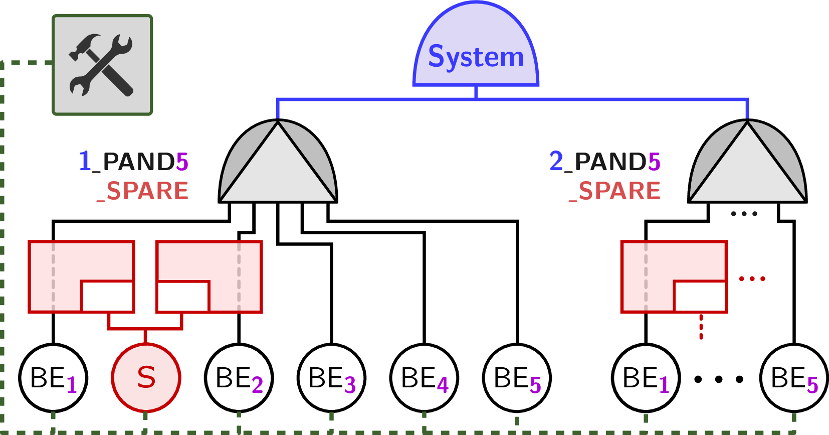
the case study from [11], with 4 \(\mathsf{\MakeUppercase{pand}}\) gates and uniform fail/repair distributions
the larger system from 5, with \(\mathsf{\MakeUppercase{and}}\), \(\mathsf{\MakeUppercase{pand}}\), and \(\mathsf{\MakeUppercase{spare}}\) gates, and Weibull, normal, and exponential fail/dormant/repair distributions.
In both models—described in full detail in 12—there is a single \(\mathsf{\MakeUppercase{rbox}}\), making all BEs and SBEs interdependent.
6.1.2 Queueing networks.↩︎
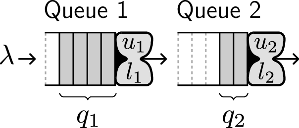
A tandem queue consists of \(n\) queues connected in series, with arrivals (departures) from outside via the first (resp.last) queue only. We experiment on the minimal \(n=2\) case from 6 (\(\mathfrak{m}_{Q}\)), with exponentially distributed inter-arrival times at rate \(\lambda\), and uniform service times at the \(i\)-th queue with \(l_i<u_i\) bounds. We study the time-bounded probability of a packet loss in the second queue due to arrivals over a limiting capacity, \(q_2\geq C\).
6.2 Experimental Setting↩︎
We study time-bounded events on each model \(\mathfrak{m}\in\{\mathfrak{m}_{\mathlarger s},\mathfrak{m}_{\ell},\mathfrak{m}_{Q}\}\): For the DFTs, we query the probability \(\varphi_{\mathfrak{m}} = P( \mathop{\mathfrak{m}}(t)\in\mathit{fail} \mid t\leq T )\) of observing a full system failure in \(\mathfrak{m}_{\mathlarger s}\)(resp.\(\mathfrak{m}_{\ell}\)) within \(T=1248\) (resp.\(4500\)) time units. For the tandem queue, we query the overflow probability \(\varphi_{\mathfrak{m}} = P(q_2\geq3\mid t\leq 11)\).
Let \({\mathfrak{a}}_\mathrm{\Phi}\) denote the use of RES algorithm \(\mathfrak{a}\) with IFUN \(\mathrm{\Phi}\). To measure the quality of (our implementation of) \(\mathrm{\Phi}\) for ISPLIT RES, we run \({\mathfrak{a}}_\mathrm{\Phi}\) with modes for 20min on each model \(\mathfrak{m}\), producing a 95% confidence interval \(\hat{\varphi}_{\mathfrak{m}}^{{\mathfrak{a}}_\mathrm{\Phi}}\) whose width \({\left|\hat{\varphi}_{\mathfrak{m}}^{{\mathfrak{a}}_\mathrm{\Phi}}\right|}\) is a quality metric of \({\mathfrak{a}}_\mathrm{\Phi}\). We normalize these values using the relative error \(\mathit{re}_{\mathfrak{m}}^{{\mathfrak{a}}_\mathrm{\Phi}} \doteq {\left(\frac{1}{2}\cdot\left|\hat{\varphi}_{\mathfrak{m}}^{{\mathfrak{a}}_\mathrm{\Phi}}\right|\right)} / {\varphi_{\mathfrak{m}}}\), where the ground truth \(\varphi_{\mathfrak{m}}\) is approximated via 12-hour-long CMC runs: A more efficient \({\mathfrak{a}}_\mathrm{\Phi}\) yields a smaller \(\mathit{re}_{\mathfrak{m}}^{{\mathfrak{a}}_\mathrm{\Phi}}\).
| IFUN | \(d_{*G}\) | \(d_*^r\) | prune | |
|---|---|---|---|---|
| \(\boldsymbol{✔}\) | ||||
| (\(d\)) | \(\boldsymbol{✔}\) | |||
| (\(d_O\)) | \(\boldsymbol{✔}\) | \(\{d_{OG}\}\) | ||
| (\(d_T\)) | \(\boldsymbol{✔}\) | \(\boldsymbol{✔}\) | \(\{d_{TG},d_{TG}^r\}\) |
r.38
Concretely, we use the RES algorithms Fixed Effort and RESTART [26], [27], selecting thresholds with lightweight Sequential Monte Carlo [28], for efforts 8 and 15 for Fixed Effort and 2 and 3 for RESTART, i.e.\(\mathfrak{a} \in \mathfrak{A}\doteq\{\textsf{\smaller[.5]FE}\ifthenelse{\equal{8}{}}{}{_{8}},\) \(\textsf{\smaller[.5]FE}\ifthenelse{\equal{15}{}}{}{_{15}},\textsf{\smaller[.5]RST}\ifthenelse{\equal{2}{}}{}{_{2}}, \textsf{\smaller[.5]RST}\ifthenelse{\equal{3}{}}{}{_{3}}\}\) [15]. We then aggregate all values per \(\ac{IFUN}\times\text{model}\) into a single scalar \(\mathit{re}_{\mathfrak{m}}^{\mathrm{\Phi}}=\mathop{\Gamma}_{\mathfrak{a\in A}}\{\mathit{re}_{\mathfrak{m}}^{{\mathfrak{a}}_\mathrm{\Phi}}\}\) that demonstrates the quality of \(\mathrm{\Phi}\) for ISPLIT. We use two aggregation functions: \(\Gamma=\mathrm{median}\) to measure expected quality, and \(\Gamma=\min\) to observe best-case possibilities. In all cases a better IFUN \(\mathrm{\Phi}\) yields a smaller \(\mathit{re}_{\mathfrak{m}}^{\mathrm{\Phi}}\).
We thus use relative errors to compare 13 IFUNs that 1 maps to the taxonomy from 3:
For the time-agnostic functions tagn_mono(the distance metric \(d\)) and tagn_comp(counting \(q_2\) for \(\mathfrak{m}_{Q}\), or a compositional IFUN for the DFTs, see 11 and [9]), we also test their resampling variants \(d_*^r\)
For the (time-sensitive) order metrics tsen_order(\(d_O\)), we also test the global-timer variant \(d_{OG}\), including a variant \(\textsf{tsen{\tt\_}order}_{\mathsf{global\mathop{\scriptscriptstyle\circ}prune}}\) that prunes the runs which provably cannot reach the target in the remaining time
For the (time-sensitive) timed metrics tsen_timed(\(d_T\)), we test all combinations of resampling, global timer, and pruning
. Since we are evaluating time-bounded queries, we do not test exact global age IFUNs (\(d_{*EG}\) in 3). We further omit experiments with some equivalent specimens from the taxonomy, e.g.\(d_O^r\) and \(d_{OG}^r\).
6.3 Experimental Results↩︎
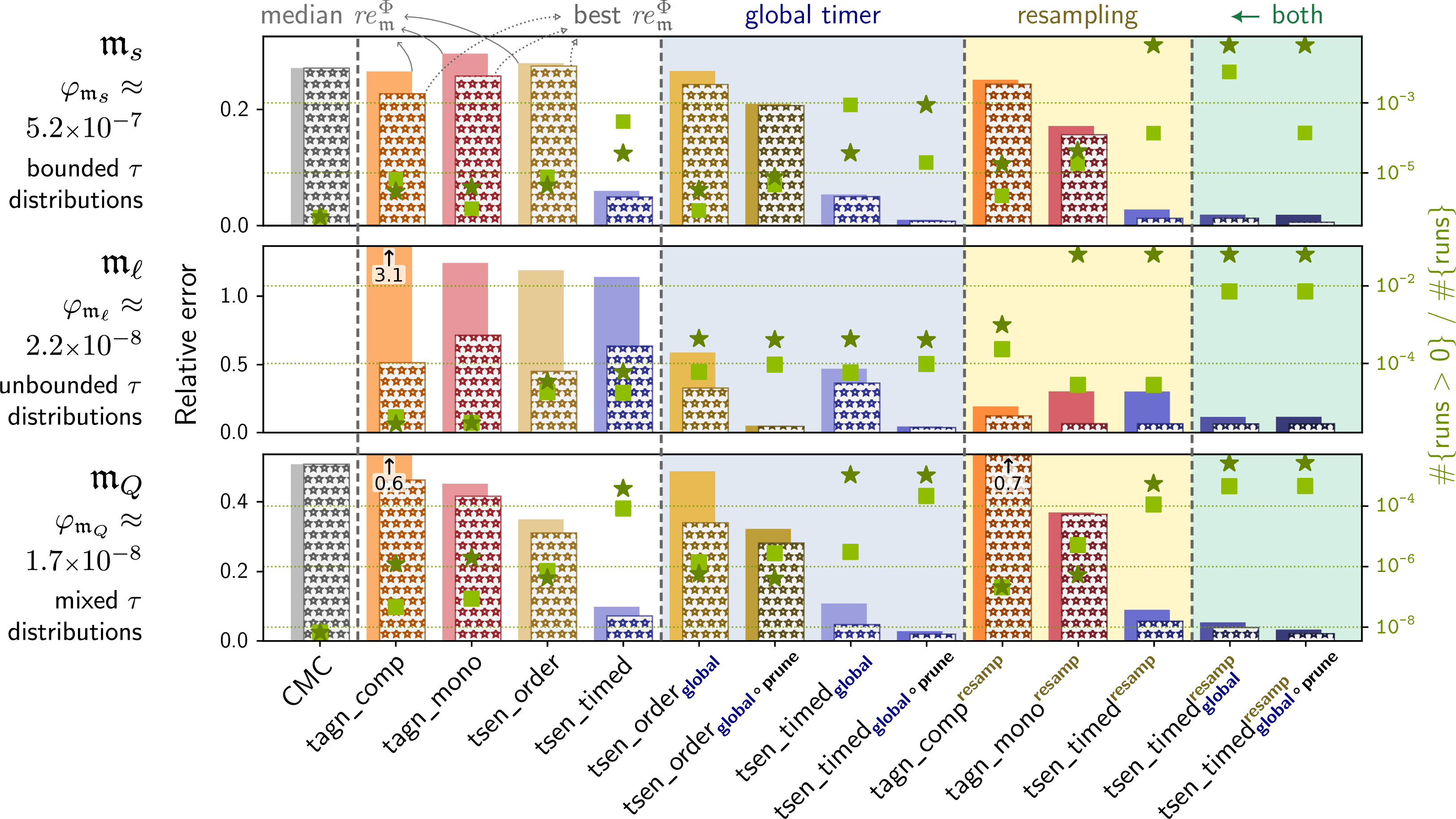
7 shows the results of our experiments, for approximated ground truths \(\varphi_{\mathfrak{m}_{\mathlarger s}}\approx5.2\scalebox{.85}{\text{\scshape e-}7}\), \(\varphi_{\mathfrak{m}_{\ell}}\approx2.2\scalebox{.85}{\text{\scshape e-}8}\), and \(\varphi_{\mathfrak{m}_{Q}}\approx1.7\scalebox{.85}{\text{\scshape e-}8}\). The height of a bar indicates the relative error achieved by each IFUN \(\mathrm{\Phi}\) and CMC: solid plain-color bars in the back stand for \(\mathrm{median}\) \(\mathit{re}_{\mathfrak{m}}^{\mathrm{\Phi}}\) values, and star-hatched bars in the front stand for \(\min\) (“best”) values. The secondary \(y\)-axis plots the proportion of “useful” runs that observed a rare event, with \(\blacksquare\) and respectively for the median and best runs. For example, for model \(\mathfrak{m}_{\ell}\) and IFUN \(\textsf{tsen{\tt\_}timed}_{\mathsf{global}}\)—the most central blue bars in the middle plot in 7—the median and best relative errors were and 0.36, with resp.proportions of useful runs of \(5.9\scalebox{.85}{\text{\scshape e-}5}\) and \(4.2\scalebox{.85}{\text{\scshape e-}4}\). [tab:experiments:results] in 12 shows the numerical results used to compile 7.
Since timers in \(\mathfrak{m}_{\mathlarger s}\) are bounded (uniform distributions), the impact of time-granularity (2) in the upper plot is apparent. Visual comparisons should be done along a single dimension of 3, e.g.either \(d_O\)vs.\(d_T\) (without global timer) or else \(d_{OG}\)vs.\(d_{TG}\). For instance, \(d_O\preceq d_T\) means that tsen_order should be less efficient than tsen_timed to estimate \(\varphi_{\mathfrak{m}_{\mathlarger s}}\), which is evidenced by the
higher bars of tsen_order in the upper plot of 7. Comparing \(\textsf{tsen{\tt\_}order}_{\mathsf{global}}\) vs.\(\textsf{tsen{\tt\_}timed}_{\mathsf{global}}\) tells the same story, and can be explained by \(d_{OG}\preceq d_{TG}\). Analogous results can be seen in the lower plot corresponding to \(\mathfrak{m}_{Q}\), where the service times also follow bounded distributions. In contrast, the unbounded timers of \(\mathfrak{m}_{\ell}\) make the difference due to time granularity much less
pronounced.
In cases like \(\mathfrak{m}_{\ell}\), where specific timer constellations must be reached in an asymmetric state space, resampling achieves the biggest performance boost. This applies to both time-agnostic and
-sensitive IFUNs to a similar degree (in compliance with 1 for models with unbounded timer domains), as evidenced by the lower bars of the \(d^r_\ast\) variants for tagn_mono,
tagn_comp, and tsen_timed in the middle plot of 7. Computational overhead also has a big impact in this (largest) model:
for both \(d_{OG}\) and \(d_{TG}\), pruning runs that cannot reach the rare event before the time limit produces narrower CIs. Note that this is purely a matter of achieving more runs in the given simulation budget, even though the proportion of useful runs generated is the same with or without pruning.
In contrast to these DFTs, queueing systems like \(\mathfrak{m}_{Q}\) have a fully connected and symmetrical state space, where resampling has a much
lower impact. However, early pruning significantly increases the number of executed runs and thus yields more accurate estimates, as we observe that \(\textsf{tsen{\tt\_}order}_{\mathsf{global\mathop{\scriptscriptstyle\circ}prune}}\) has lower relative errors than tsen_order alone, and analogously for tsen_timed.
On the representativeness of our experiments. These results demonstrate many practical implications of the taxonomy in 5, in a reduced but varied set of models. We highlight that, despite getting results that we can explain with 5, we only have a partial empirical view. For instance, to compare functions like \(\textsf{tsen{\tt\_}order}_{\mathsf{global\mathop{\scriptscriptstyle\circ}prune}}\) and \(\textsf{tsen{\tt\_}timed}^{\mathsf{resamp}}_{\mathsf{global}}\), our numerical results do not allow us to discriminate how much performance gain is due to information depth (IFUN granularity) and how much to computational overhead (resampling, pruning). A more nuanced answer to these practical questions requires a much larger experimental setup, which falls outside the scope of this contribution.
7 Conclusion↩︎
In this paper, we substantially extended the original concept of time-sensitive ISPLIT [11] by considering resampling and information about the global age. We discovered different distance metrics and explored the tradeoff between information depth and computational costs. We demonstrated the feasibility and effectiveness of our approach for a relevant class of repairable DFT models.
.7ex plus .2ex minus .1ex -.5em Limitations and future work. While the experimental evaluation demonstrated significant performance improvements compared to existing approaches, these improvements have thus far only been established experimentally. Consequently, deriving theoretical performance guarantees under a controlled setting, analogous to previous ISPLIT work [12], [13], remains an important avenue for future research. Methodically, instead of fixing a concrete time for every elapsed timer in a step (see 6), one can do this only for a subset of the elapsed timers, effectively obtaining a mixture between SSC analysis and simulation.
.7ex plus .2ex minus .1ex -.5em Data availability statement. An artifact for experimental reproduction of the results in 6 is publicly available at DOI .
.7ex plus .2ex minus .1ex -.5em Acknowledgments. We thank Pedro R. D’Argenio from Universidad Nacional de Córdoba for fruitful discussions about the relationship between time-sensitive ISPLIT and resampling.
[BE]basic element [BFS]breadth-first search [BM]Bernstein mixed polynomial and expolynomial [BP]Bernstein polynomial [CDF]cumulative distribution function [CI]confidence interval [CMC]crude Monte Carlo [CTMC]continuous-time Markov chain [DAG]directed-acyclic graph [DET]deterministic [DBM]difference bound matrix [DFT]dynamic fault tree [DKW]Dvoretzky–Kiefer–Wolfowitz [DSPN]deterministic and stochastic Petri net [DTMC]discrete-time Markov chain [EXP]exponential [ERTMS]European Rail Traffic Management System [ES]expected success [ETCS]European Train Control System [FE]fixed effort [FS]fixed success [FTA]fault tree analysis [FT]fault tree [FW]Floyd-Warshall [GEN]general [GSMP]generalized semi-Markov process [GSPN]generalized stochastic Petri net [HPnG]hybrid Petri net with general transitions [IFUN]importance function [IMM]immediate [IOSA]input/output stochastic automaton [IS]importance sampling [ISPLIT]importance splitting [JPD]joint probability distribution [MC]Monte Carlo [SMP]semi-Markov process [MRGP]Markov regenerative process [MRnP]Markov renewal process [MSE]mean-squared error [PTA]probabilistic timed automaton [PTCTL]probabilistic TCTL [PDF]probability density function [PN]Petri net [PLT]parametric location tree [RESTART]repetitive simulation trials after reaching thresholds [RES]rare event simulation [SBE]spare basic element [SC]state class [SCG]state class graph [SEQ]sequential Monte Carlo [SMC]statistical model checking [SSC]stochastic state class [STA]stochastic timed automaton [STPN]stochastic time Petri net [TA]timed automaton [TCTL]timed computation tree logic [TLE]top-level event [TPN]time Petri net [VI]value iteration [i.i.d.]independent and identically distributed [w.l.o.g.]without loss of generality [RV]random variable [LCM]least common multiple [BMs]Bernstein mixed polynomials and expolynomials [BPs]Bernstein polynomials [CIs]confidence intervals [CTMCs]continuous-time Markov chains [DAGs]directed-acyclic graphs [DBMs]difference bound matrices [DTMCs]discrete-time Markov chains [FTs]fault trees [GSPNs]generalized stochastic Petri nets [HPnGs]hybrid Petri nets with general transitions [IOSA]input/output stochastic automata [MRGPs]Markov regenerative processes [MRnPs]Markov renewal processes [PTA]probabilistic timed automata [PNs]Petri nets [RVs]random variables [SCs]state classes [SMPs]semi-Markov processes [SSCs]stochastic state classes [STA]stochastic timed automata [STPNs]stochastic time Petri nets [TA]timed automata [TLEs]top-level events [TPNs]time Petri nets
8 Backwards Reachability Calculations with State Classes↩︎
We recall the calculations of predecessor SCs in an IOSA from [11].
Target SCs. For each target location \(l'\), we build the largest possible domain \(D'\) for the active timers in \(l'\), considering only whether the target location \(l'\) is reachable from these evaluations of timers, not whether these evaluations of timers are reachable from an initial state. To this end, we limit each timer \(t_i \in T_{l'}\) by its upper bound \(b_i \in \mathbb{Q}_{\geq 0} \cup \{\infty\}\), obtaining the SC \(\Sigma' = \langle l', D'\rangle\) with \(D' = \bigtimes_{t_i \in T_{l'}} [0,b_i] \subseteq (\mathbb{Q}_{\geq 0} \cup \{\infty\})^{|T_{l'}|}\). Note that \(D'\) does not introduce dependencies between the involved timers, so \(D'\) has a hyper-rectangular shape. Conversely, we do not limit \(t_i\) by its lower bound \(a_i \in \mathbb{Q}_{\geq 0}\) given that, depending on the sequence of executed transitions, it may not be newly activated in \(l'\) (i.e., after the last incoming transition).
Predecessor SC. Given an SC \(\Sigma' = \langle l', D'\rangle\) and an incoming transition \(l\xrightarrow{{\raisebox{-1pt}[0pt][0pt]{\scriptstyle{\scriptscriptstyle T,a,T'}}}}l'\), we compute the largest possible SC \(\Sigma = \langle l, D\rangle\) such that for any state \(s\) in \(\Sigma\), the action \(a\) leads to a state \(s'\) in \(\Sigma'\) (we could say that \(\Sigma\) is the weakest precondition of \(\Sigma'\) given \(a\)). At each step of this derivation, we normalize the DBM domain of the SC being computed using the Floyd-Warshall algorithm [20] (as in forwards analysis), ensuring the uniqueness of the result and the correct resolution of all transitive restrictions. In the following derivation steps, let \(\boldsymbol{\tau}\) and \(\boldsymbol{\tau}'\) be the vectors of random variables containing the active timers in \(l\) and \(l'\), respectively:
Inverse of newly activating: Let \(\boldsymbol{\tau}' := \langle t_2', \ldots, t_{n+m}' \rangle\) and \(t_{n+1}', \ldots, t_{n+m}' \in T'\) be the \(m\) newly activated timers in \(l'\). We limit each such timer by its lower bound (as no time elapses from new activation to entrance in \(\Sigma'\)), obtaining \[\boldsymbol{\tau}_a := \langle t_2^a, ..., t_n^a, t_{n + 1}^a, ..., t_{n+m}^a \rangle = \boldsymbol{\tau}' \,\mid\, t_{n+1}', ..., t_{n+m}' \in T'\text{,}\] with support \[D_a = D' \cap \{ a_i \leq \tau(t_i')\;\forall\, i \in \{n + 1, ..., n+m\} \}\text{.}\] After normalizing \(D_a\), we remove \(t_{n+1}^a, \ldots, t_{n+m}^a\) from \(\boldsymbol{\tau}_a\), yielding \[\boldsymbol{\tau}_b := \langle t_2^b, \ldots, t_n^b \rangle = \langle t_2^a, \ldots, t_n^a \rangle\] with support: \[\begin{align} D_b &= \{ \langle \tau(t_2^a), ..., \tau(t_n^a) \rangle\\ &\qquad \text{s.t. } \exists\, \begingroup \begingroup\lccode`~=`, \lowercase{\endgroup \edef~{\mathchar\the\mathcode`, \penalty 0 \noexpand} }\mathcode`,="8000 \tau(t_{n+1}^a), ..., \tau(t_{n+m}^a) \endgroup \\ &\qquad \text{s.t. } \langle \tau(t_2^a), ..., \tau(t_n^a), \tau(t_{n+1}^a), ..., \tau(t_{n+m}^a)\rangle \in D_a \} \end{align}\]
Inverse of time advancement: We increase the timers by the timer expiring first in \(\Sigma\), say \(t_1^b\), obtaining \[\begingroup \begingroup\lccode`~=`, \lowercase{\endgroup \edef~{\mathchar\the\mathcode`, \penalty 0 \noexpand} }\mathcode`,="8000 \boldsymbol{\tau}_c := \langle t_1^{c}, \ldots, t_n^{c} \rangle = \langle t_1^b, t_2^b + t_1^b, \ldots, t_n^b+t_1^b \rangle \endgroup\] with support: \[\begin{align} D_c &= \{ \langle \tau(t_1^b), \tau(t_2^b), \ldots, \tau(t_n^b) \rangle\\ &\qquad \text{s.t. } \tau(t_1^b) \in [0, \infty) \\ &\qquad \text{s.t. } \langle \tau(t_2^b) - \tau(t_1^b), \ldots, \tau(t_n^b) - \tau(t_1^b)\rangle \in D_b\} \end{align}\]
Applying upper bounds of timers: After normalizing \(D_c\), we limit each active timer by its upper bound (to guarantee the timer does not exceed the bound due to the time retardation), obtaining \[\boldsymbol{\tau} := \langle t_1, ..., t_n\rangle = \boldsymbol{\tau}_c \,\mid\; t_i^c \leq b_i \;\forall\, i \in \{1, ..., n\}\] with the final domain (which is finally normalized, similarly to the previous passages): \[D = D_c \cap \{\tau(t_i^c) \leq b_i\;\forall\, i \in \{1, ..., n\}\}\]
Note that there is no need for a conditioning step to guarantee that the timer \(t_1^b\) expiring first actually elapses before the other timers. In fact, the non-negativity of the timer evaluations in domain \(D_b\), i.e., \(0\leq \tau(t^b_i) - \tau(t^b_1)\) \(\forall\,i\in\{2, ..., n\}\), already implies that \(\tau(t^b_1) \leq \tau(t^b_i)\) \(\forall\,i\in\{2, ..., n\}\).
Disabled timers. As mentioned in 2.1, there are cases occurring in the repairable DFT semantics in [19], although not strictly being part of the original IOSA definition, where a set of timers, say \(t_2, ..., t_{p+1} \in T_d\), is disabled while taking a transition. In this case, only the elapsing timer was added in step [en:sc-step2] (inverse of time advancement). Thus, we need to insert the \(p\) disabled timers \(t_2, ..., t_{p+1}\) after step [en:sc-step2] into the zone \(D_c\) while ensuring that these elapse after \(t_1\). Formally, we expand the set of timers \(\boldsymbol{\tau}_c = \langle t_1^c, t_{p+2}^c, ..., t_n^c\rangle\), obtaining \[\begingroup \begingroup\lccode`~=`, \lowercase{\endgroup \edef~{\mathchar\the\mathcode`, \penalty 0 \noexpand} }\mathcode`,="8000 \boldsymbol{\tau}_d := \langle t_1^{d}, t_2^{d}, \ldots, t_n^{d} \rangle = \langle t_1^c, t_2, \ldots, t_{p+1}, t_{p+2}^c, \ldots, t_n^c \rangle \endgroup\] with support: \[\begin{align} D_d &= \{ \langle \tau(t_1^d), \tau(t_2^d), \ldots, \tau(t_n^d) \rangle\\ &\qquad \text{s.t. } \forall\,i\in \{2, ..., p+1\} : \tau(t_i^d) \in [0, \infty) \wedge \tau(t_1^d) \leq \tau(t_i^d) \\ &\qquad \text{s.t. } \langle \tau(t_1^d), \tau(t_{p+2}^d), \ldots, \tau(t_n^d)\rangle \in D_c\} \end{align}\] In step [en:sc-step3] (applying upper bounds of timers), we then have to work with \(\boldsymbol{\tau}_d\) instead of \(\boldsymbol{\tau}_c\) and \(D_d\) instead of \(D_c\), respectively.
9 Resampling Implementation↩︎
As each timer can be resampled individually, we solely have to answer how to sample from a truncated timer distribution. Formally, for a timer \(t_i\), let \(X_i\) be the random variable distributed according to the CDF \(F_i\). Analogously, let \(Y_i = (X_i \mid X_i \geq \tau_{\textit{elp}}(t_i)) - \tau_{\textit{elp}}(t_i)\) be the random variable that is based on \(X_i\), but truncates all values below \(\tau_{\textit{elp}}(t_i)\) and subtracts the elapsed time. Sampling of \(Y_i\) corresponds to resampling the value of timer \(t_i\). Exponential distributions can be resampled without adaptations due to the memoryless property as it holds here that \(X_i = Y_i\). Furthermore, for the case \(\tau_{\textit{elp}}(t_i) \leq a_i\), it holds \((X_i \mid X_i \geq \tau_{\textit{elp}}(t_i)) = X_i\), so we can sample from the distribution \(X_i\) and subtract the elapsed time \(\tau_{\textit{elp}}(t_i)\) to obtain a sample from \(Y_i\). Otherwise, as in [9], we distinguish two cases:
For distributions where the inverse CDF \(F_i^{-1}\colon [0,1]\rightarrow \mathbb{R}_{\geq0}\) exists or can be approximated efficiently (e.g., Uniform, Normal, or Rayleigh distribution), we can compute a sample for \((X_i \mid X_i \geq \tau_{\textit{elp}}(t_i))\) via inverse transform sampling as follows: First, create a random value \(u\sim \mathrm{\small Unif}[0,1]\), and then create a sample for \((X_i \mid X_i \geq \tau_{\textit{elp}}(t_i))\) by evaluating \(F^{-1}(u + (1 - u)\cdot F(\tau_{\textit{elp}}(t_i)))\).
Otherwise (e.g., Erlang or Weibull distribution), we evaluate \((X_i \mid X_i \geq \tau_{\textit{elp}}(t_i))\) by rejection sampling, i.e., sample values of \(X_i\) until one is at least \(\tau_{\textit{elp}}(t_i)\) and then calculate \(Y_i\). To limit the computational complexity beforehand, we fix a maximum number of sampling attempts (in our case \(k = 20\)) and resort to the old value \(X_i\) if no suitable sample has been found.
Note that limiting the number of sampling attempts to \(k\) retains the old sample with a probability of \(F(\tau_{\textit{elp}}(t_i))^k\) instead of creating a new one. Although the old sample is used, the timer evaluation still represents an unbiased sample from the conditioned distribution \((X_i \mid X_i \geq \tau_{\textit{elp}}(t_i))\) and does ultimately yield unbiased simulation results: As a time of \(\tau_{\textit{elp}}(t_i)\) has elapsed for timer \(t_i\), the old sampled timer value is distributed according to \((X_i \mid X_i \geq \tau_{\textit{elp}}(t_i))\). Furthermore, the probability that the old sample is retained is independent of the old sampled timer value.
10 Omitted Proofs↩︎
1. Remember that \(\omega(l)\) (distance of each location to the target) is calculated by backwards reachability search from the target states. Consider a state \(s = \langle l, \tau\rangle\). First, we show that, for each state \(s\), the distance \(d(s)\) is an upper bound of the ordered distance with resampling \(d_O^r(s)\). Specifically, let \(\omega(l)=n\). By definition of backwards reachability, there exists a shortest sequence of actions and locations \(l_n \stackrel{a_n}{\rightarrow} l_{n-1} \stackrel{a_{n-1}}{\rightarrow} l_{n-2} \stackrel{a_{n-2}}{\rightarrow} \dots \stackrel{a_1}{\rightarrow} l_0\) such that \(l_n=l\), \(l_0\) is a target location, and \(\omega(l_i)=i\) for all \(i\in \{0, ..., n\}\). Then, we consider the corresponding sequence of elementary SCs \(\Sigma_n \stackrel{a_n}{\rightarrow} \Sigma_{n-1} \stackrel{a_{n-1}}{\rightarrow} \Sigma_{n-2} \stackrel{a_{n-2}}{\rightarrow} \dots \stackrel{a_1}{\rightarrow} \Sigma_0\) with \(\omega_O(\Sigma_i) = i\) for \(i\in \{0, ..., n\}\). Given that all timers are unbounded, no timer is disabled due to clock bounds. Consequently, a valid execution sequence matching the sequence of actions and locations is guaranteed to exist, implying that \(\omega_O(\Sigma_n)\leq n\). Since \(\omega(l)\) represents the shortest distance unconstrained by timer values, \(\omega_O(\Sigma_n)\) cannot be strictly lower than \(n\), implying that there exists an elementary SC \(\Sigma_{\sigma}\) s.t. \(\omega(l) = \omega_O(\Sigma_{\sigma})\).
Second, via resampling, independent of the elapsed time \(\tau_{\textit{elp}}\), the induced SC \(\Sigma_{s_{\textit{elp}}}\) always intersects with any of the \(|T_l|!\) elementary SCs of location \(l\). For reference, consider any timer permutation \(\sigma\). Define \(\tau = \{\sigma(t_1) \mapsto 1, \sigma(t_2) \mapsto 2, ..., \sigma(t_n) \mapsto n \}\). Then, \(\tau\) is both contained in \(\Sigma_{\sigma}\) (the order of the timer values is trivially given) and \(\Sigma_{s_{\textit{elp}}}\) (the lower bound is always zero, and no upper bound exists as we are solely working with unbounded timers), so \(\Sigma_{\sigma}\) and \(\Sigma_{s_{\textit{elp}}}\) intersect.
Combining both arguments, it follows directly that \(d(s) = d^r_O(s)\) for \(s\in\mathcal{S}\). ◻
2. We prove the statements individually:
\(d \equiv d^r_{O} \equiv d^r_{OG} \equiv d^r_{OEG}\) (Equivalence for order with resampling)
\(d \equiv d^r_{O}\) was already proven by 1. Consider \(d^r_{O} \equiv d^r_{OG}\). For a state \(s\) and distance metric \(d^r_O\), we have a look at the shortest possible sequence of elementary SCs to the target \(\Sigma_n \stackrel{a_n}{\rightarrow} \Sigma_{n-1} \stackrel{a_{n-1}}{\rightarrow} \Sigma_{n-2} \stackrel{a_{n-2}}{\rightarrow} \dots \stackrel{a_1}{\rightarrow} \Sigma_0\) with \(\omega_O(\Sigma_i) = i\) for \(i\in \{0, ..., n\}\) and delays \(\Delta_i \in \mathbb{R}_{\geq{0}}\) for \(i\in \{1, ..., n\}\). The same sequence is possible for \(d^r_{OG}\) independent of the remaining (positive) time budget \(\tau(t_\textit{age})\): Due to resampling and the unbounded distributions, one can scale the values of the sampled timers s.t. the time to execute all transitions is shorter than the remaining time budget, i.e. \(\sum_{i=1}^{n} \Delta_i \leq \tau(t_\textit{age})\), while preserving the order of timers in each state. This makes the same sequence possible as for \(d^r_{O}\). Similarly to the argument made in 1, no shorter sequence exists, proving \(d^r_{O} \equiv d^r_{OG}\). To prove \(d^r_{OG} \equiv d^r_{OEG}\), one recognizes that a simulation run can always stay in a target state infinitely long (as no upper bounds on the timers exist), so it only matters that a target state is reached within the given time limit (and so \(d^r_{OG}\) and \(d^r_{OEG}\) coincide here).\(d_O \preceq d_{OG} \preceq d_{OEG}\), \(d_T \preceq d_{TG} \preceq d_{TEG}\), \(d^r_T \preceq d^r_{TG} \preceq d^r_{TEG}\) (Age inclusion)
\(d \preceq d_O\), \(d_O \preceq d_T\), \(d_{OG} \preceq d_{TG}\), \(d_{OEG} \preceq d_{TEG}\), \(d \preceq d^r_T\) (Time granularity)
All of these statements from [en:thm2-2]. and [en:thm2-3]. of the type \(d_A \preceq d_B\) follow directly from the fact that the left side \(d_A\) applies strictly fewer restrictions than the right side \(d_B\). Thus, every sequence of states to the target \(s_n \stackrel{a_n}{\rightarrow} s_{n-1} \stackrel{a_{n-1}}{\rightarrow} s_{n-2} \stackrel{a_{n-2}}{\rightarrow} \dots \stackrel{a_1}{\rightarrow} s_0\) reflected by \(d_A\) cannot be done in fewer steps when resorting to the restrictions denoted in the distance metric \(d_B\). For \(d \preceq d^r_T\) note that, as \(d\equiv d^r_O\) (see [en:thm2-1].), this statement is equivalent to \(d^r_O \preceq d^r_T\) and is handled by the same argument (strictly fewer restrictions) as the other statements.\(d^r_T \preceq d_T\), \(d^r_{TG} \preceq d_{TG}\), \(d^r_{TEG} \preceq d_{TEG}\) (Resampling yes/no)
We recall that 8 defines \(d^{r}_{T}(s) = \min_{s'\in \Sigma_{s_\textit{elp}}} d_{T}(s')\). Thus, it holds for every state \(s \in \Sigma_{s_\textit{elp}}\) that \(d^{r}_{T}(s) \leq d_{T}(s)\). As this is true for every elapsed time information \(s_\textit{elp}\), \(d^{r}_{T}(s) \leq d_{T}(s)\) for all \(s\in \mathcal{S}\) and thus \(d^r_T \preceq d_T\). The proof is analogous for \(d^r_{TG} \preceq d_{TG}\) and \(d^r_{TEG} \preceq d_{TEG}\).
◻
11 Time-Agnostic Compositional Importance Function Definition for Repairable Dynamic Fault Trees↩︎
¿tbl:tab:comp-ifun-def? depicts the compositional IFUN definition for repairable DFTs according to [9]. It specifies for each gate a local IFUN; for BEs and SBEs this is either \(0\) or \(1\), depending on whether the BE/SBE is working or not, while the other gates take the values of their children into account. \(\boldsymbol{z}_v\) denotes if a gate has failed, while \(\boldsymbol{x}_v\) refers to the internal state of the gate (for more details, see [9]). The weights of the children are balanced by their maximum importance; the LCM is used to attain solely integer levels despite the balancing. The local IFUN of the topmost gate resembles the global IFUN. During simulation, the global IFUN is evaluated by stepwise applying these rules until arriving at BEs or SBEs.
12 More Details About the Experiments↩︎
12.1 Theoretical Models↩︎

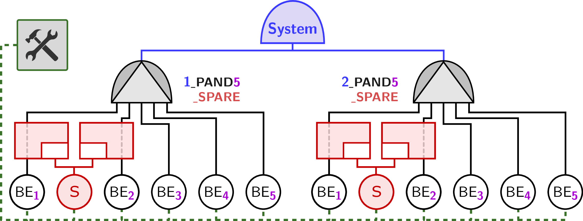
Figure 8: DFT experimentation models from 6. a — [11], b — , where \(n\)-ary \(\mathsf{\MakeUppercase{pand}}\)s are actually cascaded as in 8 (a)
This section provides more details about the models used for experiments in 6. For DFTs we study the time-bounded probability \(\varphi_{\mathfrak{m}} = P( \mathop{\mathfrak{m}}(t)\in\mathit{fail} \mid t\leq T )\) of observing a full system failure, using \(T=1248\) for \(\mathfrak{m}_{\mathlarger s}\) and \(T=4500\) for \(\mathfrak{m}_{\ell}\). The corresponding ground truth failure probabilities—approximated with 12-hours-long CMC runs—are \(\varphi_{\mathfrak{m}_{\mathlarger s}}\approx5.2\scalebox{.85}{\text{\scshape e-}7}\) and \(\varphi_{\mathfrak{m}_{\ell}}\approx2.2\scalebox{.85}{\text{\scshape e-}8}\).
All timers that govern failures and repairs in the BEs of \(\mathfrak{m}_{\mathlarger s}\) have (bounded) uniform distributions—the concrete bounds can be found in [code:modelSmall] and [11]. In contrast, \(\mathfrak{m}_{\ell}\) is sketched in 8 (b), and has basic elements whose failure, repair, and dormant-failure events obey \(\mathop{\mathit{exponential}}({\lambda}\raisebox{1pt}{\scriptstyle\,=\,}{2\cdot 10^{-4}})\), \(\mathop{\mathit{normal}}({\mu}\raisebox{1pt}{\scriptstyle\,=\,}{500},{\sigma}\raisebox{1pt}{\scriptstyle\,=\,}{50})\), and \(\mathop{\mathit{Weibull}}({\alpha}\raisebox{1pt}{\scriptstyle\,=\,}{5.6}, {\beta}\raisebox{1pt}{\scriptstyle\,=\,}{10^4})\) distributions in time, resp. Moreover, all BEs and SBEs are repaired by a single \(\mathsf{\MakeUppercase{rbox}}\), which makes all components dependent on each other. Finally, note that while \(n\)-ary \(\mathsf{\MakeUppercase{pand}}\)s are represented compactly in [fig:modelLarge,fig:experiments:models:modelLarge], they are implemented as right-cascading binary \(\mathsf{\MakeUppercase{pand}}\)s equivalently to what is shown in 8 (a), i.e.\(\mathsf{\MakeUppercase{pand}}(a,b,c)\) becomes \(\mathsf{\MakeUppercase{pand}}(a,\mathsf{\MakeUppercase{pand}}(b,c))\). Both models are described in 12.2 in a domain-specific language for DFTs.
Besides fault trees, we experiment with a classic RES benchmark from the domain of queueing networks: the two-station tandem queue. We study the time-bounded probability \(\varphi_{\mathfrak{m}_{Q}} = P(q_2\geq3\mid t\leq 11)\) of observing an overflow in the second station, whose approximated ground truth value is \(\varphi_{\mathfrak{m}_{Q}}\approx1.7\scalebox{.85}{\text{\scshape e-}8}\).
The tandem queue under consideration has mixed timers: external arrivals to the first station are governed by an (unbounded) \(\mathop{\mathit{exponential}}({\lambda}\raisebox{1pt}{\scriptstyle\,=\,}{0.17})\) distribution, while service times at the stations are governed by bounded distributions: \(\mathit{uniform}({l_1}\raisebox{1pt}{\scriptstyle\,=\,}{2},{u_1}\raisebox{1pt}{\scriptstyle\,=\,}{3})\) in the first station and \(\mathit{uniform}({l_2}\raisebox{1pt}{\scriptstyle\,=\,}{1},{u_2}\raisebox{1pt}{\scriptstyle\,=\,}{3})\) in the second. These timers were chosen such that the loads at subsequent stations are decremental. Together with the tight time bound (\(t\leq 11\)), this makes the probability \(\varphi_{\mathfrak{m}_{Q}}\) a rare event that becomes exponentially more rare with the limiting capacity \(C\) of the second queue whose overflow we are interested in measuring. The Modest model used in our experiments is introduced as [code:modelTandemQueueSA] in 12.2.
12.2 Models in Kepler/Modest Syntax↩︎
Below we provide the description of both DFT models in Kepler [9], an adaptation of the well-known Galileo input format for fault trees [32]. Kepler allows specifying general (i.e.non-Markovian) distributions for failure, repair, and dormant-failure events of BEs and SBEs.
toplevel "PAND1";
"PAND1" pand "BE1" "PAND2";
"PAND2" pand "BE2" "PAND3";
"PAND3" pand "BE3" "BE4";
"BE1" fail`\dist`uniform(1198,1218) repair`\dist`uniform(10,15);
"BE2" fail`\dist`uniform(530,595)   repair`\dist`uniform(10,45);
"BE3" fail`\dist`uniform(385,465)   repair`\dist`uniform(10,45);
"BE4" fail`\dist`uniform(1105,1205) repair`\dist`uniform(10,15);
"RBOX" rbox prio "BE1" "BE2" "BE3" "BE4";
toplevel "System";
"System" and "G1_PAND5_a" "G2_PAND5_a";
"G1_PAND5_a" pand "G1_SPARE_a" "G1_PAND5_b";
"G1_PAND5_b" pand "G1_SPARE_b" "G1_PAND5_c";
"G1_PAND5_c" pand "G1_BE_c" "G1_PAND5_d";
"G1_PAND5_d" pand "G1_BE_d" "G1_BE_e";
"G1_SPARE_a" spare "G1_BE_a" "G1_SBE";
"G1_SPARE_b" spare "G1_BE_b" "G1_SBE";
"G1_BE_a" fail`\dist`exponential(^2e-4^) repair`\dist`normal(^500^,^50^);
"G1_BE_b" fail`\dist`exponential(^2e-4^) repair`\dist`normal(^500^,^50^);
"G1_BE_c" fail`\dist`exponential(^2e-4^) repair`\dist`normal(^500^,^50^);
"G1_BE_d" fail`\dist`exponential(^2e-4^) repair`\dist`normal(^500^,^50^);
"G1_BE_e" fail`\dist`exponential(^2e-4^) repair`\dist`normal(^500^,^50^);
"G1_SBE" fail`\dist`exponential(^2e-4^) repair`\dist`normal(^500^,^50^) dorm`\dist`weibull(^5.6^,^1e4^);
"G2_PAND5_a" pand "G2_SPARE_a" "G2_PAND5_b";
"G2_PAND5_b" pand "G2_SPARE_b" "G2_PAND5_c";
"G2_PAND5_c" pand "G2_BE_c" "G2_PAND5_d";
"G2_PAND5_d" pand "G2_BE_d" "G2_BE_e";
"G2_SPARE_a" spare "G2_BE_a" "G2_SBE";
"G2_SPARE_b" spare "G2_BE_b" "G2_SBE";
"G2_BE_a" fail`\dist`exponential(^2e-4^) repair`\dist`normal(^500^,^50^);
"G2_BE_b" fail`\dist`exponential(^2e-4^) repair`\dist`normal(^500^,^50^);
"G2_BE_c" fail`\dist`exponential(^2e-4^) repair`\dist`normal(^500^,^50^);
"G2_BE_d" fail`\dist`exponential(^2e-4^) repair`\dist`normal(^500^,^50^);
"G2_BE_e" fail`\dist`exponential(^2e-4^) repair`\dist`normal(^500^,^50^);
"G2_SBE" fail`\dist`exponential(^2e-4^) repair`\dist`normal(^500^,^50^) dorm`\dist`weibull(^5.6^,^1e4^);
"RBOX" rbox prio "G2_SBE" "G2_BE_e" "G2_BE_d" "G2_BE_c" "G2_BE_b" "G2_BE_a"
"G1_SBE" "G1_BE_e" "G1_BE_d" "G1_BE_c" "G1_BE_b" "G1_BE_a";Furthermore, we provide in the following the description of the tandem queue in the Modest model description language [31]:
// Actions
action arrival, queue1_service, queue2_service, overflow;

// Constants
const int C = 3; // Capacity of each queue
const int B = 11; // Time§{\color{green!33!black}-}§bound
const real l = 0.17; // Arrival rate

// Bounds for service distribution
const real lowb1 = 2.0, uppb1 = 3.0; // of first server
const real lowb2 = 1.0, uppb2 = 3.0; // of second server

// Discrete variables and timers
int(0..C) §${\color{teal!67!black}q_1}$§, §${\color{teal!67!black}q_2}$§;
bool failed = false;
timer t_arrivals = Exponential(l), t_server_1, t_server_2;

// Ad§{\color{green!33!black}-}§hoc importance function and time§{\color{green!33!black}-}§bounded failure property
property Importance = §${\color{teal!67!black}q_2}$§;
property TimeBounded = Pmax(<>[T<=B] (failed));

// Main loop
do {
// Logic for arrivals
:: when(t_arrivals <= 0) invariant(t_arrivals >= 0) arrival
   {= t_arrivals = Exponential(l), §${\color{teal!67!black}q_1}$§ = min(§${\color{teal!67!black}q_1}$§ + 1, C),
      t_server_1 = (§${\color{teal!67!black}q_1}$§ == 0) ? Uniform(lowb1,uppb1) : t_server_1 =}
// Logic for server 1 (without triggering an overflow)
:: when(§${\color{teal!67!black}q_1}$§ > 0 && §${\color{teal!67!black}q_2}$§ < C - 1 && t_server_1 <= 0)
   invariant(§${\color{teal!67!black}q_1}$§ == 0 || §${\color{teal!67!black}q_2}$§ >= C - 1 || t_server_1 >= 0) queue1_service
   {= §${\color{teal!67!black}q_1}$§--, §${\color{teal!67!black}q_2}$§ = min(§${\color{teal!67!black}q_2}$§ + 1, C),
      t_server_1 = (§${\color{teal!67!black}q_1}$§ >  1) ? Uniform(lowb1,uppb1) : t_server_1,
      t_server_2 = (§${\color{teal!67!black}q_2}$§ == 0) ? Uniform(lowb2,uppb2) : t_server_2 =}
// Logic for server 2
:: when(§${\color{teal!67!black}q_2}$§ > 0 && t_server_2 <= 0)
   invariant(§${\color{teal!67!black}q_2}$§ == 0 || t_server_2 >= 0) queue2_service
   {= §${\color{teal!67!black}q_2}$§--, t_server_2 = §${\color{teal!67!black}q_2}$§ > 1 ? Uniform(lowb2,uppb2) : t_server_2 =}
// Check for overflow (triggered by server 1 when server 2 is full)
:: when(§${\color{teal!67!black}q_1}$§ > 0 && §${\color{teal!67!black}q_2}$§ >= C - 1 && t_server_1 <= 0)
   invariant(§${\color{teal!67!black}q_1}$§ == 0 || §${\color{teal!67!black}q_2}$§ < C - 1 || t_server_1 >= 0)
   overflow {= failed = true =}; Overflow()
}

// Failure location: we stop here
process Overflow()
{
    stop
}
12.3 Importance Functions↩︎
[code:IFUNsSmall]/[code:IFUNsLarge] show the IFUNs used for \(\mathfrak{m}_{\mathlarger s}\)/\(\mathfrak{m}_{\ell}\), matching the Kepler syntax identifiers from [code:modelSmall]/[code:modelLarge] and their corresponding IOSA translations implemented in the modes tool.
For \(\mathfrak{m}_{\mathlarger s}\), we limit the maximum expansion depth for each distance metric to \(12\). However, this still ensures that the relevant state space is covered (see detailed discussion in 12.4). For \(\mathfrak{m}_{\ell}\), we notice that the system consists of two subtrees that are solely connected by a repair box. To limit the explored state space, we construct for each subtree a local IFUN and sum up their individual IFUNs. Note that the maximum expansion depth of \(17\) for the distance metrics in \(\mathfrak{m}_{\ell}\) is chosen large enough such that the complete SC graphs are constructed.
"tagn_comp"  // IFUN time-agnostic compositional
  max(((4*E([BE1:[BE1__failure,BE1__repairing]]))+(if E([PAND1:[PAND1__first_failed,PAND1__gate_failure,PAND1__gate_repaired_first_fail,PAND1__failed_first_up,PAND1__failed_first_fail]]) then max(((2*E([BE2:[BE2__failure,BE2__repairing]]))+(if E([PAND2:[PAND2__first_failed,PAND2__gate_failure,PAND2__gate_repaired_first_fail,PAND2__failed_first_up,PAND2__failed_first_fail]]) then max((E([BE3:[BE3__failure,BE3__repairing]])+(if E([PAND3:[PAND3__first_failed,PAND3__gate_failure,PAND3__gate_repaired_first_fail,PAND3__failed_first_up,PAND3__failed_first_fail]]) then E([BE4:[BE4__failure,BE4__repairing]]) else -E([BE4:[BE4__failure,BE4__repairing]]))), if E([PAND3:[PAND3__failed_first_up,PAND3__failed_first_fail]]) then 2 else 0) else -max((E([BE3:[BE3__failure,BE3__repairing]])+(if E([PAND3:[PAND3__first_failed,PAND3__gate_failure,PAND3__gate_repaired_first_fail,PAND3__failed_first_up,PAND3__failed_first_fail]]) then E([BE4:[BE4__failure,BE4__repairing]]) else -E([BE4:[BE4__failure,BE4__repairing]]))), if E([PAND3:[PAND3__failed_first_up,PAND3__failed_first_fail]]) then 2 else 0))), if E([PAND2:[PAND2__failed_first_up,PAND2__failed_first_fail]]) then 4 else 0) else -max(((2*E([BE2:[BE2__failure,BE2__repairing]]))+(if E([PAND2:[PAND2__first_failed,PAND2__gate_failure,PAND2__gate_repaired_first_fail,PAND2__failed_first_up,PAND2__failed_first_fail]]) then max((E([BE3:[BE3__failure,BE3__repairing]])+(if E([PAND3:[PAND3__first_failed,PAND3__gate_failure,PAND3__gate_repaired_first_fail,PAND3__failed_first_up,PAND3__failed_first_fail]]) then E([BE4:[BE4__failure,BE4__repairing]]) else -E([BE4:[BE4__failure,BE4__repairing]]))), if E([PAND3:[PAND3__failed_first_up,PAND3__failed_first_fail]]) then 2 else 0) else -max((E([BE3:[BE3__failure,BE3__repairing]])+(if E([PAND3:[PAND3__first_failed,PAND3__gate_failure,PAND3__gate_repaired_first_fail,PAND3__failed_first_up,PAND3__failed_first_fail]]) then E([BE4:[BE4__failure,BE4__repairing]]) else -E([BE4:[BE4__failure,BE4__repairing]]))), if E([PAND3:[PAND3__failed_first_up,PAND3__failed_first_fail]]) then 2 else 0))), if E([PAND2:[PAND2__failed_first_up,PAND2__failed_first_fail]]) then 4 else 0))), if E([PAND1:[PAND1__failed_first_up,PAND1__failed_first_fail]]) then 8 else 0)
"tagn_mono"      // IFUN time-agnostic monolithic
  12-D([BE3,PAND1,RBOX,BE2,PAND3,PAND2,BE1,BE4],[PAND1:[PAND1__failed_first_fail]],12)
"tsen_order"     // IFUN time-sensitive order
  12-OD([BE3,PAND1,RBOX,BE2,PAND3,PAND2,BE1,BE4],[PAND1:[PAND1__failed_first_fail]],12)
"tsen_order`${}_{\mathtt{global}\!}$`" // IFUN time-sensitive order global
  12-OGD([BE3,PAND1,RBOX,BE2,PAND3,PAND2,BE1,BE4],[PAND1:[PAND1__failed_first_fail]],12)
"tsen_timed"     // IFUN time-sensitive timed
  12-TD([BE3,PAND1,RBOX,BE2,PAND3,PAND2,BE1,BE4],[PAND1:[PAND1__failed_first_fail]],12)
"tsen_timed`${}_{\mathtt{global}\!}$`" // IFUN time-sensitive timed global
  12-TGD([BE3,PAND1,RBOX,BE2,PAND3,PAND2,BE1,BE4],[PAND1:[PAND1__failed_first_fail]],12)
"tagn_comp" // IFUN time-agnostic compositional
// Omitted due to excessive length
"tagn_mono" // IFUN time-agnostic monolithic
17-D([G1_BE_e,G1_BE_a,G1_BE_c,G1_SBE,G1_BE_b,G1_SBE__multiplexer,G1_PAND5_d,G1_SPARE_b,G1_PAND5_a,RBOX,G1_PAND5_c,G1_BE_d,G1_SPARE_a,G1_PAND5_b],[G1_PAND5_a:[G1_PAND5_a__failed_first_fail]],17)+17-D([G2_SBE,G2_SBE__multiplexer,G2_BE_a,G2_BE_b,G2_BE_e,G2_PAND5_c,G2_SPARE_a,RBOX,G2_BE_d,G2_BE_c,G2_PAND5_b,G2_PAND5_a,G2_PAND5_d,G2_SPARE_b],[G2_PAND5_a:[G2_PAND5_a__failed_first_fail]],17)
"tsen_order" // IFUN time-sensitive order
17-OD([G1_BE_e,G1_BE_a,G1_BE_c,G1_SBE,G1_BE_b,G1_SBE__multiplexer,G1_PAND5_d,G1_SPARE_b,G1_PAND5_a,RBOX,G1_PAND5_c,G1_BE_d,G1_SPARE_a,G1_PAND5_b],[G1_PAND5_a:[G1_PAND5_a__failed_first_fail]],17)+17-OD([G2_SBE,G2_SBE__multiplexer,G2_BE_a,G2_BE_b,G2_BE_e,G2_PAND5_c,G2_SPARE_a,RBOX,G2_BE_d,G2_BE_c,G2_PAND5_b,G2_PAND5_a,G2_PAND5_d,G2_SPARE_b],[G2_PAND5_a:[G2_PAND5_a__failed_first_fail]],17)
"tsen_order`${}_{\mathtt{global}\!}$`" // IFUN time-sensitive order global
17-OGD([G1_BE_e,G1_BE_a,G1_BE_c,G1_SBE,G1_BE_b,G1_SBE__multiplexer,G1_PAND5_d,G1_SPARE_b,G1_PAND5_a,RBOX,G1_PAND5_c,G1_BE_d,G1_SPARE_a,G1_PAND5_b],[G1_PAND5_a:[G1_PAND5_a__failed_first_fail]],17)+17-OGD([G2_SBE,G2_SBE__multiplexer,G2_BE_a,G2_BE_b,G2_BE_e,G2_PAND5_c,G2_SPARE_a,RBOX,G2_BE_d,G2_BE_c,G2_PAND5_b,G2_PAND5_a,G2_PAND5_d,G2_SPARE_b],[G2_PAND5_a:[G2_PAND5_a__failed_first_fail]],17)
"tsen_timed" // IFUN time-sensitive timed
17-TD([G1_BE_e,G1_BE_a,G1_BE_c,G1_SBE,G1_BE_b,G1_SBE__multiplexer,G1_PAND5_d,G1_SPARE_b,G1_PAND5_a,RBOX,G1_PAND5_c,G1_BE_d,G1_SPARE_a,G1_PAND5_b],[G1_PAND5_a:[G1_PAND5_a__failed_first_fail]],17)+17-TD([G2_SBE,G2_SBE__multiplexer,G2_BE_a,G2_BE_b,G2_BE_e,G2_PAND5_c,G2_SPARE_a,RBOX,G2_BE_d,G2_BE_c,G2_PAND5_b,G2_PAND5_a,G2_PAND5_d,G2_SPARE_b],[G2_PAND5_a:[G2_PAND5_a__failed_first_fail]],17)
"tsen_timed`${}_{\mathtt{global}\!}$`" // IFUN time-sensitive timed global
17-TGD([G1_BE_e,G1_BE_a,G1_BE_c,G1_SBE,G1_BE_b,G1_SBE__multiplexer,G1_PAND5_d,G1_SPARE_b,G1_PAND5_a,RBOX,G1_PAND5_c,G1_BE_d,G1_SPARE_a,G1_PAND5_b],[G1_PAND5_a:[G1_PAND5_a__failed_first_fail]],17)+17-TGD([G2_SBE,G2_SBE__multiplexer,G2_BE_a,G2_BE_b,G2_BE_e,G2_PAND5_c,G2_SPARE_a,RBOX,G2_BE_d,G2_BE_c,G2_PAND5_b,G2_PAND5_a,G2_PAND5_d,G2_SPARE_b],[G2_PAND5_a:[G2_PAND5_a__failed_first_fail]],17)[code:IFUNsQueue] shows the IFUNs used for the tandem queue model \(\mathfrak{m}_{Q}\) from [code:modelTandemQueueSA]. Note that loc_20 refers to the failure location
(i.e., an overflow happened) of the model. Again, the maximum expansion depth of \(30\) ensures that the complete SC graph is constructed.
"tagn_comp"  // IFUN time-agnostic compositional
  // Encoded in the Modest code in property `\texttt{Importance}`
"tagn_mono"      // IFUN time-agnostic monolithic
  30-D([Main], [Main:[loc_20]], 30)
"tsen_order"     // IFUN time-sensitive order
  30-OD([Main], [Main:[loc_20]], 30)
"tsen_order`${}_{\mathtt{global}\!}$`" // IFUN time-sensitive order global
  30-OGD([Main], [Main:[loc_20]], 30)
"tsen_timed"     // IFUN time-sensitive timed
  30-TD([Main], [Main:[loc_20]], 30)
"tsen_timed`${}_{\mathtt{global}\!}$`" // IFUN time-sensitive timed global
  30-TGD([Main], [Main:[loc_20]], 30)
12.4 Construction Times of Importance Functions↩︎
We report on the construction times that were necessary to construct the IFUNs used during experimentation:
Fault tree \(\mathfrak{m}_{\mathlarger s}\): The construction of the complete SC graph is possible for the ordered distance metric \(\omega_O(\Sigma)\) and the timed distance metrics with global age (\(\omega_{TG}(\Sigma)\)) in under one second. Meanwhile, constructing the full timed distance metric without global age (\(\omega_{T}(\Sigma)\)) does not terminate within five minutes. However, we know from a high-level perspective that at most \(10\) traversed transitions are needed to reach the target: The distributions for failures and repairs of BEs have tight lower and upper bounds, limiting the maximum number of possible executed transitions within the given time frame; for more information, see [11]. Thus, we limit the maximum expansion depth to \(12\) (\(10\) plus \(2\) further steps as a safety margin). With this modification, all distance metrics can be computed in under one second.
Fault tree \(\mathfrak{m}_{\ell}\): All distance metrics can be fully constructed in a short time frame. However, the construction of the ordered distance metric \(\omega_O(\Sigma)\) is significantly faster (about \(2\) seconds) than for the timed distance metrics \(\omega_T(\Sigma)\)/\(\omega_{TG}(\Sigma)\) (between \(11\) and \(12\) seconds). This indicates that the specialized data structure for ordered distance metrics is more efficient than plainly using DBM zones, as discussed in 3.1.
Tandem queue \(\mathfrak{m}_{Q}\): All distance metrics can be constructed within one second.
12.5 Numerical Results↩︎
[tab:experiments:results] shows the numerical results of all experiments discussed in 6.3, and it was used to compile 7:
p.4495@ >C.11@ >C.11@ >C.095@ >C.12@ >C.097
CMC or RES run \({\mathfrak{a}}_\mathrm{\Phi}\) & Number of runs &
Non-zero runs ratio & Center \(\hat{\varphi}_{\mathfrak{m}}^{{\mathfrak{a}}_\mathrm{\Phi}}\) & Half-width \({\left|\hat{\varphi}_{\mathfrak{m}}^{{\mathfrak{a}}_\mathrm{\Phi}}\right|}/2\) & Variance
CMC & 1.048 & 5.57 & 5.57 & 1.47 & 5.57
tagn_comp_FE_8_standard & 1.227 & 3.06 & 3.67 & 1.27 & 4.58
tagn_comp_FE_8_resample & 1.107 & 1.05 & 6.47 & 1.47 & 5.98
tagn_comp_FE_15_standard & 6.176 & 6.66 & 4.57 & 1.47 & 3.18
tagn_comp_FE_15_resample & 5.476 & 1.85 & 4.97 & 1.37 & 2.38
tagn_comp_RST_2_standard & 4.627 & 1.16 & 5.67 & 1.57 & 2.87
tagn_comp_RST_2_resample & 4.557 & 2.26 & 5.67 & 1.37 & 2.17
tagn_comp_RST_3_standard & 4.547 & 1.16 & 5.67 & 1.57 & 2.87
tagn_comp_RST_3_resample & 4.477 & 2.26 & 5.77 & 1.37 & 2.17
tagn_mono_FE_8_standard & 1.217 & 3.96 & 4.77 & 1.47 & 5.78
tagn_mono_FE_8_resample & 1.127 & 1.85 & 5.77 & 9.08 & 2.48
tagn_mono_FE_15_standard & 6.026 & 9.56 & 6.17 & 1.67 & 4.18
tagn_mono_FE_15_resample & 5.646 & 4.25 & 5.67 & 8.28 & 9.99
tagn_mono_RST_2_standard & 3.797 & 9.57 & 4.87 & 1.67 & 2.47
tagn_mono_RST_2_resample & 3.627 & 4.56 & 5.77 & 9.28 & 8.18
tagn_mono_RST_3_standard & 3.547 & 9.37 & 4.77 & 1.67 & 2.37
tagn_mono_RST_3_resample & 3.657 & 4.66 & 5.87 & 9.38 & 8.28
tsen_order_FE_8_standard & 1.267 & 4.46 & 5.57 & 1.47 & 6.88
tsen_order_FE_15_standard & 6.496 & 7.76 & 5.27 & 1.57 & 3.68
tsen_order_RST_2_standard & 2.997 & 9.77 & 4.97 & 1.87 & 2.47
tsen_order_RST_3_standard & 3.077 & 9.57 & 4.77 & 1.77 & 2.47
tsen_order_global_FE_8_standard & 1.227 & 3.36 & 4.17 & 1.37 & 5.18
tsen_order_global_FE_8_standard_prune & 2.247 & 4.56 & 5.67 & 1.17 & 7.18
tsen_order_global_FE_15_standard & 6.096 & 8.56 & 5.97 & 1.67 & 4.28
tsen_order_global_FE_15_standard_prune & 1.117 & 7.66 & 5.17 & 1.17 & 3.48
tsen_order_global_RST_2_standard & 4.157 & 8.47 & 4.27 & 1.47 & 2.17
tsen_order_global_RST_2_standard_prune & 4.547 & 1.36 & 6.47 & 1.67 & 3.27
tsen_order_global_RST_3_standard & 4.147 & 8.47 & 4.27 & 1.47 & 2.17
tsen_order_global_RST_3_standard_prune & 5.997 & 9.27 & 4.67 & 1.27 & 2.37
tsen_timed_FE_8_standard & 1.357 & 2.94 & 5.27 & 3.18 & 3.59
tsen_timed_FE_8_resample & 4.826 & 7.73 & 5.47 & 1.08 & 1.310
tsen_timed_FE_15_standard & 7.166 & 8.74 & 5.67 & 3.28 & 1.99
tsen_timed_FE_15_resample & 2.096 & 4.52 & 5.37 & 6.69 & 2.411
tsen_timed_RST_2_standard & 5.277 & 3.65 & 5.17 & 2.68 & 9.29
tsen_timed_RST_2_resample & 4.037 & 1.44 & 5.37 & 1.58 & 2.29
tsen_timed_RST_3_standard & 5.127 & 3.65 & 5.17 & 2.68 & 9.29
tsen_timed_RST_3_resample & 4.347 & 6.85 & 5.27 & 2.08 & 4.49
tsen_timed_global_FE_8_standard & 1.297 & 3.04 & 5.67 & 3.58 & 4.19
tsen_timed_global_FE_8_resample & 4.966 & 7.73 & 5.47 & 9.99 & 1.310
tsen_timed_global_FE_8_standard_prune & 1.698 & 3.04 & 5.27 & 9.09 & 3.69
tsen_timed_global_FE_8_resample_prune & 2.397 & 7.63 & 5.37 & 4.59 & 1.310
tsen_timed_global_FE_15_standard & 6.986 & 8.74 & 5.27 & 2.88 & 1.49
tsen_timed_global_FE_15_resample & 2.056 & 4.52 & 5.37 & 6.79 & 2.411
tsen_timed_global_FE_15_standard_prune & 3.628 & 8.74 & 5.37 & 4.19 & 1.69
tsen_timed_global_FE_15_resample_prune & 1.027 & 4.52 & 5.37 & 3.19 & 2.511
tsen_timed_global_RST_2_standard & 5.157 & 3.75 & 5.27 & 2.68 & 9.49
tsen_timed_global_RST_2_resample & 3.957 & 1.44 & 5.27 & 1.58 & 2.29
tsen_timed_global_RST_2_standard_prune & 2.439 & 2.05 & 5.47 & 5.39 & 1.88
tsen_timed_global_RST_2_resample_prune & 8.827 & 1.44 & 5.37 & 9.99 & 2.29
tsen_timed_global_RST_3_standard & 5.277 & 3.75 & 5.27 & 2.68 & 9.49
tsen_timed_global_RST_3_resample & 4.367 & 6.85 & 5.27 & 2.08 & 4.49
tsen_timed_global_RST_3_standard_prune & 2.429 & 2.05 & 5.37 & 5.29 & 1.78
tsen_timed_global_RST_3_resample_prune & 1.158 & 7.05 & 5.47 & 1.28 & 4.59
CMC & 1.717 & 0 & – & – & –
tagn_comp_FE_8_standard & 1.476 & 2.76 & 9.89 & 1.18 & 4.711
tagn_comp_FE_8_resample & 8.655 & 2.53 & 3.98 & 1.18 & 3.011
tagn_comp_FE_15_standard & 7.355 & 4.16 & 4.08 & 6.78 & 8.610
tagn_comp_FE_15_resample & 3.755 & 3.12 & 2.88 & 4.69 & 2.112
tagn_comp_RST_2_standard & 2.216 & 1.85 & 4.98 & 5.88 & 1.99
tagn_comp_RST_2_resample & 1.926 & 9.84 & 3.28 & 2.79 & 3.512
tagn_comp_RST_3_standard & 4.766 & 6.16 & 6.88 & 1.07 & 1.38
tagn_comp_RST_3_resample & 4.836 & 2.34 & 3.28 & 4.29 & 2.211
tagn_mono_FE_8_standard & 1.706 & 2.96 & 2.78 & 2.78 & 3.210
tagn_mono_FE_8_resample & 1.076 & 7.23 & 3.28 & 2.59 & 1.712
tagn_mono_FE_15_standard & 8.135 & 7.46 & 3.38 & 4.98 & 5.110
tagn_mono_FE_15_resample & 4.515 & 6.52 & 3.38 & 1.49 & 2.413
tagn_mono_RST_2_standard & 4.486 & 2.96 & 2.48 & 1.68 & 2.810
tagn_mono_RST_2_resample & 4.496 & 2.85 & 3.58 & 6.69 & 5.011
tagn_mono_RST_3_standard & 4.496 & 2.96 & 2.48 & 1.58 & 2.810
tagn_mono_RST_3_resample & 4.426 & 2.85 & 3.58 & 6.69 & 5.011
tsen_order_FE_8_standard & 1.426 & 6.36 & 3.58 & 3.38 & 4.010
tsen_order_FE_15_standard & 7.135 & 1.85 & 3.18 & 2.68 & 1.210
tsen_order_RST_2_standard & 2.086 & 3.45 & 2.38 & 9.79 & 5.111
tsen_order_RST_3_standard & 1.966 & 5.95 & 3.98 & 1.48 & 1.010
tsen_order_global_FE_8_standard & 1.826 & 9.05 & 3.38 & 1.48 & 9.111
tsen_order_global_FE_8_standard_prune & 2.248 & 9.35 & 2.68 & 1.19 & 6.911
tsen_order_global_FE_15_standard & 9.315 & 4.34 & 2.38 & 7.19 & 1.211
tsen_order_global_FE_15_standard_prune & 1.168 & 4.14 & 2.78 & 9.810 & 2.911
tsen_order_global_RST_2_standard & 7.216 & 6.15 & 3.88 & 1.38 & 3.010
tsen_order_global_RST_2_standard_prune & 3.198 & 4.45 & 3.38 & 1.89 & 2.810
tsen_order_global_RST_3_standard & 7.226 & 6.15 & 3.88 & 1.38 & 3.010
tsen_order_global_RST_3_standard_prune & 5.148 & 8.26 & 3.28 & 1.79 & 3.910
tsen_timed_FE_8_standard & 1.506 & 6.06 & 3.38 & 3.18 & 3.810
tsen_timed_FE_8_resample & 1.076 & 7.23 & 3.28 & 2.59 & 1.712
tsen_timed_FE_15_standard & 7.445 & 1.75 & 3.08 & 2.58 & 1.210
tsen_timed_FE_15_resample & 4.565 & 6.52 & 3.28 & 1.49 & 2.313
tsen_timed_RST_2_standard & 2.016 & 5.95 & 3.88 & 1.48 & 9.911
tsen_timed_RST_2_resample & 4.506 & 2.85 & 3.68 & 6.69 & 5.111
tsen_timed_RST_3_standard & 2.016 & 6.05 & 3.98 & 1.48 & 9.911
tsen_timed_RST_3_resample & 4.556 & 2.85 & 3.58 & 6.59 & 5.011
tsen_timed_global_FE_8_standard & 2.416 & 9.75 & 3.08 & 1.18 & 7.411
tsen_timed_global_FE_8_resample & 1.066 & 7.23 & 3.28 & 2.59 & 1.712
tsen_timed_global_FE_8_standard_prune & 3.218 & 9.75 & 2.68 & 9.610 & 7.811
tsen_timed_global_FE_8_resample_prune & 1.076 & 7.23 & 3.28 & 2.59 & 1.712
tsen_timed_global_FE_15_standard & 1.216 & 4.24 & 2.48 & 7.99 & 2.011
tsen_timed_global_FE_15_resample & 4.645 & 6.52 & 3.38 & 1.49 & 2.313
tsen_timed_global_FE_15_standard_prune & 1.828 & 4.04 & 2.78 & 7.910 & 3.011
tsen_timed_global_FE_15_resample_prune & 4.535 & 6.52 & 3.28 & 1.49 & 2.313
tsen_timed_global_RST_2_standard & 9.236 & 5.95 & 3.58 & 1.08 & 2.510
tsen_timed_global_RST_2_resample & 4.656 & 2.85 & 3.68 & 6.49 & 5.011
tsen_timed_global_RST_2_standard_prune & 3.378 & 6.25 & 3.28 & 1.49 & 1.810
tsen_timed_global_RST_2_resample_prune & 4.406 & 2.85 & 3.58 & 6.69 & 5.011
tsen_timed_global_RST_3_standard & 9.366 & 5.95 & 3.48 & 1.08 & 2.410
tsen_timed_global_RST_3_resample & 4.586 & 2.85 & 3.68 & 6.69 & 5.211
tsen_timed_global_RST_3_standard_prune & 5.088 & 1.55 & 3.38 & 1.69 & 3.610
tsen_timed_global_RST_3_resample_prune & 4.586 & 2.85 & 3.68 & 6.59 & 5.111
CMC & 4.528 & 6.69 & 6.69 & 7.59 & 6.69
tagn_comp_FE_8_standard & 2.507 & 5.67 & 1.88 & 1.08 & 6.710
tagn_comp_FE_8_resample & 3.457 & 2.37 & 2.18 & 1.58 & 2.19
tagn_comp_FE_15_standard & 1.267 & 1.26 & 1.28 & 6.89 & 1.510
tagn_comp_FE_15_resample & 1.757 & 3.47 & 1.98 & 1.68 & 1.19
tagn_comp_RST_2_standard & 1.078 & 4.78 & 1.28 & 1.08 & 2.99
tagn_comp_RST_2_resample & 8.197 & 2.17 & 2.38 & 1.18 & 2.69
tagn_comp_RST_3_standard & 1.108 & 4.58 & 1.18 & 9.99 & 2.89
tagn_comp_RST_3_resample & 7.907 & 2.07 & 2.38 & 1.18 & 2.59
tagn_mono_FE_8_standard & 3.207 & 1.16 & 2.28 & 8.29 & 5.710
tagn_mono_FE_8_resample & 2.127 & 2.46 & 1.78 & 5.59 & 1.710
tagn_mono_FE_15_standard & 1.567 & 1.96 & 1.68 & 6.29 & 1.510
tagn_mono_FE_15_resample & 1.007 & 5.06 & 1.78 & 5.59 & 7.811
tagn_mono_RST_2_standard & 8.187 & 3.27 & 2.08 & 7.69 & 1.29
tagn_mono_RST_2_resample & 8.127 & 5.27 & 1.78 & 5.49 & 6.110
tagn_mono_RST_3_standard & 1.168 & 8.68 & 1.18 & 6.79 & 1.39
tagn_mono_RST_3_resample & 1.148 & 2.77 & 1.78 & 6.09 & 1.19
tsen_order_FE_8_standard & 2.867 & 7.07 & 1.18 & 5.29 & 2.010
tsen_order_FE_15_standard & 1.377 & 2.36 & 1.38 & 5.39 & 1.010
tsen_order_RST_2_standard & 9.057 & 4.17 & 1.48 & 4.69 & 5.010
tsen_order_RST_3_standard & 1.318 & 2.07 & 1.58 & 6.09 & 1.29
tsen_order_global_FE_8_standard & 2.397 & 1.36 & 1.88 & 7.29 & 3.210
tsen_order_global_FE_8_standard_prune & 4.277 & 1.16 & 1.78 & 5.89 & 3.810
tsen_order_global_FE_15_standard & 1.127 & 3.16 & 2.08 & 7.69 & 1.710
tsen_order_global_FE_15_standard_prune & 2.057 & 2.76 & 1.68 & 4.89 & 1.210
tsen_order_global_RST_2_standard & 1.108 & 5.67 & 1.98 & 5.09 & 7.310
tsen_order_global_RST_2_standard_prune & 1.198 & 4.07 & 1.48 & 4.29 & 5.410
tsen_order_global_RST_3_standard & 1.068 & 5.57 & 1.98 & 5.19 & 7.210
tsen_order_global_RST_3_standard_prune & 1.798 & 2.37 & 1.68 & 5.39 & 1.39
tsen_timed_FE_8_standard & 2.277 & 8.05 & 1.58 & 1.59 & 1.211
tsen_timed_FE_8_resample & 1.927 & 1.14 & 1.88 & 1.39 & 8.812
tsen_timed_FE_15_standard & 1.077 & 3.64 & 1.68 & 1.19 & 3.212
tsen_timed_FE_15_resample & 8.366 & 5.24 & 1.78 & 8.410 & 1.512
tsen_timed_RST_2_standard & 1.618 & 3.06 & 1.88 & 1.89 & 1.410
tsen_timed_RST_2_resample & 9.357 & 4.06 & 1.68 & 1.79 & 7.011
tsen_timed_RST_3_standard & 1.608 & 2.96 & 1.88 & 1.89 & 1.410
tsen_timed_RST_3_resample & 1.218 & 2.46 & 2.08 & 2.39 & 1.710
tsen_timed_global_FE_8_standard & 2.807 & 2.14 & 1.78 & 1.09 & 7.412
tsen_timed_global_FE_8_resample & 1.347 & 4.34 & 1.68 & 7.910 & 2.212
tsen_timed_global_FE_8_standard_prune & 1.788 & 2.14 & 1.78 & 4.110 & 7.912
tsen_timed_global_FE_8_resample_prune & 4.057 & 4.44 & 1.78 & 4.810 & 2.412
tsen_timed_global_FE_15_standard & 1.287 & 1.03 & 1.68 & 6.910 & 1.612
tsen_timed_global_FE_15_resample & 5.576 & 2.53 & 1.78 & 5.710 & 4.713
tsen_timed_global_FE_15_standard_prune & 8.577 & 1.03 & 1.78 & 2.910 & 1.812
tsen_timed_global_FE_15_resample_prune & 1.847 & 2.53 & 1.78 & 3.110 & 4.513
tsen_timed_global_RST_2_standard & 2.088 & 3.06 & 1.88 & 1.69 & 1.410
tsen_timed_global_RST_2_resample & 1.148 & 8.56 & 1.78 & 1.19 & 3.611
tsen_timed_global_RST_2_standard_prune & 6.758 & 2.86 & 1.68 & 8.410 & 1.210
tsen_timed_global_RST_2_resample_prune & 1.368 & 8.16 & 1.68 & 9.810 & 3.411
tsen_timed_global_RST_3_standard & 2.048 & 3.06 & 1.88 & 1.69 & 1.410
tsen_timed_global_RST_3_resample & 1.648 & 2.06 & 1.68 & 1.89 & 1.310
tsen_timed_global_RST_3_standard_prune & 6.728 & 2.86 & 1.68 & 8.410 & 1.210
tsen_timed_global_RST_3_resample_prune & 2.218 & 4.26 & 1.78 & 1.19 & 7.111
References↩︎
This work was partially funded by DFG grant 389792660 as part of TRR 248 CPEC, the European Union (EU) under the INTERREG North Sea project STORM_SAFE of the European Regional Development Fund, and the EU’s Horizon 2020 research and innovation programme under Marie Skłodowska-Curie grant agreement 101008233 (MISSION).↩︎
Note that, although not part of the original IOSA definition, active timers can also be disabled, meaning that they are removed from the set of active timers without elapsing. This happens, e.g., in the semantic mapping of SPARE gates to IOSA (see [19]) when a SBE is (de-)activated by the SPARE gate.↩︎
Note that it holds \(\tau(t_i) \leq b_i\), so \(b_i - \tau_\textit{elp}(t_i)\) is always non-negative.↩︎