Keywords: nonconvex optimization; online convex optimization; static regret minimization; online-to-nonconvex conversion; online preconditioning

1 Introduction↩︎

Stochastic nonconvex optimization has emerged as a fundamental area of modern optimization, motivated by both its theoretical challenges and its broad practical relevance [2], [3]. Problems of this form arise in numerous domains, including signal processing [4], logistics [5], network science [6], and operations management [7]. More recently, stochastic nonconvex optimization has become particularly important in modern machine learning, where it underlies the training of deep neural networks and large language models (LLMs) [8]–[11]. Many optimizers have been developed and proposed for solving stochastic nonconvex optimization problems, such as Adam [12], Muon [13], Shampoo [14], Leon [15], Pion [16], and so on.

To solve such stochastic optimization problems, a broad range of first-order methods has been developed to transform noisy gradient observations into effective update directions, including stochastic gradient descent [17], momentum-based methods, variance-reduced algorithms, and adaptive gradient methods [18]. A particularly influential recent approach to stochastic nonconvex optimization is the online-to-nonconvex conversion. Broadly speaking, an online-to-nonconvex conversion takes an online learning algorithm with a regret guarantee and transforms it into an algorithm for an offline nonconvex optimization problem. It typically constructs a sequence of convex, often linear, online losses from stochastic gradient information and then translates the regret of the online learner into a stationarity guarantee for the original nonconvex objective.

Related episodic convex-to-nonconvex reductions can be traced back to [19]–[21], whose reductions implement each iteration of nonconvex optimization through a batch of sub-iterations performed by an online convex optimization oracle. More recent work has developed online-to-nonconvex conversions based on stronger or nonstandard notions of regret, including shifting, adaptive, discounted, and dynamic regret [22]–[26]. Although these frameworks have led to powerful convergence guarantees, their dependence on such regret notions does not yield a reduction based solely on ordinary static regret. In particular, dynamic regret can be as large as \(\Theta(T)\) [27], in which case the resulting stationarity guarantee may become trivial. By contrast, under standard assumptions in online convex optimization, a static-regret bound of \(\cO(T^{1/2})\) is readily available. Moreover, existing conversions are often instantiated through particular update structures or optimization algorithms, such as stochastic gradient and Adam-type methods [22]–[24], rather than treating an arbitrary static-regret minimizer as a black-box. These observations motivate the following natural question, formally posed by [1]:

In this paper, we provide an affirmative answer to the open problem posed by [1]. We first develop a black-box reduction from smooth nonconvex optimization to static regret minimization in online convex optimization and then extend this framework to the nonsmooth setting. The key distinction from existing online-to-nonconvex conversions [1], [22] lies in the role assigned to the OCO algorithm. Rather than allowing the online learner to choose the update direction directly, our reduction uses it to select a preconditioner that is applied to a predictable gradient tracker. The resulting preconditioned vector then determines the update at each iteration. This separation enables the OCO component to be treated as a genuine black box whose contribution is characterized solely through its static regret guarantee.

2 Related Work↩︎

Our work is related to the following streams of research: stochastic nonconvex optimization, online convex optimization, online preconditioning, and online-to-nonconvex-conversion.

2.0.0.1 Stochastic nonconvex optimization.

The study of first-order methods for stochastic nonconvex optimization dates back to the randomized stochastic-gradient framework of [17]. For smooth objectives, matching oracle lower bounds were subsequently established by [28]. The nonsmooth setting is more subtle, since approximate Clarke stationarity cannot, in general, be attained in finite time using first-order information. This has motivated the use of relaxed stationarity notions based on the Goldstein subdifferential [29]. The finite-time complexity of finding approximate Goldstein stationary points was initiated by [30] and further developed by [31]–[33].

2.0.0.2 Online convex optimization.

Online convex optimization studies sequential decision making in which a learner selects an action before observing a convex loss and is evaluated by its regret relative to a comparator [34], [35]. When the comparator is fixed throughout the horizon, the resulting criterion is known as static regret. Canonical algorithms with sublinear static-regret guarantees include online gradient descent [34], online mirror descent [36], and follow-the-regularized-leader [37]. Stronger performance criteria have been developed for nonstationary environments. Dynamic regret compares the learner against a time-varying comparator sequence, whose nonstationarity is commonly quantified by its path length [34], [38]; shifting regret allows the comparator to switch among a collection of experts or decisions [39]; adaptive and strongly adaptive regret require low regret over every contiguous time interval [40], [41]; and discounted-loss formulations reduce the influence of observations from the distant past [42]. In this paper, our reduction only relies on the weakest standard undiscounted static regret against a single fixed comparator. Consequently, any OCO algorithm satisfying the requisite static-regret guarantee can be incorporated into our framework.

2.0.0.3 Preconditioner optimization and online scaling.

Preconditioning improves optimization geometry by rescaling gradient directions, and recent work has increasingly treated the preconditioner itself as an optimization variable. Existing approaches include quasiconvex and semidefinite formulations for optimal diagonal scaling [43], scalable approximations based on matrix–vector products [44], [45], and adaptive searches for coordinatewise step sizes using hypergradient information [46]. More closely related to our work, online scaled gradient methods (OSGM) select matrix-valued step sizes through online learning, using trajectory-dependent surrogate losses to compete with the best fixed preconditioner [47]. This framework has been applied to smooth convex and strongly convex optimization, hypergradient and momentum methods [48], smooth deterministic nonconvex optimization [49], stochastic convex finite-sum problems [50], and online diagonal scaling in quadratic regression dynamics [51]. However, existing methods rely on specialized objective-dependent feedback and do not provide a black-box reduction from static regret to stochastic nonconvex optimization. Our reduction uses only undiscounted linear losses and static regret against the identity, accommodating generic OCO algorithms while attaining optimal stationarity rates even for nonsmooth objectives.

2.0.0.4 Online-to-nonconvex conversion.

Early connections between online learning and nonconvex optimization used convex surrogate losses to adapt the stepsize for smooth stochastic objectives [52]. A systematic online-to-nonconvex conversion was developed by [22], who obtained optimal rates for stochastic nonsmooth nonconvex optimization using online learners with shifting-regret guarantees. Subsequent work instantiated or extended this perspective in several directions. [53] connected the conversion with randomly scaled momentum, while [54] interpreted Adam as discounted FTRL through online learning of updates. [24] established optimal guarantees for clipped Adam with model averaging by exploiting momentum and discounting, and [23] developed a broader conversion framework that explains schedule-free SGD through discounted-to-dynamic regret. More recent refinements use doubly optimistic feedback under higher-order smoothness assumptions [25], or combine discounted-regret conversion with adaptive matrix online learning to derive the Pion and Leon optimizers [55]. Despite these advances, existing conversions require additional structure, such as shifting or discounted regret, randomized scaling, model averaging, optimistic hints, smoothness assumptions, or particular online algorithms. They therefore do not resolve the black-box reduction open problem posed by [1]. In contrast, our reduction accepts an arbitrary OCO algorithm as a black-box oracle, feeds it undiscounted linear losses, and invokes only its static-regret guarantee against a single fixed comparator while achieving optimal stationarity guarantees for stochastic nonconvex objectives.

3 Notations and Paper Structure↩︎

Throughout the paper, we use \([n]:=\cbr{1,2,\ldots,n}\). For any nonempty closed convex set \(C\subseteq\RR^d\), let \(\Pi_C\) denote the Euclidean projection onto \(C\). The notation \(\lesssim\) suppresses a universal positive multiplicative constant. We write \(\cS^{d\times d}\) for the space of real \(d\times d\) symmetric matrices. Unless stated otherwise, \(\|\cdot\|\) denotes the Euclidean norm for vectors and \(\|\cdot\|_F\) denotes the Frobenius norm for matrices. For a random variable \(X\), the notation \(\EE_X\) denotes expectation with respect to \(X\) and \(\PP_X\) stands for its law. For any set \(\Omega\), we write \(\cP(\Omega)\) for the collection of probability distributions supported on \(\Omega\).

The remainder of the paper is organized as follows. Section 4 formulates the smooth stochastic nonconvex optimization problem, defines the performance criterion, and states the main assumptions. Section 5 presents our black-box reduction, and Section 6 establishes its theoretical guarantees. Section 7 extends the reduction framework to nonsmooth objectives. Finally, Section 8 provides concrete instantiations of the OCO oracle, including diagonal AdaGrad and projected Shampoo, to illustrate how adaptive online-learning methods can be incorporated into our reduction.

4 Problem Setup↩︎

In this section, we introduce the stochastic nonconvex optimization problem studied in this paper and the online convex optimization oracle that will be used in the reduction. The purpose of the setup is to separate the two roles played by the algorithm. The outer problem is an offline stochastic nonconvex optimization problem, where the goal is to find an approximate stationary point. The inner oracle is an online convex optimization algorithm, which will later be used to choose preconditioners through a static regret guarantee.

We consider the unconstrained nonconvex optimization problem \[\begin{align} \min_{x\in\RR^d}\;f(x). \end{align}\] Since \(f\) is nonconvex, global optimality is not the appropriate performance criterion. Instead, following the standard convention in stochastic nonconvex optimization, we measure the quality of an algorithm by the average squared gradient norm along the trajectory: \[\frac{1}{T}\sum_{t=1}^{T}\|\nabla f(x_t)\|^2.\] A small value of this quantity means that a uniformly sampled iterate from the trajectory is an approximate stationary point [56].

We impose the following assumptions on the objective function.

The smoothness assumption is the standard condition that allows first-order descent arguments: when the algorithm moves from \(x_t\) to \(x_{t+1}\), the change in \(f\) can be controlled by a linear term plus a quadratic error. The bounded-range assumption plays the role of a global progress budget. It ensures that the total possible decrease of the objective is finite, which is what ultimately converts cumulative descent into a stationarity guarantee.

We access the objective through a stochastic gradient oracle. This captures the usual stochastic optimization setting, where the exact gradient \(\nabla f(x)\) is unavailable, but an unbiased noisy estimate can be sampled.

Equivalently, at an iterate \(x_t\), we may write \[\widetilde{\nabla}f(x_t)=\nabla f(x_t)+\xi_t,\] where \(\xi_t\) is an exogenous zero-mean noise term. The parameter \(\sigma^2\) is the variance budget of the stochastic oracle. In the reduction, this variance budget determines how aggressively the predictable gradient tracker can be updated.

We now recall the online convex optimization background used in the paper. In a standard OCO problem, an online player repeatedly chooses decisions from a convex set before seeing the current loss. Let \(T\) denote the number of rounds and let \(\cK\) denote the decision set. At round \(t\in[T]\), the player chooses \(u_t\in\cK\). After this choice is made, a convex loss function \(\ell_t\in\cF:\cK\mapsto\RR\) is revealed, and the player incurs loss \(\ell_t(x_t)\). Thus an OCO algorithm \(\cA\) maps the past history \((\ell_1,\cdots,\ell_{t-1})\) to the current decision \(u_t\in\cK\).

There are several notions of regret in online convex optimization. The most basic one is static regret, which compares the learner with a single fixed decision chosen in hindsight. Given a decision set \(\cK\), a feasible loss sequence \((\ell_1,\cdots,\ell_T)\subset\cF\), and a fixed comparator \(u\in\cK\), the static regret is \[\text{Reg}_T(\cA,u):=\sum_{t=1}^T\ell_t(u_t)-\sum_{t=1}^{T}\ell_t(u).\] A stronger and more flexible notion is dynamic regret, which compares the learner with a time-varying comparator sequence \((\widehat{u}_1,\cdots,\widehat{u}_T)\): \[\text{DynamicReg}_T(\cA,\widehat{x}_{1:T}):=\sum_{t=1}^{T}\ell_t(u_t)-\sum_{t=1}^T\ell_t(\widehat{u}_t).\]

Dynamic and adaptive regret notions are powerful, but they are much harder to control than static regret because the comparator itself may move over time [27]. [1] shows that offline nonconvex optimization can be reduced to dynamic regret minimization in OCO. Similarly, [22] studies a related adaptive regret notion called \(K\)-shifting regret and derives an online-to-nonconvex conversion result. These results demonstrate the strength of online-learning viewpoints in nonconvex optimization. However, they do not directly answer whether ordinary static regret is sufficient.

This paper focuses precisely on that static-regret interface. We assume access only to a static regret guarantee about the online convex optimization oracle \(\cA\). The oracle will later be called on a specific decision set and a specific sequence of linear losses constructed from the stochastic gradients.

At this point, the decision set \(\cK\) and the loss class \(\cF\) have not yet been specified. This is intentional. In the reduction, the OCO decisions will not be optimization points in \(\RR^d\). They will be preconditioners, and the losses will be linear functions measuring how well a chosen preconditioner aligns the predictable gradient tracker with a fresh stochastic gradient sample. These choices are introduced in Section 5.

5 Algorithm↩︎

In this section, we present our reduction algorithm and explain the main idea underlying its design. At a high level, the proposed algorithm is based on preconditioner optimization. In contrast to existing online-to-nonconvex conversion frameworks [22]–[24], we do not use the online convex optimization oracle to directly determine the update direction of the iterates. Instead, the direction of movement is still driven by gradient-type information, while the OCO algorithm \(\cA\) is used to select a preconditioning matrix that modifies the geometry of this direction.

More specifically, at each round, the algorithm maintains an auxiliary vector that summarizes the historical stochastic gradient information and serves as a predictable proxy for the direction along which the current iterate is expected to move. The OCO oracle \(\cA\) then chooses a matrix from the prescribed preconditioner class, and this matrix is applied to the auxiliary vector to form the actual update direction. In this sense, the OCO oracle does not control the raw descent direction itself; rather, it controls how the available gradient information is scaled, rotated, or otherwise transformed before being used in the nonconvex update. This distinction is central to our reduction: the nonconvex optimization procedure supplies the stochastic descent signal, while the OCO oracle adaptively learns the preconditioning geometry through static regret minimization. The detailed algorithmic pseudo-code is presented in Algorithm 1.

In Algorithm 1, the online convex optimization algorithm operates over the compact matrix class \(\cU\) that satisfies the following conditions: \(\cU\subset \cS^{d\times d}\) is compact, convex, \(I_d\in\cU\), and \(\|U\|_{op}\le 1,\forall U\in\cU\). For any candidate preconditioner \(U\in\cU\), the loss incurred at iteration \(t\) is defined as the following linear function: \[L_t(U)=\frac{-1}{G}\inner{s_t}{U m_t}.\] Since \(L_t(\cdot)\) is linear in \(U\), and \(\cU\) is a convex compact subset of the symmetric matrix space, this defines a valid online convex optimization problem. The comparator in the online convex optimization oracle is identity matric \(I_d\). Therefore, the OCO algorithm \(\cA\) is well-defined over the preconditioner matrix class \(\cU\).

We now explain the design of Algorithm 1. The reduction has three coupled components: a predictable gradient tracker \(m_t\), an online learner that chooses a preconditioner \(U_t\), and a linear loss that evaluates the descent effect of the chosen preconditioner. The parameters are chosen so that these three components operate on the same scale.

The starting point is the variance budget over the \(T\) oracle calls. Since the stochastic oracle has a conditional variance of at most \(\sigma^2\), the total variance accumulated over \(T\) rounds is at most \(\sigma^2T\). Thus, the root-variance scale is \(\sigma\sqrt T\). On the other hand, even when the oracle is noiseless, the problem has an intrinsic first-order scale \(G=\sqrt{M\beta}\), arising from the range and smoothness assumptions. Therefore, the natural budget for the run is \[B=\max\{G,\sigma\sqrt T\}.\] This quantity should be interpreted as the total amount of gradient variation that the tracker and the online regret certificate must be able to absorb during the entire horizon.

The parameter \(a=\frac{G}{B}\) turns this global budget into a local tracking scale. The vector \(m_t\) is an exponential moving average of past stochastic gradients, projected onto the ball \[\mathbb{B}_0=\{v\in\mathbb{R}^d:\|v\|\le G_0\}, \; G_0=\sqrt{2M\beta}.\] The radius \(G_0\) is not an assumption on the stochastic oracle. It follows from the standard smoothness-range bound: if \(f\) is \(\beta\)-smooth and has range at most \(M\), then \(\|\nabla f(x)\|\le\sqrt{2M\beta}\) for all \(x\). Thus \(m_t\) is kept on the natural scale of the true gradients, while the oracle samples themselves may remain unbounded subject only to the second-moment condition.

The choice of \(a\) expresses the bias-variance tradeoff in tracking \(\nabla f(x_t)\). When the variance budget \(B\) is large, \(a\) is small, so the tracker averages more aggressively and suppresses oracle noise. When the variance budget is small, \(a\) is larger, so the tracker reacts more quickly to changes in the true gradient. The stepsize \(\eta=\frac{a}{64\beta}\) is tied to this same tracking scale. The target that \(m_t\) tracks, \(\nabla f(x_t)\), changes whenever \(x_t\) moves. Choosing \(\eta\) of order \(a/\beta\) ensures that the iterate moves slowly enough that the target gradient does not drift faster than the tracker can follow. The constant \(64\) is only a proof margin used to absorb the smoothness error.

Given the predictable direction \(m_t\), the role of the online learner is to choose how this direction should be preconditioned. The iterate update is \[x_{t+1}=x_t-\eta U_t m_t.\] By smoothness, the first-order Taylor expansion yields \[f(x_{t+1})-f(x_t)\approx-\eta\langle \nabla f(x_t),U_t m_t\rangle +\frac{\beta\eta^2}{2}\|U_tm_t\|_2^2.\] Thus, a good preconditioner is one that makes \(\langle \nabla f(x_t),U_t m_t\rangle\) large, since this corresponds to a larger decrease in the objective. The online learner is therefore not asked to optimize the nonconvex function directly. It is asked only to choose the linear operator \(U_t\) that reshapes the already predictable direction \(m_t\).

Because the true gradient is not observed, the algorithm draws a fresh oracle sample \(s_t\sim\mathcal{O}(x_t)\) and uses it to define the linear OCO loss \[L_t(U)=-\frac{1}{G}\langle s_t,U m_t\rangle.\] This loss is linear in \(U\). Moreover, since \(U_t\) and \(m_t\) are fixed before \(s_t\) is sampled, \[\mathbb{E}[L_t(U_t)\mid\mathcal{\cH}_t] = -\frac{1}{G}\langle \nabla f(x_t),U_t m_t\rangle.\] Therefore \(L_t\) is an unbiased online evaluation of the first-order descent effect of the chosen preconditioner. This is the key reason the reduction can use a standard static-regret guarantee: regret compares the cumulative linear descent losses of the learned preconditioners against one fixed comparator, while smoothness converts this comparison back into nonconvex stationarity.

After the loss is revealed to the OCO oracle, the same fresh sample is used to update the tracker, \[m_{t+1} = \Pi_{\mathbb{B}_0}\bigl((1-a)m_t+a s_t\bigr).\] This ordering is important. The sample \(s_t\) evaluates the preconditioner chosen before seeing it, and only then becomes part of the history used to form future predictable directions. In this way, the algorithm couples stochastic gradient information with online preconditioner optimization while preserving the measurability structure needed for the regret and tracking arguments.

6 Theoretical Guarantee↩︎

We now present the theoretical guarantees for our reduction. The main result is Theorem 1, which analyzes Algorithm 1. The proof details and supporting lemmas are deferred to Appendix 11.

The role of Theorem 1 is to connect two previously separate types of guarantees. On the nonconvex optimization side, the standard target is a bound on the expected average squared gradient norm along the trajectory, as in classical stochastic smooth nonconvex optimization [17], [28], [57], [58]. On the online learning side, adaptive gradient methods are often justified by static regret guarantees on convex losses [12], [18]. The open problem of [1] asks whether these two viewpoints can be connected in a black-box way. Our theorem gives such a connection by placing the online learner in the preconditioner slot.

First, for Algorithm 1, we have the following theorem.

One should notice that our static regret can be negative as long as we call a reasonable online convex optimization algorithm to determine \(U_t\). Theorem 1 admits a natural interpretation as a decomposition into a classical stochastic-gradient baseline and an online preconditioner-learning benefit. In particular, consider the identity preconditioner oracle \(\cA_{\rm Id}\) that chooses \(U_t=I_d\) at every round. Its comparator regret against \(I_d\) vanishes identically: \[\operatorname{Reg}_T(\cA_{\rm Id};I_d) = \sum_{t=1}^T L_t(I_d) - \sum_{t=1}^T L_t(I_d) = 0.\] Consequently, Theorem 1 reduces to \[\frac{1}{T}\sum_{t=1}^T \EE[\|\nabla f(x_t)\|_2^2] \lesssim (\frac{\sigma\sqrt{M\beta}}{\sqrt T} + \frac{M\beta}{T}),\] which recovers the convergence rate of the classical stochastic gradient descent algorithm [17]. The additional regret term in the general theorem, therefore, has a precise meaning: it measures the benefit of learning an adaptive preconditioner relative to identity-preconditioned stochastic gradient descent. Specifically, \[\operatorname{Reg}_T(\mathcal{A};I_d) \begin{cases} =0, & \text{identity-preconditioned baseline},\\ >0, & \text{the learned preconditioner pays an adaptation cost},\\ <0, & \text{the learned preconditioner outperforms identity on the induced losses}. \end{cases}\] In Theorem 1, the first term \(\frac{\sigma\sqrt{M\beta}}{\sqrt T}\) is the usual stochastic nonconvex optimization term. It is the cost of using a noisy stochastic gradient oracle and matches the classical square-root rate for finding an approximate stationary point [17], which is generally unavoidable due to the stochastic error of gradient sampling [28]. The second term \(\frac{\sqrt{M\beta}\mathscr{R}_T(\cA,I_d)}{T}\) is the benefit of learning and applying the preconditioner online adaptively.

Therefore, if the algorithm \(\cA\) has a static regret of order \(C_{\cA}T^{1/2}\), then our reduction procedure guarantees a classical \(O(\frac{\sqrt{M\beta}(\sigma+C_\cA)}{\sqrt{T}})\) convergence rate, which is standard in nonconvex optimization [28], [58]. Thus, we show that any online convex optimization algorithm with \(O(\sqrt{T})\) static regret is sufficient for obtaining this nonconvex stationarity guarantee.

This distinction is important for adaptive methods. Existing convergence proofs for Adam, AdaGrad, and related methods often analyze the optimization algorithms directly [12], [18]. In contrast, our result uses the online algorithm only through \(\mathscr R_T(\cA,I_d)\). If \(\cA\) is an AdaGrad-type or matrix-adaptive online learner whose regret bound depends on a data-dependent variation term, then the same term is inherited by the nonconvex guarantee. This is the sense in which the theorem preserves the geometry of adaptive gradient methods while still matching the classical nonconvex convergence rate. Therefore, we believe that our reduction framework has a deep connection with modern optimizers in deep learning. Determining whether additional practical optimizers admit the required preconditioner-space regret interface is an interesting direction for future work.

We now provide a proof sketch of Theorem 1. The full proof is in Appendix 11.

6.0.0.1 Proof sketch of Theorem 1

Write \[g_t=\nabla f(x_t), \; S=\sum_{t=1}^T \EE[\|g_t\|^2], \; e_t=m_t-g_t, \; E_{\rm tr}=\sum_{t=1}^T\EE[\|e_t\|^2] .\] First, smoothness converts the progress of the nonconvex objective into a lower bound on the cumulative OCO loss of the played preconditioners. Since \(x_{t+1}=x_t-\eta U_tm_t\) and \(\|U_t\|_{\rm op}\le 1\), by the smoothness of the nonconvex function \(f\), we have \[f(x_{t+1})-f(x_t) \le -\eta\langle g_t,U_tm_t\rangle + \frac{\beta\eta^2}{2}\|m_t\|^2 .\] Taking the conditional expectation and using \(\EE[s_t\mid \mathcal{F}_t]=g_t\), this becomes \[\EE[f(x_{t+1})-f(x_t)] \le \eta G\,\EE [L_t(U_t)] + \frac{\beta\eta^2}{2}\EE[\|m_t\|^2] .\]

Taking total expectation and summing over \(t=1,\ldots,T\), \[\EE[f(x_{T+1})-f(x_1)] \le \eta G\sum_{t=1}^T\EE [L_t(U_t)] + \frac{\beta\eta^2}{2} \sum_{t=1}^T\EE[\|m_t\|^2] .\] By the bounded range assumption, we have \[-M \le \eta G\sum_{t=1}^T\EE [L_t(U_t)] + \frac{\beta\eta^2}{2} \sum_{t=1}^T\EE[\|m_t\|^2]\Rightarrow G\sum_{t=1}^T\EE [L_t(U_t)] \ge -\frac{M}{\eta} - \frac{\beta\eta}{2} \sum_{t=1}^T\EE[\|m_t\|^2] .\] Finally, since \(\eta=a/(64\beta)\) and \(G^2=M\beta\), we have \(\frac{M}{\eta} = \frac{64M\beta}{a} = 64\frac{G^2}{a}, \; \frac{\beta\eta}{2} = \frac{a}{128}\).

Plugging this in, we obtain \[\begin{align} \label{equa:equa1} G\sum_{t=1}^T\EE [L_t(U_t)] \gtrsim -\frac{G^2}{a} -a\sum_{t=1}^{T}\EE[\|m_t\|^2]. \end{align}\tag{1}\] Second, applying the static regret oracle bound with the fixed comparator \(I_d\), we have: \[\sum_{t=1}^T L_t(U_t) \le \sum_{t=1}^T L_t(I_d)+\mathscr \text{Reg}_T(\mathcal{A},I_d).\] Multiplying by \(G\) and taking expectations gives \[G\sum_{t=1}^T\EE [L_t(U_t)] \le G\sum_{t=1}^T\EE [L_t(I_d)] + G\,\EE\mathscr [\text{Reg}_T(\mathcal{A},I_d)].\] Notice that \(G\,\EE [L_t(I_d)] = -\EE[\langle g_t,m_t\rangle] = -\EE[\|g_t\|^2]-\EE[\langle g_t,e_t\rangle].\) By the Cauchy-Schwarz inequality, we have \(G\sum_{t=1}^T\EE [L_t(I_d)] \le -S+\sqrt{S E_{\rm tr}}.\) Thus, we have \[\begin{align} \label{equa:equa2} G\sum_{t=1}^T\EE [L_t(U_t)]\lesssim -S+\sqrt{SE_{tr}}+G\EE[\text{Reg}_T(\cA,I_d)]. \end{align}\tag{2}\] Third, the exponential tracker is accurate enough. The update \[m_{t+1}=\Pi_{\|z\|\le G_0}\bigl((1-a)m_t+as_t\bigr)\] balances two errors: the stochastic noise in \(s_t\), whose cumulative budget is \(V_T=\sum_{t=1}^T\EE[\|s_t-g_t\|^2]\), and the drift of the true gradient between \(x_t\) and \(x_{t+1}\). Smoothness and \(\eta=a/(64\beta)\) make this drift smaller than a constant multiple of \(a\|m_t\|\). The resulting tracker estimate is \[\begin{align} \label{equa:equa3} E_{\rm tr} \lesssim \frac{G^2}{a} + aV_T + cS \end{align}\tag{3}\] for a sufficiently small universal constant \(1>c>0\).

Combining Inequality 1 , 2 , and 3 , we have \[S \lesssim \frac{G^2}{a} + aV_T + G\,\EE[\text{Reg}_T(\mathcal{A},I_d)].\] With the choices \(B=\max\{G,\sigma\sqrt T\}, \; a=\frac{G}{B},\) and \(V_T\le \sigma^2T\le B^2\), we have \[\frac{G^2}{a}=GB, \; aV_T\le GB.\] Thus \[S \lesssim G B + G\,\EE[\text{Reg}_T(\mathcal{A},I_d)].\] Dividing by \(T\) and using \(G=\sqrt{M\beta}\), \(\EE[\text{Reg}_T(\cA,I_d)]=\mathscr{R}_T(\cA,I_d)\) gives \[\frac{1}{T}\sum_{t=1}^T\EE[\|\nabla f(x_t)\|^2] \lesssim \sigma\sqrt{\frac{M\beta}{T}} + \frac{M\beta}{T} + \frac{\sqrt{M\beta}\,\mathscr R_T(\mathcal{A},I_d)}{T}.\] Thus, we finish the proof.

7 From Nonconvex Nonsmooth Optimization to Static Regret Minimization↩︎

In this section, we consider a more ambitious challenge. Instead of smooth functions in Section 4, we focus on a black-box reduction from nonsmooth nonconvex optimization to static regret minimization in online convex optimization. Specifically, we consider the function \(f(x)\) that is differentiable, whose gradients need not be Lipschitz continuous. Instead, we only assume that the gradient is bounded for some number \(L\) and that the function satisfies the Newton-Leibniz formula.

Technically, the main difficulty of nonsmooth optimization is that the gradient descent lemma is no longer available. Therefore, at every iteration, we have to sample uniformly along the direction in which we are moving in this round.

For other assumptions 2, we have already stated them in Section 4 and omit them here. Our performance metric in nonsmooth nonconvex optimization is the \((\lambda,\varepsilon)-\)stationary point, which is a common performance measure in nonsmooth optimization [23] that can be traced back to the Goldstein stationary point [29].

In this section, we provide an algorithm that reduces nonsmooth nonconvex optimization to static regret minimization in online convex optimization, which significantly extends our previous reduction framework.

Algorithm 2 extends the preconditioner-based reduction in Algorithm 1 to objectives without Lipschitz-continuous gradients. The central online-learning architecture is unchanged: a single black-box OCO oracle is run throughout all \(T\) rounds, and, before observing the current stochastic gradient, it selects a matrix \(U_t\in\cU\) that preconditions a direction determined entirely by the past. Similar to Section 5, we regulate that \(\cU\) is compact, \(I_d\in\cU\), and that \(\|U\|_{op}\le 1, \forall U\in\cU\).

After observing the fresh sample \(s_t\), the oracle receives the undiscounted linear loss \[L_t(U)=-\langle s_t,Uz_t\rangle.\] Consequently, the entire loss sequence is governed by one ordinary static-regret guarantee against a fixed matrix comparator; neither the oracle nor its regret sequence is restarted or discounted.

The principal difference from the smooth reduction lies in how one iteration is connected to the change in the objective value. In Algorithm 1, the stochastic gradient is queried directly at \(x_t\), and smoothness supplies a quadratic upper bound on \(f(x_{t+1})-f(x_t)\). Such a bound is unavailable in the present setting. Algorithm 2 therefore first commits to the candidate displacement \[\delta_t=-\eta U_tz_t\] and then queries the stochastic-gradient oracle at a uniformly random point \(y_t=x_t+r_t\delta_t\) on the segment joining \(x_t\) and \(x_{t+1}\). This random segment query replaces the smooth descent lemma by the exact conditional identity \(\EE_{r_t} \bigl[ \langle\nabla f(x_t+r_t\delta_t),\delta_t\rangle \bigr] = f(x_{t+1})-f(x_t).\) Conditional unbiasedness of \(s_t\) makes the online loss an unbiased measurement of this objective change.

A second difference is that the raw tracker \(m_t\) is replaced in the update by the smoothly normalized direction \[z_t = \frac{bm_t}{\sqrt{b^2\|m_t\|_2^2+\rho^2}}.\] This normalization guarantees \(\|z_t\|_2\le1\), keeps every displacement bounded by \(\eta\), and allows for the loss of the identity comparator to control the magnitude of the predictable tracker up to the regularization error introduced by \(\rho\). Finally, whereas the smooth reduction controls the average gradient norm along the original trajectory, the nonsmooth reduction constructs the weighted points \(\bar y_t\) and returns a randomized \(\bar y_\tau\). These weights are used only to form a local stationarity certificate; importantly, they do not modify the undiscounted OCO losses.

With Algorithm 2, we have the following guarantee, which states that our black-box reduction procedure yields an optimal convergence rate, as long as our static regret minimization oracle enjoys an \(O(T^{1/2})\) regret rate.

Therefore, when \(\cA\) has an \(O(T^{1/2})\) static regret, we achieve the optimal convergence rate \(O(\frac{\lambda^{1/7}}{T^{2/7}})\) for the relaxed stationarity measure [53]. The full proof of this theorem is deferred to Appendix 12.

8 Application in Modern Optimizers↩︎

In this section, we provide two concrete examples of the static-regret oracle used in our reduction: diagonal AdaGrad and matrix Shampoo. For each example, we will extract its online-learning mechanism as a black-box oracle for selecting the preconditioner \(U_t\) in Algorithm 1. It is important to notice that in our reduction, by contrast, the OCO algorithm operates in the preconditioner space and selects \(U_t\), while the nonconvex iterate and the predictable gradient tracker are updated exactly as prescribed by Algorithm 1. For the ease of discussion, we assume that the functions are smooth in this section. Throughout this section, we use \(G=\sqrt{M\beta}, \; G_0=\sqrt{2M\beta}.\)

8.1 Preconditioner Selection vis Diagonal Online AdaGrad↩︎

AdaGrad is an efficient online convex optimization algorithm that adapts its effective learning rate separately for each coordinate. Coordinates that have accumulated large gradients receive smaller subsequent steps, whereas coordinates with little observed gradient energy retain larger effective learning rates. In its conventional diagonal form, AdaGrad maintains a vector of cumulative squared stochastic gradients and uses its inverse square root as a diagonal preconditioner [59].

To use the same adaptive geometry in our reduction, consider the diagonal preconditioner class \[\cU_{\rm diag} := \cbr{ \diag(u):u\in[0,1]^d }.\] This is a compact convex subset of \(\cS^{d\times d}\), it contains \(I_d\), and every \(U\in\cU_{\rm diag}\) satisfies \(0\preceq U\preceq I_d\).

Suppose that the OCO oracle plays \(u_t\in[0,1]^d\) and that Algorithm 1 sets \(U_t=\diag(u_t)\). Given the \(s_t\) and \(m_t\) from Algorithm 1, the induced linear loss can then be written as \[\begin{align} L_t(\diag(u)) = -\frac{1}{G} \inner{s_t}{\diag(u)m_t} = \inner{q_t}{u},\; q_t := -\frac{1}{G}(s_t\odot m_t). \end{align}\] Thus, \(q_t\), rather than \(s_t\), is the gradient observed by the OCO algorithm. Its \(i\)-th coordinate is \(q_{t,i} = -\frac{1}{G}s_{t,i}m_{t,i}.\) If \(s_{t,i}\) and \(m_{t,i}\) have the same sign, then \(q_{t,i}<0\), and minimizing the online loss encourages the learner to increase \(u_{t,i}\). If their signs disagree, then \(q_{t,i}>0\), and the learner is encouraged to attenuate the corresponding coordinate. Diagonal AdaGrad stabilizes these decisions using the cumulative coordinatewise energy of the OCO gradients.

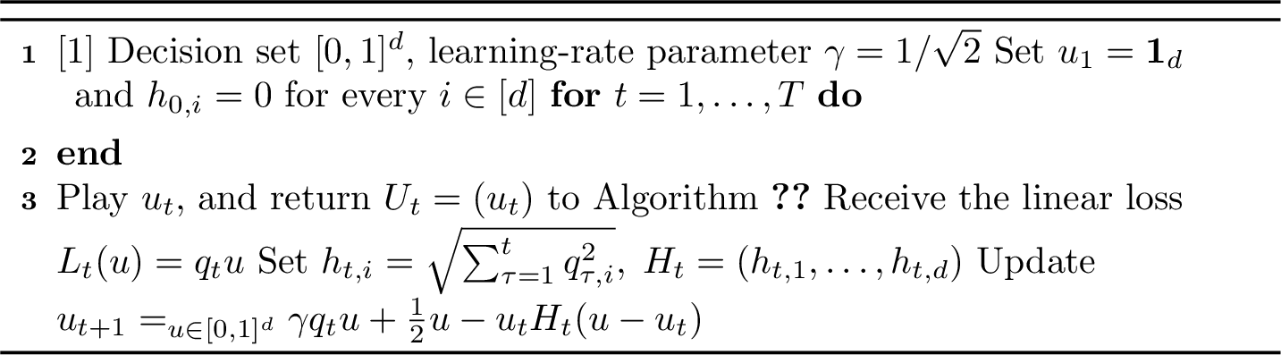
Algorithm 3 is the composite mirror-descent form of diagonal AdaGrad. Coordinatewise, its update is \(u_{t+1,i} = \Pi_{[0,1]} \left( u_{t,i} - \frac{\gamma q_{t,i}}{h_{t,i}} \right)\) ,where the ratio is defined to be zero whenever \(h_{t,i}=0\). We use this algorithm as the online convex optimization algorithm \(\cA\) in Algorithm 1.

Theorem 5 and Corollary 6 of [59] establish the fixed-comparator static-regret guarantee for this update. Since the \(\ell_\infty\)-distance between any \(u\in[0,1]^d\) and the identity comparator \(\mathbf{1}_d\) is at most one, setting \(\gamma=1/\sqrt{2}\) gives, for every realized loss sequence, \[\begin{align} \text{Reg}_T(\cA_{\rm Ada},I_d) &:= \sum_{t=1}^T \left[ L_t(\diag(u_t))-L_t(I_d) \right] = \sum_{t=1}^T \inner{q_t}{u_t-\mathbf{1}_d} \le \sqrt{2} \sum_{i=1}^d \sqrt{ \sum_{t=1}^T q_{t,i}^2 }. \end{align}\] This inequality is pathwise and therefore remains valid when the linear losses are generated adaptively. Taking expectations yields \(\mathscr R_T(\cA_{\rm Ada},I_d) \le \sqrt{2}\, \EE\left[ \sum_{i=1}^d \sqrt{ \sum_{t=1}^T q_{t,i}^2 } \right].\)

The preceding bound has a direct expression in terms of the stochastic gradients used by our reduction. Since \(\|m_t\|_2\le G_0=\sqrt{2}G\), we have \(|q_{t,i}| = \frac{|s_{t,i}m_{t,i}|}{G} \le \sqrt{2}|s_{t,i}|.\) Consequently, \[\mathscr R_T(\cA_{\rm Ada},I_d) \le 2\, \EE\left[ \sum_{i=1}^d \sqrt{ \sum_{t=1}^T s_{t,i}^2 } \right].\] Substituting this data-dependent regret bound into Theorem 1 gives \[\begin{align} \frac{1}{T}\sum_{t=1}^T \EE\left[\|\nabla f(x_t)\|_2^2\right] \lesssim & \frac{\sigma G}{\sqrt T} + \frac{G}{T} \EE\left[ \sum_{i=1}^d \sqrt{ \sum_{t=1}^T s_{t,i}^2 } \right] + \frac{G^2}{T}. \end{align}\]

This expression preserves the coordinatewise geometry of AdaGrad. For comparison, Euclidean OGD on the same decision set \([0,1]^d\) produces a regret term proportional to \(\sqrt d \sqrt{ \sum_{i=1}^d\sum_{t=1}^T q_{t,i}^2 },\) whereas diagonal AdaGrad produces \(\sum_{i=1}^d \sqrt{ \sum_{t=1}^T q_{t,i}^2 }.\) The AdaGrad term is never larger up to universal constants and can be smaller by a factor of order \(\sqrt d\), for example when the observed OCO-gradient energy is concentrated in a single coordinate [59].

We can also obtain an instance-independent regret bound using only the assumptions of Theorem 1. Smoothness and the range bound imply \(\|\nabla f(x)\|_2^2\le 2M\beta.\) Therefore, we have \[\begin{align} \EE[\|s_t\|_2^2] &= \EE[\|\nabla f(x_t)\|_2^2] + \EE[\|s_t-\nabla f(x_t)\|_2^2]\le 2M\beta+\sigma^2. \end{align}\] By Jensen’s and Cauchy–Schwarz inequalities, \[\begin{align} \EE\left[ \sum_{i=1}^d \sqrt{ \sum_{t=1}^T s_{t,i}^2 } \right] \le \sum_{i=1}^d \sqrt{ \sum_{t=1}^T\EE[s_{t,i}^2] } \le \sqrt{ d\sum_{t=1}^T\EE[\|s_t\|_2^2] } \le \sqrt{ dT(2M\beta+\sigma^2) }. \end{align}\] We obtain \(\mathscr R_T(\cA_{\rm Ada},I_d) \le 2\sqrt{ dT(2M\beta+\sigma^2) }.\) Plugging this bound into Theorem 1 yields \[\begin{align} \frac{1}{T}\sum_{t=1}^T \EE\left[\|\nabla f(x_t)\|_2^2\right] \lesssim& \frac{\sigma\sqrt{M\beta}}{\sqrt T} + \frac{ \sqrt{ dM\beta(2M\beta+\sigma^2) } }{\sqrt T} + \frac{M\beta}{T}. \end{align}\] Thus, the diagonal AdaGrad oracle preserves the \(O(T^{-1/2})\) smooth nonconvex convergence rate while retaining a sharper instance-dependent coordinatewise guarantee.

8.2 Preconditioner Selection via Shampoo↩︎

Shampoo is an optimizer that extends adaptive diagonal scaling to structured matrix and tensor parameters [14]. For a matrix parameter \(W_t\in\RR^{p\times q}\), Shampoo accumulates second-moment information separately along the row and column modes. The corresponding left and right preconditioners retain correlations within each mode without constructing a full \(pq\times pq\) preconditioning matrix.

For our reduction, we apply the same matrix-adaptive online geometry to the preconditioner decision rather than directly to the model parameter.

Consider the set \(\cU_{\text{mat}} := \cbr{ U\in\cS^{d\times d}: 0\preceq U\preceq I_d }\). This set is compact and convex, contains \(I_d\), and satisfies the conditions imposed on \(\cU\) in Algorithm 1. For matrices, define the Frobenius inner product by \(\inner{A}{B}_{\mathrm F} := \operatorname{Tr}(A^\top B)\). Since every \(U\in\cU_{\rm mat}\) is symmetric, the loss in Algorithm 1 admits the representation \[\begin{align} L_t(U) = \inner{Q_t}{U}_{\mathrm F},\; Q_t := -\frac{1}{2G} \left( s_tm_t^\top+m_ts_t^\top \right), \end{align}\] where \(s_t\) and \(m_t\) are gathered from Algorithm 1. Indeed, we have \[\begin{align} \inner{Q_t}{U}_{\mathrm F} &= -\frac{1}{2G} \operatorname{Tr} \left[ \left( m_ts_t^\top+s_tm_t^\top \right)U \right] = -\frac{1}{G}s_t^\top U m_t = L_t(U). \end{align}\] The symmetrization is necessary because the OCO decision space consists of symmetric matrices. Moreover, we have \(\rank(Q_t)\le 2\), which is precisely the low-rank structural condition appearing in the Shampoo regret theorem [14].

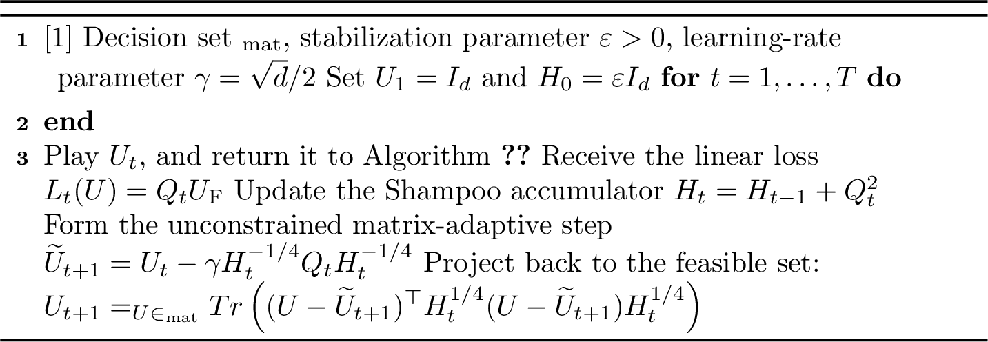
The projection in Algorithm 4 is part of the theoretical OCO oracle. It guarantees that every play remains feasible and that \(\|U_t-I_d\|_{\mathrm F}\le \sqrt d\). The bounded-domain projected version and its weighted projection are discussed by [14].

Theorem 7 of [14] gives the following fixed-comparator guarantee. If the matrix gradients have rank at most \(r\), then the projected Shampoo update satisfies \[\sum_{t=1}^T \left[ L_t(U_t)-L_t(U) \right] \le \sqrt{2r}D \operatorname{Tr}(H_T^{1/4}) \operatorname{Tr}(H_T^{1/4}),\] where \(D\) is any upper bound on \(\max_t\|U_t-U\|_{\mathrm F}\), and the learning-rate parameter is chosen as \(\gamma=\frac{D}{\sqrt{2r}}.\) For the identity comparator, we may take \(D=\sqrt d\). Since \(\rank(Q_t)\le2\), we set \(r=2\), which gives \(\gamma=\sqrt d/2\). Therefore, for every realized loss sequence, \[\begin{align} \text{Reg}_T(\cA_{\rm Shampoo},I_d) &:= \sum_{t=1}^T \left[ L_t(U_t)-L_t(I_d) \right] \le 2\sqrt d\, \left[ \operatorname{Tr}(H_T^{1/4}) \right]^2. \end{align}\] Taking expectations gives the data-dependent static-regret bound \[\mathscr R_T(\cA_{\rm Shampoo},I_d) \le 2\sqrt d\, \EE\left[ \left[ \operatorname{Tr}(H_T^{1/4}) \right]^2 \right].\] This trace expression retains the spectral structure of the matrix OCO gradients \(Q_1,\ldots,Q_T\). It is therefore the matrix analogue of the coordinatewise data-dependent term in diagonal AdaGrad.

For completeness, we next derive an instance-independent consequence. Let \(\lambda_1,\ldots,\lambda_d\) denote the eigenvalues of \(H_T\). Two applications of Cauchy–Schwarz yield \[\begin{align} \left[ \operatorname{Tr}(H_T^{1/4}) \right]^2 = \left( \sum_{i=1}^d\lambda_i^{1/4} \right)^2 \le d\sum_{i=1}^d\lambda_i^{1/2} \le d^{3/2} \sqrt{ \sum_{i=1}^d\lambda_i } = d^{3/2} \sqrt{\operatorname{Tr}(H_T)}. \end{align}\] Furthermore, by algebra, we have \(\operatorname{Tr}(H_T) = d\varepsilon+ \sum_{t=1}^T\|Q_t\|_{\mathrm F}^2\). Because symmetrization is an orthogonal projection under the Frobenius norm, we have \(\|Q_t\|_{\mathrm F} \le \frac{\|s_tm_t^\top\|_{\mathrm F}}{G} \le \sqrt{2}\|s_t\|_2.\) Consequently, we obtain \(\EE[\|Q_t\|_{\mathrm F}^2] \le 2\EE[\|s_t\|_2^2] \le 2(2M\beta+\sigma^2)\). Using Jensen’s inequality, we conclude that \[\begin{align} \mathscr R_T(\cA_{\rm Shampoo},I_d) \le 2d^2 \EE\left[ \sqrt{ d\varepsilon+ \sum_{t=1}^T\|Q_t\|_{\mathrm F}^2 } \right] \le 2d^2 \sqrt{ d\varepsilon+ 2T(2M\beta+\sigma^2) }. \end{align}\] Thus, for fixed \(d\) and \(\varepsilon\), we have \(\mathscr R_T(\cA_{\rm Shampoo},I_d) = O(\sqrt T).\) Substituting the explicit bound into Theorem 1 gives \[\begin{align} \frac{1}{T}\sum_{t=1}^T \EE\left[\|\nabla f(x_t)\|_2^2\right] \lesssim& \frac{\sigma\sqrt{M\beta}}{\sqrt T} + \frac{d^2\sqrt{M\beta}}{T} \sqrt{ d\varepsilon+ 2T(2M\beta+\sigma^2) } + \frac{\beta}{T}. \end{align}\] Therefore, the projected Shampoo oracle also yields an \(O(T^{-1/2})\) convergence guarantee for smooth stochastic nonconvex optimization. The trace-dependent bound is the more informative form, since it can be substantially smaller than the instance-independent bound when the OCO loss matrices possess favorable low-rank or anisotropic spectral structure.

Finally, the same two OCO algorithms can be used as black-box static-regret oracles in the nonsmooth reduction. In that case, only the linear loss gradient supplied by the outer reduction changes; the pathwise static-regret guarantees of diagonal AdaGrad and projected Shampoo remain unchanged.

9 Discussion↩︎

In this paper, we establish, to the best of our knowledge, the first black-box reduction from offline stochastic nonconvex optimization to undiscounted static-regret minimization in online convex optimization. Under the bounded-range assumptions considered here, our results provide an affirmative resolution to the open problem posed by [1]. The key idea is to use a static-regret minimization oracle to adaptively select a preconditioner rather than to determine the optimization iterate or descent direction directly. This separation allows the nonconvex procedure to generate the descent signal while the online learner controls its geometry, making the reduction modular and black-box.

Our framework applies to both smooth and nonsmooth stochastic nonconvex objectives. In the smooth setting, an OCO oracle with \(O(\sqrt{T})\) static regret recovers the classical \(O(T^{-1/2})\) convergence rate. In the nonsmooth setting, the same reduction continues to rely only on ordinary undiscounted static regret and achieves the optimal \(O(T^{-2/7})\) rate for the relaxed distributional stationarity measure considered in this paper. Moreover, the diagonal AdaGrad and projected Shampoo examples illustrate how coordinatewise and matrix-adaptive online-learning geometries can be instantiated as preconditioner-selection oracles. Their data-dependent regret bounds translate directly into data-dependent nonconvex convergence guarantees, providing a unified perspective on adaptive preconditioning.

A natural direction for future research is to determine whether the online-learning mechanisms underlying methods such as Adam [12], Muon [10], and Lion [15] can be reformulated—or suitably modified—to fit the same preconditioner-space static-regret interface. More broadly, our results suggest a modular principle for optimizer design: any compatible OCO algorithm with an appropriate static-regret guarantee can serve as a preconditioner-selection module for stochastic nonconvex optimization. Exploring the limits of this principle, weakening the assumptions required by the reduction, and studying the theoretical and practical properties of the resulting algorithms are important directions for future work.

10 Mathematical Tools↩︎

11 Proofs in Section 6↩︎

In this section, we provide proofs in Section 6. First, we will provide and prove several lemmas that are useful throughout the paper.

Equipped with these lemmas, we are ready to analyze the error of the predictable tracker \(m_t\). From the update \(x_{t+1}-x_t=-\eta U_tm_t\). The key is that \(m_t\) should not be too far from the gradient \(g_t=\nabla f(x_t)\). Specifically, we define the following quantities. \[e_t=m_t-g_t,\;E_{tr}=\sum_{t=1}^{T}\EE[\|e_t\|^2],\;S=\sum_{t=1}^{T}\EE[\|g_t\|^2]=\sum_{t=1}^{T}\EE[\|\nabla f(x_t)\|^2],\;V_T=\sum_{t=1}^{T}\EE[\|s_t-g_t\|^2].\] Regarding these quantities, we have the following important lemma.

Now, we provide the following lemma, which says that the total loss obtained through our Algorithm 1 has a descent lower bound.

Equipped with these lemmas, we are finally ready to prove our main theoretical guarantee.

12 Proofs in Section 7↩︎

Throughout this subsection, we write \[b:=1-a, \; g_t:=\nabla f(y_t), \; \xi_t:=s_t-g_t,\] and use the following notations: \[c_t=1-b^t, \; q_{t,s}=\frac{ab^{t-s}}{c_t}, \quad 1\le s\le t.\] Moreover, we use \(\cH_t^-\) to denote the \(\sigma\) algebra generated by the history \(\cbr{x_i,U_i,z_i,m_i}_{i<t}\cup\cbr{x_t,U_t,z_t}\) and use \(\cH_t\) to denote the \(\sigma\) algebra generated by \(\cbr{x_i,U_i,z_i,m_i}_{i<t}\cup\cbr{U_t,z_t,r_t}\). Therefore, by our update rule, we know that \(x_t,m_t,z_t,U_t,\delta_t,x_{t+1}\) are \(\cH_t^-\) measurable, and \(y_t,g_t\) is \(\cH_t\) measurable.

By the conditional stochastic-oracle Assumption 2, we have \[\EE[s_t\mid \cH_t]=g_t, \; \EE[\|s_t-g_t\|_2^2\mid \cH_t]\le\sigma^2,\] as well as the conditions regarding the preconditioner decision set \[I_d\in\cU, \; \|U\|_{\mathrm{op}}\le1 \quad\text{for every }U\in\cU.\] All expectations below are taken over the randomness of the OCO oracle, the segment variables \(r_t\), the stochastic-gradient oracle, and the output index \(\tau\).

Recall also the local stationarity measure \[\label{eq:detailed95ns95stationarity95definition} \|\nabla f(x)\|^{[\lambda]} := \inf_{\substack{p\in\mathcal{P}(\RR^d)\\ \EE_{X\sim p}[X]=x}} \left\{ \left\|\EE_{X\sim p}[\nabla f(X)]\right\|_2 + \lambda\EE_{X\sim p}\|X-x\|_2^2 \right\}.\tag{4}\]

The proof is organized through a sequence of auxiliary lemmas. We first replace the unavailable smooth descent lemma with an exact random-segment identity. Static regret against the identity matrix then controls the predictable tracker. We subsequently relate that stochastic tracker to a weighted average of true gradients, bound the spatial dispersion of the associated query points, and combine the two estimates into a local stationarity certificate.

The first lemma explains the role of the random segment query. Averaging the directional derivative over the segment from \(x_t\) to \(x_{t+1}\) recovers the exact function difference, even though no Lipschitz-continuous gradient is available.

The preceding lemma controls the cumulative loss of the matrices actually played by the OCO oracle. The next lemma transfers this control to the fixed identity comparator. It is the unique point at which the black-box static regret guarantee enters the nonsmooth analysis.

The identity-comparator loss is a correlation between the stochastic gradient and the normalized predictable direction. The next lemma converts this cumulative correlation into a bound on the average magnitude of the tracker. Its proof introduces the smoothed norm \(\Phi_\rho(m)=\sqrt{\|m\|_2^2+\rho^2}\) and shows explicitly that the contraction by \(b=1-a\) creates a potential leakage proportional to \(\|m_t\|_2\).

The tracker \(m_t\) is formed from stochastic samples, whereas the stationarity measure is defined using true gradients. We therefore introduce a proof-only tracker \(h_t\) driven by \(g_t=\nabla f(y_t)\). The next lemma uses projection nonexpansiveness and conditional unbiasedness to control \(m_t-h_t\), without invoking any continuity property of the gradient.

The geometric output weights are chosen to coincide exactly with the coefficients obtained by unrolling the true-gradient tracker. The following lemma combines that algebraic identity with the distribution of \(\tau\). This converts the mean gradient of the output witness into an unweighted average of tracker norms, plus the stochastic tracking error and one terminal normalization term.

Since \(h_{t+1}=a\sum_{s=1}^{t}b^{t-s}g_s\), we define the re-normalized coefficients as \[c_t:=a\sum_{s=1}^tb^{t-s}=1-b^t, q_{t,s}:=\frac{ab^{t-s}}{c_t},\] then \(\sum_{s=1}^{t}q_{t,s}=1\) and \(\cbr{q_{t,s}}_{s=1}^t\) form a discrete distribution.

By some algebra, if we sample according to \(\PP(Y=y_s)=q_{t,s}\), then we have \(\EE[Y]=\sum_{s=1}^tq_{t,s}y_s=\bar y_t\) and \(\EE[\nabla f(Y)]=\sum_{s=1}^tq_{t,s}g_s=\frac{h_{t+1}}{c_t}\).

The averaged-gradient estimate alone does not yet yield local stationarity: the witness distribution must also be concentrated around its mean. The next lemma controls this spatial variance. Its proof separates the displacement inside each randomly queried segment from the accumulated motion of the base iterates, and then computes the coefficient of every individual increment \(\delta_k\).

We now possess the two components required by the definition of local stationarity. Lemma 12 controls the mean gradient of a discrete witness distribution, while Lemma 13 controls the second moment of that distribution around its mean. The following lemma combines these components, but deliberately leaves the average tracker norm unsubstituted so that the final theorem proof has a transparent modular form.

With all the lemmas above, we are now ready to assemble them to prove Theorem 2; no additional probabilistic or optimization argument is needed beyond the lemmas above.

References↩︎

---

1. Email: huhc@mit.edu↩︎

2. Email: dslevi@mit.edu↩︎