Panache: One-Pass Motif Discovery at Every Window Length
July 20, 2026
Abstract
Motif discovery, the search for recurring patterns within a time series, is a core primitive of exploratory data analysis. A pattern, however, is defined by its duration, which analysts rarely know in advance. To resolve this unknown duration, an interval of window lengths is defined, and the accepted method is to try every length in that interval. Existing pan matrix profile (PMP) methods compute one z-normalized matrix profile per length, so \(L\) lengths cost \(L\) quadratic self-joins over the same series. We introduce Panache, to our knowledge the first one-pass streaming algorithm for z-normalized PMP motif discovery. It replaces the repeated self-joins with a single scan whose runtime is near-linear in the series length. The key observation is that mean-centering a subsequence changes only its DC Fourier coefficient, so the non-DC spectrum of every z-normalized subsequence can be maintained online by sliding-DFT recurrences and running statistics. This spectral state is the key under which similar subsequences collide in an occupancy-controlled hash directory and, through Parseval’s theorem, yields a lower bound that rejects most colliding pairs before any exact computation. Panache computes every data-dependent parameter itself, leaving only a resource budget to tune. At the default budget, it recovers all top-20 pan-motifs against exact fixed-exclusion ground truth on 17 UCR configurations, and is faster than every CPU and GPU baseline benchmarked in this paper. On Wafer at five million samples over 51 lengths, Panache completes one pass in 2.9 minutes and emits the exact motifs in 6.0 minutes, against 7.95 hours for the fastest exact CPU baseline and 38.3 minutes for Scamp on an H100 GPU.
<ccs2012> <concept> <concept_id>10002951.10003227.10003351</concept_id> <concept_desc>Information systems Data mining</concept_desc> <concept_significance>500</concept_significance> </concept> <concept> <concept_id>10003752.10003809.10010047</concept_id> <concept_desc>Theory of computation Streaming, sublinear and near linear time algorithms</concept_desc> <concept_significance>300</concept_significance> </concept> </ccs2012>
1 Introduction↩︎
Time-series motif discovery looks for subsequences that recur in the same series [1], [2]. The difficulty is that a motif is not defined until a duration is chosen. A window length \(m\) represents a duration. It determines which subsequences are compared and what it means for two occurrences to have the same shape. Too short a window fragments the event; too long a window mixes the event with its context. In exploratory data analysis, this duration is often the unknown rather than an input the analyst can set reliably.
The matrix profile [3] replaced the varying definitions of a motif with a single formulation. For a chosen window length \(m\), a fixed-length algorithm starts by initializing a window and computing its z-normalized distance to all valid non-overlapping windows of the same length in the entire series (Figure 1). The window that achieved the smallest of these distances is the nearest neighbor. When the same window advances by one position, distances are recomputed across the entire series again. This process is repeated from the start of the series to the end, producing a quadratic self-join, and one self-join yields one row, the matrix profile \(P_m\), which stores each window’s nearest-neighbor distance. Each stored entry is a cell, and motifs are the cells of \(P_m\) with the smallest distances rather than the outcome of a separate combinatorial search. The speed of these algorithms comes from recurrences that reuse dot products while two windows of the same length slide together. The reuse makes each evaluation cheap, but it never makes evaluations fewer. This formulation is why fixed-length motif discovery has mature exact algorithms [4]–[7].
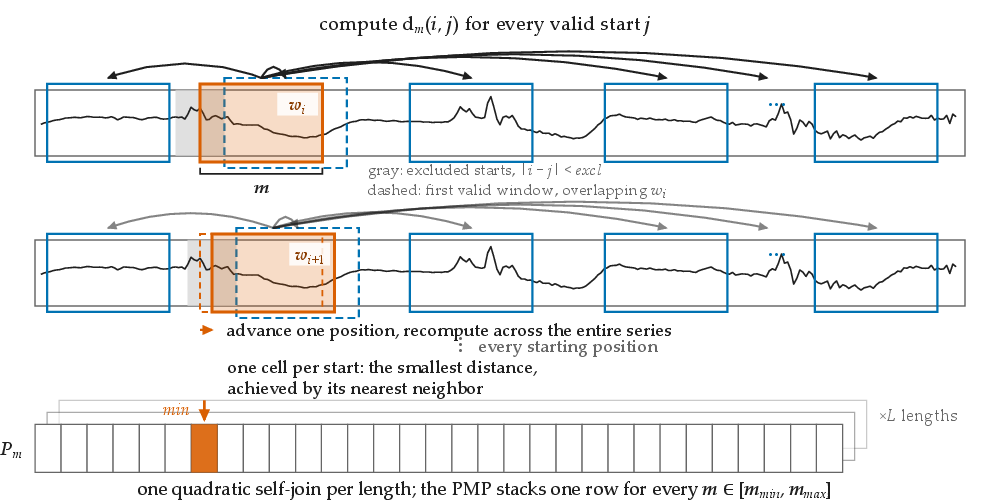
The pan matrix profile (PMP) [8] replaces the duration choice with an interval of lengths. It computes a matrix profile for every length and stacks each profile for every \(m\in[m_{\min},m_{\max}]\). Existing PMP algorithms achieve this generality through repetition. The computations performed at one length are never reused at another, because every length changes the set of windows, the overlap rule that rejects trivial matches, the mean and standard deviation that z-normalize every window, and the length-\(m\) Fourier basis used by the FFT steps. The recurrences never cross lengths either. Every single window length forces its own rescan of the entire series, and that just by taking one slide. The cost increases with every length in the interval.
We present Panache, to our knowledge the first one-pass streaming algorithm for z-normalized PMP motif discovery. Panache scans the series once while maintaining a single multi-length search state. Each sample is consumed on arrival and advances the whole multi-length state at once. No length and no slide ever forces a rescan of the series. From this state it selects which subsequence pairs to evaluate. A profile cell is updated only with the exact z-normalized distance of a valid pair (§2). Every written cell therefore holds an exact distance to a valid neighbor.
The central representation is the normalized AC spectrum of a window. If \(X_k\) is a Fourier coefficient of a window, subtracting the window mean changes only \(X_0\). Every coefficient with \(k>0\) is unchanged by centering and is divided only by the window standard deviation. The non-DC coefficients can therefore be maintained online by sliding-DFT recurrences. Beyond serving as the streaming state, this vector is the SimHash key [9], a locality-sensitive hash (LSH) under which windows of similar normalized shape collide. The same vector gives the Parseval lower bound that rejects most candidate pairs before exact distance computation.
We introduce four mechanisms that make this representation scale with a growing stream. Anchor lengths restrict the online state to a subset of the interval’s lengths, relying on the persistence of motifs across neighboring lengths. Similar windows collide in the same hash bucket, and occupancy-controlled prefix hashing keeps mean bucket occupancy near a fixed target as the series grows, so a constant per-query budget stays effective for all but the densest classes. Exclusion-zone batching parallelizes the stream while leaving the output bit-identical to serial processing at any thread count. A final emit stage materializes the profile with exact comparisons inside oversized buckets and around the discovered motifs.
Our contributions are as follows.
A formulation of one-pass PMP motif discovery around a sound upper pan-profile, which guarantees exact distances and valid neighbors for every written cell (§2).
A normalized AC-spectrum representation whose non-DC coefficients are maintained online and serve simultaneously as the streaming state, the SimHash key, and a Parseval rejection bound (§3.2).
The mechanisms required at scale: occupancy-controlled global-depth hashing, anchor-length search, deterministic exclusion-zone batching, and emit-time completion (§3.3–3.6).
An evaluation on ten UCR datasets across 17 exact-ground-truth configurations, with full top-20 recovery, faster runtime than every comparable public CPU and GPU baseline, and per-configuration statistics of the recovered motif values (§4). Every data-dependent parameter is computed by the algorithm itself, and every design constant stayed at its default in every experiment.
2 Background and Problem↩︎
A time series is a vector \(T=(t_0,\ldots,t_{n-1})\). For a window length \(m\), write \(T_{i,m}=(t_i,\ldots,t_{i+m-1})\), with \(0\le i<n-m+1\), for the subsequence starting at position \(i\). Its z-normalized form is \(Z_{i,m}=(T_{i,m}-\mu_{i,m}\mathbf{1})/\sigma_{i,m}\), where constant windows, for which \(\sigma_{i,m}=0\), are ignored. The distance between two subsequences of length \(m\) is the Euclidean distance after z-normalization, \(\mathrm{d}_m(i,j)=\lVert Z_{i,m}-Z_{j,m}\rVert_2\), equivalently \(\mathrm{d}_m(i,j)^2 = 2m(1-\rho_m(i,j))\) for their Pearson correlation \(\rho_m(i,j)\). Exact matrix-profile algorithms exploit this identity. The correlation is the raw dot product corrected by the window moments, \(m\,\rho_m(i,j)=(T_{i,m}\cdot T_{j,m}-m\,\mu_{i,m}\mu_{j,m}) /(\sigma_{i,m}\sigma_{j,m})\). One dot product and the moments \(\mu,\sigma\) of both windows therefore determine the distance in closed form, without re-reading the samples [3], [6]. In this paper, an exact distance is the value \(\mathrm{d}_m(i,j)\) itself, never an estimate or a bound.
In a self-join, windows whose starts are very close share most of their samples and are not considered motif pairs. A pair is valid when its start positions satisfy \(|i-j|\ge \mathit{excl}\), for a fixed exclusion parameter \(\mathit{excl}\) [1], [10]. For one length \(m\), the matrix profile is the row pair \((P_m,I_m)\) [3], \[P_m[i] = \min_{\substack{j\\ |i-j|\ge \mathit{excl}}} \mathrm{d}_m(i,j), \qquad I_m[i] \in \arg\min_{\substack{j\\ |i-j|\ge \mathit{excl}}} \mathrm{d}_m(i,j).\]
The pan matrix profile (PMP) [8] is the stack of these rows over an interval \([m_{\min},m_{\max}]\). Let \(L=m_{\max}-m_{\min}+1\). A pan-motif is a low cell of this stack together with its nearest-neighbor index. To avoid reporting the same region repeatedly, the top-\(k\) list is formed by sorting cells by distance and skipping any cell that lies within \(m/2\) of an already accepted cell at the same length.
2.0.0.1 The streaming target.
The exact PMP contains \(\sum_{m}(n-m+1)\) cells, each requiring a nearest-neighbor search among the windows of its own length. Panache maintains a relaxation of this object. A sound upper pan-profile is a stack of rows \((\hat{P}_m,\hat{I}_m)\) satisfying, for every cell, either \(\hat{P}_m[i]=\infty\) or \[\hat{P}_m[i]=\mathrm{d}_m(i,\hat{I}_m[i]) \quad\text{with}\quad |i-\hat{I}_m[i]|\ge \mathit{excl},\] and in all cases \(\hat{P}_m[i]\ge P_m[i]\). If \(\hat{P}_m[i]<\infty\), then \(\hat{I}_m[i]\) is a valid neighbor and \(\hat{P}_m[i]\) is its exact distance. Only the nearest-neighbor quantifier is relaxed: if the algorithm evaluates the true nearest-neighbor pair, \(\hat{P}_m[i]\) attains the exact profile value \(P_m[i]\); otherwise it remains a valid upper bound, witnessed by an exactly evaluated neighbor. A finite value below the exact profile value cannot occur, because every written value is the exact distance of some valid pair, and the exact value is the minimum over all of them.
2.0.0.2 Problem statement.
The problem tackled in this paper is to process the samples once, in stream order, over the full length interval. The method must maintain a sound upper pan-profile and emit top-\(k\) pan-motifs whose reported distances are exact distances to valid neighbors. It must find, within its single scan, the valid pairs whose exact distances lower the motif cells, without executing the \(L\) self-joins that define the exact PMP. Updates at stream time \(\tau\) may use only \(t_0,\ldots,t_\tau\). Space linear in \(n\) is inherent to the task, since a materialized pan-profile alone has \(\Theta(nL)\) cells. The memory accounting is given in §3.7.
3 The Panache Algorithm↩︎
Every PMP construction, exact or approximate, is characterized by the set of subsequence pairs whose distances it evaluates. Let \(\mathcal{U}=\{(m,i,j):\;m_{\min}\le m\le m_{\max},\; 0\le i<j\le n-m,\;j-i\ge\mathit{excl}\}\) denote the admissible comparison universe. The exact PMP evaluates all of it, which is what the \(L\) self-joins compute. For an evaluated subset \(\mathcal{S}\subseteq\mathcal{U}\), writing \(\langle i,j\rangle=(\min\{i,j\},\max\{i,j\})\), the profile induced by \(\mathcal{S}\) is \[P_m^{\mathcal{S}}[i]=\min_{j:\;(m,\langle i,j\rangle)\in\mathcal{S}} \mathrm{d}_m(i,j),\] with the empty minimum equal to \(\infty\) and \(I_m^{\mathcal{S}}[i]\) a witness of the minimum.
Proposition 1 (Soundness). For every \(\mathcal{S}\subseteq\mathcal{U}\), the induced profile is a sound upper pan-profile: every finite cell equals the exact z-normalized distance to the valid neighbor it stores, and \(P_m^{\mathcal{S}}[i]\ge P_m[i]\) for every cell.
Proof. A finite cell equals \(\mathrm{d}_m(i,j)\) for some evaluated triple \((m,i,j)\in\mathcal{S}\). Every triple of \(\mathcal{U}\) satisfies \(j-i\ge\mathit{excl}\), so the stored neighbor is valid. \(P_m^{\mathcal{S}}[i]\) is a minimum over a subset of the neighbors defining \(P_m[i]\), so it cannot be smaller than \(P_m[i]\). ◻
Panache computes \((\hat{P},\hat{I})=(P^{\mathcal{S}},I^{\mathcal{S}})\) for an evaluated set assembled in one pass, \[\mathcal{S}=\mathcal{S}_{\mathrm{stream}} \cup\mathcal{S}_{\mathrm{hot}} \cup\mathcal{S}_{\mathrm{local}},\] where \(\mathcal{S}_{\mathrm{stream}}\) is generated during the streaming pass (§3.1–3.5) and \(\mathcal{S}_{\mathrm{hot}}\) and \(\mathcal{S}_{\mathrm{local}}\) are added by the emit stage (§3.6). Proposition 1 separates correctness from coverage. Written values are correct for any choice of \(\mathcal{S}\); the remaining design question is which pairs to evaluate.
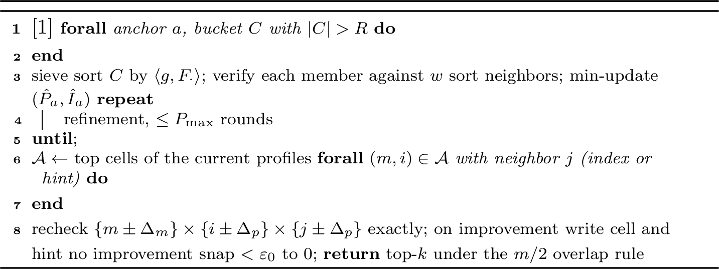
Every such choice must fit within a budget fixed before the stream starts. Per arriving sample and indexed length (§3.3), that budget is \(O(K)\) for the spectral state, \(O(BK)\) for the signature, and at most \(R\) candidate inspections (\(K\): retained spectral width, §3.2; \(B\): signature bits, §3.4; \(R\): verification budget, §3.4). The sections below describe the mechanisms that keep this budget effective as \(n\) grows. Anchor lengths cover the length interval (§3.3), occupancy control keeps the hash directory bounded (§3.4), and exclusion-zone batching parallelizes the stream while keeping the output identical to serial processing (§3.5). Emit-time completion evaluates the oversized hash classes and the motif neighborhoods at non-anchor lengths, completing the evaluated set \(\mathcal{S}\) (§3.6). Algorithms 4 and 5 (appendix) list the update and emit procedures. Figure 2 illustrates each stage on an ECG5000 motif pair (\(i=3925\), \(j=7564\), \(m=20\)), and its panels are referenced throughout the section.
3.1 Windows on a Stream↩︎
An offline PMP computation holds the full series, so a window is identified by where it starts. The algorithm picks a start position and reads the \(m\) samples to its right. A stream allows no such choice. Samples arrive one at a time, and a window can be used only once its last sample has arrived, so the latest published sample decides which windows exist. Windows on a stream are therefore indexed by their right endpoints. Let \(\tau\) be the index of the most recently published sample. A length-\(m\) window with start \(q\) completes at \(\tau=q+m-1\), the moment its last sample arrives. Until then its mean, its variance, its non-DC spectrum, and its distance to any other window do not exist. When sample \(\tau\) is published, exactly one new window completes at every length \(m\le\tau+1\), namely \(T_{\tau-m+1,m}\).
For each anchor length \(a\in A\subseteq[m_{\min},m_{\max}]\), the subset chosen in §3.3, Panache maintains one sliding window. The length-\(a\) window completes for the first time at \(\tau=a-1\), and every later sample slides it to the start \(q=\tau-a+1\) (Figure 2A). Recomputing the window at every slide would read all \(a\) samples for a one-position change. Instead, Panache maintains an online running state (§3.2). At each slide the oldest sample leaves on the left and the newest enters on the right, the state is corrected for exactly those two samples at cost \(O(K)\), and the same state is carried through the entire series. The raw samples are retained, so the exact distance of any pair of completed windows can be computed at any later time.
A sample does not belong to one length. Take lengths 2 and 3 on a stream \(t_0,t_1,t_2,\ldots\). When \(t_1\) arrives, the first length-2 window \((t_0,t_1)\) completes. When \(t_2\) arrives, that window slides to \((t_1,t_2)\), and the first length-3 window \((t_0,t_1,t_2)\) completes. When \(t_3\) arrives, both windows slide at once, to \((t_2,t_3)\) and \((t_1,t_2,t_3)\). The arriving sample \(t_3\) enters both windows, while each window drops a different sample. Every later arrival behaves the same way. Panache holds one running state per anchor length, each published sample advances all of them together, at \(O(K)\) per length and \(O(|A|K)\) in total.
3.2 Normalized Spectral Features↩︎
Each sliding window’s state has three jobs. It must be updated at every slide, provide the signature under which similar windows collide, and yield the Parseval bound that rejects colliding pairs. The normalized non-DC Fourier coefficients do all three.
For a window \(T_{i,m}\), define the DFT coefficients \[X_{i,m,k}=\sum_{r=0}^{m-1}t_{i+r}e^{-2\pi\mathrm{i} kr/m}.\] The coefficient \(X_{i,m,0}\) is proportional to the window mean; the coefficients with \(k>0\) describe variation around that mean level. At an indexed length, Panache retains the scaled prefix \(F_{i,m}=(X_{i,m,1},\ldots,X_{i,m,K'})/\sigma_{i,m}\), zero-padded to the shared width \(K-1\), where \[K'=\min\!\bigl(K-1,\;\lceil m/2\rceil-1\bigr)\] is the number of independent non-DC coefficients at length \(m\): by conjugate symmetry bin \(k\) and bin \(m-k\) are mirror images, and for \(k\ge m\) the index aliases back onto the mean, so only bins \(1\le k\le K'\) carry new shape information (for even \(m\) the Nyquist bin \(m/2\) is omitted). Real and imaginary parts are kept; the DC coefficient is not stored.
Lemma 1 (AC invariance). Let \(\hat{X}_{i,m,k}\) be the DFT coefficient of the z-normalized window \(Z_{i,m}\). For every \(1\le k\le m-1\), \(\hat{X}_{i,m,k}=X_{i,m,k}/\sigma_{i,m}\).
Proof. Centering subtracts \(\mu_{i,m}G_{k,m}\) from coefficient \(k\), where \(G_{k,m}=\sum_{r=0}^{m-1}e^{-2\pi\mathrm{i} kr/m}\). This geometric sum is zero for \(k\not\equiv 0\pmod m\). Scaling by \(\sigma_{i,m}^{-1}\) scales the remaining coefficients. ◻
The stored vector \(F_{i,m}\) therefore equals the leading \(K'\) independent bins of the non-DC spectrum of the z-normalized window (Figure 2A), the remaining entries zero. Mean subtraction affects only the DC bin, and the division by the standard deviation scales all bins uniformly.
3.2.0.1 Online update.
A slide changes the window only at its ends. The departing sample leaves, the arriving sample enters, and every retained sample keeps its value while its position inside the window drops by one. This is the fact the sliding DFT exploits. A DFT coefficient is a sum of samples, each weighted by a phase factor \(e^{-2\pi\mathrm{i}kr/m}\) that depends on its position \(r\). When every position drops by one, every phase factor is multiplied by the same fixed rotation \(e^{2\pi\mathrm{i}k/m}\). One multiplication of the coefficient therefore re-phases all retained samples at once, and nothing is recomputed for them. The only new value entering the sum is the arriving sample.
Formally, let \(S=\sum_r t_{i+r}\) and \(Q=\sum_r t_{i+r}^2\) be the running sum and sum of squares of the current window, with moments \(\mu_{i,m}=S/m\) and \(\sigma_{i,m}^2=Q/m-\mu_{i,m}^2\). When the window advances by one sample, \[\begin{align} S' &= S-t_i+t_{i+m},\qquad Q' = Q-t_i^2+t_{i+m}^2,\\ X_{i+1,m,k} &= e^{2\pi\mathrm{i} k/m}\bigl(X_{i,m,k}-t_i+t_{i+m}\bigr),\\ F_{i+1,m} &= (X_{i+1,m,1},\ldots,X_{i+1,m,K'},0,\ldots,0)/\sigma_{i+1,m}, \end{align}\] so advancing one indexed length by one sample costs \(O(K)\). The update runs in four steps. (i) The running sums advance to \(S'\) and \(Q'\), giving the new moments. (ii) The remove–insert correction \((X_{i,m,k}-t_i+t_{i+m})\) subtracts the departing sample and adds the arriving one to each retained coefficient. (iii) One rotation by the fixed factor \(e^{2\pi\mathrm{i}k/m}\) re-phases all retained samples, as above. Steps ii–iii are the sliding DFT [11], [12]. (iv) The rotated coefficients are divided by the new \(\sigma_{i+1,m}\) to form \(F_{i+1,m}\). Incremental updates accumulate floating-point rounding error, so the implementation recomputes the moments and coefficients from the raw samples every 4,096 slides per anchor.
3.2.0.2 Hash key.
\(F_{i,m}\) is the state that is hashed to a signature and committed to a bucket of a hash directory after every slide. Windows with similar normalized shapes subtend small angles in this truncated spectral space (Figure 2B), and SimHash converts small angles into high collision probability, so similar windows tend to share buckets (the mechanics are the subject of §3.4).
3.2.0.3 Rejection bound.
A collision only proposes a candidate pair. The bound that filters these pairs before any exact computation is built from the same stored vector \(F_{i,m}\). With \(K'\) as defined above, the rejection bound is \[\underline{\mathrm{d}}_{K,m}^2(i,j) =\frac{2}{m}\sum_{k=1}^{K'}|F_{i,m,k}-F_{j,m,k}|^2 .\]
Lemma 2 (Parseval lower bound). For equal-length windows \(i,j\): \(\underline{\mathrm{d}}_{K,m}(i,j)\le \mathrm{d}_m(i,j)\).
By Parseval’s theorem, the squared z-normalized distance equals \(\frac{1}{m}\sum_{k}|\hat{X}_{i,m,k}-\hat{X}_{j,m,k}|^2\) over all \(m\) bins, and the DC term vanishes after z-normalization. Any subset of the remaining terms is a lower bound on the sum. The factor \(2\) accounts for conjugate-symmetric bin pairs of real signals, and the cap on \(K'\) prevents a bin and its alias from being counted twice when \(m<2K\) (proof in Appendix 9). A candidate pair \((i,j)\) is evaluated exactly only if \(\underline{\mathrm{d}}_{K,m}(i,j)\) is smaller than \(\hat{P}_m[i]\) or \(\hat{P}_m[j]\), the two cells that the pair can lower. Otherwise, the exact distance cannot lower either cell, and the pair is skipped. On the ECG5000 example of Figure 2C, this test rejects 214 of the 215 candidates in the probed buckets. Features are cached in single precision. The bound is therefore multiplied by \(1-\lambda\) before the comparison, and Lemma 4 shows that \(\lambda=10^{-4}\) preserves validity at every magnitude where the bound can prune.
3.2.0.4 Spectral width selection.
The spectral width \(K\) sets how many leading Fourier coefficients the state retains. The prefix \(F_{i,m}\) above holds bins \(1\) through \(K'(m)\), zero-padded to the shared width \(K-1\), and the signature and the bound are both built from it, so their precision depends on \(K\). Signatures are compared bit for bit, so every window in the directory must be hashed at one shared width, and \(K\) cannot change once insertion has begun. The width is therefore fixed before insertion begins by a calibration. The calibration step reads sampled windows at each of \(m_{\min}\), the midpoint length, and \(m_{\max}\), in the implementation at most 256 windows for each length, and selects the smallest \(K\) satisfying \[\mathbb{E}\!\left[ \frac{2}{m^2}\sum_{k=1}^{K'}|\hat{X}_{i,m,k}|^2 \right]\ge \eta \quad\text{and}\quad n\,\mathbb{E}\!\left[(1-\theta_K/\pi)^B\right]\le 2\gamma\alpha ,\] where \(\theta_K\) is the sampled angle between \(K\)-dimensional features and \(R=\gamma\alpha\) is the verification budget of §3.4. The first condition requires the retained coefficients to capture a fraction \(\eta\) of the normalized spectral energy, so that features separate windows. A z-normalized window carries total spectral energy \(\sum_k|\hat{X}_{i,m,k}|^2=m^2\), so the criterion leaves, in expectation over the sampled windows, at most \((1-\eta)m^2\) outside the retained bins. Since \(|a-b|^2\le 2|a|^2+2|b|^2\), the expected squared-distance mass invisible to \(\underline{\mathrm{d}}\) is at most \(4(1-\eta)m\), a correlation slack of \(2(1-\eta)\). Larger \(\eta\) therefore tightens pruning at the cost of a larger \(K\). Retaining most of the spectral energy in a small prefix of coefficients is the established practice of the Fourier-indexing tradition [13]–[15], so we set \(\eta=0.85\). The second condition bounds the expected number of accidental signature collisions at the target stream length \(n\) by twice the verification budget. Near-duplicate pairs are excluded from the estimate, since collisions between near-duplicates are the intended behavior. Classes that exceed the budget are handled by the emit stage (§3.6). It is important to notice that the calibration keeps no state and returns only the integer \(K\), so any sample of windows serves, including the earliest windows of a live stream. The pass itself is unchanged. Every sample is read once, in stream order. No choice of \(K\) can invalidate a reported motif. The width decides the cost of the search, never the validity of its output, and recovery is measured unchanged at every admissible width (Appendix 11).
Proposition 2 (Soundness is width-independent). For every width \(K\ge 2\): (i) the bound stays valid, \(\underline{\mathrm{d}}_{K,m}(i,j)\le\mathrm{d}_m(i,j)\) for every equal-length pair, and is non-decreasing in \(K\); (ii) the profile computed at width \(K\) is a sound upper pan-profile (the proof is in Appendix 9).
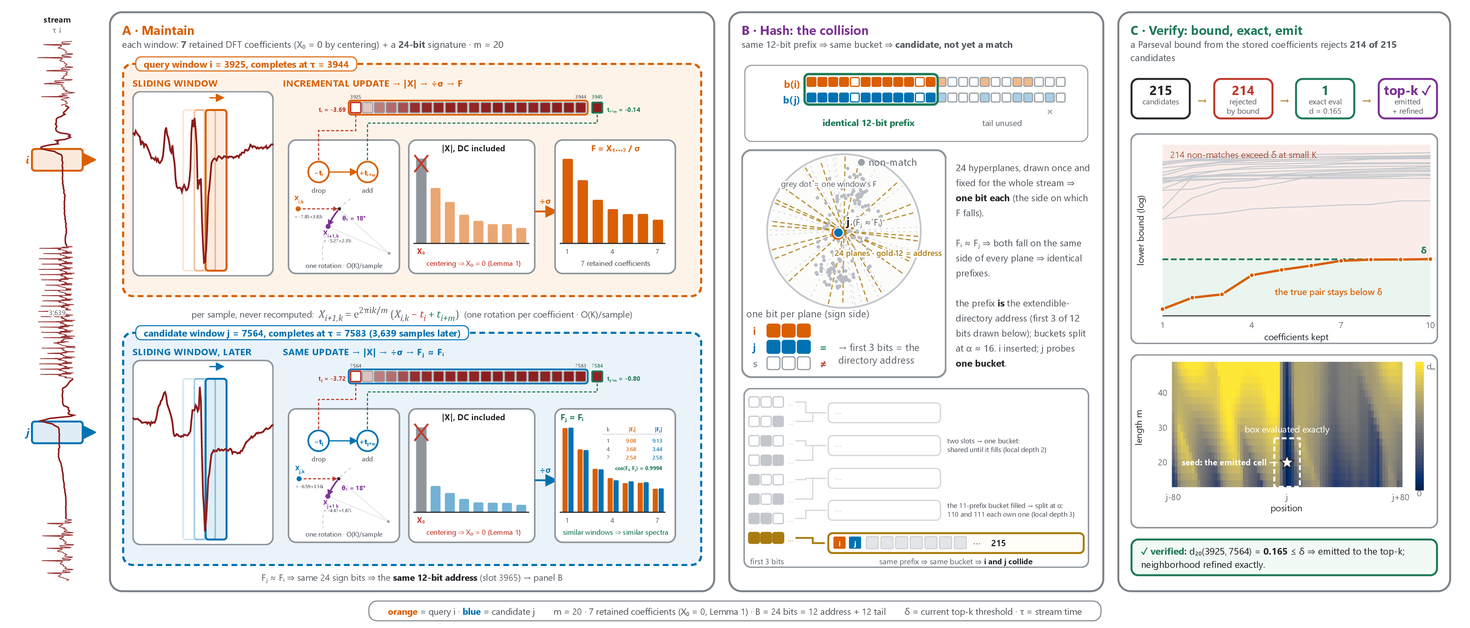
Figure 2: Panache end to end on an ECG5000 motif pair (\(i=3925\), \(j=7564\), \(m=20\)). All values are computed from the data, and the left spine is the stream itself. (A) Each sample updates the retained coefficients in \(O(K)\): drop \(t_i\), add \(t_{i+m}\), one fixed rotation (worked example in each lane); a completed window is normalized to \(F\) and hashed into a 12-bit directory address (§3.1–3.4). (B) \(F_j\approx F_i\): same prefix, same bucket. (C) The Parseval bound rejects 214 of 215 candidates (Lemma 2); the one exact evaluation (\(\mathrm{d}=0.165\)) is emitted and its neighborhood refined (§3.6)..
3.3 Anchor Lengths↩︎
Maintaining an online index at every length in \([m_{\min},m_{\max}]\) would still be one-pass and linear in the stream length, but each arriving sample would pay for \(L\) spectral states, \(L\) directories, and \(L\) probes. Panache optimizes further. It maintains output rows for every length but builds online indexes only at the anchor lengths \(A=\{m_{\min}+rs:\;m_{\min}+rs\le m_{\max}\}\cup\{m_{\max}\}\), for a stride \(s\) and integers \(r\ge 0\), so the online search cost scales with \(|A|=\lceil L/s\rceil\) rather than \(L\). Every experiment in this paper uses \(s=2\) (§[sec:setup]).
The assumption behind anchors is not that motifs occur at anchor durations, but that low PMP cells occupy contiguous regions of the length–position plane. When two subsequences match at length \(m\), their z-normalized distance after re-cutting both one sample longer or shorter is bounded above and below by explicit functions of the distance at length \(m\) [16]. Nearby start positions usually remain in the same low-distance region. A region that spans at least \(s\) consecutive lengths intersects at least one anchor. Each anchor draws its own projection vectors, so the anchors that a region intersects provide multiple, nearly independent opportunities for its discovery (Figure 3).
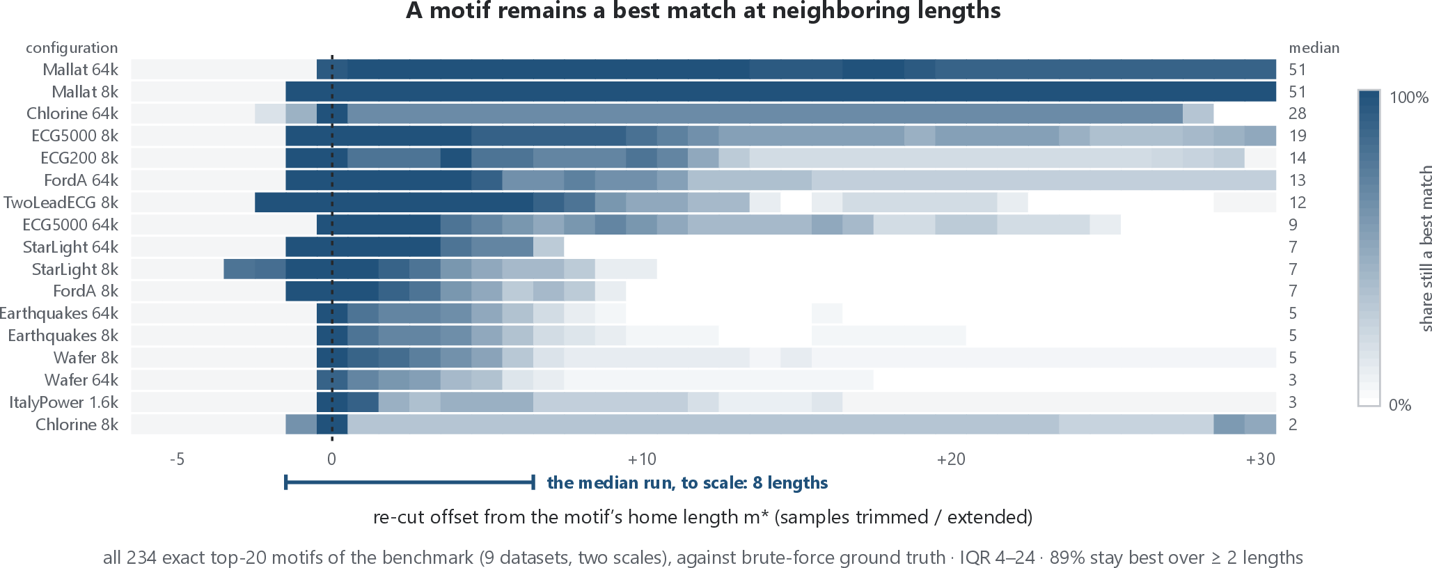
Proposition 3 (Cross-length redundancy). Call a pair matchable at anchor \(a\) if it is valid and would lower at least one profile cell at length \(a\), and let \(M_A\) be the set of anchors at which it is matchable. Let \(p_a\) be the probability that signatures and probes collide at anchor \(a\), and \(c_a\) the probability that the budgeted scan retains the pair after collision. Since the per-anchor projections are drawn independently (§3.4), the probability that no anchor discovers the pair is at most \(\prod_{a\in M_A}(1-p_ac_a)\) (proof in Appendix 9).
The proposition quantifies the redundancy that anchors provide. The probabilities \(p_a\) and \(c_a\) are data dependent, so recall is evaluated empirically (§4), while soundness (Prop. 1) and determinism (Prop. 5) hold unconditionally. Anchoring skips lengths on purpose, and the skipped lengths carry no online state. They are still searched. Every motif emitted at an anchor length starts a local completion (§3.6), which evaluates exact distances at the neighboring lengths and positions around the emitted pair, and the contiguity of low regions is exactly what makes these neighborhoods the right place to look. A low region that spans fewer than \(s\) consecutive lengths can still escape every anchor. A smaller stride or a wider completion neighborhood moves the method toward dense coverage at higher cost.
3.4 Streaming Candidate Generation↩︎
For every anchor length, an individual hash directory is maintained, so a window is only ever compared against earlier windows of the same length. Earlier start positions are stored under a SimHash signature of their feature vectors. Bit \(\ell\) of the signature of a start \(i\) at anchor \(a\) is \(b_a(i)_\ell=\mathbf{1}\{\langle g_{a,\ell},F_{i,a}\rangle\ge 0\}\) for \(\ell=1,\ldots,B\), where \(g_{a,\ell}\) are seeded Gaussian projections drawn independently per anchor. The per-anchor draw is what makes the anchors’ discovery attempts nearly independent (Prop. 3).
Fact 1 ([9]). For a standard Gaussian projection \(g\) and vectors \(u,v\) at angle \(\theta\), \(\Pr[\mathrm{sign}\langle g,u\rangle\ne \mathrm{sign}\langle g,v\rangle]=\theta/\pi\).
Windows whose normalized shapes are close therefore agree on each signature bit with high probability (Figure 2B). A hash table with a fixed number of buckets, however, degrades as the stream grows. Bucket populations increase linearly with \(n\) while the per-query budget is constant, so either the budget is exceeded or queries compare only against recent arrivals. Panache controls bucket size with a global-depth prefix directory, a variant of extendible hashing [17] in which every bucket shares one directory-wide depth \(d\) rather than carrying a per-bucket local depth. The bucket address of a window is the \(d\)-bit prefix of its signature. When the number of stored windows exceeds \(\alpha 2^{d}\) for an occupancy target \(\alpha\), and unused signature bits remain (\(d<B\)), the entire directory doubles: the depth increases to \(d+1\) and every entry is rehomed by its next signature bit, available because full signatures are stored. No individual bucket splits on its own and no local depths are kept; a single depth \(d\) governs the whole anchor’s directory.
Proposition 4 (Occupancy control). Splitting whenever the population exceeds \(\alpha 2^d\) keeps mean bucket occupancy at most \(\alpha\), and within \((\alpha/2,\alpha]\) between splits after the initial fill; the total rehoming work amortizes to \(O(1)\) per insertion until the signature or implementation depth limit is reached (proof in Appendix 9).
Deeper prefixes reduce bucket size but also reduce the probability that two similar windows share a full prefix. The query side compensates by multi-probing [18]. A query inspects its exact prefix bucket and then buckets at Hamming distance one, in increasing order of the projection margin \(|\langle g_{a,\ell},F_{q,a}\rangle|\). A small margin indicates a bit that was close to the decision boundary, so the corresponding one-bit variants are the most probable alternative buckets. The number of Hamming-1 probes grows with depth as \(1+\max(0,\,d-d_0)\), for a reference depth \(d_0\), capped by the depth and an implementation limit. Candidates from the probed buckets are deduplicated, filtered by the exclusion rule, and inspected up to the budget \(R=\gamma\alpha\), a fixed multiple \(\gamma\) of the occupancy target \(\alpha\). The target \(\alpha\) is the only parameter exposed to the analyst. When a probed bucket contains more entries than the remaining budget, half of that budget inspects the most recent entries and the other half inspects entries at even intervals across the whole bucket. This avoids bias toward recent arrivals.
Let \(Q_a(q)\) denote the candidates retained for query start \(q\), with \(|Q_a(q)|\le R\). The streaming pass evaluates exactly the pairs \[\mathcal{S}_{\mathrm{stream}} =\{(a,\langle i,q\rangle): i\in Q_a(q), \underline{\mathrm{d}}_{K,a}(i,q)<\max(\hat{P}_a[i],\hat{P}_a[q])\}.\] Each computed distance updates both cells, \(\hat{P}_a[i]\) and \(\hat{P}_a[q]\). A cell and its neighbor index are overwritten whenever the new distance is smaller.
3.5 Batched Online Updates↩︎
Batching lets Panache run on any number of threads without changing its output. A batch is a group of \(\beta\le\mathit{excl}\) consecutive arriving samples processed together. At a fixed length, the windows completed by one batch have consecutive start positions, all closer than \(\mathit{excl}\), so no two of them can form a valid pair. Windows of the same batch therefore never search each other. The batch is published in full before any of its searches begins. The only windows a search sees early are its own batch-mates, every one of them invalid by the exclusion rule, and skipping an invalid candidate costs none of the verification budget.
A batch runs in three phases. Phase A advances the running state of §3.2 for all anchors in parallel and inserts the completed windows into the directories. Each anchor owns its moments, coefficients, and directory, so the threads share nothing. Phase B searches in parallel, one work unit per completed window. Each unit probes its directory (§3.4), rejects candidates with the bound, computes exact distances for the survivors, and stores the cell improvements in a private buffer. Phase C merges the buffers into the profile in a fixed order of anchor and buffer index, so equal distances resolve to the same neighbor on every run. No batch pair is valid, no state is shared, and the merge order is fixed. Nothing in the schedule can therefore change a result, and a window is searched at most \(\beta-1\) samples after it completes.
Proposition 5 (Determinism). For a fixed input stream, configuration, and seed, the profiles and motifs emitted by Panache are identical for every thread count and schedule (proof in Appendix 9).
4.8pt
@l r | r c r rr | rrrrrrr@ & & &
(lr)3-7(l)8-14 Dataset & & & top-20 (pos+val) & & & & & & & & & &
ECG200 & 8k & 0.06 & 20/20 (16+4) & 37 MB & 0.14 & 32 MB & 0.17 & 0.85 & 4.80 (20) & 8.32 (20) & 8.29 & 50.1 & 20.8 (18)
ItalyPowerDemand & 1,600 & 0.01 & 20/20 (20+0) & 37 MB & 0.02 & 37 MB & 0.04 & 0.21 & 0.52 (20) & 0.91 (20) & 0.90 & 4.83 & 8.48 (20)
Wafer & 8k & 0.08 & 20/20 (19+1) & 37 MB & 0.25 & 51 MB & 0.29 & 1.20 & 7.45 (20) & 12.8 (20) & 13.0 & 81.6 & 117 (20)
Earthquakes & 8k & 0.07 & 20/20 (20+0) & 37 MB & 0.25 & 64 MB & 0.30 & 1.16 & 7.13 (20) & 12.8 (20) & 13.0 & 81.9 & 1,052 (20)
StarLightCurves & 8k & 0.08 & 20/20 (20+0) & 100 MB & 0.23 & 133 MB & 0.29 & 1.22 & 7.76 (20) & 12.7 (20) & 12.9 & 83.6 & 20.5 (20)
ChlorineConcentration & 8k & 0.08 & 20/20 (20+0) & 37 MB & 0.22 & 65 MB & 0.25 & 1.18 & 7.18 (20) & 12.8 (20) & 13.0 & 84.8 & 10.4 (20)
TwoLeadECG & 8k & 0.07 & 20/20 (20+0) & 37 MB & 0.15 & 42 MB & 0.14 & 0.64 & 4.62 (20) & 7.73 (20) & 7.87 & 49.8 & 7.38 (20)
ECG5000 & 8k & 0.06 & 20/20 (20+0) & 37 MB & 0.14 & 38 MB & 0.15 & 0.62 & 4.61 (20) & 7.93 (20) & 8.02 & 49.1 & 9.29 (20)
FordA & 8k & 0.06 & 20/20 (20+0) & 37 MB & 0.20 & 55 MB & 0.25 & 1.16 & 7.54 (20) & 13.2 (20) & 13.4 & 81.6 & 166 (20)
Mallat & 8k & 0.07 & 20/20 (15+5) & 44 MB & 0.21 & 70 MB & 0.26 & 1.29 & 7.79 (20) & 13.0 (20) & 13.0 & 85.3 & 295 (20)
ChlorineConcentration & 64k & 1.05 & 20/20 (20+0) & 305 MB & 2.27 & 451 MB & 6.04 & 6.04 & – & – & – & – & –
Earthquakes & 64k & 1.01 & 20/20 (20+0) & 305 MB & 2.68 & 458 MB & 6.07 & 5.29 & – & – & – & – & –
ECG5000 & 64k & 0.80 & 20/20 (12+8) & 202 MB & 2.08 & 364 MB & 6.19 & 5.93 & – & – & – & – & –
FordA & 64k & 0.70 & 20/20 (15+5) & 203 MB & 1.97 & 363 MB & 6.13 & 5.74 & – & – & – & – & –
Mallat & 64k & 0.96 & 20/20 (17+3) & 317 MB & 4.03 & 490 MB & 6.29 & 6.18 & – & – & – & – & –
StarLightCurves & 64k & 0.92 & 20/20 (20+0) & 365 MB & 2.20 & 530 MB & 6.30 & 5.99 & – & – & – & – & –
Wafer & 64k & 0.78 & 20/20 (16+4) & 198 MB & 1.99 & 359 MB & 6.34 & 5.36 & – & – & – & – & –
ItalyPowerDemand & 1,608 & 0.01 & 20/20\(^\dagger\) (20+0) & 37 MB & 0.02 & 37 MB & 0.04 & 0.15 & – & – & – & – & –
ECG200 & 9,600 & 0.07 & 20/20\(^\dagger\) (16+4) & 37 MB & 0.17 & 38 MB & 0.25 & 0.81 & – & – & – & – & –
TwoLeadECG & 93,398 & 1.20 & 20/20\(^\dagger\) (12+8) & 273 MB & 2.38 & 407 MB & 7.34 & 4.55 & – & – & – & – & –
Wafer & 152k & 2.88 & 20/20\(^\dagger\) (0+20) & 634 MB & 5.98 & 1.0 GB & 31.7 & 11.7 & – & – & – & – & –
Earthquakes & 164,864 & 3.65 & 20/20\(^\dagger\) (19+1) & 793 MB & 7.06 & 1.2 GB & 35.0 & 11.4 & – & – & – & – & –
ECG5000 & 630k & 10.7 & 20/20\(^\dagger\) (8+12) & 1.8 GB & 19.6 & 2.8 GB & 299 & 39.5 & – & – & – & – & –
ChlorineConcentration & 637,440 & 17.0 & 20/20\(^\dagger\) (3+17) & 2.7 GB & 31.8 & 4.2 GB & 473 & 67.5 & – & – & – & – & –
FordA & 660k & 18.1 & 20/20\(^\dagger\) (13+7) & 3.1 GB & 33.6 & 4.7 GB & 501 & 79.2 & – & – & – & – & –
StarLightCurves & 1M & 20.7 & 20/20\(^\dagger\) (1+19) & 4.6 GB & 53.1 & 7.2 GB & 1,213 & 144 & – & – & – & – & –
Mallat & 1M & 23.7 & 20/20\(^\dagger\) (0+20) & 4.6 GB & 35.9 & 7.1 GB & 1,213 & 143 & – & – & – & – & –
Wafer & 8k & 0.07 & 20/20\(^\dagger\) (17+3) & 65 MB & 0.24 & 94 MB & 0.31 & 1.11 & – & – & – & – & –
Wafer & 16k & 0.14 & 20/20\(^\dagger\) (17+3) & 91 MB & 0.41 & 139 MB & 0.73 & 1.97 & 16.3 & 27.1 & 27.9 & 167 & 30.9
Wafer & 32k & 0.32 & 20/20\(^\dagger\) (19+1) & 140 MB & 0.89 & 227 MB & 2.04 & 3.23 & 34.0 & 57.5 & 60.5 & 335 & 106
Wafer & 64k & 0.82 & 20/20\(^\dagger\) (10+10) & 240 MB & 2.03 & 400 MB & 6.44 & 5.77 & 75.3 & 122 & 134 & 667 & 186
Wafer & 128k & 2.17 & 20/20\(^\dagger\) (0+20) & 567 MB & 4.75 & 889 MB & 22.3 & 10.2 & – & – & – & – & –
Wafer & 256k & 5.80 & 20/20\(^\dagger\) (0+20) & 1.2 GB & 15.0 & 1.8 GB & 83.9 & 24.1 & – & – & – & – & –
Wafer & 512k & 13.4 & 20/20\(^\dagger\) (0+20) & 2.4 GB & 30.4 & 3.6 GB & 316 & 59.7 & – & – & – & – & –
Wafer & 1M & 28.5 & 20/20\(^\dagger\) (0+20) & 4.6 GB & 62.7 & 7.1 GB & 1,204 & 148 & – & – & – & – & –
Wafer & 2M & 62.2 & 20/20\(^\dagger\) (0+20) & 9.3 GB & 133 & 14.1 GB & 4,744 & 451 & – & – & – & – & –
Wafer & 5M & 172 & 20/20\(^\dagger\) (0+20) & 23.3 GB & 363 & 35.5 GB & 28,638 & 2,299 & – & – & – & – & –
3.6 Emit-Time Completion↩︎
After the streaming pass and before the motifs are reported, the emit stage runs once to close the two gaps the budgeted pass left. A bucket holding more entries than the budget \(R\) was never scanned in full. The anchor stride left the lengths between anchors without any online comparison. Emit closes the first gap with a hot-class sieve and the second with local completion, both through exact comparisons only.
3.6.0.1 Hot classes (\(\mathcal{S}_{\mathrm{hot}}\)).
In motif discovery, common patterns repeat, such as repeated heartbeats. Panache piles similar windows of the same length into the same bucket, so the bucket spills past the verification budget, and because these windows share the same signature on every bit, no prefix split can separate them. Somewhere in that bucket may sit a motif that went unexamined, since every arriving window scanned at most \(R\) of the bucket’s entries during the stream. A hot class is a bucket that remains larger than the verification budget after every usable prefix split. To find the unexamined motifs, the \(r\) spilled members of the hot class are considered. Each member’s normalized spectral state is projected onto one seeded Gaussian direction \(g\), the inner product \(g\cdot F_x\) collapsing every member \(x\) to one scalar, and the hot class is sorted by it. Every pair of members that sits within \(w\) positions of each other in this sorted line-up then receives a full exact z-normalized distance evaluation: \[\mathcal{S}_{\mathrm{hot}}(C) =\{(a,\langle\pi(u),\pi(v)\rangle): 0<|u-v|\le w, |\pi(u)-\pi(v)|\ge\mathit{excl}\},\] where \(\pi\) is the sorted order of the hot class \(C\). The cost per class is \(O(r\log r+rwm)\) rather than \(O(r^2m)\), and profile cells are lowered only through exact distances.
Lemma 3 (Sieve adjacency). Let \((u,v)\) be the closest pair of a class \(C\) at feature distance \(\delta\), and let \(r_x=\min(\lVert x-u\rVert,\lVert x-v\rVert)\) for other members \(x\). Under a Gaussian projection, the expected number of members landing between \(u\) and \(v\) in sorted order is at most \(\frac{\delta}{2}\sum_x 1/r_x\), and the probability that the pair is separated by more than \(w\) positions is at most this quantity divided by \(w\) (proof in Appendix 9).
The lemma bounds how many members can land between the closest pair in the sorted order, so a small width \(w\) suffices, and the pair that went unexamined surfaces at its exact distance in the final top-\(k\) selection.
3.6.0.2 Local completion (\(\mathcal{S}_{\mathrm{local}}\)).
To evaluate the non-anchor lengths, local completion uses seeds. Each round takes as seeds the \(M\) current best motif candidates of the induced profile stack. A seed has a length \(m_0\), a start \(i_0\), and a stored neighbor \(j_0\). Re-cutting this pair at nearby lengths and starts usually keeps it close (§3.3). In one round, Panache computes \(\mathrm{d}_m(i,j)\) exactly for every length \(m\) within the radius \(\Delta_m\) of \(m_0\) and all starts \(i\) and \(j\) within \(\Delta_p\) of \(i_0\) and \(j_0\). These are the admissible triples \[\{(m,i,j): |m-m_0|\le\Delta_m,\;|i-i_0|\le\Delta_p,\; |j-j_0|\le\Delta_p,\;|i-j|\ge\mathit{excl}\},\] clipped to valid ranges. Every cell \((m,i)\) or \((m,j)\) that improves is overwritten with the new exact value and stores its improving partner as a hint. Because a non-anchor length carries no index neighbor of its own, a cell draws the neighbor \(j\) it re-cuts from the hash index when its length is anchored and from this stored hint otherwise, the “index or hint” of the emit refinement loop. The seeds are re-selected after every round, so a discovery spreads one radius at a time. No round rescans the series or any length row. A seed costs at most \((2\Delta_m{+}1)(2\Delta_p{+}1)^2\) exact distance computations per round. At most \(P_{\max}\) rounds run, stopping earlier once no cell improves. Refinement therefore performs a fixed constant of work per seed, independent of both \(n\) and \(L\) (Figure 2C). Distances below \(\varepsilon_0\) are reported as exactly zero. Otherwise, values identical up to rounding noise would order arbitrarily in the final top-\(k\) sort. No distance is interpolated. Every written cell comes from the raw windows at its own length, so Proposition 1 applies to the final output.
This completes the algorithm. The evaluated set \(\mathcal{S}=\mathcal{S}_{\mathrm{stream}}\cup\mathcal{S}_{\mathrm{hot}} \cup\mathcal{S}_{\mathrm{local}}\) is now assembled, and Panache reports the top-\(k\) cells of the induced profile \((P^{\mathcal{S}},I^{\mathcal{S}})\) under the \(m/2\) overlap rule of §2 as the discovered motifs.
3.7 Complexity and Memory↩︎
Per sample, each anchor spends \(O(K)\) on the sliding state, \(O(BK)\) on the signature, and at most \(R\) candidate inspections. If a fraction \(\varphi\) of inspected candidates reaches exact evaluation, the online work is \(O\!\left(n|A|\bigl(BK+R(K+\varphi m)\bigr)\right)\) for \(|A|=\lceil L/s\rceil\). The emit stage adds \[\sum_{C\in\mathcal{H}}O(|C|\log|C|+|C|wm) +O\!\left(P_{\max}M(2\Delta_m+1)(2\Delta_p+1)^2m\right)\] over the hot classes \(\mathcal{H}\) and the \(M\) seeds refined per round. For a fixed length interval and configuration, the online work is linear in \(n\) and the emit stage is bounded by \(O(n(\log n+wm))\), so the total runtime is near-linear in the series length. Memory is \(O(n|A|(K+B)+nL+n)\), covering the cached features, signatures and hash metadata, profile rows, and retained raw samples. A materialized pan-profile has \(\Theta(nL)\) cells, so space linear in \(n\) applies to any method that produces this object; the feature cache dominates the constants. At the largest reported run (\(n=5\times10^6\), \(L=51\), \(|A|=26\), \(K=16\)), the feature cache is approximately 15.6 GB and peak memory is 23.3 GB in the streaming pass and 35.5 GB at full materialization (Table ¿tbl:tab:master?, §6).
4 Evaluation↩︎
All CPU runs use one GCP c3-standard-44 instance (44 vCPU, 176 GB RAM). All methods use their public implementations and all available threads. The data are ten UCR datasets [19], converted to float64. Wafer scaling uses lengths 30–80 from 8k to 5M samples. Points beyond the natural 152k length are tiled. Recovery is scored against exact references. For ten natural-or-8k
and seven 64k configurations, exact fixed-exclusion ground truth is computed with Stumpy. The full-length and Wafer scaling rows (marked \(\dagger\) in Table ¿tbl:tab:master?)
are scored against an exact reference computed with the official Scamp-GPU implementation (NVIDIA H100 80GB, pyscamp 4.0.3) under the same fixed-exclusion rule, after reconciling Scamp’s native exclusion. Panache timings are always c3 CPU timings.
Panache uses the occupancy target \(\alpha=16\). The verification budget \(R=\gamma\alpha=128\) (\(\gamma=8\)) is derived from it. The target was left at its default in every reported experiment. Every data-dependent quantity is computed by the algorithm itself. The spectral width \(K\in[8,16]\) comes from the calibration of §3.2, and the directory depth and probe count come from the occupancy rules of §3.4. The remaining constants are fixed by design and were never changed in the study. They are anchor stride \(s=2\), batch size \(\beta=\mathit{excl}=8\), \(B=24\) SimHash bits, probe reference depth \(d_0=12\), energy threshold \(\eta=0.85\), sieve width \(w=8\), refinement radii \((\Delta_m,\Delta_p)=(6,4)\), zero-snap threshold \(\varepsilon_0=10^{-6}\), and at most eight refinement rounds, though the sweeps show the reported Panache could run \(7.9\times\) faster at full recovery (Appendix 11).
Reported timings are deliberately baseline-favorable. Each public API is charged for its least expensive multi-length workflow. Fixed-length methods are run once per length and their times summed. Wrapper logic, JIT warmups, motif extraction and materialization, and scoring are excluded from the measured time of every baseline, but not from Panache’s. Its emit stage, which materializes the profile rows, is charged in the t. mat.and mem.mat.columns of Table ¿tbl:tab:master?, and for a like-for-like comparison with the baselines we also report the time and memory columns without it, the streaming pass. When a package lacks documented fixed-exclusion control or comparable raw top-\(k\) output, timing alone is reported. The exact fixed-length baselines are Scamp [6] and Stumpy [7]. SCRUMP is the anytime baseline implementing SCRIMP++ [5]. STIMP is the native pan-profile baseline [8]. L-Stumpi streams one length at a time. Attimo [20] runs once per length with \(k=20\). Recovery compares the exact and emitted top-20 cells at the same length. A recovered motif is a position match if the emitted start lies within \(m/2\) of the exact start at the same length. A recovered motif is a value match if it is not a position match but the best emitted distance at that length is within \(5\%\) relative or \(0.05\) absolute of the exact motif’s distance. Table ¿tbl:tab:recovery-stats? in Appendix 10 reports the measured deviations on every reference-scored row.
4.1 Main Results↩︎
Table ¿tbl:tab:master? gives the complete measured result. With one configuration, Panache recovers every scored top-20 motif, 340/340 against exact Stumpy ground truth (310 at the exact position) and 740/740 across the full benchmark matrix. The largest near-duplicate hash class, StarLightCurves at 64k, is recovered by the hot-class sieve with 20/20 positions. In the streaming pass, Panache is the fastest on every benchmark row against every baseline. Against the exact baselines its median speedup is \(6.6\times\) over Scamp CPU (range \(2.0\)–\(166.5\times\)) and \(7.3\times\) over Scamp-GPU (\(3.1\)–\(21.0\times\)), and it runs \(90\)–\(1360\times\) faster than the approximate and single-length streaming baselines (per-baseline in Table ¿tbl:tab:master?). Charging its emit stage too, the exact-baseline medians become \(2.9\times\) over both. The one exception is TwoLeadECG 8k, where Panache’s pass is faster but full materialization takes 13 ms more than Scamp CPU’s reported \(0.14\) s, which covers the scan but not materialization (bold in Table ¿tbl:tab:master?). On the seven full-length rows over 150k samples the median speedup over the fastest CPU baseline is \(27.8\times\) streaming and \(14.9\times\) materialized, so the gap widens with sample size: Panache reports the motifs of Wafer 5M in 6.0 minutes (pass in 2.9), against 7.95 hours for Scamp CPU and 38.3 minutes for Scamp-GPU.
5 Related Work and Discussion↩︎
The matrix profile line [3]–[7], [21] made fixed-length motif discovery exact and fast: its recurrences reuse dot products as equal-length windows slide, but restart when the length changes. Panache keeps their guarantee, an exact distance in every written cell, and replaces per-length enumeration with one streaming selection over all lengths. Streaming and multi-length coverage have not coexisted. A streaming method fixes one length up front, because keeping a cell exact means comparing each arriving window against all earlier ones at a cost that grows with the stream; each concedes something: an exact online tracker [22] keeps only a recent window; an unbounded-stream tracker [23] keeps the full past but probabilistically, so a pair can be missed; LAMP replaces the exact profile with an offline-trained model [24]; DAMP streams discords, not motifs [25]; and the matrix-profile index [26] serves one length at a time. Covering an interval with any of them takes \(L\) runs. Multi-length methods make the opposite tradeoff, covering all lengths but only offline: SKIMP and STIMP schedule one profile per length [8], and VALMOD and MOEN prune that schedule with cross-length bounds [16], [27], [28]. Others change the problem itself: MADRID targets discords, not motifs [29]; ULISSE indexes variable-length queries, not self-joins [30]; a batch method interpolates the pan-profile under unnormalized distance [31]; and grammar-, motiflet-, and warping-based methods redefine the motif model [32]–[35]. None produces a one-pass z-normalized pan-profile with exact-distance cells. Streaming spectral summaries with bucketed search predate the matrix profile: StatStream maintains DFT coefficients incrementally and reports correlated stream pairs from a grid [36], [37], and hashed spectral fingerprints locate repeating segments in audio [38] and, via LSH, in seismic records [39]. All monitor correlations or near-duplicates at one window configuration, never z-normalized nearest-neighbor profiles over a length interval. Among motif methods, Attimo [20] is closest: LSH-based top-\(k\) discovery at one length with probabilistic guarantees, extended to multidimensional series by MOMENTI [40], but a PMP needs one run per length. Panache instead processes the whole interval in one pass, its online AC spectrum serving at once as hash key and pruning certificate, every written cell exact under a bit-deterministic schedule. Its remaining ingredients are classical: SimHash and multi-probe search [9], [18], extendible hashing [17], random projections [10], [41], and truncated Fourier features [13]–[15], maintained online per window across all lengths.
6 Conclusion↩︎
Panache replaces the \(L\) fixed-length self-joins of PMP motif discovery with one streaming pass. Every written cell is an exact distance to a valid neighbor, and the benchmark shows full top-20 recovery at the lowest wall time. The limitation is memory. Features, signatures, hash metadata, samples, and profile rows grow linearly with the stream (35.5 GB at 5M samples). Future work will address memory as a binding resource and a GPU implementation.
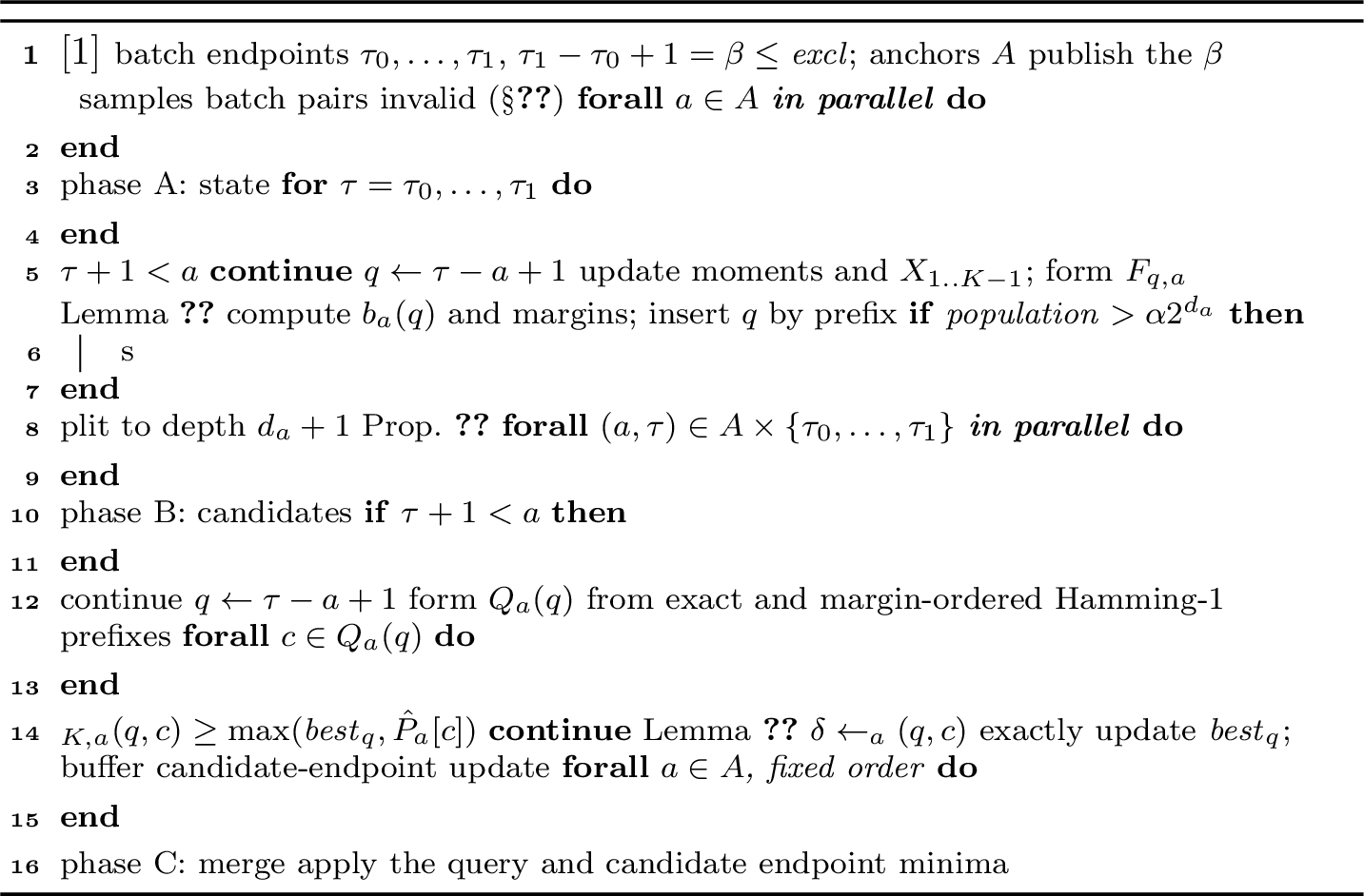
7 Update and Emit Pseudocode↩︎
Algorithm 4 lists one batch of the streaming update (§3.5). Phase A advances every anchor’s sliding state and inserts the new signatures, splitting any directory whose population exceeds its occupancy bound (Prop. 4). Phase B forms candidates from the exact-prefix bucket and its margin-ordered Hamming-1 neighbors, rejects them with the Parseval bound (Lemma 2), computes exact distances for the survivors, and buffers the cell updates privately. Phase C merges the buffers in a fixed order, which is what makes the output independent of the thread schedule (Prop. 5). Algorithm 5 lists the emit stage (§3.6). It runs the hot-class sieve, then refinement to a fixpoint, then the final zero-snap and top-\(k\) selection. As throughout, \(R=\gamma\alpha\) is the per-query verification budget.
8 Notation↩︎
Table 1 collects the symbols used throughout the paper. Calligraphic letters denote sets of comparison triples, and hatted symbols denote maintained quantities, as opposed to their exact counterparts.
| \(T\), \(n\) | time series and its length |
| \(m\in[m_{\min},m_{\max}]\), \(L\) | window length; interval size |
| \(T_{i,m}\), \(Z_{i,m}\) | window at start \(i\); its z-normalized form |
| \(\dist_m(i,j)\) | z-normalized Euclidean distance |
| \(\mathit{excl}\) | exclusion radius for valid pairs |
| \(P_m\), \(I_m\); \(\hat P_m\), \(\hat I_m\) | exact and maintained profile rows |
| \(\mathcal U\); \(\mathcal S\); \(P^{\mathcal S}\) | comparison universe; evaluated set; induced profile |
| \(\tau\); \(q\) | stream time (latest sample); window start |
| \(A\), \(a\), \(s\) | anchor set; an anchor length; anchor stride |
| \(K\), \(K'\) | retained spectral width; aliasing-safe cap |
| \(F_{i,m}\) | normalized non-DC spectral feature vector |
| \(\pbound_{K,m}(i,j)\) | Parseval lower bound on \(\dist_m(i,j)\) |
| \(B\); \(b_a(i)\); \(g_{a,\ell}\) | signature width; a signature; a projection |
| \(d\), \(d_0\) | directory depth; probe reference depth |
| \(\alpha\); \(\gamma\); \(R=\gamma\alpha\) | occupancy target; multiplier; verification budget |
| \(\beta\) | micro-batch size (\(\beta\le\mathit{excl}\)) |
| \(w\) | sieve neighbor width |
| \(\Delta_m\), \(\Delta_p\), \(P_{\max}\) | refinement radii and round cap |
| \(\eta\); \(\theta_K\) | energy-capture threshold; sampled feature angle |
| \(\lambda\); \(\varepsilon_0\) | bound shrink factor; zero-snap threshold |
| \(\varphi\) | fraction of candidates reaching exact evaluation |
9 Deferred Proofs↩︎
This appendix completes every claim the paper states without proof. Six statements of §3 defer their proofs here, one lemma appears here for the first time, and one step that §3.2 uses without derivation is carried out in full. Lemma 2 states that the truncated spectral sum of §3.2 never exceeds the exact z-normalized distance, and that the cap \(K'\) prevents a frequency bin and its mirror image from being counted twice when the window is shorter than twice the retained width. Proposition 2 states that no spectral width can invalidate an output, because the bound stays a lower bound at every width and a width change alters only the set of evaluated pairs. Proposition 4 states that splitting a directory whenever its population crosses the occupancy threshold keeps the mean bucket size near the target \(\alpha\), at rehoming cost that amortizes to a constant per insertion. Proposition 3 states that the probability that every anchor misses a matchable pair is the product of the per-anchor miss probabilities, because each anchor draws its own projections. Lemma 3 states that the closest pair of a hot class lands within a few positions of each other when the class is sorted by one random projection. Proposition 5 states that the emitted motifs are identical for every thread count and schedule. The new statement is Lemma 4. The feature cache is the largest memory consumer (§3.7), so Panache stores features in single rather than double precision (§3.2). Rounding perturbs every stored coefficient, and a bound computed from perturbed features can come out larger than the true bound. Larger is the dangerous direction, since an overestimated lower bound could discard a pair whose exact distance would have survived the test. The implementation therefore shrinks every computed bound by \(1-\lambda\) before the comparison, and the lemma proves the shrink covers the rounding error whenever the bound is large enough to prune at all. Single precision halves the cache, and the bound stays a true lower bound. The proofs below derive every inequality they use. The uncovered step, the vanishing geometric sum in the proof of Lemma 1, is completed first.
Geometric sum in Lemma 1. The proof in §3.2 uses that \(G_{k,m}\), the sum of \(e^{-2\pi\mathrm{i}kr/m}\) over \(r=0,\ldots,m-1\), vanishes when \(k\not\equiv 0 \pmod m\). The sum is a geometric series with ratio \(q = e^{-2\pi\mathrm{i}k/m}\). For \(k \not\equiv 0 \pmod m\) the ratio satisfies \(q \ne 1\), so the series sums to \(G_{k,m} = (1-q^m)/(1-q)\), and \(q^m = e^{-2\pi\mathrm{i}k} = 1\) makes the numerator zero. Hence \(G_{k,m} = 0\). ◻
Lemma 4 (Quantized bound safety). With features stored at relative precision \(\varepsilon\), shrinking the computed bound by \((1 - \lambda)\) preserves Lemma 2 whenever the bound exceeds \(\sqrt{2m} \cdot 2\sqrt{2}\,\varepsilon / \lambda\).
Proof of Lemma 2. Let \(\hat{A}_k\) and \(\hat{B}_k\) be the DFT coefficients of the z-normalized windows \(Z_{i,m}\) and \(Z_{j,m}\), and write \(t_k = |\hat{A}_k - \hat{B}_k|^2\). Parseval’s theorem for the DFT states \[\mathrm{d}_m(i,j)^2 = \sum_{r=0}^{m-1} \bigl(Z_{i,m}[r]-Z_{j,m}[r]\bigr)^2 = \frac{1}{m}\sum_{k=0}^{m-1} t_k .\] Both windows have mean zero, so \(\hat{A}_0 = \hat{B}_0 = 0\) and \(t_0 = 0\). Both windows are real, so \(\hat{A}_{m-k} = \overline{\hat{A}_k}\) and \(\hat{B}_{m-k} = \overline{\hat{B}_k}\), and taking magnitudes gives \(t_{m-k} = t_k\) for \(1 \le k \le m-1\). Hence \[2\sum_{k=1}^{K'} t_k = \sum_{k=1}^{K'} \bigl(t_k + t_{m-k}\bigr).\] The cap \(K' \le \lceil m/2 \rceil - 1\) is equivalent to \(2K' < m\). Under it, the index sets \(\{1,\ldots,K'\}\) and \(\{m{-}K',\ldots,m{-}1\}\) are disjoint subsets of \(\{1,\ldots,m{-}1\}\), so the right side above is a sum of \(2K'\) distinct terms of the full Parseval sum. Every \(t_k\) is nonnegative, so \[2\sum_{k=1}^{K'} t_k \;\le\; \sum_{k=0}^{m-1} t_k \;=\; m\,\mathrm{d}_m(i,j)^2 .\] By Lemma 1, the stored features equal the coefficients \(\hat{A}_k\) and \(\hat{B}_k\), so the left side equals \(m\,\underline{\mathrm{d}}_{K,m}^2(i,j)\) by the definition of the bound in §3.2. Dividing by \(m\) and taking square roots gives \(\underline{\mathrm{d}}_{K,m}(i,j) \le \mathrm{d}_m(i,j)\). ◻
Proof of Proposition 2. (i) In the proof of Lemma 2 above, \(m\,\underline{\mathrm{d}}_{K,m}^2(i,j)=2\sum_{k=1}^{K'}t_k\) is a sum of \(2K'\) distinct nonnegative terms of the full Parseval sum \(\sum_{k=0}^{m-1}t_k=m\,\mathrm{d}_m(i,j)^2\), and no step of that argument constrains \(K\). This proves the inequality for every \(K\ge 2\). For \(K_1\le K_2\) the caps satisfy \(K_1'\le K_2'\), and the sub-sum at \(K_2\) contains the sub-sum at \(K_1\) plus nonnegative terms, which proves the monotonicity. (ii) An evaluated pair’s exact distance is computed from raw samples and window moments in the closed form of §2. No write reads the features, and the features are read only to propose, filter, and order candidate pairs (§3.4, §3.6). A different width therefore changes only the evaluated set \(\mathcal{S}\), and Proposition 1 gives soundness for every \(\mathcal{S}\subseteq\mathcal{U}\). ◻
Proof of Proposition 4. Let \(P\) be the number of windows in one anchor’s directory and let \(d\) be its prefix depth. A further split is possible while \(d\) is smaller than the signature width \(B\), since deepening the prefix uses one signature bit beyond the current depth. While a split is possible, the split rule fires as soon as an insertion pushes \(P\) above \(\alpha 2^d\), so \(P \le \alpha 2^d\) holds after every insertion, and the mean bucket occupancy \(P/2^d\) is at most \(\alpha\). Before the first split the directory may be far below this bound. After the first split, the split that brought the directory to its current depth \(d\) fired because \(P\) exceeded \(\alpha 2^{d-1}\), and \(P\) never decreases, so \(\alpha 2^{d-1} < P \le \alpha 2^d\) and the mean occupancy lies in \((\alpha/2,\alpha]\). A doubling at depth \(d\) rehomes at most \(\alpha 2^d + 1\) entries. The split that reached the final depth \(D\) fired because the population then exceeded \(\alpha 2^{D-1}\), which is smaller than \(P_{\mathrm{final}}\), so the total rehoming work over all doublings is at most \[\sum_{j=1}^{D} \bigl(\alpha 2^j + 1\bigr) \;\le\; 2\alpha 2^{D} + D \;<\; 4\,P_{\mathrm{final}} + D .\] This is \(O(P_{\mathrm{final}})\) moves over \(P_{\mathrm{final}}\) insertions, which is \(O(1)\) amortized per insertion. Once \(d\) reaches the signature width or the implementation cap, no bit remains to split on, and no further occupancy guarantee is possible without raising that limit. ◻
Proof of Proposition 3. Consider a matchable pair. For each anchor \(a \in M_A\), let \(E_a\) be the event that anchor \(a\) discovers the pair, meaning that the two windows collide in anchor \(a\)’s directory and that the budgeted scan then retains the pair. By the definitions of \(p_a\) and \(c_a\) in the statement, \(\Pr[E_a] = p_a c_a\). Treat the series as given, so that the only remaining randomness is in the projections \(g_{a,\ell}\). Every quantity that determines \(E_a\) is a function of the data and of anchor \(a\)’s own projections \(g_{a,1},\ldots,g_{a,B}\) and of nothing else: the signatures of the two windows, the bucket each occupies, the other occupants of that bucket, and the scan’s deterministic selection within it all depend only on these (§3.4). The projection families of different anchors are drawn independently, so the events \(\{E_a\}_{a\in M_A}\) are functions of mutually independent random variables and are therefore mutually independent, and so are their complements. Hence \[\Pr\Bigl[\,\bigcap_{a\in M_A} E_a^{\mathrm{c}}\Bigr] \;=\; \prod_{a\in M_A}\Pr\bigl[E_a^{\mathrm{c}}\bigr] \;=\; \prod_{a\in M_A}\bigl(1-p_a c_a\bigr),\] which establishes the claimed bound. ◻
Proof of Lemma 3. Write \(p(y) = \langle g, y\rangle\) for the projection of a feature vector \(y\), so the sieve sorts the class by \(p\). A member \(x\) lands strictly between \(u\) and \(v\) in the sorted order exactly when \(p(x)\) lies strictly between \(p(u)\) and \(p(v)\), which happens exactly when \(p(x)-p(u) = \langle g, x-u\rangle\) and \(p(x)-p(v) = \langle g, x-v\rangle\) differ in sign. By Fact 1, this event has probability \(\angle(x{-}u,\,x{-}v)/\pi\) over the Gaussian draw of \(g\). That angle is the angle at which \(x\) sees the segment from \(u\) to \(v\). The segment has length \(\delta\), and \(x\) lies at distance at least \(r_x\) from both of its endpoints, so the angle is largest when both distances equal \(r_x\) exactly, the isosceles configuration with \(\sin(\theta/2) = \delta/2r_x\). The function \(\arcsin\) is convex on \([0,1]\) with \(\arcsin(0)=0\) and \(\arcsin(1)=\pi/2\), so \(\arcsin(z) \le (\pi/2)\,z\) there. The probability that \(x\) lands between the pair is therefore at most \[\frac{\theta}{\pi} \;\le\; \frac{2\arcsin(\delta/2r_x)}{\pi} \;\le\; \frac{2}{\pi}\cdot\frac{\pi}{2}\cdot\frac{\delta}{2r_x} \;=\; \frac{\delta}{2r_x} .\] Let \(N\) be the number of members landing strictly between \(u\) and \(v\). \(N\) is a sum of indicator variables, one per other member, so linearity of expectation gives the first claim, \[\mathbb{E}[N] \;\le\; \frac{\delta}{2}\sum_x \frac{1}{r_x} .\] If \(u\) and \(v\) are separated by more than \(w\) positions in the sorted order, then at least \(w\) members lie strictly between them, so that event implies \(N \ge w\). Outcomes with \(N \ge w\) contribute at least \(w\) to the expectation, and all other outcomes contribute at least zero, so \(\mathbb{E}[N] \ge w\Pr[N \ge w]\). Dividing by \(w\) gives the second claim, \(\Pr[N \ge w] \le \mathbb{E}[N]/w\). ◻
Proof of Lemma 4. Let \(a_k\) and \(b_k\) be the feature components of the two windows, let \(D^2 = \sum_k (a_k - b_k)^2\) be the true squared feature gap, and let \(\tilde{D}^2\) be the value computed from components stored with relative error at most \(\varepsilon\). The computed bound of §3.2 is \(\frac{2}{m}\tilde{D}^2\). A stored component equals its true value times \((1+\theta)\) with \(|\theta| \le \varepsilon\), so \[\bigl|(\tilde{a}_k - \tilde{b}_k) - (a_k - b_k)\bigr| \;\le\; \varepsilon\bigl(|a_k| + |b_k|\bigr).\] Squaring, each term of \(\tilde{D}^2\) differs from its true value by at most \(2\varepsilon (|a_k| + |b_k|) |a_k - b_k| + O(\varepsilon^2)\). Summing over \(k\) and applying the Cauchy–Schwarz inequality with \(S^2 = \sum_k (|a_k| + |b_k|)^2\) gives \[\bigl|\tilde{D}^2 - D^2\bigr| \;\le\; 2\varepsilon \sum_k (|a_k|+|b_k|)\,|a_k - b_k| + O(\varepsilon^2) \;\le\; 2\varepsilon S D + O(\varepsilon^2),\] so the relative error of \(\tilde{D}^2\) is at most \(2\varepsilon S / D\), and the shrink \((1-\lambda)\) absorbs it whenever \(D \ge 2\varepsilon S / \lambda\). The features are stored in single precision, so \(\varepsilon = 2^{-24}\), and the shrink in use is \(\lambda = 10^{-4}\) (§3.2), which makes the condition \(D \ge S/839\) up to rounding. A z-normalized window carries total spectral energy \[\sum_{k=0}^{m-1} |\hat{X}_k|^2 \;=\; m \sum_r Z[r]^2 \;=\; m^2,\] and the stored features cover at most one bin of each conjugate pair, so over the stored bins \(\sum_k |\hat{X}_k|^2 \le m^2/2\). Since \((|a_k|+|b_k|)^2 \le 2(a_k^2 + b_k^2)\), this gives \(S^2 \le 2\,(m^2/2 + m^2/2) = 2m^2\), so \(S \le \sqrt{2}\,m\) and the condition becomes \[\frac{2}{m} D^2 \;\ge\; \bigl(\sqrt{2m}/600\bigr)^2,\] the threshold of the lemma. Below the threshold the shrink no longer covers the relative error, and the guarantee degrades gracefully instead of failing. Dividing \(|\tilde{D}^2 - D^2| \le 2\varepsilon S D\) by \(\tilde{D}+D \ge D\) and scaling by \(\sqrt{2/m}\) bounds the absolute inflation of the computed bound by \(2\varepsilon S\sqrt{2/m} \le 4\sqrt{m}\, \varepsilon\), which is below \(2.2\cdot10^{-6}\) at every benchmark length. A comparison misjudged below the threshold therefore leaves the affected cell within \(2.2\cdot10^{-6}\) of its exact value, an error of the same order as the zero-snap threshold \(\varepsilon_0=10^{-6}\) (§3.6) and below every precision at which distances are reported in this paper. ◻
Proof of Proposition 5. Fix the input stream, the configuration, and the seed. It suffices to show that the memory state after each batch is a function of the state before it and the batch contents alone, with no dependence on thread count or schedule, and that the emit stage is deterministic given that state.
Within one batch (Algorithm 4), the phase-A workers advance the online state of §3.2, and each worker owns one anchor’s moments, coefficients, and directory. No two workers touch the same memory, and writes to disjoint memory commute, so the state after phase A is the same set of per-anchor updates under every interleaving. The barrier between the phases guarantees that no phase-B unit starts before every phase-A write has completed, so each phase-B unit reads the same post-A state under every schedule. Phase B runs one work unit per new window, and the set of units is fixed by the batch contents, not by the schedule. Each unit probes the directory, rejects candidates with the Parseval bound, and evaluates the survivors exactly, all deterministic functions of the post-A state and the unit’s identity, and it records the resulting cell improvements only in its own private buffer. The buffer contents after phase B are therefore identical for every schedule. Phase C merges the buffers into the shared profile sequentially, in an order fixed by anchor and buffer index. Its inputs are schedule-independent and its order is fixed, so the resulting profile is as well. The min-updates use strict inequality, so a cell changes only when the new distance is strictly smaller. When two buffered improvements tie, the one merged first is kept, and the fixed merge order determines which one that is, so ties resolve identically on every run.
The state after a batch is therefore a function only of the state before it and the batch contents. The initial state is fixed by the configuration and the seed, and induction over the batches extends the identity to the state after the whole stream. In the emit stage, the hot-class sweep parallelizes only across anchors, and each anchor’s sweep writes only that anchor’s own profile rows, so the disjoint-memory argument of phase A applies unchanged. Local completion, the zero-snap of §3.6, and the final top-\(k\) selection run sequentially in a fixed order on this schedule-independent state. The emitted motifs are therefore identical for every thread count and schedule. ◻
10 Per-Row Recovery Composition↩︎
Table ¿tbl:tab:recovery-stats? decomposes the top-20 recovery of Table ¿tbl:tab:master? for the twenty rows scored against the exact Scamp-GPU reference, the \(\dagger\)-rows of Table ¿tbl:tab:master?. For each row, the reference list is the top-20 motifs of that exact reference, and the emitted list is the top-20 that Panache reports; recovery scoring (§4) pairs them. As defined there, a reference motif is a position match when Panache reports a start within \(m/2\) of the reference start at the same length, and a value match when it is not a position match but Panache reports that length’s best distance within the tolerance of §4, \(5\%\) relative or \(0.05\) absolute. The table gives, per row, the count of each, the smallest distance in the reference list (ref.best), and the largest gap between the two lists compared rank by rank: for each rank \(r\) in \(1,\ldots,20\) the absolute difference between the \(r\)-th smallest emitted distance and the \(r\)-th smallest reference distance, reported over the twenty ranks both in absolute form and relative to the reference distance at that rank.
Two facts explain every value match in the table, that is, every reference motif that Panache recovers by distance but not by position. First, several reference lists consist partly or wholly of distance-zero cells (ref.best \(=0\)). A distance-zero cell is a motif whose two windows have z-normalized distance exactly zero (§2), so they have identical normalized shape and are duplicates of each other. When a window has several duplicates its nearest neighbor is not unique, more than one start is an equally valid motif, and the reference and Panache may report different ones while their distances agree to below \(10^{-3}\). Such a row also has no meaningful relative error, since dividing by a zero reference distance is undefined, which is why §4 admits an absolute tolerance. The tiled Wafer rows are the extreme case. Past its natural 152k length Wafer is extended by repeating the series (§[sec:setup]), so every window has an exact copy, every top-20 motif sits at distance zero, and recovery is value-based by construction. Second, on rows whose reference distances are nonzero, a value match is a near-miss: Panache reports the motif a few positions from the reference start, at a distance that matches within tolerance. Across the twenty rows the largest rank-wise relative gap is 10.8% (TwoLeadECG) and the largest absolute gap is 0.0102 (ECG200), both inside the §4 tolerances. Every reference motif in the table is therefore accounted for as a position match, a duplicate-window tie counted by value, or a near-miss within tolerance.
3.6pt
@lrrrrrr@ Dataset & \(n\) & pos & val & ref.best & \(\max|\Delta\dist|\) & \(\max\) rel.
ItalyPowerDemand & 1,608 & 20 & 0 & 0.0432 & \(3.3{\cdot}10^{-6}\) & \(<0.1\%\)
ECG200 & 9,600 & 16 & 4 & 0.1846 & 0.0102 & 5.3%
TwoLeadECG & 93,398 & 12 & 8 & 0.0413 & 0.0045 & 10.8%
Wafer & 152,000 & 0 & 20 & 0 & 0 & –
Earthquakes & 164,864 & 19 & 1 & 0 & 0 & –
ECG5000 & 630,000 & 8 & 12 & 0.0889 & 0.0063 & 7.0%
ChlorineConc. & 637,440 & 3 & 17 & 0 & \(4.0{\cdot}10^{-4}\) & –
FordA & 660,000 & 13 & 7 & 0.0508 & 0.0049 & 8.3%
StarLightCurves & 1M & 1 & 19 & 0 & \(9.3{\cdot}10^{-4}\) & –
Mallat & 1M & 0 & 20 & 0 & 0 & –
Wafer & 8k & 17 & 3 & 0 & 0 & –
Wafer & 16k & 17 & 3 & 0 & 0 & –
Wafer & 32k & 19 & 1 & 0 & 0 & –
Wafer & 64k & 10 & 10 & 0 & 0 & –
Wafer (6 rows) & 128k–5M & 0 & 20 & 0 & 0 & –
11 Parameter Study↩︎
This study reruns the complete benchmark of Table ¿tbl:tab:master? while changing one design constant at a time. Every configuration covers all 37 reported rows, is scored against the same ground truth as §4, and runs on a c3-standard-44 instance with the fixed seed of the reference implementation, so every run is deterministic and every difference between configurations is caused by the changed constant. The control
configuration is unmodified Panache; it reproduces Table ¿tbl:tab:master? exactly, with 740 of 740 motifs recovered and 310 of 340 exact positions on the seventeen rows with exact Stumpy ground truth.
Every runtime in this study is a full-materialization time, the t.mat.accounting of Table ¿tbl:tab:master?. Each run executes the emit stage of §3.6 and writes every profile row, so that the complete output can be checked cell by cell against ground truth, which recovery scoring requires. The materialization work is identical in every configuration, so every ratio below divides two such runs, the shared cost cancels, and the ratio isolates the changed constant.
Tables ¿tbl:tab:abl-stride?–¿tbl:tab:abl-alpha? report every benchmark row under every setting. Cells follow the format of Table ¿tbl:tab:master?. Each cell gives the recovered top-20 motifs with their split into position and value matches, and the runtime in seconds.
The most important takeaway of this section is that changing a design constant does not affect recovery. Only runtime responds. All 22 single-constant settings recover 740 of 740 motifs, and their exact-position count, out of 340, never differs from the control’s by more than 15. Figure 6 plots the runtime response. Table 2 summarizes the study.
11.0.0.1 Anchor stride (Table ¿tbl:tab:abl-stride?).
Anchors index every \(s\)-th length and leave the remaining lengths to local completion (§3.3). Dense indexing (\(s=1\)) maintains a window and a directory at every length and recovers the same 740 motifs at \(1.92\times\) the total runtime; at Wafer 5M it takes 714 s against 363 s for the default. Coarser strides cut runtime further. At \(s=8\) the benchmark completes at \(0.37\times\) the control (130 s at 5M) and still recovers every motif, with exact positions within 4 of the control. Recovery does not depend on the stride anywhere in the swept range; only cost does.
11.0.0.2 Sieve width (Table ¿tbl:tab:abl-w?).
The sieve evaluates each member of an over-budget bucket against its \(w\) nearest neighbors in the projection order (§3.6). It costs at most 2% of total runtime at any width, so this sweep isolates quality. Every width recovers 740 of 740, and widths above the default add up to 13 exact positions (323 of 340 at \(w=32\)). The one visible per-row effect is StarLightCurves 64k, where \(w=2\) yields 18 exact positions and \(w\ge 8\) yields all 20.
11.0.0.3 Refinement radii (Table ¿tbl:tab:abl-radii?).
Local completion evaluates a box of \(\Delta_m\) lengths and \(\Delta_p\) starts around each seed (§3.6). Recovery and runtime are unchanged from \((2,1)\) to \((12,8)\), and positions move by at most two matches. Any radius that reaches the adjacent non-anchor lengths suffices. The neighborhood size is not a sensitive quantity.
11.0.0.4 Refinement rounds (Table ¿tbl:tab:abl-passes?).
Refinement repeats until no cell improves, capped at \(P_{\max}\) rounds (§3.6). Exact positions are identical for every cap \(P_{\max}\ge 1\). Refinement converges in one round on every benchmark row, and later rounds only re-verify. A cap of one round completes the benchmark at \(0.58\times\) the control (200 s against 362 s at Wafer 5M). The default cap of eight is a safety margin for streams where one round does not suffice, not a tuned value.
11.0.0.5 Occupancy target (Table ¿tbl:tab:abl-alpha?).
The target \(\alpha\) sets the bucket size the directory maintains, and the verification budget is \(R=8\alpha\) (§3.4). \(\alpha\) is the one parameter exposed to the analyst, and this sweep bounds its risk in both directions. A quarter of the default verification budget (\(\alpha=4\), \(R=32\)) still recovers 740 of 740 at \(0.74\times\) runtime, and four times the default (\(\alpha=64\)) buys 10 additional exact positions at \(1.94\times\). Mis-setting the only exposed knob by a factor of four in either direction costs no motif.
11.0.0.6 Spectral width (Table ¿tbl:tab:abl-kwidth?).
The width \(K\) is the one constant the calibration of §3.2 sets from data, so this sweep overrides it with fixed widths across the admissible range, \(K\in\{4,8,12,16\}\), in a dedicated session on the same machine type. Proposition 2 states that no width can invalidate an output, and the sweep is the matching measurement for coverage. Recovery is 740 of 740 at every sampled width from the three-bin bound at \(K=4\) to the full sixteen, exact positions stay within 6 of the control, and runtime falls as the width narrows, to \(0.81\times\) at \(K=4\), where the looser bound performs \(1.41\times\) the exact evaluations but every slide, signature, and stored feature is cheaper. The width moves speed, never discovery. The implementation floors the width at 4, below which the \(B\) signature bits would span too few feature dimensions to control bucket occupancy (§3.4).
11.0.0.7 Maximum performance (Table ¿tbl:tab:abl-maxperf?).
Each sweep above moves one constant and holds the rest at their defaults, so the fastest settings never meet in a single run. The maximum-performance configuration combines them, taking the fastest settings that jointly hold full recovery: anchor stride \(s=6\), occupancy target \(\alpha=4\), and round cap \(P_{\max}=1\). The radii stay at \((\Delta_m,\Delta_p)=(6,4)\) because a stride of six places non-anchor lengths up to three positions from the nearest anchor, and any \(\Delta_m\) below three would leave those lengths outside every completion box. The sieve width stays at \(w=8\) because the width sweep shows no runtime response. Table ¿tbl:tab:abl-maxperf? reports this configuration against the control, both measured in one session on a fresh instance of the benchmark machine type. The session is directly comparable to the sweeps. The control rerun reproduced every recovery, position, and value count of the sweep session from a byte-identical binary, and its total runtime moved by half a percent. The combined configuration recovers all 740 motifs at \(5.9\times\) lower total runtime, 139 s against 823 s across the benchmark. Wafer 5M completes in 52.1 s against 362 s, and StarLightCurves 1M in 10.1 s against 53.1 s. Exact positions are 308 of 340 against the control’s 310. The cost of the speed is two positions and no motif.
A final configuration pushes the combination to the floor of the width range. Taking \(\alpha=4\) and \(P_{\max}=1\) at the more aggressive stride \(s=8\) and fixing \(K=4\) trades the calibration’s collision headroom for speed on top of the quartered budget, the two thinnest margins in the design. The configuration recovers 740 of 740 motifs, at 104.3 s total against the control’s 823 s, a \(7.9\times\) reduction. Wafer 5M completes in 38.2 s against 362 s. Exact positions are 292 of 340. This configuration was measured in its own session on a fresh instance of the same machine type from a byte-identical binary. Its outputs are deterministic (Prop. 5), and the control totals reproduced across sessions within half a percent.
Table 2 condenses the study. The sweeps were run after every default was fixed and did not inform any default. Tuning constants from prior analysis of the benchmark datasets is not part of the study design. Staying faithful to that design, we report the conservative configuration in Table ¿tbl:tab:master?, although the maximum-performance configuration of Table ¿tbl:tab:abl-maxperf? delivers the same recovery at a further \(7.9\times\) lower runtime.
Figure 6: 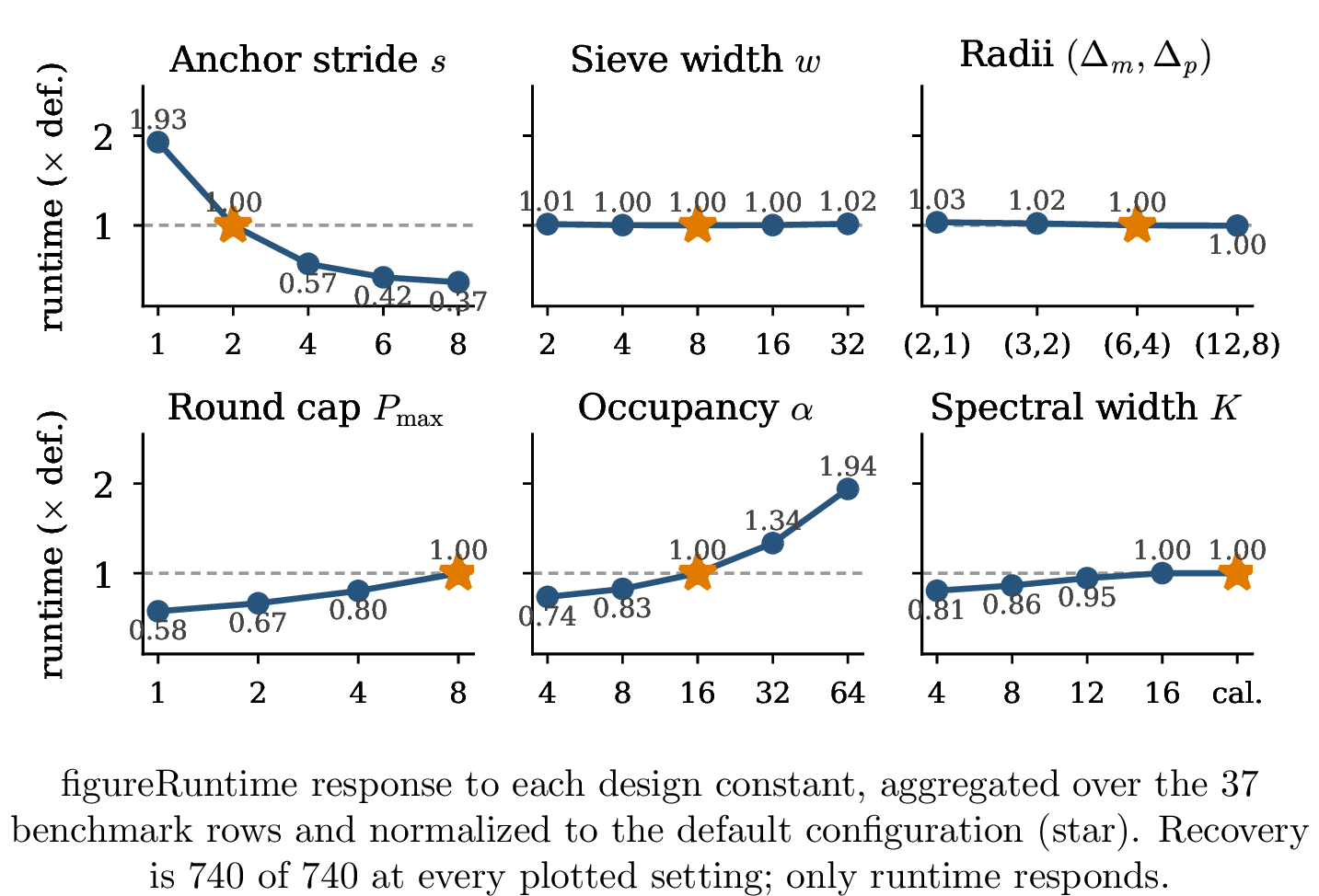 .
.
| Constant | Setting | Rec. | Pos. | Time |
|---|---|---|---|---|
| Anchor stride \(s\) | 1 (dense) | 740 | 313 | \(1.92\times\) |
| (§[sec:sec:anchors]) | \(2^\star\) | 740 | 310 | \(1.00\times\) |
| 4 | 740 | 305 | \(0.58\times\) | |
| 6 | 740 | 306 | \(0.43\times\) | |
| 8 | 740 | 306 | \(0.37\times\) | |
| Sieve width \(w\) | 2 | 740 | 306 | \(1.02\times\) |
| (§[sec:sec:emit]) | 4 | 740 | 310 | \(1.00\times\) |
| \(8^\star\) | 740 | 310 | \(1.00\times\) | |
| 16 | 740 | 314 | \(1.01\times\) | |
| 32 | 740 | 323 | \(1.02\times\) | |
| Radii \((\Delta_m,\Delta_p)\) | \((2,1)\) | 740 | 308 | \(1.05\times\) |
| (§[sec:sec:emit]) | \((3,2)\) | 740 | 308 | \(1.02\times\) |
| \((6,4)^\star\) | 740 | 310 | \(1.00\times\) | |
| \((12,8)\) | 740 | 310 | \(1.00\times\) | |
| Round cap \(P_{\max}\) | 1 | 740 | 310 | \(0.58\times\) |
| (§[sec:sec:emit]) | 2 | 740 | 310 | \(0.67\times\) |
| 4 | 740 | 310 | \(0.81\times\) | |
| \(8^\star\) | 740 | 310 | \(1.00\times\) | |
| Occupancy \(\alpha\) | 4 | 740 | 306 | \(0.74\times\) |
| (§[sec:sec:hashing]) | 8 | 740 | 306 | \(0.83\times\) |
| \(16^\star\) | 740 | 310 | \(1.00\times\) | |
| 32 | 740 | 319 | \(1.34\times\) | |
| 64 | 740 | 320 | \(1.93\times\) | |
| Spectral width \(K\) | 4 | 740 | 315 | \(0.81\times\) |
| (§[sec:sec:spectra]) | 8 | 740 | 310 | \(0.87\times\) |
| 12 | 740 | 315 | \(0.96\times\) | |
| 16 | 740 | 316 | \(1.00\times\) | |
| calibrated\(^\star\) | 740 | 310 | \(1.00\times\) |
@llrrrrrrrrrr@ Dataset & \(n\) & & & & &
& & rec (p+v) & t(s) & rec (p+v) & t(s) & rec (p+v) & t(s) & rec (p+v) & t(s) & rec (p+v) & t(s)
ECG200 & 8k & 20 (16+4) & 0.25 & 20 (16+4) & 0.14 & 20 (16+4) & 0.10 & 20 (16+4) & 0.08 & 20 (16+4) & 0.07
ItalyPowerDemand & 1,600 & 20 (20+0) & 0.03 & 20 (20+0) & 0.02 & 20 (20+0) & 0.02 & 20 (20+0) & 0.02 & 20 (20+0) & 0.02
Wafer & 8k & 20 (19+1) & 0.36 & 20 (19+1) & 0.25 & 20 (19+1) & 0.20 & 20 (19+1) & 0.14 & 20 (19+1) & 0.14
Earthquakes & 8k & 20 (20+0) & 0.47 & 20 (20+0) & 0.25 & 20 (20+0) & 0.16 & 20 (20+0) & 0.13 & 20 (20+0) & 0.11
StarLightCurves & 8k & 20 (20+0) & 0.41 & 20 (20+0) & 0.23 & 20 (20+0) & 0.15 & 20 (20+0) & 0.12 & 20 (20+0) & 0.12
ChlorineConc. & 8k & 20 (20+0) & 0.29 & 20 (20+0) & 0.22 & 20 (20+0) & 0.14 & 20 (20+0) & 0.11 & 20 (20+0) & 0.12
TwoLeadECG & 8k & 20 (20+0) & 0.26 & 20 (20+0) & 0.15 & 20 (20+0) & 0.11 & 20 (20+0) & 0.09 & 20 (20+0) & 0.08
ECG5000 & 8k & 20 (20+0) & 0.30 & 20 (20+0) & 0.14 & 20 (17+3) & 0.11 & 20 (17+3) & 0.08 & 20 (17+3) & 0.08
FordA & 8k & 20 (20+0) & 0.37 & 20 (20+0) & 0.20 & 20 (20+0) & 0.13 & 20 (20+0) & 0.11 & 20 (20+0) & 0.11
Mallat & 8k & 20 (13+7) & 0.37 & 20 (15+5) & 0.21 & 20 (15+5) & 0.19 & 20 (15+5) & 0.13 & 20 (15+5) & 0.10
ChlorineConc. & 64k & 20 (20+0) & 3.54 & 20 (20+0) & 2.27 & 20 (20+0) & 1.33 & 20 (20+0) & 0.99 & 20 (20+0) & 0.85
Earthquakes & 64k & 20 (20+0) & 5.11 & 20 (20+0) & 2.68 & 20 (20+0) & 1.50 & 20 (20+0) & 1.15 & 20 (20+0) & 1.42
ECG5000 & 64k & 20 (12+8) & 4.07 & 20 (12+8) & 2.08 & 20 (6+14) & 1.19 & 20 (6+14) & 0.91 & 20 (6+14) & 1.39
FordA & 64k & 20 (20+0) & 3.85 & 20 (15+5) & 1.97 & 20 (19+1) & 1.16 & 20 (20+0) & 1.03 & 20 (20+0) & 0.90
Mallat & 64k & 20 (17+3) & 8.02 & 20 (17+3) & 4.03 & 20 (17+3) & 2.21 & 20 (17+3) & 1.64 & 20 (17+3) & 1.39
StarLightCurves & 64k & 20 (20+0) & 4.31 & 20 (20+0) & 2.20 & 20 (20+0) & 1.29 & 20 (20+0) & 0.99 & 20 (20+0) & 0.97
Wafer & 64k & 20 (16+4) & 3.89 & 20 (16+4) & 1.99 & 20 (16+4) & 1.16 & 20 (16+4) & 0.89 & 20 (16+4) & 0.76
ItalyPowerDemand & 1,608 & 20 (20+0) & 0.03 & 20 (20+0) & 0.02 & 20 (20+0) & 0.02 & 20 (20+0) & 0.02 & 20 (20+0) & 0.02
ECG200 & 9,600 & 20 (16+4) & 0.30 & 20 (16+4) & 0.17 & 20 (16+4) & 0.12 & 20 (16+4) & 0.10 & 20 (16+4) & 0.09
TwoLeadECG & 93,398 & 20 (12+8) & 4.42 & 20 (12+8) & 2.38 & 20 (2+18) & 1.47 & 20 (8+12) & 1.09 & 20 (8+12) & 1.05
Wafer & 152k & 20 (0+20) & 11.5 & 20 (0+20) & 5.98 & 20 (0+20) & 3.41 & 20 (0+20) & 2.58 & 20 (0+20) & 2.20
Earthquakes & 164,864 & 20 (19+1) & 13.5 & 20 (19+1) & 7.06 & 20 (19+1) & 4.18 & 20 (19+1) & 3.56 & 20 (19+1) & 2.66
ECG5000 & 630k & 20 (8+12) & 36.8 & 20 (8+12) & 19.6 & 20 (8+12) & 12.5 & 20 (6+14) & 9.02 & 20 (6+14) & 8.81
ChlorineConc. & 637,440 & 20 (3+17) & 52.7 & 20 (3+17) & 31.8 & 20 (3+17) & 18.6 & 20 (3+17) & 13.8 & 20 (3+17) & 11.9
FordA & 660k & 20 (13+7) & 65.1 & 20 (13+7) & 33.6 & 20 (13+7) & 19.5 & 20 (13+7) & 16.3 & 20 (13+7) & 13.9
StarLightCurves & 1M & 20 (1+19) & 88.3 & 20 (1+19) & 53.1 & 20 (1+19) & 30.7 & 20 (1+19) & 22.6 & 20 (1+19) & 19.6
Mallat & 1M & 20 (0+20) & 68.6 & 20 (0+20) & 35.9 & 20 (0+20) & 21.3 & 20 (0+20) & 16.6 & 20 (0+20) & 14.6
Wafer & 8k & 20 (17+3) & 0.36 & 20 (17+3) & 0.24 & 20 (17+3) & 0.20 & 20 (17+3) & 0.14 & 20 (17+3) & 0.14
Wafer & 16k & 20 (17+3) & 0.60 & 20 (17+3) & 0.41 & 20 (17+3) & 0.25 & 20 (17+3) & 0.20 & 20 (17+3) & 0.18
Wafer & 32k & 20 (19+1) & 1.73 & 20 (19+1) & 0.89 & 20 (19+1) & 0.53 & 20 (19+1) & 0.42 & 20 (19+1) & 0.38
Wafer & 64k & 20 (10+10) & 3.85 & 20 (10+10) & 2.03 & 20 (10+10) & 1.15 & 20 (10+10) & 0.89 & 20 (10+10) & 0.75
Wafer & 128k & 20 (0+20) & 7.56 & 20 (0+20) & 4.75 & 20 (0+20) & 2.72 & 20 (0+20) & 2.05 & 20 (0+20) & 1.79
Wafer & 256k & 20 (0+20) & 29.4 & 20 (0+20) & 15.0 & 20 (0+20) & 8.47 & 20 (0+20) & 6.26 & 20 (0+20) & 5.27
Wafer & 512k & 20 (0+20) & 59.2 & 20 (0+20) & 30.4 & 20 (0+20) & 17.4 & 20 (0+20) & 12.7 & 20 (0+20) & 11.2
Wafer & 1M & 20 (0+20) & 123 & 20 (0+20) & 62.7 & 20 (0+20) & 36.3 & 20 (0+20) & 27.0 & 20 (0+20) & 22.4
Wafer & 2M & 20 (0+20) & 264 & 20 (0+20) & 133 & 20 (0+20) & 77.7 & 20 (0+20) & 56.2 & 20 (0+20) & 48.1
Wafer & 5M & 20 (0+20) & 714 & 20 (0+20) & 363 & 20 (0+20) & 207 & 20 (0+20) & 152 & 20 (0+20) & 130
@llrrrrrrrrrr@ Dataset & \(n\) & & & & &
& & rec (p+v) & t(s) & rec (p+v) & t(s) & rec (p+v) & t(s) & rec (p+v) & t(s) & rec (p+v) & t(s)
ECG200 & 8k & 20 (16+4) & 0.14 & 20 (16+4) & 0.14 & 20 (16+4) & 0.14 & 20 (16+4) & 0.14 & 20 (20+0) & 0.15
ItalyPowerDemand & 1,600 & 20 (18+2) & 0.02 & 20 (20+0) & 0.02 & 20 (20+0) & 0.02 & 20 (20+0) & 0.02 & 20 (20+0) & 0.02
Wafer & 8k & 20 (19+1) & 0.24 & 20 (19+1) & 0.24 & 20 (19+1) & 0.25 & 20 (19+1) & 0.25 & 20 (19+1) & 0.24
Earthquakes & 8k & 20 (20+0) & 0.25 & 20 (20+0) & 0.25 & 20 (20+0) & 0.25 & 20 (20+0) & 0.25 & 20 (20+0) & 0.25
StarLightCurves & 8k & 20 (20+0) & 0.23 & 20 (20+0) & 0.23 & 20 (20+0) & 0.23 & 20 (20+0) & 0.23 & 20 (20+0) & 0.23
ChlorineConc. & 8k & 20 (20+0) & 0.21 & 20 (20+0) & 0.21 & 20 (20+0) & 0.22 & 20 (20+0) & 0.22 & 20 (20+0) & 0.21
TwoLeadECG & 8k & 20 (20+0) & 0.15 & 20 (20+0) & 0.15 & 20 (20+0) & 0.15 & 20 (20+0) & 0.15 & 20 (20+0) & 0.16
ECG5000 & 8k & 20 (20+0) & 0.14 & 20 (20+0) & 0.14 & 20 (20+0) & 0.14 & 20 (20+0) & 0.14 & 20 (20+0) & 0.14
FordA & 8k & 20 (20+0) & 0.22 & 20 (20+0) & 0.20 & 20 (20+0) & 0.20 & 20 (20+0) & 0.21 & 20 (20+0) & 0.21
Mallat & 8k & 20 (15+5) & 0.21 & 20 (15+5) & 0.21 & 20 (15+5) & 0.21 & 20 (15+5) & 0.22 & 20 (15+5) & 0.21
ChlorineConc. & 64k & 20 (20+0) & 2.23 & 20 (20+0) & 2.29 & 20 (20+0) & 2.27 & 20 (20+0) & 2.24 & 20 (20+0) & 2.27
Earthquakes & 64k & 20 (20+0) & 2.67 & 20 (20+0) & 2.65 & 20 (20+0) & 2.68 & 20 (20+0) & 2.63 & 20 (20+0) & 2.63
ECG5000 & 64k & 20 (10+10) & 2.11 & 20 (10+10) & 2.07 & 20 (12+8) & 2.08 & 20 (12+8) & 2.15 & 20 (16+4) & 2.13
FordA & 64k & 20 (17+3) & 1.98 & 20 (17+3) & 2.41 & 20 (15+5) & 1.97 & 20 (19+1) & 2.02 & 20 (20+0) & 2.02
Mallat & 64k & 20 (17+3) & 4.01 & 20 (17+3) & 4.01 & 20 (17+3) & 4.03 & 20 (17+3) & 4.00 & 20 (17+3) & 4.18
StarLightCurves & 64k & 20 (18+2) & 2.59 & 20 (20+0) & 2.61 & 20 (20+0) & 2.20 & 20 (20+0) & 2.26 & 20 (20+0) & 2.26
Wafer & 64k & 20 (16+4) & 1.98 & 20 (16+4) & 1.99 & 20 (16+4) & 1.99 & 20 (16+4) & 2.04 & 20 (16+4) & 2.01
ItalyPowerDemand & 1,608 & 20 (18+2) & 0.02 & 20 (20+0) & 0.02 & 20 (20+0) & 0.02 & 20 (20+0) & 0.02 & 20 (20+0) & 0.02
ECG200 & 9,600 & 20 (16+4) & 0.17 & 20 (16+4) & 0.17 & 20 (16+4) & 0.17 & 20 (16+4) & 0.18 & 20 (20+0) & 0.18
TwoLeadECG & 93,398 & 20 (12+8) & 2.28 & 20 (12+8) & 2.30 & 20 (12+8) & 2.38 & 20 (12+8) & 2.33 & 20 (13+7) & 2.38
Wafer & 152k & 20 (0+20) & 5.95 & 20 (0+20) & 5.96 & 20 (0+20) & 5.98 & 20 (0+20) & 6.05 & 20 (0+20) & 6.04
Earthquakes & 164,864 & 20 (19+1) & 7.16 & 20 (19+1) & 7.06 & 20 (19+1) & 7.06 & 20 (19+1) & 7.03 & 20 (19+1) & 7.07
ECG5000 & 630k & 20 (8+12) & 19.5 & 20 (8+12) & 19.7 & 20 (8+12) & 19.6 & 20 (12+8) & 20.0 & 20 (12+8) & 20.0
ChlorineConc. & 637,440 & 20 (3+17) & 31.9 & 20 (3+17) & 31.8 & 20 (3+17) & 31.8 & 20 (3+17) & 32.6 & 20 (3+17) & 32.4
FordA & 660k & 20 (17+3) & 35.4 & 20 (17+3) & 33.6 & 20 (13+7) & 33.6 & 20 (18+2) & 33.7 & 20 (18+2) & 34.1
StarLightCurves & 1M & 20 (0+20) & 61.0 & 20 (0+20) & 53.1 & 20 (1+19) & 53.1 & 20 (1+19) & 53.6 & 20 (1+19) & 54.2
Mallat & 1M & 20 (0+20) & 36.1 & 20 (0+20) & 35.9 & 20 (0+20) & 35.9 & 20 (0+20) & 36.5 & 20 (0+20) & 36.9
Wafer & 8k & 20 (17+3) & 0.24 & 20 (17+3) & 0.24 & 20 (17+3) & 0.24 & 20 (17+3) & 0.24 & 20 (17+3) & 0.24
Wafer & 16k & 20 (17+3) & 0.41 & 20 (17+3) & 0.41 & 20 (17+3) & 0.41 & 20 (17+3) & 0.41 & 20 (17+3) & 0.41
Wafer & 32k & 20 (19+1) & 0.89 & 20 (19+1) & 0.89 & 20 (19+1) & 0.89 & 20 (19+1) & 0.75 & 20 (19+1) & 0.76
Wafer & 64k & 20 (10+10) & 2.00 & 20 (10+10) & 1.98 & 20 (10+10) & 2.03 & 20 (10+10) & 2.00 & 20 (10+10) & 2.01
Wafer & 128k & 20 (0+20) & 4.86 & 20 (0+20) & 4.78 & 20 (0+20) & 4.75 & 20 (0+20) & 4.83 & 20 (0+20) & 4.82
Wafer & 256k & 20 (0+20) & 15.1 & 20 (0+20) & 14.9 & 20 (0+20) & 15.0 & 20 (0+20) & 15.1 & 20 (0+20) & 15.2
Wafer & 512k & 20 (0+20) & 30.0 & 20 (0+20) & 30.1 & 20 (0+20) & 30.4 & 20 (0+20) & 32.2 & 20 (0+20) & 30.8
Wafer & 1M & 20 (0+20) & 63.5 & 20 (0+20) & 62.8 & 20 (0+20) & 62.7 & 20 (0+20) & 62.9 & 20 (0+20) & 63.5
Wafer & 2M & 20 (0+20) & 134 & 20 (0+20) & 134 & 20 (0+20) & 133 & 20 (0+20) & 134 & 20 (0+20) & 138
Wafer & 5M & 20 (0+20) & 364 & 20 (0+20) & 363 & 20 (0+20) & 363 & 20 (0+20) & 363 & 20 (0+20) & 367
@llrrrrrrrr@ Dataset & \(n\) & & & &
& & rec (p+v) & t(s) & rec (p+v) & t(s) & rec (p+v) & t(s) & rec (p+v) & t(s)
ECG200 & 8k & 20 (16+4) & 0.13 & 20 (16+4) & 0.13 & 20 (16+4) & 0.14 & 20 (16+4) & 0.22
ItalyPowerDemand & 1,600 & 20 (20+0) & 0.02 & 20 (20+0) & 0.02 & 20 (20+0) & 0.02 & 20 (20+0) & 0.06
Wafer & 8k & 20 (19+1) & 0.19 & 20 (19+1) & 0.19 & 20 (19+1) & 0.25 & 20 (19+1) & 0.36
Earthquakes & 8k & 20 (20+0) & 0.24 & 20 (20+0) & 0.20 & 20 (20+0) & 0.25 & 20 (20+0) & 0.36
StarLightCurves & 8k & 20 (20+0) & 0.21 & 20 (20+0) & 0.21 & 20 (20+0) & 0.23 & 20 (20+0) & 0.33
ChlorineConc. & 8k & 20 (20+0) & 0.19 & 20 (20+0) & 0.19 & 20 (20+0) & 0.22 & 20 (20+0) & 0.31
TwoLeadECG & 8k & 20 (20+0) & 0.16 & 20 (20+0) & 0.14 & 20 (20+0) & 0.15 & 20 (20+0) & 0.23
ECG5000 & 8k & 20 (18+2) & 0.13 & 20 (18+2) & 0.13 & 20 (20+0) & 0.14 & 20 (20+0) & 0.21
FordA & 8k & 20 (20+0) & 0.20 & 20 (20+0) & 0.21 & 20 (20+0) & 0.20 & 20 (20+0) & 0.29
Mallat & 8k & 20 (15+5) & 0.33 & 20 (15+5) & 0.27 & 20 (15+5) & 0.21 & 20 (15+5) & 0.32
ChlorineConc. & 64k & 20 (20+0) & 2.23 & 20 (20+0) & 2.23 & 20 (20+0) & 2.27 & 20 (20+0) & 2.41
Earthquakes & 64k & 20 (20+0) & 2.21 & 20 (20+0) & 3.07 & 20 (20+0) & 2.68 & 20 (20+0) & 2.29
ECG5000 & 64k & 20 (12+8) & 2.47 & 20 (12+8) & 2.49 & 20 (12+8) & 2.08 & 20 (12+8) & 2.17
FordA & 64k & 20 (15+5) & 2.78 & 20 (15+5) & 2.37 & 20 (15+5) & 1.97 & 20 (15+5) & 2.08
Mallat & 64k & 20 (17+3) & 3.96 & 20 (17+3) & 3.97 & 20 (17+3) & 4.03 & 20 (17+3) & 4.19
StarLightCurves & 64k & 20 (20+0) & 2.62 & 20 (20+0) & 2.59 & 20 (20+0) & 2.20 & 20 (20+0) & 2.29
Wafer & 64k & 20 (16+4) & 2.39 & 20 (16+4) & 1.97 & 20 (16+4) & 1.99 & 20 (16+4) & 2.07
ItalyPowerDemand & 1,608 & 20 (20+0) & 0.02 & 20 (20+0) & 0.02 & 20 (20+0) & 0.02 & 20 (20+0) & 0.06
ECG200 & 9,600 & 20 (16+4) & 0.16 & 20 (16+4) & 0.19 & 20 (16+4) & 0.17 & 20 (16+4) & 0.25
TwoLeadECG & 93,398 & 20 (12+8) & 2.72 & 20 (12+8) & 2.68 & 20 (12+8) & 2.38 & 20 (12+8) & 2.37
Wafer & 152k & 20 (0+20) & 5.98 & 20 (0+20) & 5.95 & 20 (0+20) & 5.98 & 20 (0+20) & 6.21
Earthquakes & 164,864 & 20 (19+1) & 7.04 & 20 (19+1) & 7.06 & 20 (19+1) & 7.06 & 20 (19+1) & 7.13
ECG5000 & 630k & 20 (8+12) & 25.3 & 20 (8+12) & 22.4 & 20 (8+12) & 19.6 & 20 (8+12) & 19.8
ChlorineConc. & 637,440 & 20 (3+17) & 31.8 & 20 (3+17) & 32.0 & 20 (3+17) & 31.8 & 20 (3+17) & 32.1
FordA & 660k & 20 (13+7) & 38.7 & 20 (13+7) & 38.8 & 20 (13+7) & 33.6 & 20 (13+7) & 33.8
StarLightCurves & 1M & 20 (1+19) & 77.0 & 20 (1+19) & 61.3 & 20 (1+19) & 53.1 & 20 (1+19) & 45.6
Mallat & 1M & 20 (0+20) & 35.9 & 20 (0+20) & 35.9 & 20 (0+20) & 35.9 & 20 (0+20) & 35.9
Wafer & 8k & 20 (17+3) & 0.20 & 20 (17+3) & 0.19 & 20 (17+3) & 0.24 & 20 (17+3) & 0.36
Wafer & 16k & 20 (17+3) & 0.39 & 20 (17+3) & 0.33 & 20 (17+3) & 0.41 & 20 (17+3) & 0.49
Wafer & 32k & 20 (19+1) & 0.91 & 20 (19+1) & 0.92 & 20 (19+1) & 0.89 & 20 (19+1) & 0.97
Wafer & 64k & 20 (10+10) & 2.36 & 20 (10+10) & 2.14 & 20 (10+10) & 2.03 & 20 (10+10) & 2.06
Wafer & 128k & 20 (0+20) & 4.74 & 20 (0+20) & 4.88 & 20 (0+20) & 4.75 & 20 (0+20) & 4.85
Wafer & 256k & 20 (0+20) & 15.0 & 20 (0+20) & 15.0 & 20 (0+20) & 15.0 & 20 (0+20) & 15.2
Wafer & 512k & 20 (0+20) & 30.2 & 20 (0+20) & 30.3 & 20 (0+20) & 30.4 & 20 (0+20) & 30.4
Wafer & 1M & 20 (0+20) & 62.6 & 20 (0+20) & 63.3 & 20 (0+20) & 62.7 & 20 (0+20) & 63.0
Wafer & 2M & 20 (0+20) & 134 & 20 (0+20) & 134 & 20 (0+20) & 133 & 20 (0+20) & 134
Wafer & 5M & 20 (0+20) & 363 & 20 (0+20) & 362 & 20 (0+20) & 363 & 20 (0+20) & 364
@llrrrrrrrr@ Dataset & \(n\) & & & &
& & rec (p+v) & t(s) & rec (p+v) & t(s) & rec (p+v) & t(s) & rec (p+v) & t(s)
ECG200 & 8k & 20 (16+4) & 0.09 & 20 (16+4) & 0.12 & 20 (16+4) & 0.15 & 20 (16+4) & 0.14
ItalyPowerDemand & 1,600 & 20 (20+0) & 0.01 & 20 (20+0) & 0.02 & 20 (20+0) & 0.02 & 20 (20+0) & 0.02
Wafer & 8k & 20 (19+1) & 0.12 & 20 (19+1) & 0.16 & 20 (19+1) & 0.24 & 20 (19+1) & 0.25
Earthquakes & 8k & 20 (20+0) & 0.12 & 20 (20+0) & 0.17 & 20 (20+0) & 0.25 & 20 (20+0) & 0.25
StarLightCurves & 8k & 20 (20+0) & 0.14 & 20 (20+0) & 0.18 & 20 (20+0) & 0.23 & 20 (20+0) & 0.23
ChlorineConc. & 8k & 20 (20+0) & 0.12 & 20 (20+0) & 0.16 & 20 (20+0) & 0.21 & 20 (20+0) & 0.22
TwoLeadECG & 8k & 20 (20+0) & 0.10 & 20 (20+0) & 0.13 & 20 (20+0) & 0.15 & 20 (20+0) & 0.15
ECG5000 & 8k & 20 (20+0) & 0.09 & 20 (20+0) & 0.12 & 20 (20+0) & 0.14 & 20 (20+0) & 0.14
FordA & 8k & 20 (20+0) & 0.11 & 20 (20+0) & 0.16 & 20 (20+0) & 0.21 & 20 (20+0) & 0.20
Mallat & 8k & 20 (15+5) & 0.12 & 20 (15+5) & 0.16 & 20 (15+5) & 0.21 & 20 (15+5) & 0.21
ChlorineConc. & 64k & 20 (20+0) & 1.43 & 20 (20+0) & 1.84 & 20 (20+0) & 2.27 & 20 (20+0) & 2.27
Earthquakes & 64k & 20 (20+0) & 1.39 & 20 (20+0) & 1.81 & 20 (20+0) & 2.68 & 20 (20+0) & 2.68
ECG5000 & 64k & 20 (12+8) & 1.30 & 20 (12+8) & 1.65 & 20 (12+8) & 2.09 & 20 (12+8) & 2.08
FordA & 64k & 20 (15+5) & 1.20 & 20 (15+5) & 1.57 & 20 (15+5) & 1.99 & 20 (15+5) & 1.97
Mallat & 64k & 20 (17+3) & 1.38 & 20 (17+3) & 1.74 & 20 (17+3) & 2.52 & 20 (17+3) & 4.03
StarLightCurves & 64k & 20 (20+0) & 1.37 & 20 (20+0) & 1.78 & 20 (20+0) & 2.24 & 20 (20+0) & 2.20
Wafer & 64k & 20 (16+4) & 1.18 & 20 (16+4) & 1.58 & 20 (16+4) & 2.04 & 20 (16+4) & 1.99
ItalyPowerDemand & 1,608 & 20 (20+0) & 0.01 & 20 (20+0) & 0.02 & 20 (20+0) & 0.02 & 20 (20+0) & 0.02
ECG200 & 9,600 & 20 (16+4) & 0.11 & 20 (16+4) & 0.15 & 20 (16+4) & 0.19 & 20 (16+4) & 0.17
TwoLeadECG & 93,398 & 20 (12+8) & 1.55 & 20 (12+8) & 1.93 & 20 (12+8) & 2.30 & 20 (12+8) & 2.38
Wafer & 152k & 20 (0+20) & 3.95 & 20 (0+20) & 4.96 & 20 (0+20) & 5.96 & 20 (0+20) & 5.98
Earthquakes & 164,864 & 20 (19+1) & 4.91 & 20 (19+1) & 5.93 & 20 (19+1) & 7.04 & 20 (19+1) & 7.06
ECG5000 & 630k & 20 (8+12) & 14.2 & 20 (8+12) & 16.8 & 20 (8+12) & 19.6 & 20 (8+12) & 19.6
ChlorineConc. & 637,440 & 20 (3+17) & 22.4 & 20 (3+17) & 27.3 & 20 (3+17) & 32.0 & 20 (3+17) & 31.8
FordA & 660k & 20 (13+7) & 23.4 & 20 (13+7) & 28.5 & 20 (13+7) & 33.6 & 20 (13+7) & 33.6
StarLightCurves & 1M & 20 (1+19) & 29.5 & 20 (1+19) & 37.6 & 20 (1+19) & 53.2 & 20 (1+19) & 53.1
Mallat & 1M & 20 (0+20) & 29.9 & 20 (0+20) & 35.8 & 20 (0+20) & 36.0 & 20 (0+20) & 35.9
Wafer & 8k & 20 (17+3) & 0.12 & 20 (17+3) & 0.16 & 20 (17+3) & 0.25 & 20 (17+3) & 0.24
Wafer & 16k & 20 (17+3) & 0.24 & 20 (17+3) & 0.33 & 20 (17+3) & 0.42 & 20 (17+3) & 0.41
Wafer & 32k & 20 (19+1) & 0.52 & 20 (19+1) & 0.70 & 20 (19+1) & 0.89 & 20 (19+1) & 0.89
Wafer & 64k & 20 (10+10) & 1.20 & 20 (10+10) & 1.58 & 20 (10+10) & 2.00 & 20 (10+10) & 2.03
Wafer & 128k & 20 (0+20) & 3.11 & 20 (0+20) & 3.95 & 20 (0+20) & 4.89 & 20 (0+20) & 4.75
Wafer & 256k & 20 (0+20) & 7.04 & 20 (0+20) & 8.29 & 20 (0+20) & 10.4 & 20 (0+20) & 15.0
Wafer & 512k & 20 (0+20) & 15.4 & 20 (0+20) & 17.7 & 20 (0+20) & 21.7 & 20 (0+20) & 30.4
Wafer & 1M & 20 (0+20) & 33.9 & 20 (0+20) & 37.5 & 20 (0+20) & 47.8 & 20 (0+20) & 62.7
Wafer & 2M & 20 (0+20) & 73.6 & 20 (0+20) & 81.5 & 20 (0+20) & 98.6 & 20 (0+20) & 133
Wafer & 5M & 20 (0+20) & 200 & 20 (0+20) & 223 & 20 (0+20) & 269 & 20 (0+20) & 363
@llrrrrrrrrrr@ Dataset & \(n\) & & & & &
& & rec (p+v) & t(s) & rec (p+v) & t(s) & rec (p+v) & t(s) & rec (p+v) & t(s) & rec (p+v) & t(s)
ECG200 & 8k & 20 (16+4) & 0.14 & 20 (16+4) & 0.14 & 20 (16+4) & 0.14 & 20 (20+0) & 0.15 & 20 (20+0) & 0.16
ItalyPowerDemand & 1,600 & 20 (19+1) & 0.02 & 20 (20+0) & 0.02 & 20 (20+0) & 0.02 & 20 (20+0) & 0.02 & 20 (20+0) & 0.02
Wafer & 8k & 20 (19+1) & 0.24 & 20 (19+1) & 0.24 & 20 (19+1) & 0.25 & 20 (19+1) & 0.25 & 20 (18+2) & 0.26
Earthquakes & 8k & 20 (20+0) & 0.20 & 20 (20+0) & 0.20 & 20 (20+0) & 0.25 & 20 (20+0) & 0.35 & 20 (20+0) & 0.38
StarLightCurves & 8k & 20 (20+0) & 0.21 & 20 (20+0) & 0.22 & 20 (20+0) & 0.23 & 20 (20+0) & 0.22 & 20 (20+0) & 0.24
ChlorineConc. & 8k & 20 (20+0) & 0.21 & 20 (20+0) & 0.20 & 20 (20+0) & 0.22 & 20 (20+0) & 0.22 & 20 (20+0) & 0.23
TwoLeadECG & 8k & 20 (20+0) & 0.14 & 20 (20+0) & 0.15 & 20 (20+0) & 0.15 & 20 (20+0) & 0.16 & 20 (20+0) & 0.16
ECG5000 & 8k & 20 (20+0) & 0.14 & 20 (20+0) & 0.14 & 20 (20+0) & 0.14 & 20 (20+0) & 0.15 & 20 (20+0) & 0.16
FordA & 8k & 20 (20+0) & 0.21 & 20 (20+0) & 0.20 & 20 (20+0) & 0.20 & 20 (20+0) & 0.21 & 20 (20+0) & 0.22
Mallat & 8k & 20 (15+5) & 0.22 & 20 (15+5) & 0.21 & 20 (15+5) & 0.21 & 20 (15+5) & 0.22 & 20 (15+5) & 0.24
ChlorineConc. & 64k & 20 (20+0) & 1.90 & 20 (20+0) & 2.02 & 20 (20+0) & 2.27 & 20 (20+0) & 2.65 & 20 (20+0) & 3.32
Earthquakes & 64k & 20 (20+0) & 2.36 & 20 (20+0) & 2.47 & 20 (20+0) & 2.68 & 20 (20+0) & 3.04 & 20 (20+0) & 3.74
ECG5000 & 64k & 20 (6+14) & 1.94 & 20 (8+12) & 2.08 & 20 (12+8) & 2.08 & 20 (12+8) & 2.37 & 20 (14+6) & 2.82
FordA & 64k & 20 (18+2) & 1.83 & 20 (14+6) & 1.86 & 20 (15+5) & 1.97 & 20 (20+0) & 2.63 & 20 (20+0) & 2.68
Mallat & 64k & 20 (17+3) & 3.74 & 20 (17+3) & 3.80 & 20 (17+3) & 4.03 & 20 (17+3) & 4.41 & 20 (17+3) & 4.33
StarLightCurves & 64k & 20 (20+0) & 1.88 & 20 (20+0) & 1.98 & 20 (20+0) & 2.20 & 20 (20+0) & 2.62 & 20 (20+0) & 3.42
Wafer & 64k & 20 (16+4) & 1.47 & 20 (17+3) & 2.07 & 20 (16+4) & 1.99 & 20 (16+4) & 1.85 & 20 (16+4) & 2.30
ItalyPowerDemand & 1,608 & 20 (19+1) & 0.02 & 20 (20+0) & 0.02 & 20 (20+0) & 0.02 & 20 (20+0) & 0.02 & 20 (20+0) & 0.02
ECG200 & 9,600 & 20 (16+4) & 0.17 & 20 (16+4) & 0.17 & 20 (16+4) & 0.17 & 20 (20+0) & 0.19 & 20 (20+0) & 0.21
TwoLeadECG & 93,398 & 20 (12+8) & 1.89 & 20 (6+14) & 2.03 & 20 (12+8) & 2.38 & 20 (12+8) & 2.86 & 20 (20+0) & 2.86
Wafer & 152k & 20 (0+20) & 4.83 & 20 (0+20) & 5.42 & 20 (0+20) & 5.98 & 20 (0+20) & 6.41 & 20 (0+20) & 8.01
Earthquakes & 164,864 & 20 (20+0) & 5.55 & 20 (19+1) & 6.38 & 20 (19+1) & 7.06 & 20 (19+1) & 8.39 & 20 (19+1) & 10.8
ECG5000 & 630k & 20 (2+18) & 17.5 & 20 (6+14) & 16.1 & 20 (8+12) & 19.6 & 20 (14+6) & 26.6 & 20 (12+8) & 39.1
ChlorineConc. & 637,440 & 20 (3+17) & 23.6 & 20 (3+17) & 26.4 & 20 (3+17) & 31.8 & 20 (3+17) & 42.9 & 20 (3+17) & 61.2
FordA & 660k & 20 (18+2) & 24.2 & 20 (15+5) & 27.5 & 20 (13+7) & 33.6 & 20 (15+5) & 37.4 & 20 (17+3) & 49.9
StarLightCurves & 1M & 20 (1+19) & 43.1 & 20 (1+19) & 46.8 & 20 (1+19) & 53.1 & 20 (1+19) & 66.8 & 20 (1+19) & 96.1
Mallat & 1M & 20 (0+20) & 23.5 & 20 (0+20) & 28.2 & 20 (0+20) & 35.9 & 20 (0+20) & 51.3 & 20 (0+20) & 80.4
Wafer & 8k & 20 (17+3) & 0.23 & 20 (17+3) & 0.23 & 20 (17+3) & 0.24 & 20 (17+3) & 0.25 & 20 (17+3) & 0.26
Wafer & 16k & 20 (17+3) & 0.38 & 20 (17+3) & 0.39 & 20 (17+3) & 0.41 & 20 (17+3) & 0.44 & 20 (17+3) & 0.39
Wafer & 32k & 20 (19+1) & 0.85 & 20 (19+1) & 0.86 & 20 (19+1) & 0.89 & 20 (18+2) & 0.81 & 20 (18+2) & 0.95
Wafer & 64k & 20 (10+10) & 1.45 & 20 (10+10) & 1.93 & 20 (10+10) & 2.03 & 20 (10+10) & 1.86 & 20 (10+10) & 2.28
Wafer & 128k & 20 (0+20) & 4.00 & 20 (0+20) & 4.35 & 20 (0+20) & 4.75 & 20 (0+20) & 5.24 & 20 (0+20) & 6.47
Wafer & 256k & 20 (0+20) & 12.1 & 20 (0+20) & 13.1 & 20 (0+20) & 15.0 & 20 (0+20) & 18.0 & 20 (0+20) & 19.1
Wafer & 512k & 20 (0+20) & 23.0 & 20 (0+20) & 25.9 & 20 (0+20) & 30.4 & 20 (0+20) & 38.5 & 20 (0+20) & 48.0
Wafer & 1M & 20 (0+20) & 46.7 & 20 (0+20) & 52.0 & 20 (0+20) & 62.7 & 20 (0+20) & 82.6 & 20 (0+20) & 118
Wafer & 2M & 20 (0+20) & 97.4 & 20 (0+20) & 110 & 20 (0+20) & 133 & 20 (0+20) & 181 & 20 (0+20) & 264
Wafer & 5M & 20 (0+20) & 261 & 20 (0+20) & 294 & 20 (0+20) & 363 & 20 (0+20) & 506 & 20 (0+20) & 754
@llrrrrrrrrrr@ Dataset & \(n\) & & & & &
& & rec (p+v) & t(s) & rec (p+v) & t(s) & rec (p+v) & t(s) & rec (p+v) & t(s) & rec (p+v) & t(s)
ECG200 & 8k & 20 (20+0) & 0.14 & 20 (16+4) & 0.15 & 20 (16+4) & 0.15 & 20 (16+4) & 0.15 & 20 (16+4) & 0.14
ItalyPowerDemand & 1,600 & 20 (20+0) & 0.02 & 20 (20+0) & 0.02 & 20 (20+0) & 0.02 & 20 (20+0) & 0.02 & 20 (20+0) & 0.02
Wafer & 8k & 20 (18+2) & 0.24 & 20 (19+1) & 0.24 & 20 (18+2) & 0.24 & 20 (17+3) & 0.25 & 20 (19+1) & 0.24
Earthquakes & 8k & 20 (20+0) & 0.26 & 20 (20+0) & 0.25 & 20 (20+0) & 0.30 & 20 (20+0) & 0.25 & 20 (20+0) & 0.25
StarLightCurves & 8k & 20 (20+0) & 0.20 & 20 (20+0) & 0.21 & 20 (20+0) & 0.22 & 20 (20+0) & 0.23 & 20 (20+0) & 0.22
ChlorineConc. & 8k & 20 (20+0) & 0.28 & 20 (20+0) & 0.35 & 20 (20+0) & 0.21 & 20 (20+0) & 0.21 & 20 (20+0) & 0.21
TwoLeadECG & 8k & 20 (20+0) & 0.14 & 20 (20+0) & 0.15 & 20 (20+0) & 0.15 & 20 (20+0) & 0.15 & 20 (20+0) & 0.15
ECG5000 & 8k & 20 (19+1) & 0.14 & 20 (20+0) & 0.14 & 20 (18+2) & 0.16 & 20 (20+0) & 0.21 & 20 (20+0) & 0.14
FordA & 8k & 20 (20+0) & 0.21 & 20 (20+0) & 0.21 & 20 (20+0) & 0.21 & 20 (20+0) & 0.21 & 20 (20+0) & 0.20
Mallat & 8k & 20 (15+5) & 0.21 & 20 (15+5) & 0.20 & 20 (15+5) & 0.21 & 20 (15+5) & 0.22 & 20 (15+5) & 0.21
ChlorineConc. & 64k & 20 (20+0) & 1.93 & 20 (20+0) & 2.01 & 20 (20+0) & 2.16 & 20 (20+0) & 2.23 & 20 (20+0) & 2.22
Earthquakes & 64k & 20 (20+0) & 2.43 & 20 (20+0) & 2.16 & 20 (20+0) & 2.59 & 20 (20+0) & 2.63 & 20 (20+0) & 2.65
ECG5000 & 64k & 20 (14+6) & 1.98 & 20 (12+8) & 2.06 & 20 (16+4) & 2.20 & 20 (16+4) & 2.48 & 20 (12+8) & 2.10
FordA & 64k & 20 (20+0) & 1.97 & 20 (15+5) & 1.98 & 20 (18+2) & 2.13 & 20 (19+1) & 2.67 & 20 (15+5) & 1.96
Mallat & 64k & 20 (17+3) & 3.67 & 20 (17+3) & 3.74 & 20 (17+3) & 3.94 & 20 (17+3) & 4.31 & 20 (17+3) & 3.99
StarLightCurves & 64k & 20 (18+2) & 1.83 & 20 (20+0) & 1.95 & 20 (20+0) & 2.09 & 20 (20+0) & 2.20 & 20 (20+0) & 2.20
Wafer & 64k & 20 (14+6) & 1.47 & 20 (16+4) & 1.97 & 20 (17+3) & 1.71 & 20 (16+4) & 1.82 & 20 (16+4) & 2.01
ItalyPowerDemand & 1,608 & 20 (20+0) & 0.02 & 20 (20+0) & 0.02 & 20 (20+0) & 0.02 & 20 (20+0) & 0.02 & 20 (20+0) & 0.02
ECG200 & 9,600 & 20 (20+0) & 0.17 & 20 (16+4) & 0.17 & 20 (16+4) & 0.18 & 20 (16+4) & 0.18 & 20 (16+4) & 0.17
TwoLeadECG & 93,398 & 20 (12+8) & 1.86 & 20 (18+2) & 2.00 & 20 (9+11) & 2.18 & 20 (12+8) & 2.35 & 20 (12+8) & 2.27
Wafer & 152k & 20 (0+20) & 5.10 & 20 (0+20) & 5.36 & 20 (0+20) & 5.82 & 20 (0+20) & 5.52 & 20 (0+20) & 6.01
Earthquakes & 164,864 & 20 (19+1) & 6.11 & 20 (19+1) & 6.62 & 20 (19+1) & 6.97 & 20 (19+1) & 7.04 & 20 (19+1) & 7.10
ECG5000 & 630k & 20 (6+14) & 16.3 & 20 (8+12) & 17.1 & 20 (10+10) & 21.4 & 20 (8+12) & 19.4 & 20 (8+12) & 19.9
ChlorineConc. & 637,440 & 20 (3+17) & 26.0 & 20 (3+17) & 28.2 & 20 (3+17) & 30.7 & 20 (3+17) & 33.2 & 20 (3+17) & 32.0
FordA & 660k & 20 (19+1) & 27.8 & 20 (17+3) & 33.4 & 20 (15+5) & 33.5 & 20 (13+7) & 33.4 & 20 (13+7) & 33.6
StarLightCurves & 1M & 20 (0+20) & 44.4 & 20 (1+19) & 40.0 & 20 (1+19) & 50.9 & 20 (1+19) & 53.2 & 20 (1+19) & 53.2
Mallat & 1M & 20 (0+20) & 26.0 & 20 (0+20) & 29.4 & 20 (0+20) & 35.1 & 20 (0+20) & 35.7 & 20 (0+20) & 35.8
Wafer & 8k & 20 (17+3) & 0.26 & 20 (17+3) & 0.24 & 20 (17+3) & 0.24 & 20 (17+3) & 0.25 & 20 (17+3) & 0.24
Wafer & 16k & 20 (17+3) & 0.33 & 20 (17+3) & 0.41 & 20 (17+3) & 0.43 & 20 (17+3) & 0.43 & 20 (17+3) & 0.41
Wafer & 32k & 20 (18+2) & 0.67 & 20 (19+1) & 0.88 & 20 (19+1) & 0.75 & 20 (18+2) & 0.79 & 20 (19+1) & 0.90
Wafer & 64k & 20 (9+11) & 1.48 & 20 (10+10) & 2.03 & 20 (10+10) & 1.71 & 20 (10+10) & 1.83 & 20 (10+10) & 2.00
Wafer & 128k & 20 (0+20) & 4.12 & 20 (0+20) & 4.40 & 20 (0+20) & 4.96 & 20 (0+20) & 5.09 & 20 (0+20) & 4.79
Wafer & 256k & 20 (0+20) & 12.7 & 20 (0+20) & 13.9 & 20 (0+20) & 14.3 & 20 (0+20) & 15.0 & 20 (0+20) & 15.0
Wafer & 512k & 20 (0+20) & 24.7 & 20 (0+20) & 26.6 & 20 (0+20) & 29.0 & 20 (0+20) & 30.1 & 20 (0+20) & 30.3
Wafer & 1M & 20 (0+20) & 50.5 & 20 (0+20) & 54.7 & 20 (0+20) & 59.1 & 20 (0+20) & 62.6 & 20 (0+20) & 62.7
Wafer & 2M & 20 (0+20) & 107 & 20 (0+20) & 116 & 20 (0+20) & 126 & 20 (0+20) & 133 & 20 (0+20) & 133
Wafer & 5M & 20 (0+20) & 288 & 20 (0+20) & 313 & 20 (0+20) & 341 & 20 (0+20) & 363 & 20 (0+20) & 361
@llrrrrrrrr@ Dataset & \(n\) & & &
& & rec (p+v) & t(s) & rec (p+v) & t(s) & \(\times\) & rec (p+v) & t(s) & \(\times\)
ECG200 & 8k & 20 (16+4) & 0.14 & 20 (16+4) & 0.05 & 2.8 & 20 (20+0) & 0.05 & 3.0
ItalyPowerDemand & 1,600 & 20 (20+0) & 0.02 & 20 (19+1) & 0.01 & 2.0 & 20 (19+1) & 0.06 & 0.4
Wafer & 8k & 20 (19+1) & 0.24 & 20 (19+1) & 0.07 & 3.6 & 20 (18+2) & 0.06 & 4.1
Earthquakes & 8k & 20 (20+0) & 0.25 & 20 (20+0) & 0.06 & 3.9 & 20 (20+0) & 0.06 & 4.3
StarLightCurves & 8k & 20 (20+0) & 0.23 & 20 (20+0) & 0.07 & 3.4 & 20 (20+0) & 0.06 & 3.9
ChlorineConc. & 8k & 20 (20+0) & 0.21 & 20 (20+0) & 0.07 & 3.1 & 20 (20+0) & 0.06 & 3.5
TwoLeadECG & 8k & 20 (20+0) & 0.15 & 20 (20+0) & 0.05 & 2.9 & 20 (20+0) & 0.05 & 3.3
ECG5000 & 8k & 20 (20+0) & 0.14 & 20 (17+3) & 0.05 & 2.8 & 20 (7+13) & 0.05 & 3.0
FordA & 8k & 20 (20+0) & 0.22 & 20 (20+0) & 0.06 & 3.4 & 20 (20+0) & 0.06 & 3.6
Mallat & 8k & 20 (15+5) & 0.21 & 20 (15+5) & 0.07 & 2.9 & 20 (15+5) & 0.06 & 3.3
ChlorineConc. & 64k & 20 (20+0) & 2.26 & 20 (20+0) & 0.58 & 3.9 & 20 (20+0) & 0.48 & 4.7
Earthquakes & 64k & 20 (20+0) & 2.63 & 20 (20+0) & 0.58 & 4.6 & 20 (20+0) & 0.48 & 5.4
ECG5000 & 64k & 20 (12+8) & 2.08 & 20 (10+10) & 0.59 & 3.5 & 20 (4+16) & 0.50 & 4.1
FordA & 64k & 20 (15+5) & 2.00 & 20 (19+1) & 0.53 & 3.8 & 20 (19+1) & 0.46 & 4.4
Mallat & 64k & 20 (17+3) & 4.05 & 20 (17+3) & 0.56 & 7.3 & 20 (17+3) & 0.44 & 9.2
StarLightCurves & 64k & 20 (20+0) & 2.20 & 20 (20+0) & 0.58 & 3.8 & 20 (18+2) & 0.45 & 4.9
Wafer & 64k & 20 (16+4) & 1.99 & 20 (16+4) & 0.71 & 2.8 & 20 (15+5) & 0.45 & 4.4
ItalyPowerDemand & 1,608 & 20 (20+0) & 0.02 & 20 (19+1) & 0.01 & 2.0 & 20 (19+1) & 0.01 & 2.1
ECG200 & 9,600 & 20 (16+4) & 0.17 & 20 (16+4) & 0.06 & 2.8 & 20 (20+0) & 0.06 & 2.9
TwoLeadECG & 93,398 & 20 (12+8) & 2.31 & 20 (6+14) & 0.67 & 3.5 & 20 (2+18) & 0.59 & 3.9
Wafer & 152k & 20 (0+20) & 5.96 & 20 (0+20) & 1.51 & 4.0 & 20 (0+20) & 1.16 & 5.1
Earthquakes & 164,864 & 20 (19+1) & 7.32 & 20 (20+0) & 1.75 & 4.2 & 20 (20+0) & 1.30 & 5.6
ECG5000 & 630k & 20 (8+12) & 19.9 & 20 (2+18) & 4.88 & 4.1 & 20 (2+18) & 4.04 & 4.9
ChlorineConc. & 637,440 & 20 (3+17) & 31.9 & 20 (3+17) & 7.26 & 4.4 & 20 (3+17) & 5.29 & 6.0
FordA & 660k & 20 (13+7) & 33.8 & 20 (18+2) & 7.14 & 4.7 & 20 (18+2) & 5.70 & 5.9
StarLightCurves & 1M & 20 (1+19) & 53.1 & 20 (1+19) & 10.1 & 5.2 & 20 (0+20) & 7.65 & 6.9
Mallat & 1M & 20 (0+20) & 36.1 & 20 (0+20) & 9.72 & 3.7 & 20 (0+20) & 7.25 & 5.0
Wafer & 8k & 20 (17+3) & 0.24 & 20 (17+3) & 0.06 & 3.7 & 20 (17+3) & 0.06 & 4.0
Wafer & 16k & 20 (17+3) & 0.41 & 20 (17+3) & 0.12 & 3.3 & 20 (17+3) & 0.11 & 3.7
Wafer & 32k & 20 (19+1) & 0.92 & 20 (19+1) & 0.27 & 3.4 & 20 (19+1) & 0.24 & 3.9
Wafer & 64k & 20 (10+10) & 1.98 & 20 (10+10) & 0.60 & 3.3 & 20 (10+10) & 0.46 & 4.3
Wafer & 128k & 20 (0+20) & 4.77 & 20 (0+20) & 1.23 & 3.9 & 20 (0+20) & 0.95 & 5.0
Wafer & 256k & 20 (0+20) & 15.0 & 20 (0+20) & 2.41 & 6.2 & 20 (0+20) & 1.76 & 8.5
Wafer & 512k & 20 (0+20) & 30.3 & 20 (0+20) & 4.70 & 6.4 & 20 (0+20) & 3.71 & 8.2
Wafer & 1M & 20 (0+20) & 62.6 & 20 (0+20) & 9.51 & 6.6 & 20 (0+20) & 7.07 & 8.8
Wafer & 2M & 20 (0+20) & 135 & 20 (0+20) & 20.2 & 6.7 & 20 (0+20) & 14.9 & 9.0
Wafer & 5M & 20 (0+20) & 362 & 20 (0+20) & 52.1 & 6.9 & 20 (0+20) & 38.2 & 9.5
12 Breaking the Algorithm↩︎
Appendix 11 moved every design constant and failed to break recovery. This section removes whole mechanisms instead, and the question it answers is attribution: if a mechanism earns its place, disabling it must lose motifs, the losses must be predictable from what the mechanism does, and restoring it must recover them. One guarantee frames the whole section. Every configuration below is sound by Proposition 1: each reports only exact distances to valid neighbors, so disabling a mechanism can lose a motif but can never fabricate one. The factorial therefore isolates recall, and every loss it records is a motif missed, never a motif corrupted.
Panache discovers motifs through three cooperating mechanisms, anchor indexing (§3.3), the hot-class sieve (§3.6), and local completion (§3.6). The factorial disables each independently. Dense indexing (\(s=1\)) replaces anchoring and maintains online state at every length. A sieve width of zero turns the sweep off. Completion, normally governed by a run-time rule, is forced fully on or fully off so that every configuration is unambiguous, and the control keeps the published rule. The result is a full \(2\times2\times2\) factorial over the three mechanisms, run on all 37 benchmark rows with the setup of Appendix 11.
A run can miss a reference motif in exactly two ways, and separating them is what lets us attribute each loss to a mechanism. A coverage loss is a reference motif whose length the run never output at all. Anchoring is the only source of these: it maintains online state at every second length and leaves the lengths in between to completion, so an anchored run with completion off emits nothing at those in-between lengths, and every reference motif that lives there is lost before any distance is computed. An evaluation loss is different. The motif’s length was indexed and both its windows entered the directory, but their pair was never compared, because it landed in a hash bucket holding more entries than the per-query budget \(R\) could scan. The budget is the only source of these. This pairing is the claim the section tests: completion exists to close coverage losses, the sieve exists to close evaluation losses, so if the attribution is right, removing completion should produce only coverage losses and removing the sieve should expose only evaluation losses. Table 3 reports all eight configurations with every loss split by the length at which it occurred, and Tables ¿tbl:tab:fact-anchored? and ¿tbl:tab:fact-dense? give the per-row detail.
| Indexing | Sieve | Compl. | rec | pos | val | lost at lengths | time | |
| of 740 | of 340 | non-anc. | anchor | \(\times\) | ||||
| dense | off | off | 714 | 236 | 349 | – | 26 | 0.90 |
| dense | on | off | 714 | 268 | 313 | – | 26 | 0.91 |
| dense | off | on | 736 | 292 | 288 | – | 4 | 2.32 |
| dense | on | on | 740 | 313 | 272 | – | 0 | 1.92 |
| anchored | off | off | 609 | 186 | 301 | 127 | 4 | 0.48 |
| anchored | on | off | 611 | 209 | 275 | 127 | 2 | 0.49 |
| anchored | off | on | 736 | 292 | 289 | 2 | 2 | 1.22 |
| anchored\(^\star\) | on | on | 740 | 310 | 275 | 0 | 0 | 1.00 |
The factorial has one headline. Both configurations that keep the full emit stage recover all 740 motifs, on either indexing scheme, and every configuration that loses a motif is missing an emit mechanism. The dense full configuration matches 313 of 340 exact positions against the control’s 310, so anchoring at stride two costs no motif and just three exact positions of 340, inside the tie noise of this study (Appendix 11), while running at half the dense runtime. The losses in the remaining six configurations total 300 motif instances, and each one is attributed below to the mechanism whose absence caused it, with the evidence in Tables ¿tbl:tab:modea? and 4.
12.0.0.1 Dense pass, no emit stage (no anchoring, no sieve, no completion).
This configuration turns off all three mechanisms. Because it indexes every length, it has no in-between lengths, so no coverage loss is even possible, and any motif it misses must be an evaluation loss. It recovers 714 of 740, and all 26 misses lie at indexed lengths, as expected. The emitted output shows directly that these are evaluation losses, because it contains pairs worse than the ones that were missed: a motif can only be an evaluation loss if a better pair than anything reported was available but never compared. On TwoLeadECG 93k the eight lost reference motifs at length \(m=21\) have z-normalized distances between 0.0448 and 0.0483, yet the smallest distance this configuration reported at any length is 0.0526, so eight pairs closer than everything in its output existed and went uncompared. ECG5000 8k shows the same signature: its two lost motifs at \(m=23\) have distance 0.192, inside the 0.182–0.206 range of distances the configuration did report, so their quality was well within what it emitted elsewhere, yet their pairs were never evaluated. What stopped the comparisons is the verification budget. Table 4 counts, per losing row, the directory buckets whose population exceeded the budget \(R=128\): TwoLeadECG 93k has a single bucket of 9,994 windows, and across the six rows between 56% and 93% of all directory entries sit in such over-budget buckets. These are not hashing failures. Near-duplicate windows collide with near-certainty (Prop. 3), so the two windows of each lost motif did reach the same bucket; the budget simply could not scan far enough into it to reach them. This is precisely the failure the hot-class sieve is built to repair.
12.0.0.2 Anchored pass, no emit stage (anchoring on, no sieve, no completion).
Anchoring is on and both emit mechanisms are off, so this configuration should exhibit coverage losses, and it does. It recovers 609 of 740, and the 131 misses split into 127 at non-anchor lengths and 4 at anchor lengths. The 127 are coverage losses, and they are not explained after the fact but predicted before the run. With completion off, the configuration emits only the anchor (even) lengths, so every reference motif at a non-anchor (odd) length is lost by construction. Counting the reference motifs at odd lengths from the ground-truth lists alone, before running anything, gives 127, spread over the 17 of the 37 benchmark rows that carry any reference motif at a non-anchor length (the remaining 20 place their entire top-20 at anchor lengths, so anchoring alone loses nothing on them), and Table ¿tbl:tab:modea? shows this count matching the observed losses row by row and length by length. The entire non-anchor loss ledger is predicted by the reference lists alone. The remaining 4 losses fall at anchor lengths, so they are evaluation losses, not coverage losses. All four are tie entries at \(m=34\) on StarLightCurves 8k, the row whose largest hash class alone holds 46% of its windows (Table 4), and the sieve and completion recover them below.
12.0.0.3 Anchored pass with the sieve (anchoring and sieve on, no completion).
Turning the sieve on should touch only evaluation losses and never coverage losses, because the sieve re-scans crowded buckets at lengths that are already indexed and adds no new length to the output. That is what happens. The non-anchor column of Table ¿tbl:tab:modea? does not move: the 127 coverage losses remain exactly as the census predicts. The change is at the anchor lengths, where recovery rises from 609 to 611 and exact positions from 186 to 209 of 340 as the sieve reaches pairs the budgeted scan had skipped. The dense side isolates this effect further, with no coverage losses to confound it: there the same sieve lifts exact positions from 236 to 268 (Table 3). The sieve recovers the four StarLightCurves 8k ties, and the top-20 of StarLightCurves 64k shifts by two tie entries at \(m=32\), the tie behavior explained below.
@llrrrrrrrr@ Dataset & \(n\) & & & &
& & rec (p+v) & t(s) & rec (p+v) & t(s) & rec (p+v) & t(s) & rec (p+v) & t(s)
ECG200 & 8k & 12 (11+1) & 0.06 & 12 (11+1) & 0.06 & 20 (16+4) & 0.15 & 20 (16+4) & 0.14
ItalyPowerDemand & 1,600 & 13 (12+1) & 0.01 & 13 (13+0) & 0.01 & 20 (18+2) & 0.02 & 20 (20+0) & 0.02
Wafer & 8k & 20 (19+1) & 0.07 & 20 (19+1) & 0.07 & 20 (19+1) & 0.36 & 20 (19+1) & 0.25
Earthquakes & 8k & 20 (19+1) & 0.07 & 20 (19+1) & 0.08 & 20 (20+0) & 0.26 & 20 (20+0) & 0.25
StarLightCurves & 8k & 10 (8+2) & 0.09 & 14 (12+2) & 0.09 & 20 (20+0) & 0.27 & 20 (20+0) & 0.23
ChlorineConc. & 8k & 10 (10+0) & 0.07 & 10 (10+0) & 0.07 & 20 (20+0) & 0.21 & 20 (20+0) & 0.22
TwoLeadECG & 8k & 12 (10+2) & 0.06 & 12 (10+2) & 0.07 & 20 (20+0) & 0.15 & 20 (20+0) & 0.15
ECG5000 & 8k & 13 (8+5) & 0.06 & 13 (11+2) & 0.06 & 20 (20+0) & 0.15 & 20 (20+0) & 0.14
FordA & 8k & 14 (14+0) & 0.07 & 14 (14+0) & 0.07 & 20 (20+0) & 0.21 & 20 (20+0) & 0.20
Mallat & 8k & 10 (5+5) & 0.07 & 10 (7+3) & 0.07 & 20 (15+5) & 0.30 & 20 (15+5) & 0.21
ChlorineConc. & 64k & 10 (10+0) & 1.03 & 10 (10+0) & 1.04 & 20 (20+0) & 2.23 & 20 (20+0) & 2.27
Earthquakes & 64k & 20 (20+0) & 0.96 & 20 (20+0) & 1.00 & 20 (20+0) & 2.61 & 20 (20+0) & 2.68
ECG5000 & 64k & 12 (2+10) & 0.80 & 12 (4+8) & 0.86 & 20 (12+8) & 2.09 & 20 (12+8) & 2.08
FordA & 64k & 14 (6+8) & 0.70 & 14 (6+8) & 0.77 & 20 (17+3) & 2.01 & 20 (15+5) & 1.97
Mallat & 64k & 20 (16+4) & 1.09 & 20 (17+3) & 1.02 & 20 (17+3) & 3.01 & 20 (17+3) & 4.03
StarLightCurves & 64k & 12 (0+12) & 0.97 & 10 (10+0) & 0.95 & 16 (2+14) & 2.58 & 20 (20+0) & 2.20
Wafer & 64k & 20 (16+4) & 0.83 & 20 (16+4) & 0.80 & 20 (16+4) & 1.97 & 20 (16+4) & 1.99
ItalyPowerDemand & 1,608 & 13 (12+1) & 0.01 & 13 (13+0) & 0.01 & 20 (18+2) & 0.02 & 20 (20+0) & 0.02
ECG200 & 9,600 & 12 (11+1) & 0.07 & 12 (11+1) & 0.08 & 20 (16+4) & 0.17 & 20 (16+4) & 0.17
TwoLeadECG & 93,398 & 12 (2+10) & 1.14 & 12 (4+8) & 1.24 & 20 (10+10) & 2.28 & 20 (12+8) & 2.38
Wafer & 152k & 20 (0+20) & 3.00 & 20 (0+20) & 2.95 & 20 (0+20) & 6.93 & 20 (0+20) & 5.98
Earthquakes & 164,864 & 20 (19+1) & 3.62 & 20 (19+1) & 3.65 & 20 (19+1) & 7.03 & 20 (19+1) & 7.06
ECG5000 & 630k & 18 (4+14) & 10.7 & 18 (4+14) & 11.3 & 20 (8+12) & 19.6 & 20 (8+12) & 19.6
ChlorineConc. & 637,440 & 20 (5+15) & 17.2 & 20 (5+15) & 17.4 & 20 (3+17) & 31.6 & 20 (3+17) & 31.8
FordA & 660k & 12 (6+6) & 17.9 & 12 (6+6) & 18.4 & 20 (17+3) & 38.3 & 20 (13+7) & 33.6
StarLightCurves & 1M & 20 (0+20) & 20.8 & 20 (2+18) & 21.7 & 20 (1+19) & 68.2 & 20 (1+19) & 53.1
Mallat & 1M & 20 (0+20) & 23.5 & 20 (0+20) & 24.6 & 20 (0+20) & 83.2 & 20 (0+20) & 35.9
Wafer & 8k & 20 (17+3) & 0.08 & 20 (17+3) & 0.07 & 20 (17+3) & 0.25 & 20 (17+3) & 0.24
Wafer & 16k & 20 (17+3) & 0.14 & 20 (17+3) & 0.15 & 20 (17+3) & 0.41 & 20 (17+3) & 0.41
Wafer & 32k & 20 (19+1) & 0.33 & 20 (19+1) & 0.34 & 20 (19+1) & 0.89 & 20 (19+1) & 0.89
Wafer & 64k & 20 (10+10) & 0.81 & 20 (10+10) & 0.79 & 20 (10+10) & 1.97 & 20 (10+10) & 2.03
Wafer & 128k & 20 (0+20) & 2.19 & 20 (0+20) & 2.24 & 20 (0+20) & 4.75 & 20 (0+20) & 4.75
Wafer & 256k & 20 (0+20) & 5.78 & 20 (0+20) & 5.92 & 20 (0+20) & 17.1 & 20 (0+20) & 15.0
Wafer & 512k & 20 (0+20) & 13.1 & 20 (0+20) & 13.5 & 20 (0+20) & 36.0 & 20 (0+20) & 30.4
Wafer & 1M & 20 (0+20) & 30.6 & 20 (0+20) & 29.2 & 20 (0+20) & 73.2 & 20 (0+20) & 62.7
Wafer & 2M & 20 (0+20) & 62.3 & 20 (0+20) & 63.7 & 20 (0+20) & 153 & 20 (0+20) & 133
Wafer & 5M & 20 (0+20) & 174 & 20 (0+20) & 176 & 20 (0+20) & 437 & 20 (0+20) & 363
@llrrrrrrrr@ Dataset & \(n\) & & & &
& & rec (p+v) & t(s) & rec (p+v) & t(s) & rec (p+v) & t(s) & rec (p+v) & t(s)
ECG200 & 8k & 20 (14+6) & 0.08 & 20 (14+6) & 0.08 & 20 (16+4) & 0.24 & 20 (16+4) & 0.25
ItalyPowerDemand & 1,600 & 20 (14+6) & 0.01 & 20 (17+3) & 0.01 & 20 (20+0) & 0.03 & 20 (20+0) & 0.03
Wafer & 8k & 20 (19+1) & 0.10 & 20 (19+1) & 0.10 & 20 (19+1) & 0.36 & 20 (19+1) & 0.36
Earthquakes & 8k & 20 (19+1) & 0.11 & 20 (19+1) & 0.13 & 20 (20+0) & 0.47 & 20 (20+0) & 0.47
StarLightCurves & 8k & 14 (8+6) & 0.13 & 20 (14+6) & 0.14 & 20 (20+0) & 0.41 & 20 (20+0) & 0.41
ChlorineConc. & 8k & 20 (20+0) & 0.10 & 20 (20+0) & 0.10 & 20 (20+0) & 0.30 & 20 (20+0) & 0.29
TwoLeadECG & 8k & 14 (12+2) & 0.09 & 18 (14+4) & 0.10 & 20 (20+0) & 0.26 & 20 (20+0) & 0.26
ECG5000 & 8k & 18 (8+10) & 0.09 & 20 (15+5) & 0.10 & 20 (20+0) & 0.30 & 20 (20+0) & 0.30
FordA & 8k & 20 (20+0) & 0.09 & 20 (20+0) & 0.10 & 20 (20+0) & 0.37 & 20 (20+0) & 0.37
Mallat & 8k & 20 (14+6) & 0.10 & 20 (13+7) & 0.10 & 20 (13+7) & 0.37 & 20 (13+7) & 0.37
ChlorineConc. & 64k & 20 (20+0) & 1.88 & 20 (20+0) & 1.92 & 20 (20+0) & 4.36 & 20 (20+0) & 3.54
Earthquakes & 64k & 20 (20+0) & 1.70 & 20 (20+0) & 1.70 & 20 (20+0) & 5.11 & 20 (20+0) & 5.11
ECG5000 & 64k & 20 (6+14) & 1.48 & 20 (8+12) & 1.50 & 20 (10+10) & 4.02 & 20 (12+8) & 4.07
FordA & 64k & 20 (10+10) & 1.26 & 20 (10+10) & 1.31 & 20 (19+1) & 3.83 & 20 (20+0) & 3.85
Mallat & 64k & 20 (16+4) & 1.72 & 20 (17+3) & 1.91 & 20 (17+3) & 5.86 & 20 (17+3) & 8.02
StarLightCurves & 64k & 18 (0+18) & 1.65 & 12 (12+0) & 1.76 & 16 (2+14) & 4.23 & 20 (20+0) & 4.31
Wafer & 64k & 20 (16+4) & 1.44 & 20 (16+4) & 1.42 & 20 (16+4) & 3.89 & 20 (16+4) & 3.89
ItalyPowerDemand & 1,608 & 20 (14+6) & 0.01 & 20 (17+3) & 0.01 & 20 (20+0) & 0.03 & 20 (20+0) & 0.03
ECG200 & 9,600 & 20 (14+6) & 0.10 & 20 (14+6) & 0.12 & 20 (16+4) & 0.29 & 20 (16+4) & 0.30
TwoLeadECG & 93,398 & 12 (2+10) & 2.02 & 12 (4+8) & 2.12 & 20 (10+10) & 4.30 & 20 (12+8) & 4.42
Wafer & 152k & 20 (0+20) & 5.47 & 20 (0+20) & 5.34 & 20 (0+20) & 11.5 & 20 (0+20) & 11.5
Earthquakes & 164,864 & 20 (19+1) & 6.72 & 20 (19+1) & 6.56 & 20 (19+1) & 13.4 & 20 (19+1) & 13.5
ECG5000 & 630k & 18 (4+14) & 19.3 & 18 (4+14) & 19.4 & 20 (8+12) & 36.5 & 20 (8+12) & 36.8
ChlorineConc. & 637,440 & 20 (3+17) & 31.8 & 20 (3+17) & 32.4 & 20 (3+17) & 51.7 & 20 (3+17) & 52.7
FordA & 660k & 20 (10+10) & 33.7 & 14 (8+6) & 34.0 & 20 (17+3) & 64.6 & 20 (13+7) & 65.1
StarLightCurves & 1M & 20 (0+20) & 40.9 & 20 (1+19) & 39.8 & 20 (0+20) & 86.5 & 20 (1+19) & 88.3
Mallat & 1M & 20 (0+20) & 43.4 & 20 (0+20) & 44.6 & 20 (0+20) & 166 & 20 (0+20) & 68.6
Wafer & 8k & 20 (17+3) & 0.10 & 20 (17+3) & 0.10 & 20 (17+3) & 0.36 & 20 (17+3) & 0.36
Wafer & 16k & 20 (17+3) & 0.24 & 20 (17+3) & 0.25 & 20 (17+3) & 0.79 & 20 (17+3) & 0.60
Wafer & 32k & 20 (19+1) & 0.56 & 20 (19+1) & 0.59 & 20 (19+1) & 1.73 & 20 (19+1) & 1.73
Wafer & 64k & 20 (10+10) & 1.43 & 20 (10+10) & 1.44 & 20 (10+10) & 3.89 & 20 (10+10) & 3.85
Wafer & 128k & 20 (0+20) & 4.08 & 20 (0+20) & 4.10 & 20 (0+20) & 9.21 & 20 (0+20) & 7.56
Wafer & 256k & 20 (0+20) & 10.8 & 20 (0+20) & 11.1 & 20 (0+20) & 33.9 & 20 (0+20) & 29.4
Wafer & 512k & 20 (0+20) & 24.5 & 20 (0+20) & 24.9 & 20 (0+20) & 70.5 & 20 (0+20) & 59.2
Wafer & 1M & 20 (0+20) & 53.4 & 20 (0+20) & 54.4 & 20 (0+20) & 144 & 20 (0+20) & 123
Wafer & 2M & 20 (0+20) & 118 & 20 (0+20) & 121 & 20 (0+20) & 304 & 20 (0+20) & 264
Wafer & 5M & 20 (0+20) & 330 & 20 (0+20) & 335 & 20 (0+20) & 866 & 20 (0+20) & 714
@llrlrr@ Dataset & \(n\) & refs & at lengths \(m\) &
& & & & sieve off & sieve on
ChlorineConc. & 64k & 10 & 31, 33 & 10 & 10
ChlorineConc. & 8k & 10 & 31, 33 & 10 & 10
ECG200 & 8k & 8 & 21, 23 & 8 & 8
ECG200 & 9,600 & 8 & 21, 23 & 8 & 8
ECG5000 & 630k & 2 & 21 & 2 & 2
ECG5000 & 64k & 8 & 31 & 8 & 8
ECG5000 & 8k & 7 & 21, 23 & 7 & 7
FordA & 64k & 6 & 31 & 6 & 6
FordA & 660k & 8 & 31, 33 & 8 & 8
FordA & 8k & 6 & 31, 33 & 6 & 6
ItalyPowerDemand & 1,600 & 7 & 9 & 7 & 7
ItalyPowerDemand & 1,608 & 7 & 9 & 7 & 7
Mallat & 8k & 10 & 31 & 10 & 10
StarLightCurves & 64k & 8 & 31, 33, 35 & 8 & 8
StarLightCurves & 8k & 6 & 31, 33, 35 & 6 & 6
TwoLeadECG & 8k & 8 & 21, 23, 25 & 8 & 8
TwoLeadECG & 93,398 & 8 & 21 & 8 & 8
Total & & 127 & & 127 & 127
| Dataset | \(n\) | hot | largest class | dir.share | sweep |
| buckets | (% windows) | (%) | updates | ||
| ECG5000 | 8k | 258 | 1,490 (19) | 56 | 9,479 |
| StarLightCurves | 8k | 290 | 3,695 (46) | 82 | 82,329 |
| TwoLeadECG | 93,398 | 1517 | 9,994 (11) | 89 | 358,587 |
| ECG5000 | 630k | 9878 | 67,806 (11) | 81 | 1,170,444 |
| FordA | 660k | 21502 | 31,489 (5) | 68 | 1,911,441 |
| StarLightCurves | 64k | 1043 | 21,531 (34) | 93 | 933,207 |
12.0.0.4 Anchored pass with completion (anchoring and completion on, no sieve).
Completion should close the coverage gap, and it nearly does. Recovery jumps from 609 to 736 of 740: completion evaluates the neighborhoods of the motifs the stream pass found, at the skipped lengths around them, which restores 125 of the 127 non-anchor coverage losses and the four StarLightCurves 8k anchor ties. Four losses remain, all on StarLightCurves 64k, two at \(m=34\) and two at \(m=35\). This is the one row where the two emit mechanisms depend on each other. Completion can only search around a motif the stream pass already found, and with the sieve off the budgeted pass never reaches into this row’s enormous tie class, where 93% of the directory sits in over-budget buckets (Table 4), so completion is handed no seed there to expand from. With the sieve on as well, the full configuration finds those seeds and recovers the row completely.
12.0.0.5 The dense half.
Dense indexing has no uncovered lengths, so every loss in the dense configurations is an evaluation loss. This lets each mechanism be judged on evaluation losses alone. The bare configuration loses 26, the sieve alone still loses 26, completion alone loses 4, and the two together lose none. The steady count of 26 under the sieve looks like no effect, but it hides a change of composition. An incomplete top-20 profile is full of borderline ties. Any mechanism that lowers one more cell changes which of them survive the cut, so the twenty-six misses become a different twenty-six even though the total holds. The clear signal is the exact-position column. It rises with every mechanism added, from 236 to 268 to 292 to 313 of 340, while the value-tie count falls from 349 to 272 (Table 3). Each mechanism trades a coincidental value match for an exact reproduction, an improvement only the position column can show.
12.0.0.6 StarLightCurves anatomy.
One row sits behind every residual in this section, and it also explains why recovery and exact positions can disagree. StarLightCurves 64k is dominated by near-identical repeats. Its largest hash class alone covers 21,531 of its 64,000 windows, and 93% of its directory entries sit in over-budget buckets (Table 4). The eight entries the partial configurations lose here are all the same near-identical repeat, recurring near positions \((4804,33469)\) at the non-anchor lengths \(m=31\), \(33\), and \(35\) (Table ¿tbl:tab:modea?), at distances of 0.0023 to 0.0026. Each sits inside a tie set far larger than twenty. When so many pairs tie at the same tiny distance, the top-20 list is not unique, and two exact algorithms would themselves disagree on which members to report. This makes the row a test of what the two recovery columns mean. The bare dense configuration scores 18 of 20 here yet matches zero exact positions: the score comes entirely from tie values landing in range. Both full configurations score 20 of 20, with all 20 positions exact. Recovery alone cannot separate a lucky tie-value match from an exact reproduction. The exact-position column can, which is why every table in this appendix reports both.
The factorial closes with a complete attribution. Every loss in the six partial configurations belongs to a mechanism. The 127 non-anchor losses equal the reference census exactly and vanish the moment completion is enabled. The evaluation losses at indexed lengths lie on the six rows of Table 4 and vanish once the sieve and completion work together. The two emit mechanisms close disjoint failures: completion closes the coverage gap that anchoring opens (§3.3), and the sieve closes the evaluation gap that the budget opens (§3.6). With both enabled, the full configuration loses nothing under either indexing scheme. Hence, no mechanism is redundant.
13 Recovery of Determinate Motifs↩︎
Recovery (§4) credits a reference motif to Panache when it is reported by position or by value. This section examines a stronger criterion, identity: whether Panache reports the same window as the exact baseline rather than a distinct window at an equal distance. The criterion is well defined only for a motif with a determinate nearest neighbor, that is, a single closest window. When a window has one or more exact duplicates, its nearest-neighbor distance is zero and several identical windows are equidistant; the nearest neighbor is then not unique, and two exact algorithms may themselves report different members of the tie (§10).
We therefore measure, for each configuration’s exact reference top-20 (computed by Stumpy or Scamp-GPU, §[sec:setup]), which of its twenty cells have a determinate nearest neighbor. We read each cell’s exact nearest-neighbor distance: a distance above the zero-snap threshold \(\varepsilon_0=10^{-6}\) marks a single closest window and one correct motif to recover, whereas a distance of zero does not. We then compare Panache’s top-20 with the exact top-20 on the determinate cells, window for window. Of the \(740\) reference motifs, \(320\) have a determinate nearest neighbor; the other \(420\) are distance-zero duplicates, almost all in the tiled Wafer scaling rows.
Panache recovers every one of the \(320\) determinate motifs, and its top-20 agrees with the exact top-20 on all of them: \(272\) at the identical start position and \(48\) as equal-distance value matches (Table ¿tbl:tab:unique?). On the shorter series the two lists are identical, window for window, as on FordA, ChlorineConcentration, ECG5000, and TwoLeadECG at 8k, on ItalyPowerDemand, and on StarLightCurves. Counting the distance-zero duplicates, which are all recovered as well, benchmark recovery is \(740/740\).
3.6pt
@lrrrr@ Dataset & \(n\) & det.(pos\(+\)val) & dist-0 & rec.
ECG200 & 8k & 20 (16+4) & 0 & 20
ItalyPowerDemand & 1,600 & 20 (20+0) & 0 & 20
Wafer & 8k & – & 20 & 20
Earthquakes & 8k & – & 20 & 20
StarLightCurves & 8k & 20 (20+0) & 0 & 20
ChlorineConc. & 8k & 20 (20+0) & 0 & 20
TwoLeadECG & 8k & 20 (20+0) & 0 & 20
ECG5000 & 8k & 20 (20+0) & 0 & 20
FordA & 8k & 20 (20+0) & 0 & 20
Mallat & 8k & – & 20 & 20
ChlorineConc. & 64k & 20 (20+0) & 0 & 20
Earthquakes & 64k & – & 20 & 20
ECG5000 & 64k & 20 (12+8) & 0 & 20
FordA & 64k & 20 (15+5) & 0 & 20
Mallat & 64k & – & 20 & 20
StarLightCurves & 64k & 20 (20+0) & 0 & 20
Wafer & 64k & – & 20 & 20
ItalyPowerDemand & 1,608 & 20 (20+0) & 0 & 20
ECG200 & 9,600 & 20 (16+4) & 0 & 20
TwoLeadECG & 93,398 & 20 (12+8) & 0 & 20
Wafer & 152k & – & 20 & 20
Earthquakes & 164,864 & – & 20 & 20
ECG5000 & 630k & 20 (8+12) & 0 & 20
ChlorineConc. & 637,440 & – & 20 & 20
FordA & 660k & 20 (13+7) & 0 & 20
StarLightCurves & 1M & – & 20 & 20
Mallat & 1M & – & 20 & 20
Wafer (10 rows, 8k–5M) & & – & 200 & 200
Total & & 320 (272+48) & 420 & 740
14 Recovery of the Rarest Patterns↩︎
Motif discovery must surface rare patterns, those that occur only once in a series, as well as common ones that repeat many times. This section is a dedicated study of rare-pattern discovery: we rank every reference motif in the benchmark by how rarely its shape recurs, isolate the rarest, and measure whether Panache discovers them and reports the same patterns as the exact baseline.
We measure rarity directly from the raw series, independently of Panache. Take a determinate reference motif: a window starting at \(q\) at length \(m\) whose exact nearest-neighbor distance is \(d_1\) (§13). We z-normalize every length-\(m\) window of the series and compute the z-normalized Euclidean distance from each to the window at \(q\), its distance profile. Discarding the trivial matches inside the exclusion zone, we count the windows whose distance is at most \(2d_1\). A window that close is another near-occurrence of the same shape, so this count is the number of times the pattern occurs, the size of its near-duplicate class. A recurring pattern, a repeated heartbeat say, has a large class; a one-off pattern has an empty one but for its single partner. We call a motif isolated when the count is exactly one: the pattern occurs once, as a pair that matches each other and no third window. To order the isolated motifs by how distinct they are, we use the gap \(d_2/d_1\), the ratio of the second-smallest to the smallest distance in the profile; \(d_1\) is the matched pair and \(d_2\) the nearest unrelated window, so a large ratio means the match stands alone and the pattern is sharply distinct. The twenty rarest patterns are the isolated motifs with the largest gap.
Of the \(320\) determinate reference motifs (§13), \(123\) are isolated, occurring across six datasets and lengths from \(8\) to \(35\). Panache recovers all \(123\): every isolated motif the exact baseline reports is found, with no miss on any dataset, at any length, or at any stream size (Table ¿tbl:tab:rare-perds?). Rarity does not cost recovery. Whatever a series’ mix of common and one-off patterns, and however few or many of its motifs are isolated, each dataset’s recovered count equals its isolated count exactly. Of the \(123\), \(110\) are matched at the identical start position and the other \(13\) as equal-distance motifs, the latter only on the two largest streams (FordA 660k, ECG5000 630k), where the budgeted scan returns an equally close neighbor. The twenty rarest patterns of all, those with the largest gap to their second-nearest window, are recovered \(20/20\) at the identical position (Table [tbl:tab:rare-top]): Panache returns the same one-off motif the exact baseline reports, on series from \(1{,}600\) to \(660{,}000\) samples. Across the study, no rare pattern the exact baseline reports goes undiscovered.
| Dataset | det. | isolated | rec. | exact pos. |
|---|---|---|---|---|
| ItalyPowerDemand | 40 | 10 | 10 | 10 |
| ECG200 | 40 | 0 | 0 | 0 |
| TwoLeadECG | 40 | 17 | 17 | 17 |
| ECG5000 | 60 | 5 | 5 | 3 |
| FordA | 60 | 48 | 48 | 37 |
| ChlorineConc. | 40 | 22 | 22 | 22 |
| StarLightCurves | 40 | 21 | 21 | 21 |
| Total | 320 | 123 | 123 | 110 |
| Dataset | \(n\) | \(m\) | \(d_1\) | \(d_2/d_1\) | match |
|---|---|---|---|---|---|
| StarLightCurves | 8k | 34 | 0.007 | 8.9 | pos |
| StarLightCurves | 8k | 34 | 0.007 | 8.7 | pos |
| ChlorineConc. | 8k | 30 | 0.136 | 5.0 | pos |
| FordA | 660k | 31 | 0.053 | 5.0 | pos |
| FordA | 660k | 30 | 0.051 | 4.9 | pos |
| FordA | 660k | 31 | 0.053 | 4.8 | pos |
| FordA | 660k | 30 | 0.051 | 4.8 | pos |
| ChlorineConc. | 8k | 30 | 0.136 | 4.8 | pos |
| FordA | 660k | 32 | 0.056 | 4.8 | pos |
| FordA | 660k | 33 | 0.059 | 4.7 | pos |
| FordA | 660k | 32 | 0.056 | 4.6 | pos |
| StarLightCurves | 64k | 30 | 0.002 | 4.6 | pos |
| StarLightCurves | 64k | 30 | 0.002 | 4.5 | pos |
| FordA | 660k | 33 | 0.059 | 4.5 | pos |
| FordA | 8k | 31 | 0.195 | 4.3 | pos |
| ChlorineConc. | 8k | 31 | 0.162 | 4.3 | pos |
| FordA | 8k | 32 | 0.201 | 4.3 | pos |
| FordA | 8k | 32 | 0.201 | 4.2 | pos |
| FordA | 8k | 31 | 0.195 | 4.2 | pos |
| StarLightCurves | 8k | 30 | 0.006 | 4.2 | pos |
5pt