CORAL: Learning Amyloid Fibril Ligand Docking with Cooperative Binding Rewards
July 19, 2026
Abstract
A hallmark of neurodegenerative diseases such as Alzheimer’s and Parkinson’s is the aberrant aggregation of proteins into amyloid fibrils, and small molecules that selectively bind to these fibrils hold promise as diagnostics, imaging probes, and therapeutics. Predicting how such ligands bind to fibril targets, however, presents two fundamental challenges. First, resolved co-crystal structures of amyloid–ligand complexes are exceptionally scarce; even with recent advances in cryo-EM only a handful have been structurally characterized, making supervised training of docking models impractical for this target class. Second, amyloid fibrils present a binding mode fundamentally different from globular proteins: ligands intercalate into longitudinal cross-\(\beta\) grooves and stack cooperatively along the fibril axis, a geometry that existing docking models are not designed to capture. To address these challenges, we present CORAL(COopeRative Amyloid Ligand docking), a reinforcement learning framework that trains a generative docking model to produce ligand pose distributions tailored to the cross-\(\beta\) groove geometry. Our reward explicitly incorporates cooperative ligand–ligand stacking energy alongside protein–ligand docking affinity, directly capturing the distinctive binding geometry of amyloid fibrils. We further introduce a curated evaluation set of amyloid–ligand complexes constructed from model-generated poses validated by domain experts. Experiments on both experimentally resolved structures and this evaluation set demonstrate improved pose quality and binding affinity correlation over existing docking baselines.
1 Introduction↩︎
Figure 2:  .
.
Predicting how a small molecule binds to a target protein, known as the molecular docking problem, is a cornerstone of computational drug discovery, and recent deep learning approaches have achieved remarkable progress on globular protein targets [1]–[3]. However, amyloid fibrils (the insoluble protein aggregates implicated in Alzheimer’s, Parkinson’s, and related neurodegenerative diseases) represent an increasingly important yet largely neglected class of docking targets. Developing small molecules that selectively bind amyloid fibrils is critical for both diagnostics (PET tracers, imaging probes) and therapeutics [4], [5], yet predicting how a given compound docks to a fibril remains an open challenge.
Modelling the binding modes of amyloid fibril–ligand complexes, however, faces two fundamental challenges. First, unlike globular proteins, amyloid fibrils cannot be crystallised, and cryo-EM, the only viable route to atomic-resolution fibril structures, often lacks sufficient resolution to unambiguously identify bound small-molecule ligands [6]; co-crystal structures of amyloid–ligand complexes therefore remain exceptionally rare. Existing computational approaches [7], [8] rely on predefined potential energy functions to enumerate and score ligand poses; such physics-based methods are inherently limited by the brittleness of hand-crafted scoring functions and the rigid-body docking assumption. Second, unlike globular proteins, where a single ligand occupies a well-defined pocket, amyloid fibrils exhibit collective binding: multiple ligands intercalate cooperatively into cross-\(\beta\) grooves, with inter-ligand \(\pi\)–\(\pi\) stacking often dominating over direct protein contacts [9]. The prevalence of fibril polymorphism, where the same protein can adopt multiple distinct fibril folds, further compounds this challenge, as the binding groove geometry varies across polymorphs. While recent work [10] has applied learning-based methods to model amyloid fibril structures, how to model cooperative multi-ligand binding within these structures remains unexplored.
To address these challenges, we propose CORAL(COopeRative Amyloid Ligand docking), a cooperative multi-ligand docking framework that mimics collaborative amyloid–ligand binding behaviours without demanding real-world co-crystal structures. Our key insight is to design a mechanism that encourages the model to explore how ligands interact with the fibril groove, so that generated structures naturally satisfy the cooperative binding mode. Because co-crystal structures are scarce, we first construct a synthetic training set: diverse small-molecule conformers are generated with a drug generative model [11], each conformer is replicated along the fibril axis to approximate cooperative stacking, and rule-based filters are applied to curate plausible binding poses. A structure generative model built on an AlphaFold 3-style Pairformer–Diffusion architecture [3] is supervised on this curated set, providing the model with a basic understanding of groove-intercalation geometry. To further align the generated poses with the energetics of cooperative binding, we refine the model via online reinforcement learning on the diffusion process [12], guided by a composite reward that jointly considers protein–ligand binding affinity and inter-ligand energetic complementarity along the periodic fibril axis. On the modelling side, amyloid fibrils are ribbon-like assemblies of repeated \(\beta\)-strand layers with a characteristic inter-chain C\(\alpha\)–C\(\alpha\) spacing of \({\sim}4.8\) Å. To faithfully capture this periodicity, we encode the inter-chain distance constraints directly into the Pairformer pair representation as an explicit structural prior for the fibril architecture.
Our main contributions can be summarised as follows: 1) We present CORAL, to our knowledge the first deep learning-based docking framework for amyloid fibril–ligand complexes. 2) We design a two-stage training recipe that enables the model to learn fibril-specific binding modes: a warm-up stage on synthetically curated stacking poses, followed by online reinforcement-learning fine-tuning with a cooperative binding reward. 3) We evaluate on two complementary datasets: a public set of fibril–ligand co-crystal structures and an expert-curated set whose reference poses are generated by computational agents and validated by domain experts. CORAL produces higher-quality poses than existing docking baselines on both.
2 Related Work↩︎
2.0.0.1 Amyloid Fibril Structures and Their Ligands.
Small-molecule interactions with amyloid fibrils formed by tau, \(\alpha\)-synuclein, and amyloid-\(\beta\) are central to diagnostics and therapeutics for Alzheimer’s, Parkinson’s, and related neurodegenerative diseases [4], [5], [13]. Cryo-EM structures of amyloid fibrils bound to PET tracers and small-molecule probes have revealed a characteristic binding mode: extended, hydrophobic aromatic ligands intercalate into longitudinal grooves along the fibril axis and stack cooperatively, with ligand–ligand \(\pi\)–\(\pi\) interactions often dominating over protein contacts [4], [5], [7], [9], [14], [15]. Computational tools have begun to address this class of targets from a physics-based perspective: SymDOCK [7] extends classical docking to enumerate and score symmetric-stack poses, correctly recapitulating experimentally determined tracer geometries, and a companion cooperative-binding model [8] provides a thermodynamic framework for interpreting fibril–ligand affinities. On the structure-modelling side, RibbonFold [10] adapts AlphaFold2 to generate polymorph-diverse amyloid structures but models only a single protofilament, and systematic benchmarks confirm that general-purpose co-folding models still struggle with fibril targets [16]. However, learning-based modelling of fibril–ligand binding modes remains an open problem.
2.0.0.2 Protein-Ligand Docking.
Classical docking methods [17]–[20] score conformational samples with hand-crafted energy functions, yielding physically interpretable predictions [21] but degrading in non-standard contexts [22], [23]. Learning-based methods replace these hand-crafted components with data-driven models: regression approaches [24]–[28] predict poses in a single forward pass, while diffusion-based docking [1], [2], [29]–[31] and co-folding methods [3], [32]–[35] further improve structural accuracy [36], building on a long line of neural protein structure prediction [37]–[39]. All data-driven approaches share the same fundamental limitation, however: trained predominantly on globular proteins, they fail to generalise to non-standard binding geometries [21], [36], leaving amyloid fibril targets, with their distinctive cross-\(\beta\) groove binding mode, largely out of reach.
2.0.0.3 Reinforcement Learning for Structure Generation.
In structure generation, early work adopted offline preference optimisation: AliDiff [40], DecompDPO [41], and AbDPO [42] extended DPO [43] to molecule, structure-based drug, and antibody design respectively. The recent extension of GRPO [44]–[48] to continuous diffusion and flow matching [49], [50] has opened the door to online RL fine-tuning of structural generative models, with concurrent work applying it to tasks such as protein inverse folding [51] and showing that online RL improves task-specific performance beyond what distribution matching alone can achieve.
3 Methodology↩︎
3.1 Overview↩︎
3.1.0.1 Problem Formulation.
We formulate amyloid fibril–ligand docking as a co-folding problem [36]. An amyloid fibril is a periodic assembly of identical protein monomers (subunits) stacked along the fibril axis; we represent a fibril complex as \(K_p\) copies of the monomer amino acid sequence \(\mathbf{A}\) and \(K_l\) copies of the same ligand molecular graph \(\mathbf{G}\), where \(K_p\) and \(K_l\) may differ. Given \((\mathbf{A}^{1:K_p}, \mathbf{G}^{1:K_l})\), we jointly sample the 3D heavy-atom coordinates of all protein monomers \(\mathbf{x}_\text{prot} \in \mathbb{R}^{K_p N_p \times 3}\) and all ligands \(\mathbf{x}_\text{lig} \in \mathbb{R}^{K_l N_l \times 3}\) from a generative model: \[(\mathbf{x}_\text{prot},\, \mathbf{x}_\text{lig}) \sim p_\theta(\mathbf{x}_\text{prot}, \mathbf{x}_\text{lig} \mid \mathbf{A}^{1:K_p}, \mathbf{G}^{1:K_l}),\] where \(N_p\) and \(N_l\) denote the number of heavy atoms per monomer and per ligand, respectively.
3.1.0.2 Preliminaries.
Recent structure prediction models [3], [35] adopt flow matching as their generative backbone due to its stable training and efficient sampling. Flow matching [52], [53] learns a velocity field \(v_\theta(\mathbf{x}_t, t)\) that transports samples along a straight-line interpolant \(\mathbf{x}_t = (1 - t)\,\mathbf{x}_0 + t\,\mathbf{x}_1\) between data \(\mathbf{x}_0\) and noise \(\mathbf{x}_1 \sim \mathcal{N}(\mathbf{0}, \mathbf{I})\), trained via: \[\mathcal{L}_\text{FM}(\theta) = \mathbb{E}_{t,\mathbf{x}_0,\mathbf{x}_1}\bigl[\| v_\theta(\mathbf{x}_t, t) - (\mathbf{x}_1 - \mathbf{x}_0) \|^2\bigr]. \label{eq:flow95matching}\tag{1}\]
DiffusionNFT [12] aligns a flow-matching model with downstream objectives by operating on the forward-process velocity field, avoiding sampler coupling and trajectory storage. Given a scalar reward \(r(\mathbf{x}_0)\) normalised to \([0,1]\) via group-relative scaling, two implicit velocity targets are constructed from the current policy \(v_\theta\) and the sampling policy \(v_\text{old}\): \[\begin{align} v^+_\theta &= (1 - \beta)\,v_\text{old} + \beta\,v_\theta, \\ v^-_\theta &= (1 + \beta)\,v_\text{old} - \beta\,v_\theta. \end{align}\] The training objective is: \[\mathcal{L}_\text{NFT}(\theta) = \mathbb{E}\!\left[ r \cdot \| v^+_\theta - v \|^2 + (1 - r) \cdot \| v^-_\theta - v \|^2 \right], \label{eq:nft95loss}\tag{2}\] where \(v\) is the target velocity derived from the forward process. High-reward samples are reinforced through \(v^+_\theta\), while low-reward samples are suppressed through \(v^-_\theta\).
3.2 Model Design↩︎
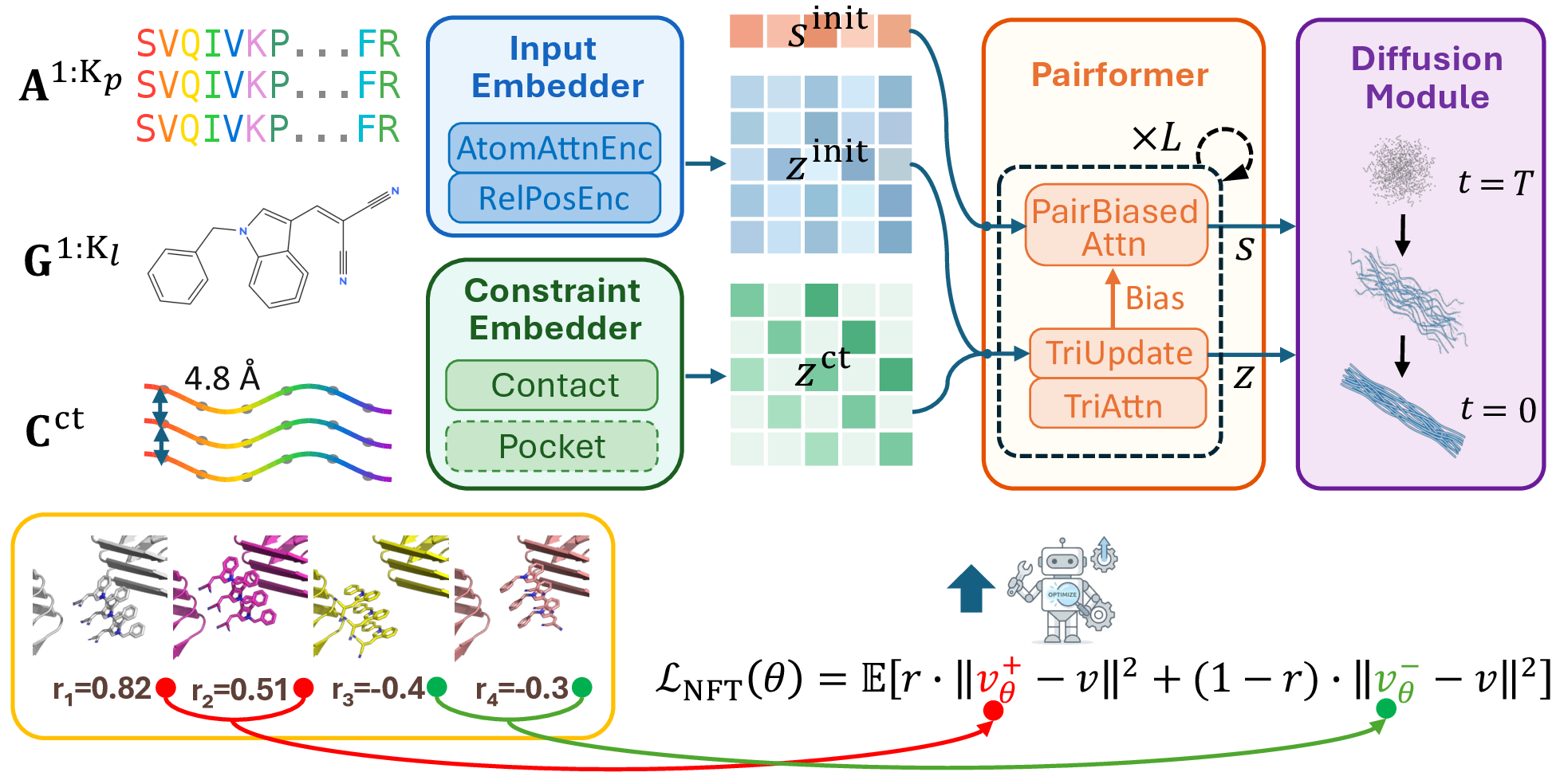
Our framework adopts a typical Pairformer–Diffusion architecture [3]. As shown in Figure 3, the input embedder produces initial single \((\mathbf{s}^{\text{init}})\) and pair \((\mathbf{z}^{\text{init}})\) representations, the Pairformer trunk refines them through triangle updates and pair-biased attention, and the diffusion module decodes atomic coordinates conditioned on the refined representations. We augment this pipeline with a ConstraintEmbedder that injects fibril-specific geometric priors into \(\mathbf{z}^{\text{init}}\).
3.2.0.1 Constraint-Aware Input Embedding.
A target fibril complex comprises \(K_p\) peptide chains that share an identical amino acid sequence and \(K_l\) ligand copies that share an identical molecular graph, which we denote by \(\mathbf{A}^{1:K_p}\) and \(\mathbf{G}^{1:K_l}\), respectively. These inputs are tokenised and embedded into initial per-token single representations \(\mathbf{s}_i^{\text{init}} \in \mathbb{R}^{c_s}\) and per-token-pair pair representations \(\mathbf{z}_{ij}^{\text{init}} \in \mathbb{R}^{c_z}\), where each token \(i\) corresponds to either a residue (for protein chains) or a heavy atom (for ligands). Here \(\mathbf{s}_i\) encodes the identity of token \(i\), while \(\mathbf{z}_{ij}\) encodes the pairwise relationship between tokens \(i\) and \(j\), including spatial proximity, bonding, and relative position.
To inject fibril-specific geometry into the pair representation, we introduce a ConstraintEmbedder that supports two types of constraints. The contact constraint \(\mathbf{C}^{\text{ct}}\) captures the translational periodicity of the fibril, i.e., the rigid-body shift of \({\sim}4.8\) Åbetween neighbouring chains along the fibril axis. It is realised as the \(\mathrm{C}_\alpha\)–\(\mathrm{C}_\alpha\) distance \(\mathbf{C}^{\text{ct}}_{ij} = \|\mathbf{r}_i - \mathbf{r}_j\|_2\) between residue tokens \(i\) and \(j\), where \(\mathbf{r}_i, \mathbf{r}_j \in \mathbb{R}^{3}\) are reference coordinates taken from the target fibril structure. The distance is then added to the pair representation through a linear projection: \[\mathbf{z}^{\text{init}}_{ij} \;\leftarrow\; \mathbf{z}^{\text{init}}_{ij} + \mathbf{W}_{\text{ct}}\,\mathbf{C}^{\text{ct}}_{ij}. \label{eq:constraint95embed}\tag{3}\] The pocket constraint \(\mathbf{C}^{\text{pkt}}\) marks the target binding region on the fibril surface, giving the ligand a spatial prior over where to bind; it is injected in the same manner via a separate projection \(\mathbf{W}_{\text{pkt}}\). All projections in the ConstraintEmbedder are zero-initialised, so that the added branch does not perturb the pair representation at initialization.
3.2.0.2 Pairformer Trunk and Diffusion Module.
The Pairformer trunk serves as the primary representation-learning engine of the model: it progressively refines \((\mathbf{s}^{\text{init}}, \mathbf{z}^{\text{init}})\) through \(L\) blocks that enforce triangle-inequality consistency on the pair track and propagate this geometry into the single track via pair-biased attention [3]. Because the constraints enter at \(\mathbf{z}^{\text{init}}\), they are carried through every Pairformer block and are ultimately encoded into the refined representations \((\mathbf{s}^{(L)}, \mathbf{z}^{(L)})\). The diffusion module then acts as a generative decoder: conditioned on \((\mathbf{s}^{(L)}, \mathbf{z}^{(L)})\), it parameterises the velocity field \(v_\theta(\mathbf{x}_t, t; \mathbf{s}^{(L)}, \mathbf{z}^{(L)})\) introduced in Eq. 1 , and at inference integrates it from \(t{=}1\) to \(t{=}0\) to denoise random coordinates into a plausible fibril–ligand complex \((\mathbf{x}_\text{prot}, \mathbf{x}_\text{lig})\).
3.3 Training↩︎
3.3.0.1 Data Curation.
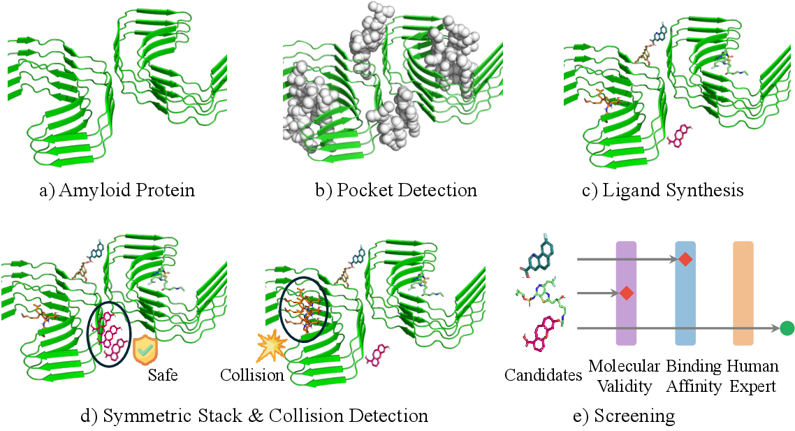
Because co-crystal structures of amyloid fibril–ligand complexes are exceedingly rare, we construct a synthetic training set through the pipeline illustrated in Figure 4. We first restrict the source pool to fibrils with a two-protofilament architecture and retain at least three consecutive chains per protofilament, so that both intra- and inter-protofilament binding interfaces are captured. For each fibril, candidate binding pockets along the cross-\(\beta\) grooves are identified with fpocket [54], and diverse small-molecule conformers are generated for each pocket using DrugFlow [11]. Each conformer is then replicated along the fibril axis according to the inter-chain translation, producing a symmetric stacking arrangement that mimics the cooperative binding mode observed in cryo-EM structures; arrangements with steric clashes or chemically unreasonable conformations are discarded by geometric filters. Three complementary judges evaluate the surviving poses in parallel: an LLM-based agent scoring molecular validity and pose plausibility, a docking scorer estimating protein–ligand binding affinity, and a human expert conducting final structural review; only poses passing all three are retained. This yields a curated dataset of fibril–ligand stacking poses suitable for supervised pre-training.
3.3.0.2 Warm-up Stage.
This stage warms up the model to the symmetric binding mode at a geometric level: how ligands intercalate into cross-\(\beta\) grooves, align along the fibril axis, and form periodically repeating stacking arrangements. We supervise the model on the subset of curated poses that passed the molecular-validity judge from the pipeline above, using a typical structure-prediction training objective [3] that combines three groups of losses: a flow-matching loss \(\mathcal{L}_\text{FM}\) that trains the diffusion module to denoise atomic coordinates towards the ground truth; a distogram loss \(\mathcal{L}_\text{dist}\) that supervises the trunk’s predicted distribution over pairwise residue distances; and three auxiliary confidence losses (\(\mathcal{L}_\text{pLDDT}\), \(\mathcal{L}_\text{PDE}\), \(\mathcal{L}_\text{PAE}\)) that supervise per-atom and per-pair error predictions. Following the classifier-free guidance strategy [55], the pocket constraint \(\mathbf{C}^{\text{pkt}}\) is dropped with \(50\%\) probability during training. This way, the network learns to generate both with and without the pocket prior, and we can combine the two at inference to modulate the strength of the prior.
3.3.0.3 Reinforcement Learning with Cooperative Binding Reward.
The warm-up stage captures the overall shape of symmetric stacking, but generated poses still deviate from realistic binding energetics. To close this gap, we fine-tune the warmed-up model \(v_\text{ref}\) with reinforcement learning [12] under a composite reward3 \[r(\mathbf{x}) \;=\; R_\text{bind}(\mathbf{x}) + \lambda\, R_\text{sym}(\mathbf{x}), \label{eq:reward}\tag{4}\] with two complementary terms. The binding energy combines the AutoDock Vina protein–ligand affinity \(\Delta G_\text{PL}\) [19], [20] with the MMFF94 [56] ligand–ligand stacking energy \(E_\text{stack}\) between the centre ligand and its symmetry-generated neighbours: \[R_\text{bind} \;=\; \Delta G_\text{PL} + R_\text{stack} \;\equiv\; \Delta G_{\mathrm{eff}}, \qquad R_\text{stack} = f \cdot E_\text{stack}, \label{eq:dg95eff}\tag{5}\] where \(f{=}0.005\) bridges gas-phase to solution-phase free energy [8]. The symmetry consistency \(R_\text{sym} = -\,\mathrm{RMSD}(\mathbf{T}\,\mathbf{x}_k,\, \mathbf{x}_{k+1})\) penalises deviations from the inter-chain rigid-body transformation \(\mathbf{T}\) (a \({\sim}4.8\) Åtranslation along the fibril axis) that should map ligand \(\mathbf{x}_k\) at chain \(k\) onto \(\mathbf{x}_{k+1}\) at chain \(k{+}1\). We minimise the RL objective \(\mathcal{L}_\text{NFT}(\theta)\) in Eq. 2 with this reward, adding a KL regulariser \(\beta_\text{KL}\|v_\theta - v_\text{ref}\|^2\) towards \(v_\text{ref}\) to stabilise training.
4 Experiments↩︎
4.1 Experimental Setup↩︎
4.1.0.1 Implementation.
The overall model architecture follows the typical Pairformer–Diffusion design [3]. Training follows the two-stage recipe described in §3.3. In the warm-up stage, we supervise the model on the subset of curated fibril–ligand stacking poses that pass the molecular-validity judge from our data-curation pipeline, with a learning rate of \(1\times 10^{-4}\). In the RL stage, the amyloid fibril–ligand complexes used as roll-out inputs are drawn from the amyloid ligand database of [5] (covering \(\alpha\)-synuclein, amyloid-\(\beta\), and tau fibril targets), filtered to entries with a two-protofilament architecture; we note that any ligand appearing in our evaluation sets is explicitly removed. A lower learning rate of \(3\times 10^{-6}\) is used for training stability. Both stages are trained on \(8\) NVIDIA A100 80G GPUs; the warm-up stage takes approximately \(3\) days and the RL stage approximately \(7\) days.4
4.1.0.2 Datasets.
We evaluate primarily on two complementary docking datasets. AmyDock-CryoEM draws ground-truth poses directly from PDB-deposited cryo-EM models; after filtering out solvent, buffer, and other non-specific small molecules, the set comprises 18 fibril–ligand complexes spanning tau, \(\alpha\)-synuclein, and related fibril-forming proteins. AmyDock-Synthetic generates reference poses through an agent-based sampling pipeline; after plausibility screening, binding-affinity scoring, and expert validation, the set comprises 57 fibril–ligand pairs that cover a broader range of ligand chemotypes than the cryo-EM structures alone. Additionally, to probe whether the predicted poses carry signal of the underlying binding energetics, we use a set of 47 small molecules with measured dissociation constants (\(K_d\)) against \(\alpha\)-synuclein fibrils published by [57]. This set has no ground-truth poses and is used solely for binding-affinity rank correlation; we refer to it as \(\alpha\)Syn-Bind.
4.1.0.3 Baselines.
We compare against seven docking methods spanning classical regression, diffusion, flow matching, and co-folding paradigms: DiffDock [1], DynamicBind [30], FABind [28], NeuralPLexer [2], FlowDock [31], Boltz-2 [58], and Chai-1 [34]. For a fair comparison, each baseline is also fine-tuned on AmyDock-Synthetic, as is our approach.
4.2 Evaluation↩︎
4.2.0.1 Quantitative Results.
On AmyDock-CryoEM and AmyDock-Synthetic, we measure docking accuracy with two metrics: Mean / Median RMSD, the heavy-atom RMSD between the best predicted pose and the ground truth (averaged or median across all pairs); and Hit rate (\(\leq 5\) Å), the fraction of pairs with RMSD \(\leq 5\) Å. On \(\alpha\)Syn-Bind, we measure binding-affinity correlation with Spearman \(\rho\) and its \(p\)-value between predicted binding scores and experimental \(\log(K_d/\mathrm{M})\). For baselines that only support single-ligand docking, we compare the predicted pose against the nearest ground-truth ligand copy.
| AmyDock-CryoEM | AmyDock-Synthetic | \(\alpha\)Syn-Bind | ||||||
|---|---|---|---|---|---|---|---|---|
| 2-4 (lr)5-7 (lr)8-9 Method | Mean \(\downarrow\) | Median \(\downarrow\) | Hit@5Å\(\uparrow\) | Mean \(\downarrow\) | Median \(\downarrow\) | Hit@5Å\(\uparrow\) | \(\rho\) \(\uparrow\) | \(p\) \(\downarrow\) |
| DiffDock | 17.67 | 13.68 | 0.0% | 19.19 | 19.68 | 3.5% | 0.191 | 0.197 |
| DynamicBind | 26.63 | 29.02 | 0.0% | 18.90 | 17.93 | 1.8% | 0.102 | 0.544 |
| FABind | 26.50 | 24.90 | 0.0% | 30.34 | 26.87 | 0.0% | 0.157 | 0.292 |
| NeuralPLexer | 17.43 | 19.00 | 5.6% | 19.78 | 16.56 | 0.0% | \(-\)0.291 | 0.047 |
| FlowDock | 19.95 | 21.52 | 0.0% | 20.69 | 19.88 | 0.0% | 0.148 | 0.322 |
| Boltz-2 | 28.27 | 28.67 | 0.0% | 37.13 | 33.87 | 0.0% | 0.223 | 0.132 |
| Chai-1 | 19.85 | 19.92 | 0.0% | 19.40 | 16.52 | 0.0% | \(-\)0.079 | 0.597 |
| (ours) | 8.70 | 4.89 | 50.0% | 7.35 | 3.84 | 68.4% | 0.419 | 0.004 |
4pt
As shown in Table 1, CORAL reaches a hit rate of \(\mathbf{68.4\%}\) at \(\leq 5\) Åon AmyDock-Synthetic (median RMSD \(\mathbf{3.84}\) Å) and \(\mathbf{50.0\%}\) on AmyDock-CryoEM, outperforming baselines whose single-ligand pocket formulations do not explicitly model the cooperative, periodic binding geometry of fibrils. On \(\alpha\)Syn-Bind, CORAL is the only method whose predicted binding scores correlate significantly (Spearman \(\rho{=}\mathbf{0.419}\), \(p{=}\mathbf{0.004}\)) with the experimental \(K_d\) values, indicating that the learned poses capture the underlying binding energetics rather than merely reproducing shape.
4.2.0.2 Qualitative Results.
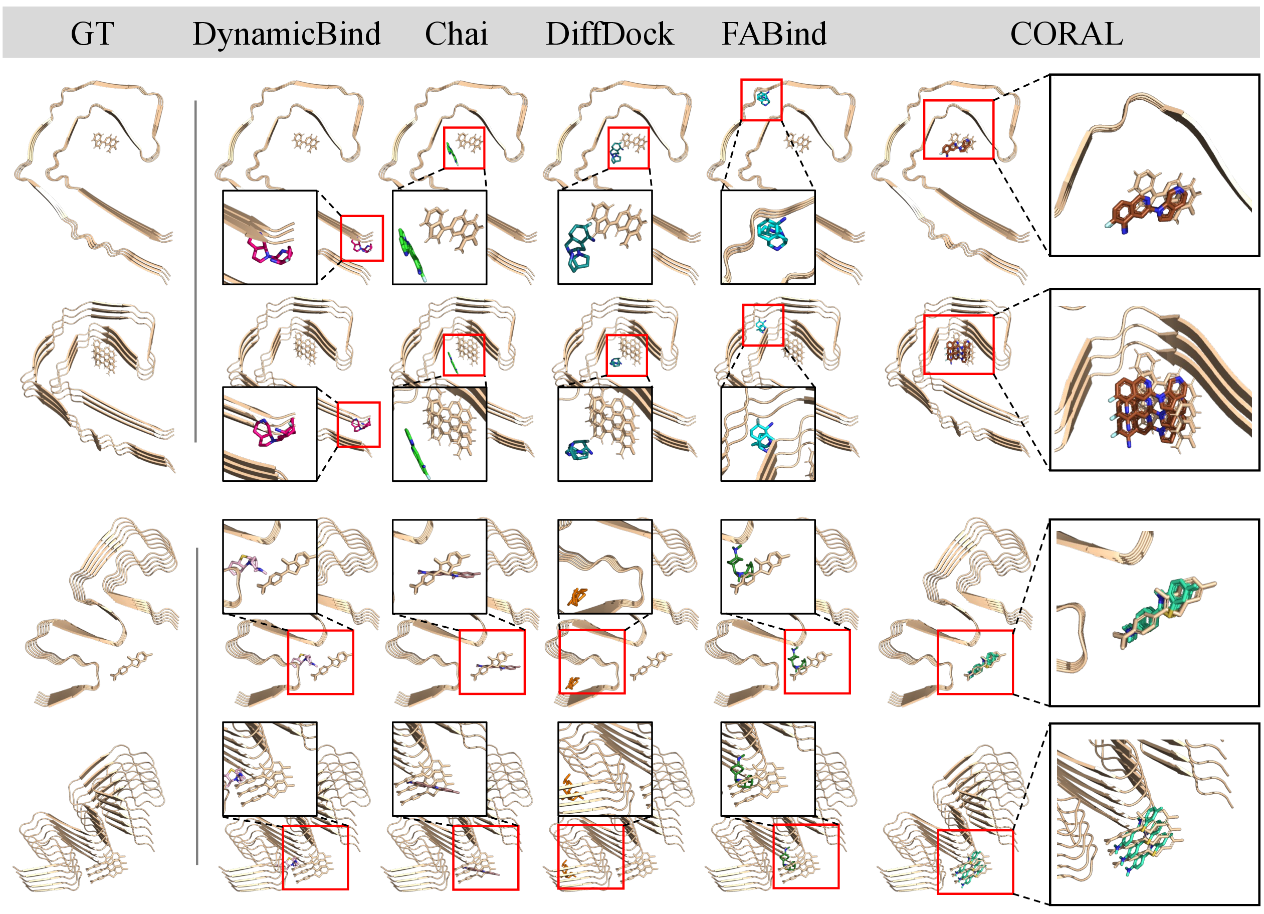
Figure 5 visualizes predictions on two representative AmyDock-CryoEM targets. Regression-based dockers such as FABind [28] collapse to a single averaged pose that drifts from the binding region, while the generative baselines dock each ligand independently and, lacking awareness of the fibril’s periodic geometry, tend to plaster the ligand vertically against the fibril surface or miss the intra-chain groove entirely—both failure modes yield large RMSD even when the per-ligand chemistry looks plausible. CORAL instead reproduces the periodic stacking of ligand copies across neighbouring peptide chains. The visual comparison corroborates the quantitative gap in Table 1 and indicates that learning the inter-ligand cooperative structure (not just single-pose protein–ligand fit) is the key driver of CORAL’s improvement.
4.3 Further Analysis↩︎
4.3.0.1 Ablation Study.
We ablate two key design choices of CORAL—the RL reward and the two-stage training recipe—on AmyDock-Synthetic (Table ¿tbl:tab:ablation?). Each variant modifies a single factor while keeping all other components identical to the full model. Removing \(R_\text{stack}\) collapses \(R_\text{bind}\) to plain protein–ligand affinity, eliminating the cooperative inter-ligand signal and degrading \(\Delta G_{\mathrm{eff}}\); removing \(R_\text{sym}\) has a milder effect on RMSD because the warm-up stage has already established much of the stacking geometry, so \(R_\text{sym}\) mainly serves as a fine-tuning anchor during RL; removing the KL term destabilises training and the model diverges from the warmed-up shape prior. Finally, RL without warm-up converges to a worse local optimum—without a shape prior to start from, the policy explores from scratch and lands on noisier stacking geometry—while warm-up without RL produces plausible stacking but under-performs energetically; only the combined recipe achieves both accurate geometry and favourable binding energetics.
4pt
@lcccc Variant & Mean RMSD \(\downarrow\) & Median RMSD \(\downarrow\) & Mean \(\Delta G_{\mathrm{eff}}\) \(\downarrow\) & Median \(\Delta G_{\mathrm{eff}}\) \(\downarrow\)
(full) & 7.35 & 3.84 & -2.24 & -2.44
\(-\,R_\text{sym}\) (no symmetry term) & 7.92 & 4.31 & -2.07 & -2.21
\(-\,R_\text{stack}\) (no cooperative term) & 8.21 & 4.46 & -0.78 & -0.95
\(-\,\)KL (no stability regulariser) & 12.07 & 8.13 & -1.32 & -1.45
Warm-up only (no RL) & 8.67 & 5.18 & -1.41 & -1.58
RL only (no warm-up) & 13.45 & 9.27 & -0.72 & -0.88
4.3.0.2 Case Study.
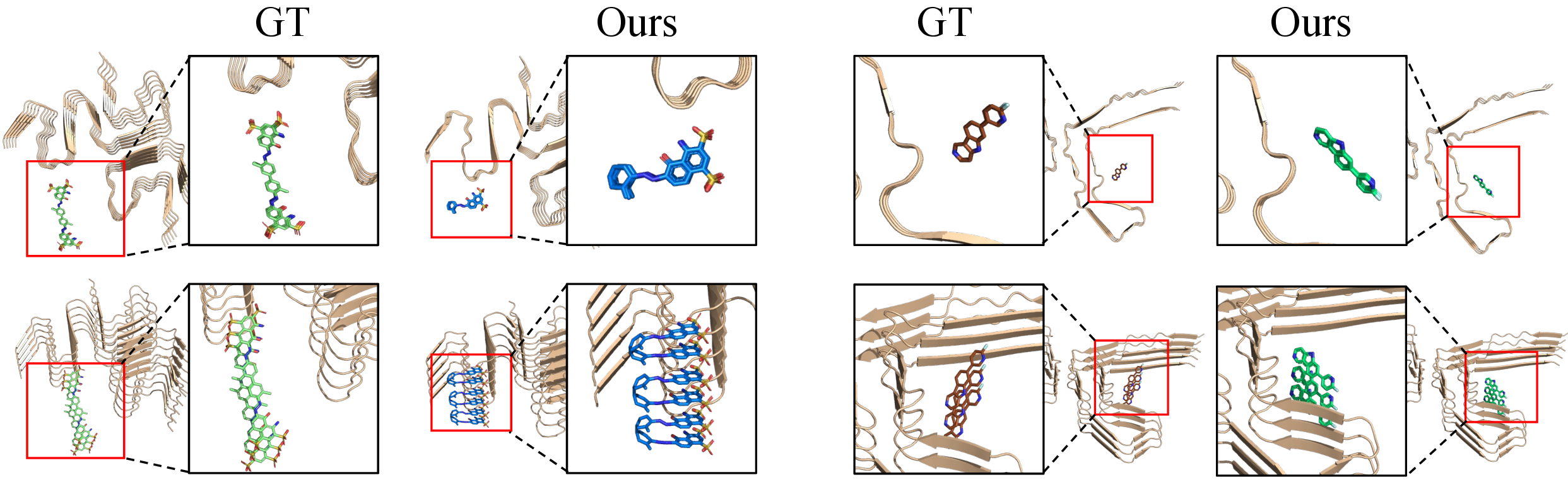
We highlight a few cases where CORAL underperforms (Figure 6). First, the model folds the ligand back on itself so that one segment stacks with neighbouring copies while the other bends toward the protein surface (Figure 6, left), letting a single pose gain both stacking and protein-contact energy at once. Second, the model places the ligand at the correct binding site but rotates it sideways from the canonical axial orientation to enlarge protein contact (Figure 6, right).
5 Conclusion↩︎
We present CORAL, the first deep learning-based docking framework tailored to amyloid fibril–ligand complexes. Our framework tackles cooperative multi-ligand docking on amyloid fibrils—a binding mode that single-pocket docking models are not designed to capture: it injects fibril-periodicity priors into the structure model and refines pose distributions through online reinforcement learning under a stacking-aware reward, sidestepping the scarcity of fibril–ligand co-crystal supervision. Across all three evaluation datasets, our framework substantially outperforms existing docking methods and uniquely produces scores that correlate with experimental binding affinities.
Limitations and Broader Impact. Our evaluation covers fibrils associated with three major neurodegenerative diseases (tau, \(\alpha\)-synuclein, amyloid-\(\beta\)); extending to transthyretin, light-chain, and other amyloid aggregates is a natural next step, and we plan to integrate de novo ligand generation, our docking framework, and downstream filtering into a single agent-orchestrated closed-loop pipeline [59], [60] for automated discovery of fibril-binding candidates with minimal human intervention. The framework aims to accelerate early-stage drug discovery for Alzheimer’s, Parkinson’s, and related neurodegenerative diseases; it predicts binding geometries rather than generating novel bioactive compounds, posing no direct dual-use concern, while predicted poses still require experimental validation before any downstream use.
The research reported in this publication was supported by a gift from Google, administered through the King Abdullah University of Science and Technology (KAUST) – Center of Excellence for Generative AI under award number 5940.
Appendix
This appendix provides additional details supporting the main paper. §6 describes the architecture, supervised warm-up, the synthetic data-curation pipeline used to construct AmyDock-Synthetic, and the AmyDock benchmark. §7 presents the full reinforcement-learning algorithm, the cooperative binding reward design, and its underlying physics. §8 provides additional qualitative visualisations of CORAL’s predicted fibril–ligand poses.
6 Warm-up and Data Curation↩︎
This section provides additional details on the warm-up training stage and the synthetic data-curation pipeline used to construct AmyDock-Synthetic. Because amyloid fibril–ligand co-crystal structures are scarce, we curate a synthetic dataset of symmetric stacking poses via an agent-driven pipeline (§[app:data95curation]), and warm up the model on this dataset to first establish the symmetric binding mode at a geometric level (§6.1) before reinforcement-learning fine-tuning toward cooperative binding energetics (Appendix 7).
6.1 Training Objective↩︎
For the warm-up stage, we adopt the standard AlphaFold-3-style structure-prediction objective [3], [61], which combines three groups of losses: (i) a diffusion loss \(\mathcal{L}_\text{diff}\) that supervises atomic coordinates (instantiating \(\mathcal{L}_\text{FM}\) in Eq. 1 ), (ii) a distogram loss \(\mathcal{L}_\text{dist}\) that supervises pairwise residue distances, and (iii) a confidence loss \(\mathcal{L}_\text{conf}\) that trains the model to predict its own per-atom and per-pair errors. The total warm-up objective is \[\mathcal{L}_\text{SFT} \;=\; \alpha_\text{diff}\,\mathcal{L}_\text{diff} \;+\; \alpha_\text{dist}\,\mathcal{L}_\text{dist} \;+\; \alpha_\text{conf}\,\mathcal{L}_\text{conf}, \label{eq:sft95total95loss}\tag{6}\] with each component defined as \[\begin{align} \mathcal{L}_\text{diff} &= \mathcal{L}_\text{MSE} + \alpha_\text{bond}\,\mathcal{L}_\text{bond} + w_\text{lddt}\,\mathcal{L}_\text{smooth-LDDT}, \tag{7} \\ \mathcal{L}_\text{conf} &= \mathcal{L}_\text{pLDDT} + \mathcal{L}_\text{PDE} + \alpha_\text{pae}\,\mathcal{L}_\text{PAE}. \tag{8} \end{align}\] Here \(\mathcal{L}_\text{MSE}\) is the weighted per-atom coordinate MSE (with element-specific weights \(w_\text{protein}{=}1\), \(w_\text{DNA}{=}w_\text{RNA}{=}5\), \(w_\text{ligand}{=}10\)), \(\mathcal{L}_\text{bond}\) is a bond-length consistency loss, \(\mathcal{L}_\text{smooth-LDDT}\) is the smooth-LDDT loss, \(\mathcal{L}_\text{dist}\) is the distogram cross-entropy over binned \(\text{C}_\beta\)–\(\text{C}_\beta\) distances, and \(\mathcal{L}_\text{pLDDT}, \mathcal{L}_\text{PDE}, \mathcal{L}_\text{PAE}\) are the three confidence-head classification losses. The global weights are empirically set as \(\alpha_\text{diff}{=}4.0\), \(\alpha_\text{dist}{=}0.03\), \(\alpha_\text{conf}{=}10^{-4}\), \(w_\text{lddt}{=}1.0\), while \(\alpha_\text{bond}\) and \(\alpha_\text{pae}\) act as switches that are set to \(0\) during early training and turned on (\(=1\)) in the final fine-tuning stage.
6.1.0.1 Generic Docking Pre-Training.
Before amyloid-specific warm-up, we run a generic docking pre-training stage on a large, diverse collection of protein–ligand co-crystals using the objective in Eq. 6 . The training corpus aggregates four established protein–ligand datasets: PLINDER [62], Binding MOAD [63], HiQBind [64], and SPINDR [65]. The goal is to expose the diffusion module to a broad range of small-molecule geometries and chemotypes, providing a strong starting checkpoint for the subsequent amyloid-specific fine-tuning.
6.1.0.2 Geometry Constraint.
Beyond the loss design, we inject two fibril-specific priors into the pair representation \(\mathbf{z}^{\text{init}}\) via the ConstraintEmbedder (§3.2). The contact constraint \(\mathbf{C}^{\text{ct}}\) encodes the translational periodicity of cross-\(\beta\) amyloid fibrils, which are stacks of identical \(\beta\)-strand layers separated by a characteristic inter-strand C\(_\alpha\)–C\(_\alpha\) spacing of \({\sim}4.8\) Å. For each pair of residue tokens \((i, j)\) we compute the pairwise distance \(\mathbf{C}^{\text{ct}}_{ij} = \|\mathbf{r}_i - \mathbf{r}_j\|_2\) from the reference fibril structure and inject it through a learned linear projection \(\mathbf{W}_{\text{ct}}\) (Eq. 3 ); the constraint then propagates to every Pairformer block, biasing attention toward the periodic ladder of inter-chain contacts characteristic of cross-\(\beta\) assemblies. The pocket constraint \(\mathbf{C}^{\text{pkt}}\) marks the candidate binding region on the fibril surface (the residues bordering a cross-\(\beta\) groove), providing a soft spatial prior over where ligands should bind. It is injected with the same mechanism through a separate projection \(\mathbf{W}_{\text{pkt}}\). Both projections are zero-initialised so that the constraint branch does not perturb the pair representation at the start of training. Following classifier-free guidance [55], \(\mathbf{C}^{\text{pkt}}\) is dropped with probability \(0.5\) during warm-up; the model thus learns both with and without the pocket prior, and the prior strength can be modulated at inference by interpolating between the conditional and unconditional velocity fields.
6.2 Data Curation↩︎
Resolved co-crystal structures of amyloid fibril–ligand complexes are exceptionally scarce: even with recent cryo-EM advances, only a handful have been structurally characterised, making supervised training of fibril-specific docking models infeasible from experimental data alone. To overcome this bottleneck, we synthesise plausible cooperative stacking poses through an agent-driven pipeline (Figure 7) and validate them via geometric, LLM-based, and expert checks, yielding the AmyDock-Synthetic training set used in the warm-up stage. The remainder of this subsection describes each stage in detail.
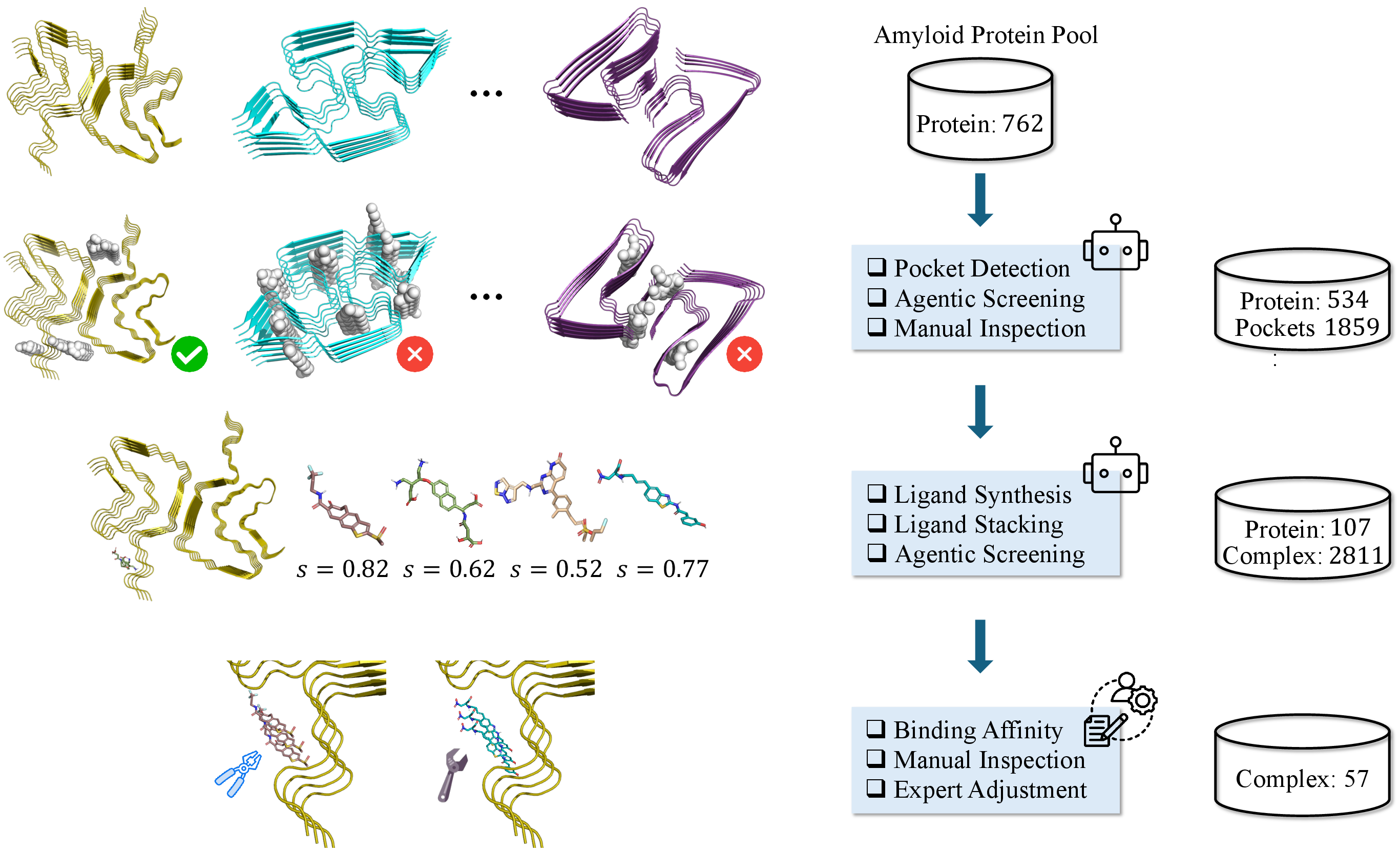
6.2.0.1 Curation Workflow.
The workflow comprises four sequential stages: (1) pocket detection on each fibril surface; (2) conformer generation at every detected pocket; (3) symmetric axial replication with collision filtering to mimic cooperative stacking; and (4) agentic and chemical screening to retain only chemically valid, plausibly binding poses. We report intermediate counts at each stage below.
Pocket detection. We identify candidate binding sites on the fibril surface using two complementary tools, Fpocket [54] and CaverDock [66], and merge their outputs followed by manual expert inspection to discard non-physical or duplicate sites. This yields 1,859 candidate pockets across all fibril targets.
Conformer generation. For each pocket, we generate 100 candidate ligands using a fine-tuned variant of DrugFlow [11]; we fine-tune DrugFlow on training targets that contain \(\beta\)-sheet structures, biasing the generative distribution toward chemotypes more compatible with cross-\(\beta\) groove binding. This stage takes approximately one week on 4 NVIDIA A100 GPUs.
Symmetric stacking and collision filtering. Each conformer is replicated along the fibril axis and tested for inter-ligand and ligand–protein steric clashes (atom-pair distance \(<2.0\) Å). After this filter, 8,166 candidate stacking arrangements remain.
Agentic and chemical screening. Surviving candidates are screened by an LLM-based agent (prompts in §6.2.0.2) for binding-mode plausibility, and validated for chemical correctness with RDKit’s sanitisation routines. The final AmyDock-Synthetic warm-up training set contains approximately 2,000 poses.
6.2.0.2 LLM-Based Pose Screening Prompts.
During data curation, candidate stacking poses produced by DrugFlow and axial replication are filtered by an LLM agent that judges whether a small molecule is properly docked in a fibril groove/channel. The agent receives a PDB snippet of the fibril–ligand complex and outputs a binary verdict together with a continuous confidence score in \([0, 1]\). We use the following prompts with GPT-5.
You are an expert structural biologist and computational chemist specializing in amyloid fibril structures and small molecule binding. Your task is to evaluate whether a small molecule is properly docked in the grooves/channels of a fibril protein structure. Fibril proteins have characteristic cross-\(\beta\) sheet structures with grooves or channels running along the fibril axis where small molecules can bind.
Key characteristics of proper fibril groove docking:
(1) Location: the molecule should be positioned in the groove/channel between protein chains, not on the surface or outside the fibril.
(2) Orientation: the molecule should align along the fibril axis, not perpendicular to it.
(3) Interactions: favorable contacts with groove walls, including Van der Waals contacts (3.0–5.0 Å), hydrogen bonds (2.5–3.5 Å), \(\pi\)-\(\pi\) stacking (3.3–4.5 Å) where applicable, and
hydrophobic contacts.
(4) Shape complementarity: the molecule should fit well into the groove geometry.
(5) No clashes: no severe steric clashes (\(<\)2.0 Å).
I have a PDB structure file containing a fibril protein with a docked small molecule. Please evaluate whether the small molecule is properly docked in the fibril groove/channel.
PDB File Content: {pdb_content}
Evaluation Criteria:
(1) Location: is the molecule positioned in a groove/channel between protein chains (not on surface)?
(2) Orientation: is the molecule aligned along the fibril axis?
(3) Interactions: does the molecule form favorable interactions with groove residues (VdW, H-bond, \(\pi\)-\(\pi\), hydrophobic)?
(4) Shape complementarity: does the molecule fit well into the groove geometry?
(5) No clashes: no severe steric clashes (\(<\)2.0 Å).
Output Format:
Answer: [Yes or No]
Score: [number between 0.0 and 1.0]
A pose is retained if Answer = Yes and Score\(\geq\)0.5.
6.2.0.3 AmyDock Benchmark.
After the LLM and chemistry filters, surviving stacking poses are inspected by domain experts who additionally adjust ambiguous cases, producing the final AmyDock-Synthetic set used for warm-up training. Both AmyDock-Synthetic and the experimentally-resolved AmyDock-CryoEM evaluation set consist of two-protofilament fibrils with at least three consecutive chains per protofilament, covering both intra- and inter-protofilament binding interfaces; the per-fibril composition (tau, \(\alpha\)-synuclein, related), ligand chemotype distribution, and PDB indices for AmyDock-CryoEM will be released alongside the dataset.
7 Reinforcement Learning with Cooperative Reward↩︎
This section details the reinforcement-learning stage of CORALused in §3.3. We first present the training objective based on DiffusionNFT [12] (§7.1), then expand the composite cooperative-binding reward into its constituent terms and derive the gas-to-solution-phase scaling factor that bridges the MMFF94 stacking energy to the protein–ligand affinity (§7.2).
7.1 Training Objective↩︎
DiffusionNFT [12] is an online reinforcement-learning algorithm for diffusion (and flow-matching) models that operates directly on the forward process and avoids explicit likelihood estimation.
7.1.0.1 Forward Process and Sampling.
Given a clean sample \(\mathbf{x}_0 \sim p_{\text{data}}\) and a noise sample \(\boldsymbol{\epsilon} \sim \mathcal{N}(\mathbf{0}, \mathbf{I})\), the forward process interpolates between data and noise according to a schedule \((\alpha_t, \sigma_t)\): \[\mathbf{x}_t \;=\; \alpha_t \mathbf{x}_0 + \sigma_t \boldsymbol{\epsilon}, \qquad t \in [0, 1],\] with target velocity \[\mathbf{v}(\mathbf{x}_t, t) \;=\; \dot{\alpha}_t \mathbf{x}_0 + \dot{\sigma}_t \boldsymbol{\epsilon}. \label{eq:fm95target}\tag{9}\] Standard flow matching trains a velocity field \(v_\theta\) by \(\mathcal{L}_\text{FM}(\theta) = \mathbb{E}\,\|v_\theta(\mathbf{x}_t, t) - \mathbf{v}\|_2^2\). At inference, samples are generated by integrating the learned velocity field along the reverse direction: starting from \(\mathbf{x}_1 \sim \mathcal{N}(\mathbf{0}, \mathbf{I})\) and solving \(\mathrm{d}\mathbf{x}_t / \mathrm{d}t = v_\theta(\mathbf{x}_t, t)\) from \(t=1\) to \(t=0\) to obtain a clean sample \(\mathbf{x}_0\).
7.1.0.2 Implicit Positive / Negative Policies.
Given a frozen sampling policy \(v_\text{old}\) and the current policy \(v_\theta\), DiffusionNFT defines two implicit velocity fields through reparameterisation: \[\begin{align} v_\theta^{+}(\mathbf{x}_t, t) &:= (1 - \beta)\,v_\text{old}(\mathbf{x}_t, t) + \beta\,v_\theta(\mathbf{x}_t, t), \tag{10}\\ v_\theta^{-}(\mathbf{x}_t, t) &:= (1 + \beta)\,v_\text{old}(\mathbf{x}_t, t) - \beta\,v_\theta(\mathbf{x}_t, t), \tag{11} \end{align}\] where \(\beta \in (0, 1)\) is a mixing coefficient. Here \(v_\theta^{+}\) is the positive policy (interpolating from \(v_\text{old}\) towards \(v_\theta\)) and \(v_\theta^{-}\) is the negative policy (extrapolating away from \(v_\theta\)); both are fully determined by \(v_\theta\), with no auxiliary guidance networks.
7.1.0.3 Reward-Weighted Loss.
Let \(r(\mathbf{x}_0) \in [0, 1]\) denote the scalar optimality probability of a sampled clean trajectory endpoint \(\mathbf{x}_0\) (we describe how we obtain \(r\) from our composite reward in the next subsection). The NFT loss minimised at each optimisation step is \[\mathcal{L}_\text{NFT}(\theta) \;=\; \mathbb{E}\!\left[\, r(\mathbf{x}_0)\,\|v_\theta^{+}(\mathbf{x}_t, t) - \mathbf{v}\|_2^2 \;+\; (1 - r(\mathbf{x}_0))\,\|v_\theta^{-}(\mathbf{x}_t, t) - \mathbf{v}\|_2^2 \,\right], \label{eq:nft95loss95full}\tag{12}\] with the expectation taken over \((\mathbf{x}_0, \boldsymbol{\epsilon}, t)\). High-reward samples are regressed by the positive branch \(v_\theta^{+}\) and low-reward samples by the negative branch \(v_\theta^{-}\), so the policy is simultaneously pushed towards \(v_\theta^{+}\) and away from \(v_\theta^{-}\). We refer to [12] for the gradient analysis showing this corresponds to a soft importance-weighted policy improvement without explicit likelihood ratios.
7.1.0.4 Reward Normalisation.
Our composite reward \(r(\mathbf{x}) = R_\text{bind}(\mathbf{x}) + \lambda\,R_\text{sym}(\mathbf{x})\) (Eq. 4 ) is a real-valued score, not a probability. Following the original paper, we convert it to \(r \in [0, 1]\) by group-relative normalisation within each group of \(G\) on-policy rollouts \(\{\mathbf{x}^{(i)}\}_{i=1}^{G}\) sampled from the same complex: \[\tilde{r}^{(i)} \;=\; \frac{r(\mathbf{x}^{(i)}) - \min_j r(\mathbf{x}^{(j)})}{\max_j r(\mathbf{x}^{(j)}) - \min_j r(\mathbf{x}^{(j)}) + \varepsilon}, \label{eq:reward95norm}\tag{13}\] so that within each batch the best rollout receives \(\tilde{r} \approx 1\) (regressed by \(v_\theta^{+}\)) and the worst receives \(\tilde{r} \approx 0\) (regressed by \(v_\theta^{-}\)). The small constant \(\varepsilon = 10^{-6}\) prevents division by zero when all rewards are equal.
7.1.0.5 Sampling Policy Update.
To keep the on-policy assumption approximately valid while preventing \(v_\text{old}\) from lagging too far behind \(v_\theta\), we update \(v_\text{old}\) by a soft exponential moving average (EMA) after every \(N_\text{upd}\) gradient steps: \[\theta_\text{old} \;\leftarrow\; \eta\,\theta_\text{old} + (1 - \eta)\,\theta, \label{eq:ema}\tag{14}\] with \(\eta \in [0, 1]\) the EMA coefficient.
7.1.0.6 KL Regularisation.
To prevent the policy from drifting away from the warmed-up shape prior during RL—without which the ligand pose tends to break symmetric stacking in early iterations, yielding noisier reward signals and slower convergence—we add a KL-style regulariser towards the frozen warmed-up reference \(v_\text{ref}\) (obtained at the end of the warm-up stage, before RL starts): \[\mathcal{L}_\text{KL}(\theta) \;=\; \mathbb{E}_{\mathbf{x}_t, t}\!\left[\, \|v_\theta(\mathbf{x}_t, t) - v_\text{ref}(\mathbf{x}_t, t)\|_2^2 \,\right],\] and optimise the combined objective \(\mathcal{L}_\text{NFT}(\theta) + \beta_\text{KL}\,\mathcal{L}_\text{KL}(\theta)\). We treat this as a proximal trust region around \(v_\text{ref}\) rather than a strict KL divergence (which would be expensive to estimate for a diffusion policy).
7.1.0.7 Hyperparameters.
The mixing coefficient \(\beta\), EMA coefficient \(\eta\), and group size \(G\) follow the defaults of DiffusionNFT [12]. We update \(v_\text{old}\) every \(N_\text{upd}{=}8\) epochs (rather than every step) to give the behaviour policy a more stable optimisation window on our relatively small cooperative-binding training set, and increase the KL weight from the DiffusionNFT default of \(10^{-3}\) to \(\beta_\text{KL}{=}10^{-2}\) to constrain policy drift from the warmed-up reference. The symmetry-reward weight \(\lambda\) was tuned on a held-out subset of fibrils.
| Symbol | Value | Description |
|---|---|---|
| \(\beta\) | \(0.1\) | Mixing coefficient in \(v_\theta^{\pm}\) (Eq. [eq:nft95vplus]–[eq:nft95vminus]) |
| \(\lambda\) | \(0.01\) | Weight of \(R_\text{sym}\) in the composite reward |
| \(\beta_\text{KL}\) | \(0.01\) | KL regularisation weight |
| \(\eta\) | \(0.5\) | EMA coefficient for \(v_\text{old}\) (Eq. [eq:ema]) |
| \(N_\text{upd}\) | \(8\) | Gradient steps between \(v_\text{old}\) updates |
| \(G\) | \(24\) | Rollouts per complex for reward normalisation (Eq. [eq:reward95norm]) |
7.2 Reward Design↩︎
We now unpack the composite reward \(r(\mathbf{x}) = R_\text{bind}(\mathbf{x}) + \lambda\, R_\text{sym}(\mathbf{x})\) from §3.3. The binding term \(R_\text{bind}\) couples a thermodynamic protein–ligand affinity with a cooperative ligand–ligand stacking energy; the symmetry term \(R_\text{sym}\) enforces consistency between neighbouring binding sites. The remainder of this section defines each term and derives the gas-to-solution-phase scaling factor \(f\) inside \(R_\text{bind}\) from a cooperative-binding model; \(f\) itself is set from physics rather than fit to data.
7.2.0.1 Binding Energy.
Small-molecule ligands that bind amyloid fibrils occupy periodic binding sites along the cross-\(\beta\) groove, where adjacent ligands are separated by the inter-strand distance (\({\sim}4.7\)–\(4.9\) Å). This periodic arrangement gives rise to cooperative ligand–ligand interactions that are not captured by standard protein–ligand docking scores [7], [8]. We therefore augment the AutoDock Vina protein–ligand affinity with a stacking-energy correction: \[R_\text{bind} \;=\; \Delta G_\text{PL} + f \cdot E_\text{stack}, \label{eq:rbind95app}\tag{15}\] where \(\Delta G_\text{PL}\) is the Vina affinity (kcal/mol) [19], [20], calibrated against experimental binding free energies in aqueous solution, and \(E_\text{stack}\) is the ligand–ligand intermolecular energy computed with the MMFF94 force field [56] between the centre ligand and its symmetry-generated neighbouring copies. The two terms are not natively on the same thermodynamic scale: \(\Delta G_\text{PL}\) already reflects solution-phase binding (where solvation and entropy are felt), whereas \(E_\text{stack}\) is a vacuum pairwise interaction that omits the desolvation and entropic costs incurred when two ligands stack in water and is therefore typically one to two orders of magnitude larger in magnitude. The factor \(f\) is a thermodynamic attenuation that brings \(E_\text{stack}\) onto the same solution-phase scale as \(\Delta G_\text{PL}\) [8]; we set \(f = 0.005\), with the physical derivation given below.
7.2.0.2 Physical Basis for the Scaling Factor.
The quantity we actually need is the per-pair solution-phase cooperative free energy \(C_L\)—how much one occupied neighbour contributes to a ligand’s binding free energy in water. Smith et al. [8] showed via an Ising lattice-gas analysis that, for ligands binding along a fibril groove, the observed cooperative shift in apparent affinity is captured by a single pairwise \(C_L\), justifying our use of one attenuation factor \(f\) rather than a many-body correction. To relate \(C_L\) to the vacuum quantity \(E_\text{stack}\) that we can actually compute, we apply the standard binding-energy decomposition of Gilson and Zhou [67]: \[C_L \;=\; E_{\mathrm{stack}}^{\mathrm{gas}} + \Delta G_{\mathrm{desolv}} + T\Delta S_{\mathrm{restrict}}, \label{eq:cl95decomp}\tag{16}\] where \(E_\text{stack}^\text{gas}\) is the favourable vacuum pairwise interaction (what MMFF94 returns), \(\Delta G_{\mathrm{desolv}}\) is the desolvation penalty incurred when adjacent ligands bury their contact surfaces upon stacking, and \(T\Delta S_{\mathrm{restrict}}\) is the entropic cost of restricting translational and rotational freedom relative to independent binding. The first term is large and favourable (\(|E_\text{stack}^\text{gas}| \sim 50\)–\(300\) kcal/mol for drug-like molecules) but is opposed by the latter two; for stacking in a fibril groove these opposing contributions cancel \(99\)–\(99.5\%\) of the gas-phase interaction [67], leaving \(C_L \approx f \cdot E_\text{stack}\) with \(f \approx 0.005\).
7.2.0.3 MMFF94 Energy Computation.
Having justified the value of \(f\), we now specify how the gas-phase \(E_\text{stack}\) itself is computed in practice. We take the pairwise atomic sum \(E_\text{stack} = \sum_{i \in A} \sum_{j \in B} \left[ E_\text{VdW}(r_{ij}) + E_\text{Coul}(r_{ij}) \right]\), where \(A\) and \(B\) denote the atom sets of the centre ligand and a neighbouring ligand copy, respectively. The van der Waals term uses the Halgren Buffered 14-7 potential [56]: \[E_\text{VdW}(r) = \varepsilon_{ij} \left(\frac{1.07}{\rho + 0.07}\right)^{\!7} \left(\frac{1.12}{\rho^7 + 0.12} - 2\right), \label{eq:buffered147}\tag{17}\] with \(\rho = r/R^*_{ij}\), \(\varepsilon_{ij} = \sqrt{\varepsilon_i \varepsilon_j}\), and \(R^*_{ij} = R^*_i + R^*_j\) from the MMFF94 force field [56]. The Coulomb term is \(E_\text{Coul}(r) = 332.07\, q_i q_j / (r + 0.05)\), where \(q_i, q_j\) are MMFF94 partial charges and the \(0.05\) Åbuffer prevents singularities at short distances. A pairwise cutoff of \(12\) Åis applied.
7.2.0.4 Symmetry Consistency.
The second reward term enforces that ligand poses at neighbouring sites are related by the same rigid-body operation that governs the protein repeat units. Let \(\mathbf{T} = (\mathbf{R}, \mathbf{t})\) denote the inter-chain transformation that maps chain \(k\) to chain \(k{+}1\) (a rigid-body translation of \({\sim}4.8\) Åalong the fibril axis); we obtain \(\mathbf{T}\) by Kabsch alignment [68] of the C\(_\alpha\) atoms of chain \(k\) onto those of its nearest neighbour chain \(k{+}1\) within the same protofilament, with the SVD-based closed-form solution and a reflection-correcting sign on the determinant. Denoting by \(\mathbf{x}_k\) the ligand pose bound to the \(k\)-th peptide chain, the transformed pose \(\mathbf{T}\,\mathbf{x}_k\) should coincide with \(\mathbf{x}_{k+1}\), the ligand bound to the neighbouring chain, motivating: \[R_\text{sym} \;=\; -\,\mathrm{RMSD}\!\left(\mathbf{T}\,\mathbf{x}_k,\; \mathbf{x}_{k+1}\right).\]
7.2.0.5 Training Dynamics.
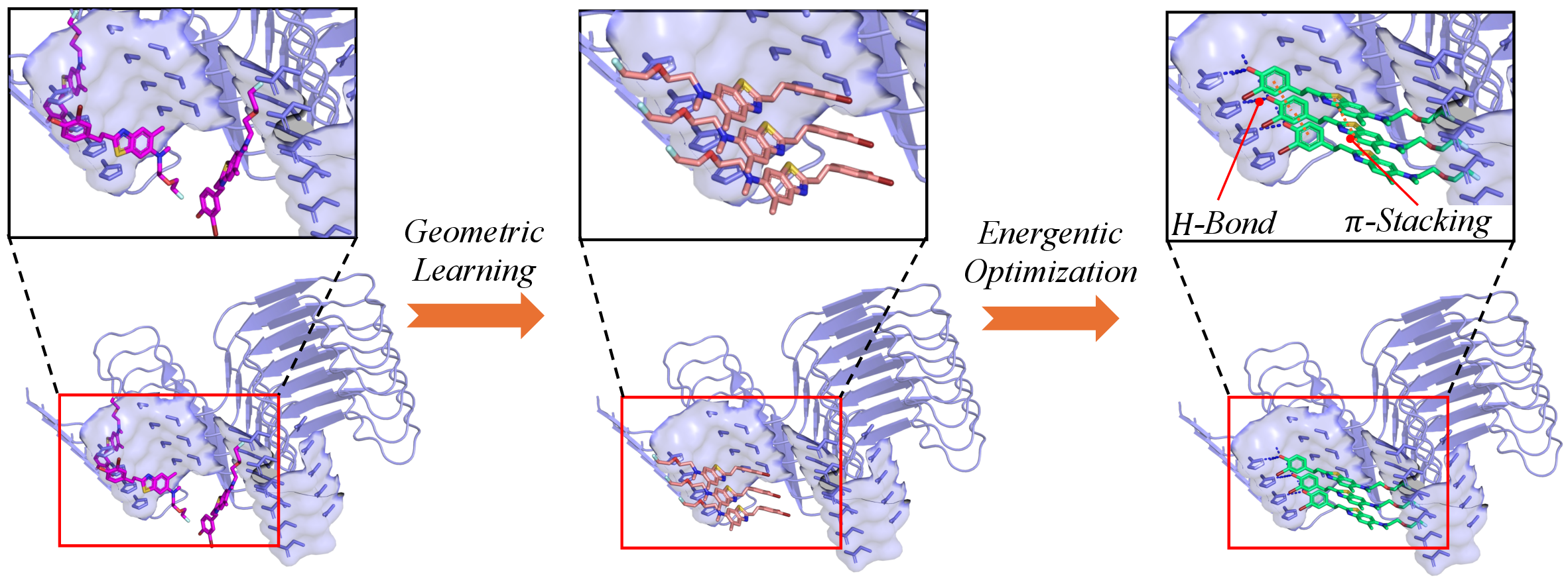
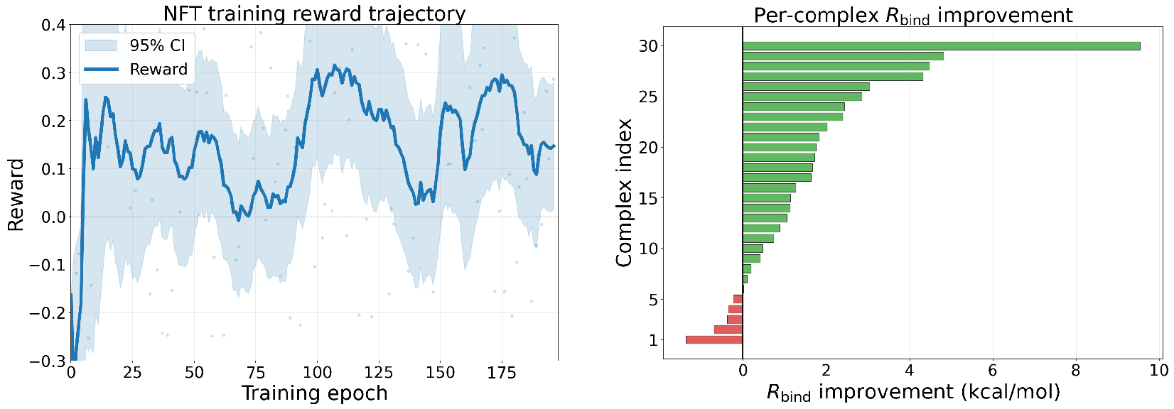
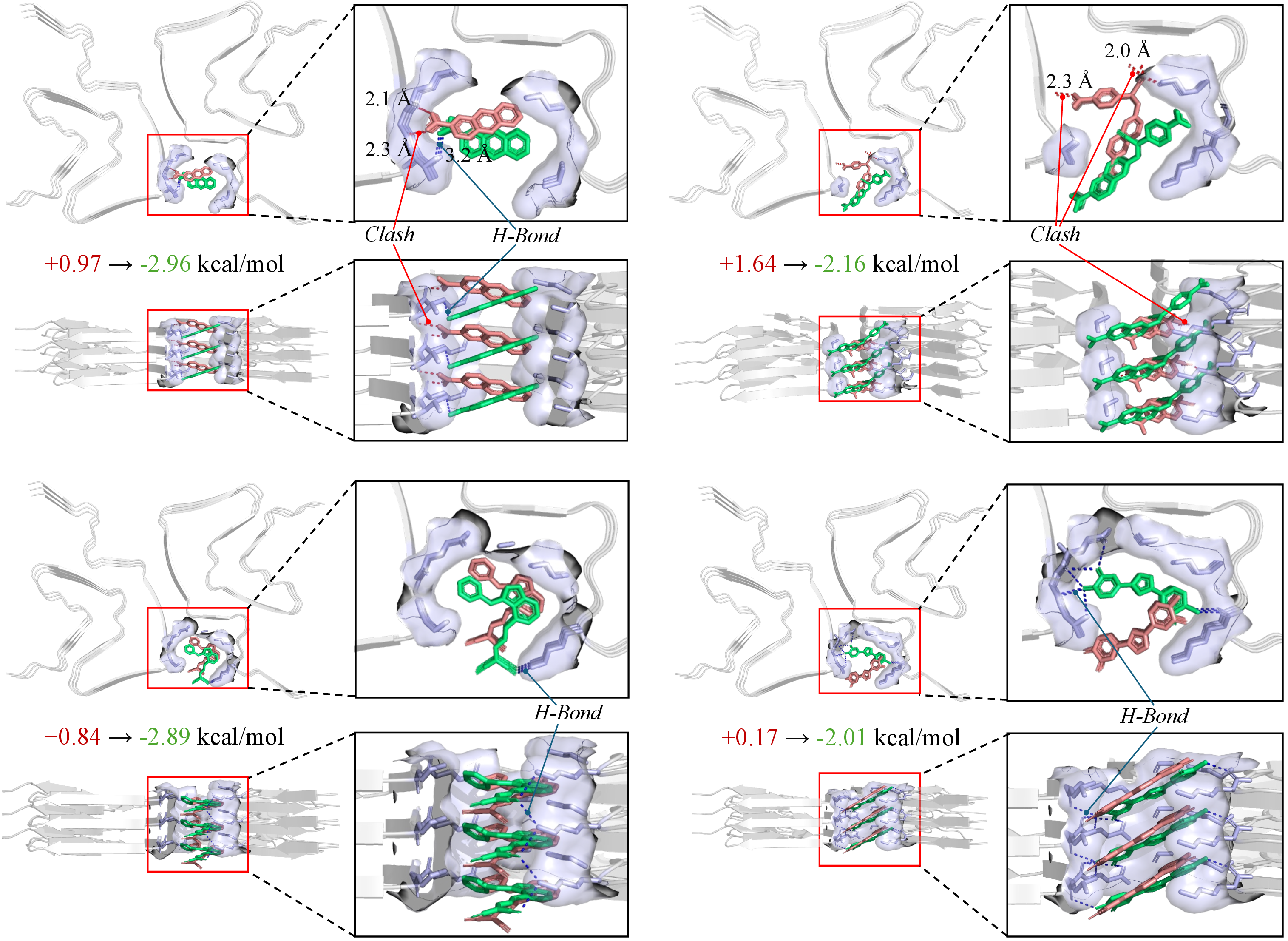
We verify that the RL stage drives the policy toward the cooperative-binding objective at both global and per-complex levels (Figure 8). The mean per-batch reward (left) climbs from a negative initial value to a positive plateau within the first \({\sim}25\) epochs and remains stably positive thereafter, indicating that the policy is being optimised toward the cooperative-binding objective \(r = R_\text{bind} + \lambda R_\text{sym}\). To rule out that this global gain reflects averaging across heterogeneous samples rather than per-complex improvement, we exploit the fact that many training complexes are revisited multiple times during the run and compare \(R_\text{bind}\) at each complex’s last visit against its first (right). Binding energetics become progressively more favourable on \(25\) of \(30\) training complexes (\(83\%\), positive bars, with the largest single-complex improvement reaching \({\sim}9.5\) kcal/mol); the remaining \(5\) complexes show only mild regressions (\(<\!1.5\) kcal/mol) consistent with the inherent stochasticity of on-policy roll-outs. To illustrate what these per-complex energetic gains look like at the pose level, Figure 9 zooms in on four representative complexes from the same set of bars. For each complex, the pose at its first visit during training (brown) fits awkwardly into the cross-\(\beta\) groove and exhibits steric clashes with the protein surface. By the last visit (green), the ligand has adapted to the local pocket geometry, and the resulting shape complementarity yields a richer network of favourable protein–ligand interactions: clashes are eliminated, well-defined hydrogen bonds form, and van der Waals packing improves. \(R_\text{bind}\) correspondingly shifts from positive (unfavourable) to clearly negative values.
7.3 Analysis on Primary Ligand Docking↩︎
To complement the fibril-targeted evaluations in the main paper, we also report CORAL’s behaviour on primary ligand docking, using the leakage-clean 130-target subset of the PoseBusters Benchmark from [36] (PDB deposition date \(>\) 2021-09-30, outside the training cutoff of all deep-learning baselines). The published baselines on the PoseBusters Benchmark each use their best-performing configuration, which for recent cofolding models means inference with multiple-sequence alignments (MSAs). We deliberately train and run CORAL without MSAs: resolved fibril–ligand co-crystal structures are too scarce to yield meaningful evolutionary signal for binding-site geometry, and prior work on amyloid-specific structure prediction further notes that for fibrils MSA acts mainly as a source of stochastic sampling diversity rather than as a coevolutionary prior [10]. Our comparison therefore juxtaposes a no-MSA fibril-specialised framework against general-purpose baselines at their strongest MSA-equipped configurations.
Figure 10 reports our results alongside the published baselines on the PoseBusters Benchmark. After OpenMM ligand relaxation, CORAL achieves \(8.5\%\) RMSD \(\leq 2\) Åand \(7.7\%\) on the joint RMSD \(\leq 2\) Å\(\wedge\) PB-Valid criterion. On exact pose-accuracy metrics our framework trails the strongest MSA-equipped general-purpose baselines (e.g., AlphaFold-3 at \(56.0\%\) RMSD \(\leq 2\) Å); since our warm-up corpus overlaps substantially with these baselines (the same general-purpose docking datasets, augmented with fibril-specific data), the residual gap reflects the contribution of MSA-derived priors that we forgo by design rather than a deficit in training data. Importantly, on the protein–ligand interaction-fingerprint metric PLIF-WM, which scores how well the predicted pose reproduces the chemistry of the native binding-site contacts, our framework is competitive with full AlphaFold-3 (\(52.3\%\) vs \(54.2\%\)), indicating that even without MSAs it recovers the chemically meaningful binding-site contacts on primary ligand targets at a level comparable to the best general-purpose docking baselines.
![Figure 10: ****CORAL** on the PoseBusters Benchmark.** Bars show the percentage of predictions meeting each criterion, with our framework (rightmost) added alongside the seven baselines reported by [36] and run with multiple-sequence alignments disabled. Categories cover pose-accuracy thresholds with and without ligand relaxation (cRMSD \leq 1 Å, RMSD \leq 2 Å, RMSD \leq 2 Å\wedge PB-Valid) and the protein–ligand interaction-fingerprint metric (PLIF-WM, no post-processing).](/article/2607.17412/figures/sup_posebench_fig4_with_ours_130.png "fig:")
8 Additional Qualitative Results↩︎
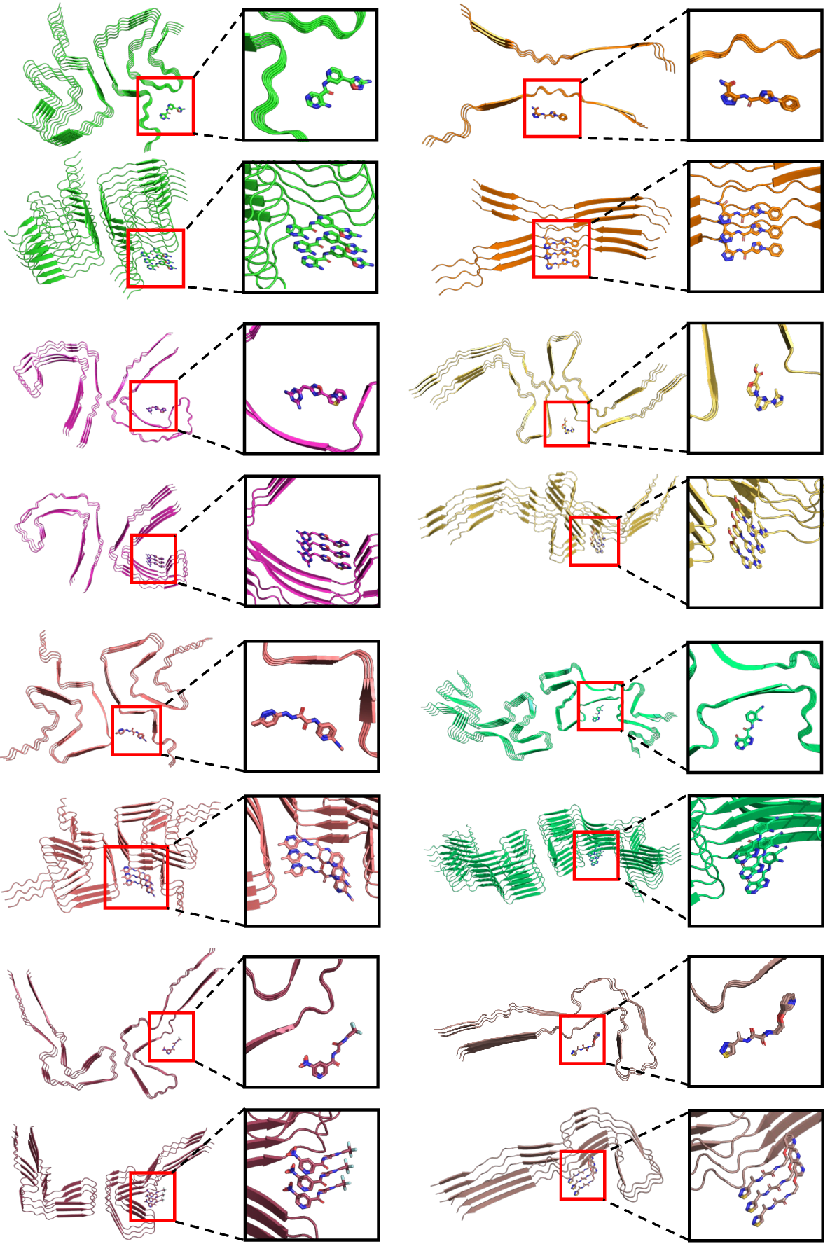
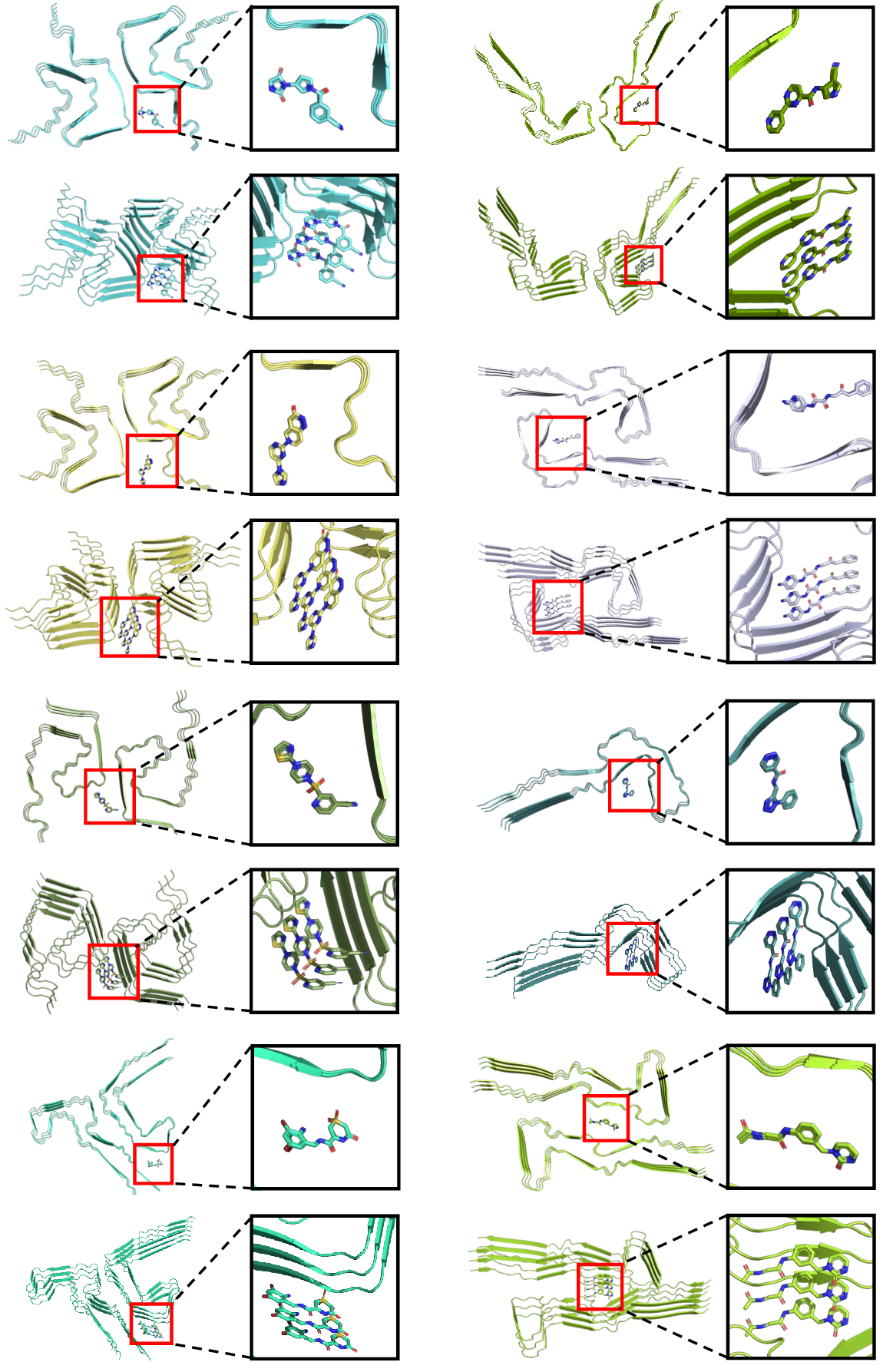
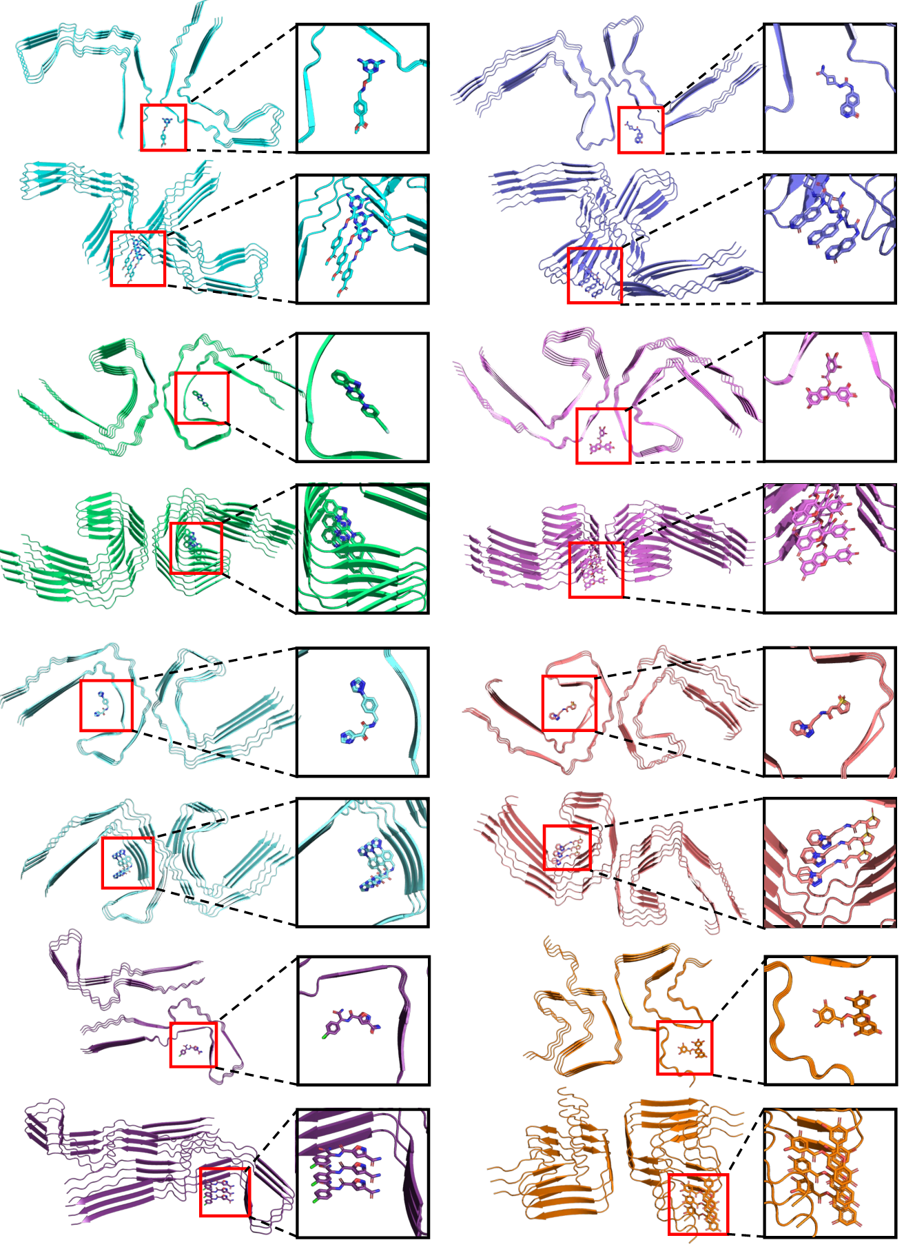
We provide additional qualitative visualisations of CORAL’s predicted fibril–ligand poses on AmyDock-CryoEM and AmyDock-Synthetic targets, complementing the comparisons in §4.2.0.2.