Backpropagation-Free Trunk Training via the Split Forward Gradients
July 18, 2026
Abstract
Backpropagation makes training deep networks memory intensive because it must store intermediate activations. Forward-mode methods avoid this cost, but their gradient estimates become increasingly noisy as the number of trained parameters grows. We introduce Split Forward Gradient (Split-FG), which splits a network at an intermediate representation: it computes the output head gradient exactly and estimates only the trunk gradient with a Jacobian–vector product. This reduces estimator variance and requires no backward pass through the trunk, while retaining an Adam-style convergence guarantee. Our experiments reveal an important practical failure mode. On WikiText-103, naive forward-gradient training of the trunk performs worse than leaving a randomly initialized trunk frozen, likely because Adam updates every noisy, under-determined trunk coordinate too aggressively. Simply using a much smaller learning rate for the trunk reverses this result: a \(16\)M-parameter GPT-2-style model reaches validation perplexity \(387\), compared with \(668\) for the frozen-trunk control and \(2{,}885\) for a matched pure forward-gradient baseline (backpropagation reaches \(150\)). Split-FG also produces the strongest backprop-free results on our tabular benchmarks and reaches \(60.5\%\) on CIFAR-10 and \(35.2\%\) on CIFAR-100 with a heavy-head design. It reduces peak memory by up to \(35\%\) relative to matched backpropagation, although the performance gap widens as the forward-mode trunk grows.
1 Introduction↩︎
The computational cost of training deep neural networks is dominated by backpropagation [1]: the reverse-mode differentiation of a loss through the entire network via the chain rule. This requires storing the full computational graph and all intermediate activations in memory—a cost that scales linearly with network depth and sequence length: at roughly \(16\,d_{\mathrm{model}}\) bytes per token per layer (half precision), a \(32\)-layer, \(d_{\mathrm{model}}{=}4096\) model at sequence length \(4096\) and batch size \(8\) holds \({\approx}69\) GB of activations alone, beyond a single \(80\) GB accelerator once weights and optimizer state are added. These requirements are obstacles for deployment on resource-constrained hardware, for continual learning systems that update parameters online, and for models of biological learning, where symmetric backward error transport through deep stacks is considered implausible (though our own exact head still uses weight transport at its single readout layer). A sharper case than cost is hardware where the backward pass is not merely expensive but unavailable: optical and analog accelerators run the forward pass natively at very low energy [2], but backpropagating through them requires the adjoint method—reverse field propagation with in-situ measurement, or an accurate digital twin [3]. What such hardware admits is gradient information from forward evaluations alone, directional derivatives obtained by perturb-and-measure, with no reverse pass through the physical stack-, which is precisely the regime the method developed for backpropagation-free targets.
Prior work on backpropagation-free training has demonstrated promising results on small-scale tasks. Forward gradients via JVP [4] and evolution strategies [5], [6] provide unbiased gradient estimates but suffer from variance that scales linearly with parameter count. Zeroth-order methods such as MeZO [7] can fine-tune pretrained language models but struggle with pretraining from scratch. Equilibrium propagation [8], [9] and predictive coding [10]–[12] match backpropagation on shallow networks through local energy minimisation, but require iterative settling phases that multiply per-step cost. The Forward-Forward algorithm [13] replaces the backward pass with contrastive positive/negative phases per layer, though it has only been validated on small classifiers. Direct feedback alignment [14] and local learning rules [15] reduce inter-layer dependence but introduce bias through fixed random projections or surrogate losses. Despite this breadth, a persistent gap remains: these methods degrade when scaled to transformers, need a pretrained initialisation, or introduce systematic bias through approximate objectives.
In this paper we show that decomposing the gradient computation at an intermediate representation substantially reduces forward-gradient variance and recovers part of the gap to backpropagation, with no backward pass through the trunk. The strict, unclipped estimator is unbiased; our runs apply global gradient clipping, and the GPT runs additionally train the tied vocabulary table through a readout-only surrogate (Appendices 9 and 12.7). We call the estimator Split Forward Gradient (Split-FG) and make the following contributions.
The Split-FG estimator. We decompose the forward gradient at any intermediate representation \(h\), compute the head-side gradient \(\partial\mathcal{L}/\partial h\) in closed form (or estimate it in low dimension), and restrict the stochastic forward gradient to the trunk. The directional derivative is exact with respect to the head, so only the trunk contributes noise. We evaluate the Split-FG estimator on tabular, image, and language tasks and shows its superiority over many backpropagation free baselines.
A measured variance analysis. We show that the Split-FG estimator enables per-coordinate estimator variance to drop from \(\lVert\nabla_{\theta}\mathcal{L}\rVert^2\) to \(\lVert\nabla_{\theta_{\mathrm{trunk}}}\mathcal{L}\rVert^2\), and we measure this factor rather than assuming it. On our GPT configuration, where the vocabulary readout holds \(80\%\) of the parameters, the trunk carries \(0.74\) of the gradient energy at initialisation, giving a \(1.35\times\) per-coordinate and \(6.8\times\) total variance reduction (Section 2.2). The exact head gradients are available in closed form for linear cross-entropy and MSE heads, and for a factored two-linear head, so the pipeline uses no reverse-mode automatic differentiation.
An empirical failure mode and its fix. Using a frozen-trunk control that trains only the exact head over a fixed random trunk, we find that naive forward-gradient training of the trunk is worse than not training it at all (\(1733\) versus \(668\) perplexity on WikiText-103). We attribute this to Adam, which steps every noisy, under-determined trunk coordinate at full length. Scaling the trunk step down by a factor \(\rho=0.03\) removes the failure: a \(16\)M-parameter GPT-2-style transformer trained from scratch reaches perplexity \(387\), which is \(42\%\) below the frozen control and \(7.5\times\) below a pure forward-gradient baseline matched in tangent count and tuning (\(2{,}885\) at \(K{=}4\)). In these validation runs it uses \(35\%\) less peak memory than the same-architecture Adam backpropagation reference (which reaches \(150\)), but takes \(3.2\times\) longer per step.
The remainder of the paper is organized as follows. Section 2 develops Split-FG and its variance analysis; Section 3 gives a convergence guarantee for a predictable-preconditioner idealisation of the split estimator. Section 4 compares Split-FG with backpropagation and no-trunk-backward baselines across tabular, image, and GPT-style language-modelling tasks, where a frozen-trunk control isolates the trunk’s contribution and motivates the trunk-step fix (Section 4.4; Appendix 12.2), followed by ablation studies. Section 5 discusses limitations and future directions. Code for all experiments is provided in the supplementary material.
2 Preliminaries↩︎
2.1 Forward Gradient↩︎
Consider a neural network parameterised by \(\theta \in \mathbb{R}^P\) with scalar loss \(\mathcal{L}(\theta)\). For a direction vector \(v \in \mathbb{R}^P\), the directional derivative is the scalar \[\label{eq:dir-deriv} d \;=\; \nabla_{\theta}\mathcal{L}(\theta) \cdot v \;=\; \sum_{j=1}^{P} \frac{\partial \mathcal{L}}{\partial \theta_j}\, v_j\,.\tag{1}\] This can be computed exactly, without a backward pass, via a Jacobian-vector product (JVP) using forward-mode automatic differentiation [16]. The JVP augments each intermediate variable with a tangent and propagates both jointly through the computation graph via dual-number arithmetic; initialising the tangent of \(\theta\) to \(v\) yields the pair \((\mathcal{L},\, d)\) in a single pass. The computational cost is comparable to one forward evaluation; crucially, no activations need to be stored for a backward pass. Writing \(g := \nabla_{\theta}\mathcal{L}(\theta)\) with coordinates \(g_i\), [4] observe that if \(v \sim \mathcal{N}(0, I_P)\), the product \(d \cdot v\) is an unbiased estimate of the full gradient: \[\label{eq:fg-estimator} \hat{g} = d \cdot v\,, \qquad \mathbb{E}[\hat{g}] = g\,.\tag{2}\] Unbiasedness is immediate from \(\mathbb{E}[v\,v^\top] = I\); the per-coordinate computation appears in Appendix 7. With \(K\) independent samples \(\{v_k\}_{k=1}^{K}\), the averaged estimator \[\label{eq:fg-K} \hat{g}^{(K)} = \frac{1}{K} \sum_{k=1}^{K} d_k\, v_k\tag{3}\] retains unbiasedness. Its per-coordinate variance follows from Isserlis’ theorem [17] on fourth-order Gaussian moments: since \(\mathbb{E}[v_j\,v_k\,v_i\,v_i] = \delta_{jk} + 2\,\delta_{ji}\,\delta_{ki}\), we obtain \[\label{eq:fg-variance} \mathrm{Var}\bigl[\hat{g}^{(K)}_i\bigr] = \frac{1}{K}\Bigl( \lVert g \rVert^2 + g_i^2 \Bigr)\,.\tag{4}\] The dominant term \(\lVert g\rVert^2 = \sum_{j=1}^{P} g_j^2\) sums over all \(P\) parameters, yielding a signal-to-noise ratio for \(i\)-th coordinate: \[\label{eq:snr} \mathrm{SNR}_i = \frac{g_i^2}{\lVert g\rVert^2} \;\approx\; \frac{1}{P}\,.\tag{5}\] For a model with \(P = 10^7\) parameters, each coordinate’s signal is overwhelmed by noise from the remaining \(P - 1\) coordinates. This linear scaling of variance with parameter count is the fundamental barrier to applying forward gradients at scale, and motivates the decomposition we introduce in Section 2.2.
2.2 Split Forward Gradient↩︎
The core identity underlying Split-FG is easiest to read as an algorithmic “push–score–estimate” chain rule at an intermediate representation \(h = f(x;\,\theta_{\mathrm{trunk}}) \in \mathbb{R}^{d_h}\). Algorithm 1 spells out the estimator. For each random direction in trunk-parameter space, we first push the direction to the representation space, score the resulting representation perturbation by the loss gradient at \(h\), and then place that scalar back on the same random direction.
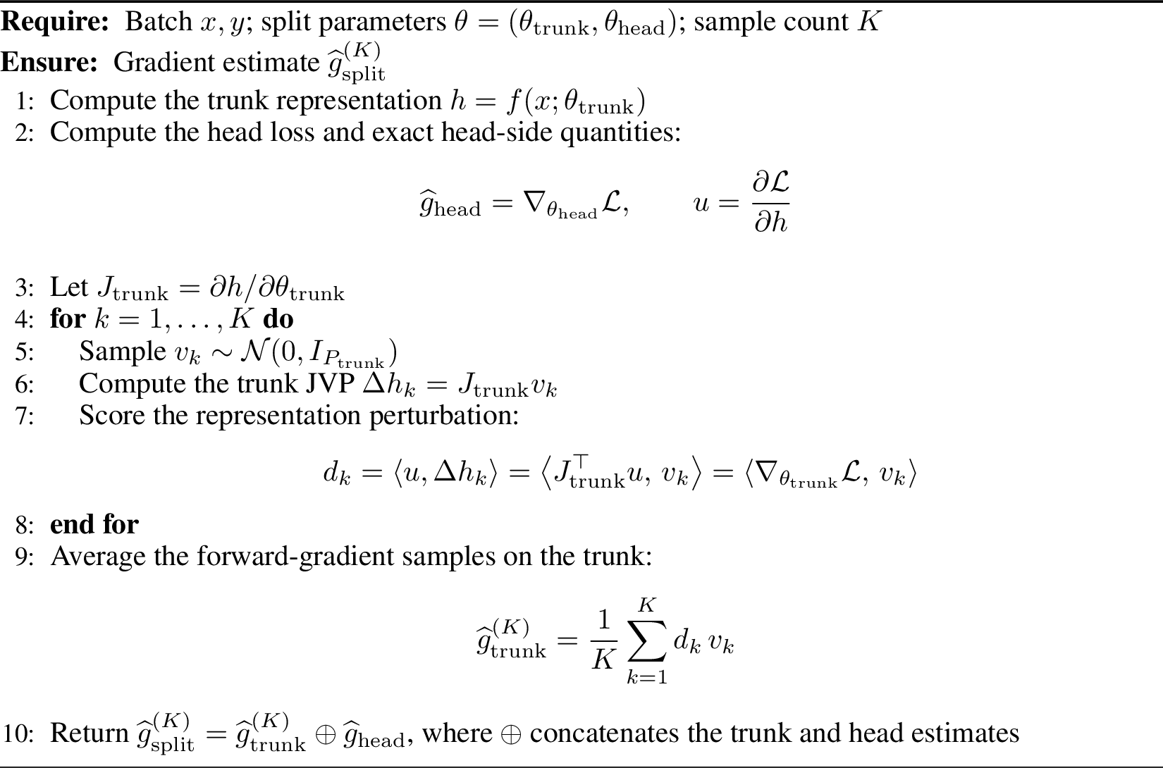
The standard forward gradient draws \(v\in\mathbb{R}^{P_{\mathrm{total}}}\) and estimates all parameters from one noisy scalar; Split-FG restricts the random directions to the trunk subspace and computes the head gradient exactly. The chain-rule equality in the score step of Algorithm 1 is the justification only: the implementation computes each \(d_k\) from \(u = \partial\mathcal{L}/\partial h\) and \(\Delta h_k\), so no backward pass through the trunk ever occurs. Appendix 7 shows the estimator in Algorithm 1 yields a per-coordinate variance reduction of \[\label{eq:variance-reduction} \frac{ \mathrm{Var}\!\bigl[\hat{g}_i^{\;\mathrm{split}}\bigr] }{ \mathrm{Var}\!\bigl[\hat{g}_i^{\;\mathrm{standard}}\bigr] } \;\approx\; \frac{ \bigl\lVert \nabla_{\theta_{\mathrm{trunk}}}\mathcal{L} \bigr\rVert^2 }{ \bigl\lVert \nabla_{\theta}\mathcal{L} \bigr\rVert^2 } \;\approx\; \frac{P_{\mathrm{trunk}}}{P_{\mathrm{total}}}\tag{6}\] where the first relation is leading-order (it drops the \(O(g_i^2)\) diagonal terms; the exact per-coordinate identities are derived in Appendix 7) and the final approximation holds when gradient magnitudes are approximately uniform across parameters. The trunk and head parameters partition the network, \(P_{\mathrm{total}} = P_{\mathrm{trunk}} + P_{\mathrm{head}}\), so the ratio \(P_{\mathrm{trunk}}/P_{\mathrm{total}} = P_{\mathrm{trunk}}/(P_{\mathrm{trunk}} + P_{\mathrm{head}})\) is small precisely when the head holds most of the weights.
Equation equation 6 exposes the single lever that governs Split-FG: the estimator is effective precisely when the forward-mode trunk holds few parameters relative to the exactly differentiated head (\(P_{\mathrm{trunk}} \ll P_{\mathrm{head}}\)). Language models satisfy this for free through their large vocabulary readouts. The same lever separates Split-FG from the closest prior variance-reduction program: [15] also shrink the perturbed dimension, but with layer-local losses at the price of a surrogate objective; Split-FG keeps the global loss and removes the head’s share exactly. The adversarial case is a light head over a heavy trunk, which is most notably a plain convolutional network making the variance ratio approaches one and Split-FG degrades to standard forward gradient; the resolution is to restructure the network around a small forward-mode feature extractor and a large exact head, the inversion we adopt for image classification (Section 4.3). The same light trunk also minimizes forward-mode activation memory (Appendix 11.1), so the heavy-head/light-trunk principle improves accuracy and memory together.
2.3 Parameter Update Rule↩︎
Split-FG uses exact gradients for the head and forward-gradient estimates for the trunk, then updates both parameter sets with Adam.
Let’s first recall the gradient of head parameters. For a linear head \(\mathrm{logits} = h\,W_{\mathrm{head}}^\top + b\) with cross-entropy loss, the gradients are available in closed form: \[\label{eq:head-grads} \frac{\partial \mathcal{L}}{\partial b} = \frac{1}{N}\sum_{n}\bigl(p_n - \mathbf{1}_{y_n}\bigr), \qquad \frac{\partial \mathcal{L}}{\partial W_{\mathrm{head}}} = \tfrac{1}{N}\bigl(p - \mathbf{1}_{y}\bigr)^{\!\top} h, \qquad \frac{\partial \mathcal{L}}{\partial h} = \tfrac{1}{N}\bigl(p - \mathbf{1}_{y}\bigr) W_{\mathrm{head}},\tag{7}\] Here \(p = \mathrm{softmax}(\mathrm{logits})\), \(\mathbf{1}_{y}\) is the one-hot target matrix, and \(N=BT\) is the number of token positions. These are the usual one-layer head derivatives, computed directly rather than with an autodiff tape. Split-FG eliminates reverse-mode differentiation through the trunk, not through the head.
As to the trunk parameters, where the forward gradient comes into play, we compute a trunk JVP and its directional derivative for \(K\) random tangent vectors \(v_k \sim \mathcal{N}(0, I_{P_{\mathrm{trunk}}})\), : \[\label{eq:trunk-grad-est} \Delta h_k = \frac{\partial h}{\partial \theta_{\mathrm{trunk}}}\, v_k, \qquad d_k = \Bigl\langle \frac{\partial \mathcal{L}}{\partial h},\, \Delta h_k \Bigr\rangle, \qquad \hat{g}_{\mathrm{trunk}} = \frac{1}{K} \sum_{k=1}^{K} d_k \, v_k ,\tag{8}\] Each tangent requires one JVP and one inner product. The estimator is unbiased because \(\mathbb{E}[v v^\top]=I\).
Next, we use bias-corrected Adam [18], with the exact head gradient and the trunk estimate in Eq. equation 8 . Its per-coordinate normalization handles the scale mismatch between head gradients of magnitude \(O(1)\) and trunk estimates with variance \(O(P_{\mathrm{trunk}}/K)\). However, it does not account for each coordinate’s signal-to-noise ratio, so noisy trunk coordinates can still receive overly large updates. For large trunks, we therefore use a separate trunk step scale (Section 4.4). Adam, AdamW, and Muon work in our ablations, whereas SGD forward gradients remain at the random-prediction floor on WikiText-103; even tuned pure FG with Adam is \(7.5\times\) worse than Split-FG (Table ¿tbl:tab:main-lm?).
3 Convergence analysis for a predictable preconditioner↩︎
In this section we will provide a theoretical support for the convergence of Split-FG under Adam. Throughout this section \(F(\theta)\) denotes the full-batch training objective, i.e.the loss \(\mathcal{L}\) of Section 2 evaluated on the full training set. The Split-FG estimator of Section 2.2 is conditionally unbiased for \(\nabla F(\theta)\) when the loss is evaluated full-batch; minibatch sampling adds only the standard data-noise term, handled at the end of Appendix 8. For simplicity, we analyse the idealised update \(\theta_{t+1}=\theta_t-\eta A_t\hat{g}_t\), where \(\hat{g}_t\) is the Split-FG estimator (exact head, \(K\)-tangent trunk) and \(A_t\) is a diagonal preconditioner, under the following assumptions.
Assumption 1 (Regularity). \(F\) is differentiable and \(L\)-smooth, and bounded below: \(F(\theta)\ge F_\star>-\infty\) for all \(\theta\).
Assumption 2 (Predictable, bounded preconditioner). \(A_t=\mathrm{diag}(a_{t,1},\dots,a_{t,P_{\mathrm{total}}})\) is predictable—measurable with respect to the history \(\mathcal{F}_t\) fixed before the step-\(t\) tangents are drawn—and satisfies \(0<a_{\min}\le a_{t,i}\le a_{\max}<\infty\) for all \(t,i\).
Assumption 3 (Unbiasedness and bounded adaptive noise). The estimator is conditionally unbiased, \(\mathbb{E}_t[\hat{g}_t]=\nabla F(\theta_t)\), and its adaptive noise ratio \(R_t(A_t)=\mathbb{E}_t[\lVert A_t\hat{g}_t\rVert^2]\big/ \langle\nabla F(\theta_t),A_t\nabla F(\theta_t)\rangle\) (set to \(0\) when \(\nabla F(\theta_t)=0\)) obeys \(R_t(A_t)\le R_{\max}\) almost surely.
Theorem 1 (Predictable-preconditioner Split-FG). Under Assumptions 1–3, if \(0<\eta\le \frac{1}{L R_{\max}}\) then for every horizon \(T\ge1\) \[\frac{1}{T}\sum_{t=0}^{T-1} \mathbb{E}\big[\langle\nabla F(\theta_t),A_t\nabla F(\theta_t)\rangle\big] \;\le\;\frac{2\,(F(\theta_0)-F_\star)}{\eta\,T},\] and consequently \(\tfrac{1}{T}\sum_{t=0}^{T-1}\mathbb{E}\lVert\nabla F(\theta_t)\rVert^2 \le 2(F(\theta_0)-F_\star)/(\eta\,a_{\min}T)\). The Split-FG estimator satisfies \(R_{\max}\le(a_{\max}^2/a_{\min})\big(1+(P_{\mathrm{trunk}}+1)/K\big)\), so the step-size condition is always feasible; the guarantee is the standard \(O(1/T)\) rate for nonconvex first-order stationarity.
Theorem 1 certifies descent in the geometry chosen by the preconditioner: the stationarity measure is the preconditioned gradient energy \(\langle\nabla F,A_t\nabla F\rangle\), and the head coordinates contribute no variance term because they are updated exactly. It guarantees convergence, not the quality of the point reached within a finite budget—the second-moment denominator equalises update magnitudes but does not distinguish signal from noise, and Section 4.4 shows that at large \(P_{\mathrm{trunk}}\) a further trunk-specific step scale \(\rho\) is needed. That variant is covered unchanged, since scaling the trunk entries of \(A_t\) by a constant \(\rho\) preserves Assumption 2. The proof, the exact weighted second moment underlying the \(R_{\max}\) bound, and an unpreconditioned SGD counterpart are in Appendix 8.
4 Experiments↩︎
This section is designed to test Split-FG as a general training principle, not only as a language-model trick. We organize the experiments around four questions. First, does the estimator variance follow the scaling predicted by Eq. equation 6 ? Second, does Split-FG work with different loss functions, including cross-entropy classification and MSE regression? Third, does the method transfer across modern tabular, vision, and language architectures? Fourth, which design choices matter most in GPT-style transformers?
4.0.0.1 Protocol and metrics.
Tabular and GPT experiments pair Split-FG with a same-architecture backpropagation reference under the same data-exposure budget. The headline image table instead compares separately structured systems and, on CIFAR-100, method-specific budgets; its architecture-matched flat-head ablation is reported separately. Each large experiment reports peak GPU memory together with the reference difference \(\mathrm{MemSave}=1-M_{\mathrm{peak}}(\text{Split-FG})/M_{\mathrm{peak}}(\text{Backprop})\). The full training and memory-measurement protocol is given in Appendix 9.
4.0.0.2 No-global-backward baselines.
Beyond pure forward gradient and antithetic ES, we compare—wherever they apply against Forward-Forward [13] (layer-local goodness training; classification only), predictive coding [10], [11] (local error settling with Hebbian updates), and a training-free modern-Hopfield associative memory [19] (softmax retrieval over a frozen trunk; kNN-LM style [20] for language modelling). All three use zero JVPs and zero trunk backward passes; their mechanisms and per-domain configurations are detailed in Appendix 9 and the per-domain protocol appendices.
4.1 Toy Illustration: Variance at the Split↩︎
We first construct a toy model in which the total parameter vector can be partitioned into a large linear head and a small nonlinear trunk. The model has the form \[h = f(x;\theta_{\mathrm{trunk}}), \qquad \hat{y} = W_{\mathrm{head}}h + b ,\] with squared loss or cross-entropy loss depending on the output type. This setting allows us to measure the true gradient exactly and compare the empirical variance of three estimators: standard forward gradient over all parameters, Split-FG with an exact head gradient, and backpropagation. We vary the head dimension while holding the trunk fixed, so that \(P_{\mathrm{head}}/P_{\mathrm{trunk}}\) can be swept directly.
We instantiate this diagnostic with a two-layer ReLU MLP trunk (\(P_{\mathrm{trunk}}=1600\)) and a linear cross-entropy head whose class count \(C\in\{50,500,5000\}\) grows the head from \(1650\) to \(165000\) parameters at fixed trunk; for each \(C\) we draw \(2000\) single-direction (\(K{=}1\)) estimates against the exact minibatch gradient and report variance over the trunk coordinates (the analytical head contributes none). Full protocol in Appendix 7.
For Gaussian tangents, the leading-order variance-ratio prediction on a fixed minibatch is \[\label{eq:toy-energy-ratio} \frac{ \mathrm{Var}[\hat{g}^{\mathrm{split}}_{\mathrm{trunk}}] }{ \mathrm{Var}[\hat{g}^{\mathrm{pure}}_{\mathrm{trunk}}] } = \frac{ \|\nabla_{\theta_{\mathrm{trunk}}}\mathcal{L}\|_2^2 }{ \|\nabla_{\theta}\mathcal{L}\|_2^2 } .\tag{9}\] The parameter-count ratio \(P_{\mathrm{trunk}}/P_{\mathrm{total}}\) is thus a uniform-gradient-energy approximation, not an identity. This distinction matters in the toy classifier: as the number of classes grows, the count ratio becomes very small, but the observed ratio follows the gradient-energy prediction.
The toy result (Figure 3 and Table ¿tbl:tab:toy-variance?, Appendix 7) supports the core variance mechanism while also clarifying what should be compared in finite models. Split-FG consistently reduces the trunk-coordinate variance relative to pure forward gradient, and the measured ratios are within \(6.8\%\) of Eq. equation 9 across the sweep. Backpropagation is included only as the zero-variance reference: it supplies the exact gradient used to evaluate estimator variance, but it is not a stochastic estimator.
4.2 Tabular Learning with TabM-Style Models↩︎
The tabular experiments test both architectural generality and loss-function generality. We use a TabM-style parameter-efficient ensemble model, with feature preprocessing, a shared MLP trunk, and multiple prediction heads or submodel outputs. For classification datasets, the final layer uses cross-entropy and the analytical head gradient from Eq. equation 7 . For regression datasets, the final layer uses MSE, whose closed-form head gradient mirrors Eq. equation 7 (Appendix 10.3).
The dataset subset follows the spirit of the TabM [21] benchmark while keeping the experiment time reasonable; the datasets are drawn mainly from OpenML. Full dataset and protocol details are in Appendix 10, and the network structure in Appendix 10.3.
| Dataset | Task | Loss | Backprop | Pure FG | ES | FF | PC | Hop. | Split-FG |
|---|---|---|---|---|---|---|---|---|---|
| Adult | bin. cls. | CE | \(84.2_{\pm0.5}\) | \(81.7_{\pm0.1}\) | \(81.8_{\pm0.1}\) | \(81.6_{\pm0.5}\) | \(81.5_{\pm0.4}\) | \(79.1_{\pm0.4}\) | \(\textbf{82.5}_{\pm0.4}\) |
| Higgs Small | bin. cls. | CE | \(68.8_{\pm0.7}\) | \(59.0_{\pm0.6}\) | \(59.0_{\pm0.6}\) | \(61.7_{\pm0.4}\) | \(61.5_{\pm0.4}\) | \(55.4_{\pm0.3}\) | \(\textbf{61.9}_{\pm0.3}\) |
| Otto | multicls. | CE | \(78.3_{\pm0.4}\) | \(62.8_{\pm0.6}\) | \(62.8_{\pm0.6}\) | \(30.8_{\pm3.5}\) | \(68.8_{\pm0.4}\) | \(62.3_{\pm0.7}\) | \(\textbf{71.7}_{\pm0.4}\) |
| Covertype | multicls. | CE | \(71.7_{\pm0.5}\) | \(61.2_{\pm0.2}\) | \(61.2_{\pm0.2}\) | \(35.0_{\pm2.2}\) | \(65.5_{\pm0.6}\) | \(62.1_{\pm1.1}\) | \(\textbf{66.8}_{\pm0.6}\) |
| California | reg. | MSE | \(0.491_{\pm0.013}\) | \(0.595_{\pm0.012}\) | \(0.595_{\pm0.012}\) | – | \(0.638_{\pm0.015}\) | \(0.755_{\pm0.014}\) | \(\textbf{0.564}_{\pm0.016}\) |
| House 16H | reg. | MSE | \(0.652_{\pm0.024}\) | \(0.829_{\pm0.027}\) | \(0.829_{\pm0.027}\) | – | \(0.838_{\pm0.033}\) | \(0.859_{\pm0.040}\) | \(\textbf{0.773}_{\pm0.030}\) |
| Diamond | reg. | MSE | \(0.249_{\pm0.004}\) | \(0.334_{\pm0.006}\) | \(0.334_{\pm0.006}\) | – | \(0.452_{\pm0.001}\) | \(0.490_{\pm0.003}\) | \(\textbf{0.311}_{\pm0.004}\) |
| Black Friday | reg. | MSE | \(0.809_{\pm0.006}\) | \(0.906_{\pm0.003}\) | \(0.906_{\pm0.003}\) | – | \(0.901_{\pm0.004}\) | \(0.938_{\pm0.005}\) | \(\textbf{0.890}_{\pm0.006}\) |
Across all eight default datasets, Split-FG consistently improves over the evaluated pure forward-gradient and ES controls under \(5\)-fold cross-validation (paired \(t\)-tests)—e.g.on Otto it lifts accuracy from \(62.8\%\) to \(71.7\%\) against a \(78.3\%\) backprop reference. On Higgs its lead over Forward-Forward is within the cross-validation spread. Split-FG also lowers peak training memory on every dataset measured (\(4.3\)–\(24.1\%\); Table ¿tbl:tab:tabular-memory? in the appendix).
4.3 Image Classification↩︎
Convolutional networks are the adversarial case for Split-FG (Section 2.2): a ResNet holds almost all of its parameters in the convolutional trunk and only a thin linear head, so a naive split must forward-estimate the whole trunk and degrades to standard forward gradient. We therefore apply the heavy-head/light-trunk restructuring: for CIFAR-10 we keep only the first residual block of a ResNet-20 (GroupNorm) as the forward-mode trunk (\(5{,}136\) parameters, under \(2\%\) of the backbone) and attach a large exact head that flattens its feature map and maps it to the logits through a two-layer linear factorisation, \[h = \mathrm{ResBlock}_1(x;\theta_{\mathrm{trunk}}) \in \mathbb{R}^{16384}, \qquad \mathrm{logits} = W_2 (W_1 h) + b ,\] trained by an exact closed-form gradient (pure matrix products, no reverse-mode backward pass through the trunk). Although \(W_2 W_1\) collapses to a single linear map, training the factored pair yields a deep-linear over-parameterisation effect worth \(+2.5\) points over a single exact linear head (\(p<0.01\); Appendix 11.3). The inner width is \(H{=}64\), so \(W_1\in\mathbb{R}^{H\times16384}\) and \(W_2\in\mathbb{R}^{C\times H}\) for \(C\) classes; we use \(K{=}4\) tangents (\(H{=}128\) for CIFAR-100, which uses a stronger ResNet-18 backbone). The baselines use the dataset’s standard backbone: Pure FG and ES estimate the full network, Forward-Forward (FF) and predictive coding (PC) run on flattened images, and Hopfield (Hop.) is an associative-memory readout over a frozen trunk. Dataset, protocol, and architecture details are given in Appendices 11–11.2.
| Dataset | Backprop | Pure FG | ES | FF | PC | Hop. | Split-FG |
|---|---|---|---|---|---|---|---|
| CIFAR-10 | \(88.2_{\pm0.6}\) | \(29.5_{\pm1.9}\) | \(29.3_{\pm1.4}\) | \(48.8_{\pm0.4}\) | \(40.7_{\pm1.1}\) | \(10.0_{\pm0.0}\) | \(60.5_{\pm1.2}\) |
| CIFAR-100 | \(65.6_{\pm1.0}\) | \(1.2_{\pm0.2}\) | \(1.2_{\pm0.1}\) | \(6.9_{\pm0.5}\) | \(1.0_{\pm0.0}\) | \(1.4_{\pm0.3}\) | \(35.2_{\pm0.5}\) |
In the reported five-seed CIFAR-10 development results, the restructured Split-FG system reaches \(60.5\%\) after \(60\) epochs (Table ¿tbl:tab:image-main?), compared with \(29.5\%\) for full-ResNet pure FG and \(48.8\%\) for the separately structured Forward-Forward system; because these methods use different architectures, this does not isolate an estimator effect. Split-FG is \(27.7\) points below the full ResNet-20 backpropagation reference (\(88.2\%\)). Published no-global-backward pipelines with heavier machinery reach far higher. For example, DeepZero [22] attains \({\sim}86\%\) on CIFAR-10 with sparse zeroth-order training of a full ResNet-20 at substantially larger compute. Table ¿tbl:tab:image-main? should therefore be read as preliminary system evidence, not a state-of-the-art or matched-method comparison. The exact head is what makes the split work: forward-estimating it instead collapses accuracy from \(56.9\%\) to \(\approx\!22\%\) in the matched ablation of Appendix 11.3. The light trunk also cuts peak memory to \(1282\) MiB, below backpropagation’s \(1520\) MiB and reversing the \(2668\) MiB blow-up of the naive full-trunk split (Table ¿tbl:tab:image-memory?). On CIFAR-100, the \(60\)-epoch Split-FG system reaches \(35.2_{\pm0.5}\%\) and the \(60\)-epoch ResNet-18 backpropagation reference reaches \(65.6_{\pm1.0}\%\). The remaining methods were stopped at the same budgets, so their numbers support a matched-budget ranking.
4.4 GPT-Style Language Modelling↩︎
The main stress test is GPT-2-style causal language modelling from random initialisation on WikiText-103, a standard real-text benchmark. The model is a causal transformer (token and positional embeddings, GPT blocks, final normalisation, linear LM
head); the default split is before the LM head: \[h = \mathrm{GPT}_{\mathrm{trunk}}(x;\theta_{\mathrm{trunk}}), \qquad \mathrm{logits}=hW_{\mathrm{out}}^\top+b .\] We report single-seed validation NLL and perplexity, mean
step time, and peak GPU memory; the tangent-count ablation in Appendix 12.6 additionally reports JVPs per step. The same-architecture Adam backpropagation and Split-FG runs use the same number of training tokens
and optimizer updates. The concrete small8 architecture (\(4\) layers, \(d_{\mathrm{model}}=256\), \(16.1\)M parameters) is listed in
Table ¿tbl:tab:gpt-arch?, and the full protocol in Appendix 12.1.
Table ¿tbl:tab:main-lm? compares three Split-FG settings: a naive run that uses Adam’s full step for the trunk (perplexity \(1733.4\)), a frozen-trunk control that trains only the exact head (\(667.6\)), and a run with the trunk step scaled by \(\rho=0.03\) (\(386.7\)). Unless noted otherwise, FG and ES use one tangent. The \(K{=}4\) pure-FG baseline is learning-rate tuned using the screening protocol in Appendix 12.1. The backpropagation reference uses Adam without weight decay; a separately tuned AdamW run reaches \(75.5\) perplexity. Hopfield time denotes a full retrieval pass.
The naive run performs worse than freezing the trunk. We believe this is because the unbiased trunk estimate still has very low per-coordinate signal-to-noise ratio (\({\sim}1/P_{\mathrm{trunk}}\); Eq. equation 5 ). Adam therefore gives full-sized updates to many weakly determined trunk coordinates, which can cause the trunk to drift before its signal accumulates. Reducing the trunk step by \(\rho\!\ll\!1\) limits this noise-driven drift while preserving the slower, coherent update. At matched \(K{=}4\), this simple change improves perplexity by \(4.5\times\) with the same peak memory and essentially unchanged step time. Figure 2 shows the training curves; further frozen-trunk and trunk-scale controls are in Appendix 12.2.
| Method | Train exposure | Val. NLL | PPL | Time | Peak mem. |
|---|---|---|---|---|---|
| Same-architecture backprop + Adam | \(119.1\)M / \(1\) ep. | \(\mathbf{5.0080}\) | \(\mathbf{149.61}\) | \(41.7\) ms | \(1237.7\) MiB |
| Forward gradient + Adam, \(K{=}1\) | same | \(10.5999\) | \(40128.90\) | \(63.6\) ms | \(1038.4\) MiB |
| Forward gradient + Adam, \(K{=}4\), tuned lr | same | \(7.9673\) | \(2884.97\) | \(137.4\) ms | \(1694.5\) MiB |
| Forward gradient + SGD, \(K{=}1\) | same | \(10.8274\) | \(50385.05\) | \(54.6\) ms | \(913.7\) MiB |
| Antithetic ES + Adam, \(K{=}1\) | same | \(9.4012\) | \(12103.11\) | \(44.1\) ms | \(764.7\) MiB |
| Hopfield assoc.memory (kNN-LM) | \(4096\) windows | \(7.4466\) | \(1714.02\) | \(48.5\) s | \(5368.1\) MiB |
| Unigram reference (count-based) | train counts | \(7.4140\) | \(1659.03\) | — | — |
| Interpolated bigram reference | train counts | \(5.2889\) | \(198.12\) | — | — |
| Split-FG + Adam, \(K{=}4\), naive trunk step (\(\times1\)) | \(119.1\)M / \(1\) ep. | \(7.4578\) | \(1733.36\) | \(137.3\) ms | \(810.6\) MiB |
| Frozen trunk \(+\) exact head (\(K{=}0\)) | \(119.1\)M / \(1\) ep. | \(6.5037\) | \(667.64\) | \(24.4\) ms | \(810.6\) MiB |
| Split-FG + Adam, \(K{=}4\), trunk step \(\times0.03\) | \(119.1\)M / \(1\) ep. | \(5.9577\) | \(386.70\) | \(133.8\) ms | \(810.6\) MiB |
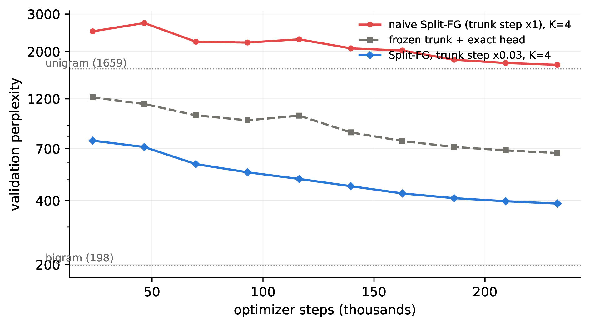
Figure 2: Frozen-trunk control, naive Split-FG (\(K{=}4\)), and \(\rho\)-scaled Split-FG on WikiText-103, same one-epoch cosine schedule (single seed). Naive trunk training tracks above the frozen control throughout; the \(\rho\)-scaled trunk drops below it from the first checkpoint and passes the frozen run’s final perplexity in about a quarter of the budget..
4.4.0.1 Results.
In this single-seed validation comparison, the same-architecture backpropagation reference (Adam, no weight decay, as for Split-FG) reaches perplexity \(149.6\); Split-FG with a reduced trunk step reaches \(386.7\) (Appendix 12.2). It performs better than the evaluated trainable no-global-backward baselines in this table. The comparison that most directly isolates the split is pure forward gradient at the same \(K{=}4\) and with the same learning-rate screening procedure (Appendix 12.1): it reaches \(2{,}885\), so removing the split, which estimates the head instead of solving it exactly, costs \(7.5\times\) at equal \(K\) (and \(104\times\) against the untuned \(K{=}1\) default). The training-free Hopfield/kNN-LM baseline holds \(6.6\times\) Split-FG’s memory. The count-based unigram/bigram references are fitted on the training tokens and evaluated identically; the interpolated bigram (\(198\)) still leads all evaluated trainable no-global-backward methods (Appendix 12.2). Split-FG trains in \(810.6\) MiB against \(1237.7\) MiB for backpropagation (\(\mathrm{MemSave}=34.5\%\), Eq. equation 21 ). The costs are a \(3.2\times\) step time and a \(2.6\times\) perplexity gap to backpropagation, which come from estimating the trunk with \(K\) scalar probes per step.
4.5 GPT Ablation Studies↩︎
We isolate each design choice by changing one component at a time from the main configuration (full tables in Appendices 12.3–12.6). Removing the trunk step scale costs \(4.5\times\) in perplexity, freezing the trunk costs \(1.7\times\), and dropping the split entirely costs \(7.5\times\) against a pure-FG baseline matched in tangent count and tuning (\(104\times\) against the untuned \(K{=}1\) default). These single-seed controls are consistent with the split removing a dominant noise source and the reduced step making the remaining trunk estimate usable. In the reported \(100\times\) grid of \(\rho\), every value beats the frozen control at both the screening and the full budget, with a broad minimum around \(\rho\in[0.03,0.1]\) (Table ¿tbl:tab:rho-ablation?; Appendix 12.4). Increasing \(K\) from \(1\) to \(8\) improves perplexity monotonically at constant peak memory (the \(K\) tangents run sequentially, each freeing its tape before the next) and sub-linear wall-clock cost (\(52\to187\) ms per step), making \(K\) a pure time–variance dial.
| Trunk step scale \(\rho\) | \(10\%\)-budget PPL | Full-budget PPL |
|---|---|---|
| \(0.003\) | \(716.1\) | \(622.7\) |
| \(0.01\) | \(681.8\) | \(514.9\) |
| \(0.03\) | \(623.3\) | \(386.7\) |
| \(0.1\) | \(541.9\) | \(365.0\) |
| \(0.3\) | \(677.9\) | \(633.1\) |
| Frozen control (\(K{=}0\)) | \(816.0\) | \(667.6\) |
Among optimizers (Appendix 12.5), the three adaptive methods cluster tightly (Muon \(382\), Adam \(387\), AdamW \(399\)) while SGD fails entirely (\(44{,}918\)): only a per-coordinate denominator can reconcile the \(O(1)\) head gradient with the \(O(P_{\mathrm{trunk}}/K)\) trunk estimate under one learning rate.
5 Discussion↩︎
5.0.0.1 Limitations.
Split-FG still trails backpropagation: on WikiText-103 it reaches perplexity \(387\), versus \(150\) with matched Adam and \(75.5\) with tuned AdamW, with gaps of \(27.7\) and \(30.4\) points on CIFAR-10 and CIFAR-100. Its variance also favors architectures with a large exact head; our flat-head image models make this trade-off by using a shallow feature extractor. Memory savings come at a substantial time cost (\(1.5\)–\(4.5\times\) slower steps for \(K{=}2\)–\(8\)), and activation checkpointing [23] or reversible architectures [24] remain stronger choices when memory is the only goal. Split-FG’s distinct property is eliminating reverse-mode passes through the trunk.This approach is especially valuable where a backward pass is unavailable, such as on the optical and analog accelerators motivating this work, as it obtains trunk gradients solely through forward perturb-and-measure techniques Our experiments are limited to a \(16\)M-parameter language model and vision backbones up to \(11\)M parameters on one 8 GB GPU; because variance scales as \(P_{\mathrm{trunk}}/K\), larger trunks remain the main open question. The GPT results are single-seed, use gradient clipping and a readout-only surrogate for tied embeddings (Appendices 9 and 12.7). Comparisons across \(K\) are additionally affected by separate annealing schedules.
5.0.0.2 A negative result: sizing the trunk to the probe budget.
We first tested whether reducing the forward-trained trunk to match the probe budget would help. This “light trunk” trains only positional embeddings, LayerNorm affines, and biases (\(46.6\)k parameters, roughly \(20\) probes per parameter), while freezing the trunk weight matrices. It only ties the frozen control (\(671.6\) vs.\(667.6\) perplexity), whereas the \(\rho\)-scaled full trunk reaches \(386.7\). The limiting factor is therefore step size, not probe count: with a reduced trunk step, even a severely under-determined trunk can learn. Here \(\rho\) is simply a per-group learning-rate multiplier [25]–[27]; the key point is that the noisy, estimated trunk gradient needs a much smaller step than the exact head gradient.
5.0.0.3 Future directions.
Two extensions stand out: conditioned tangents, which scale each tangent coordinate by a running gradient-magnitude estimate, reweighted to stay unbiased (preliminary runs: better sample efficiency, same plateau under full annealing) and broader head classes, e.g.a head-only backward pass for nonlinear heads or finite-difference head gradients for black-box heads.
6 Related Work↩︎
6.0.0.1 Forward gradients and zeroth-order training.
Forward-mode directional derivatives as unbiased gradient estimates were proposed by [4] and studied for representation learning by [28]; evolution strategies [5], [6] and zeroth-order fine-tuning [7] estimate the same object from function evaluations. All inherit variance that grows with the number of perturbed parameters. [15] reduce that dimension with layer-local losses at the price of a surrogate objective; Split-FG instead keeps the global loss and removes the head’s share of the dimension exactly, which is where most parameters live in our settings. Our frozen-trunk control asks a question this literature rarely does—whether the estimated component improves on not training it at all—and our answer (no, unless the update is rescaled) suggests such controls should be standard.
6.0.0.2 Local and biologically motivated learning.
Forward-Forward [13], predictive coding [10], [11], equilibrium propagation [8], and feedback alignment [14] avoid the backward pass with local objectives or fixed feedback, introducing bias; associative-memory readouts [19], [20] avoid training altogether. We compare against these families directly (Section 4).
6.0.0.3 Per-group step sizes.
Mechanically, our trunk step scale \(\rho\) is a per-group learning-rate multiplier—an axis long used by layer-wise adaptive methods [25], [29], discriminative fine-tuning howard2018universal?, and width-aware parameterisations [27]. We claim no novelty for the mechanism. The contribution is the diagnosis: with a mixed exact/estimated gradient, Adam-style normalisation equalises update magnitudes but not signal-to-noise, so the estimated group must be slowed by orders of magnitude (\(\rho\approx 0.03\) at \(P_{\mathrm{trunk}}{=}3.2\)M)—without which trunk training is worse than leaving the trunk frozen, a failure mode invisible unless the frozen control is run.
6.0.0.4 Memory-efficient exact-gradient training.
Activation checkpointing [23] and reversible architectures [24] reduce activation memory while keeping exact gradients, and on pure memory grounds they are strong alternatives to forward-mode training. Split-FG’s claim is different: it uses zero reverse-mode passes through the trunk, the regime relevant to hardware that cannot run a backward pass and to models of biological learning; its memory saving (Section 4) is a by-product, not the primary argument.
7 Variance Reduction Derivation↩︎
Let \(\theta=(\theta_{\mathrm{trunk}},\theta_{\mathrm{head}})\) and write \(F(\theta)\) for the full-batch training objective. At a fixed iterate, denote the exact gradients by \(g_{\mathrm{trunk}}=\nabla_{\theta_{\mathrm{trunk}}}F(\theta)\) and \(g_{\mathrm{head}}=\nabla_{\theta_{\mathrm{head}}}F(\theta)\). Split-FG draws \(K\) independent Gaussian tangent vectors \(v_k\sim\mathcal{N}(0,I_{P_{\mathrm{trunk}}})\) only in the trunk parameter space and uses \[\label{eq:split-estimator-analysis} \hat{g}_{\mathrm{trunk}} = \frac{1}{K}\sum_{k=1}^K \langle g_{\mathrm{trunk}},v_k\rangle v_k, \qquad \hat{g}_{\mathrm{head}} = g_{\mathrm{head}} .\tag{10}\] Unbiasedness follows from \(\mathbb{E}[v_kv_k^\top]=I\): \(\mathbb{E}[\langle g_{\mathrm{trunk}},v_k\rangle v_k] =g_{\mathrm{trunk}}\).
For a single tangent and a trunk coordinate \(i\), write \(\hat{g}_i=(\sum_j g_jv_j)v_i\). Since \(\mathbb{E}[v_jv_\ell v_i^2]=\delta_{j\ell} +2\delta_{ij}\delta_{i\ell}\) for Gaussian \(v\), \(\mathbb{E}[\hat{g}_i^2]=\lVert g_{\mathrm{trunk}}\rVert^2+2g_i^2\). Subtracting the squared mean \(g_i^2\) and averaging \(K\) independent samples gives \[\label{eq:split-coordinate-var} \mathrm{Var}\!\left[(\hat{g}_{\mathrm{trunk}})_i\right] = \frac{1}{K} \left( \lVert g_{\mathrm{trunk}}\rVert^2 + (g_{\mathrm{trunk}})_i^2 \right).\tag{11}\] Thus Split-FG replaces the pure forward-gradient dominant term \(\lVert\nabla F(\theta)\rVert^2\) by \(\lVert g_{\mathrm{trunk}}\rVert^2\) for each trunk coordinate; the head contribution is exact and contributes no estimator variance.
Summing over the \(P_{\mathrm{trunk}}\) trunk coordinates gives \[\begin{align} \label{eq:split-total-var} \mathbb{E}\!\left[\hat{g}\mid \theta\right] &= \nabla F(\theta),\\ \mathbb{E}\!\left[ \lVert \hat{g}-\nabla F(\theta)\rVert^2 \mid \theta \right] &= \frac{P_{\mathrm{trunk}}+1}{K} \lVert g_{\mathrm{trunk}}\rVert^2,\\ \mathbb{E}\!\left[ \lVert \hat{g}\rVert^2 \mid \theta \right] &= \lVert g_{\mathrm{head}}\rVert^2 + \left(1+\frac{P_{\mathrm{trunk}}+1}{K}\right) \lVert g_{\mathrm{trunk}}\rVert^2 . \end{align}\tag{12}\] For pure forward gradient over all \(P_{\mathrm{total}}\) parameters, the corresponding total variance is \(((P_{\mathrm{total}}+1)/K)\lVert\nabla F(\theta)\rVert^2\). Under roughly uniform gradient energy per coordinate, the dominant per-coordinate variance ratio becomes \(P_{\mathrm{trunk}}/P_{\mathrm{total}}\).
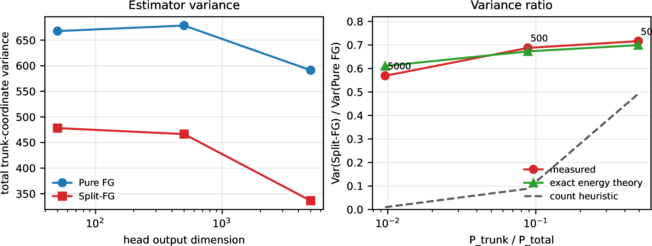
Figure 3: Controlled toy variance experiment (Section 4.1). Left: total empirical variance over trunk coordinates for pure forward gradient and Split-FG as the linear head grows. Right: the measured variance ratio tracks the gradient-energy prediction in Eq. equation 9 ; the parameter-count ratio is a useful heuristic only when gradient energy is approximately uniform across parameters..
| Classes | \(P_{\mathrm{total}}\) | \(P_{\mathrm{trunk}}/P_{\mathrm{total}}\) | Measured | Energy theory | Rel. error |
|---|---|---|---|---|---|
| 50 | 3250 | 0.4923 | 0.7162 | 0.6993 | 2.4% |
| 500 | 18100 | 0.0884 | 0.6875 | 0.6727 | 2.2% |
| 5000 | 166600 | 0.0096 | 0.5689 | 0.6104 | 6.8% |
8 Convergence Proofs↩︎
8.0.0.1 Formal statement (predictable-preconditioner Split-FG).
Let \(F\) denote the full-batch training objective. Assume that \(F\) is bounded below by \(F_\star\) and is \(L\)-smooth. Let \(\hat{g}_t\) be the Split-FG estimator at step \(t\), with an exact head component and a \(K\)-sample forward-gradient trunk component. Consider the diagonal-preconditioned update \[\label{eq:adam-style-update} \theta_{t+1}=\theta_t-\eta A_t \hat{g}_t, \qquad A_t=\mathrm{diag}(a_{t,1},\ldots,a_{t,P_{\mathrm{total}}}),\tag{13}\] where \(A_t\) is predictable given the history before drawing the current tangents and is uniformly bounded: \[\label{eq:adam-preconditioner-bounds} 0<a_{\min}\leq a_{t,i}\leq a_{\max}<\infty .\tag{14}\] Define the adaptive noise ratio \[\label{eq:adaptive-noise-ratio} R_t(A_t)= \frac{ \mathbb{E}_t[\lVert A_t\hat{g}_t\rVert^2] }{ \langle \nabla F(\theta_t),A_t\nabla F(\theta_t)\rangle }.\tag{15}\] When \(\nabla F(\theta_t)=0\), both numerator and denominator vanish for the full-batch estimator and we set \(R_t(A_t)=0\) by convention. If \(R_t(A_t)\leq R_{\max}\) almost surely and \(0<\eta\leq 1/(L R_{\max})\), then for any horizon \(T\), \[\label{eq:adam-style-convergence-weighted} \frac{1}{T}\sum_{t=0}^{T-1} \mathbb{E}\!\left[ \langle \nabla F(\theta_t),A_t\nabla F(\theta_t)\rangle \right] \leq \frac{2(F(\theta_0)-F_\star)}{\eta T}.\tag{16}\] Consequently, \[\label{eq:adam-style-convergence-euclidean} \frac{1}{T}\sum_{t=0}^{T-1} \mathbb{E}\!\left[\lVert\nabla F(\theta_t)\rVert^2\right] \leq \frac{2(F(\theta_0)-F_\star)}{\eta a_{\min}T}.\tag{17}\]
8.0.0.2 Predictable-preconditioner assumptions and weighted moment.
The theorem applies to a bounded diagonal preconditioner fixed before the current tangent draw, for example a deliberately lagged inverse-RMS preconditioner. It does not capture the exact Adam implementation in our experiments: both its first moment and its second-moment denominator are updated from the current stochastic estimate before the parameter step. Establishing a result for that optimizer requires a separate dependence analysis. Within the idealised algorithm, the trunk-specific step scale \(\rho\) of Appendix 12.2 multiplies the trunk entries of \(A_t\) by a constant and therefore preserves the theorem’s assumptions.
For a fixed diagonal preconditioner \(A_t\), Split-FG has the exact conditional weighted second moment \[\begin{align} \label{eq:adam-weighted-second-moment} \mathbb{E}_t\!\left[\lVert A_t\hat{g}_t\rVert^2\right] &= \lVert A_t g_{\mathrm{head},t}\rVert^2 +\sum_{i\in\mathrm{trunk}} a_{t,i}^2 \left[ \left(1+\frac{1}{K}\right)g_{t,i}^2 +\frac{1}{K}\lVert g_{\mathrm{trunk},t}\rVert^2 \right]. \end{align}\tag{18}\] This identity explains the possible role of predictable inverse-RMS scaling: noisy trunk coordinates with large past running second moment can acquire smaller \(a_{t,i}\), so their contribution to the smoothness penalty is reduced quadratically, while the exact head coordinates carry no forward-gradient variance term. A coarse worst-case bound is \(R_{\max}\leq (a_{\max}^2/a_{\min})(1+(P_{\mathrm{trunk}}+1)/K)\), recovering the unpreconditioned Split-FG scaling up to conditioning of the diagonal preconditioner.
If an implementation shares a parameter between the trunk computation and the exact head, the theorem applies to the strict estimator that includes both contributions (the include_tied variant). It does not cover the readout-only
surrogate used in our GPT runs: there the stop-gradient copy of the lookup role is redefined at every iterate, so no fixed \(L\)-smooth, lower-bounded objective telescopes in the descent argument; the guarantee applies to
the untied parameters, and the tied table’s update is a heuristic we disclose (Appendix 12.7).
8.0.0.3 Proof of the predictable-preconditioner theorem.
For a trunk coordinate \(i\), Eq. equation 11 gives \[\mathbb{E}_t[\hat{g}_{t,i}^2] = \left(1+\frac{1}{K}\right)g_{t,i}^2 +\frac{1}{K}\lVert g_{\mathrm{trunk},t}\rVert^2 ,\] where \(\mathbb{E}_t[\cdot]\) conditions on the current iterate and all previous randomness. For head coordinates, Split-FG is exact: \(\hat{g}_{t,i}=g_{t,i}\). Since \(A_t\) is fixed under \(\mathbb{E}_t[\cdot]\), multiplying by \(a_{t,i}^2\) and summing over coordinates proves the weighted second-moment identity in Eq. equation 18 .
By \(L\)-smoothness and the update \(\theta_{t+1}=\theta_t-\eta A_t\hat{g}_t\), \[\begin{align} \mathbb{E}_t[F(\theta_{t+1})] &\leq F(\theta_t) -\eta \left\langle \nabla F(\theta_t),A_t\mathbb{E}_t[\hat{g}_t] \right\rangle +\frac{L\eta^2}{2} \mathbb{E}_t[\lVert A_t\hat{g}_t\rVert^2]\\ &= F(\theta_t) -\eta \langle \nabla F(\theta_t),A_t\nabla F(\theta_t)\rangle +\frac{L\eta^2}{2} \mathbb{E}_t[\lVert A_t\hat{g}_t\rVert^2]\\ &\leq F(\theta_t) -\eta \left(1-\frac{L\eta R_{\max}}{2}\right) \langle \nabla F(\theta_t),A_t\nabla F(\theta_t)\rangle\\ &\leq F(\theta_t) -\frac{\eta}{2} \langle \nabla F(\theta_t),A_t\nabla F(\theta_t)\rangle . \end{align}\] The second line uses Split-FG unbiasedness, and the third uses the definition of \(R_t(A_t)\) together with \(R_t(A_t)\leq R_{\max}\). Taking total expectation, summing from \(t=0\) to \(T-1\), and using \(F(\theta_T)\geq F_\star\) gives Eq. equation 16 . Finally, \(A_t\succeq a_{\min}I\) implies \(\langle\nabla F(\theta_t),A_t\nabla F(\theta_t)\rangle \geq a_{\min}\lVert\nabla F(\theta_t)\rVert^2\), yielding Eq. equation 17 .
8.0.0.4 SGD baseline theorem.
For comparison, the unpreconditioned Split-FG update also converges under the standard nonconvex stochastic-gradient argument. Assume \(F\) is differentiable, bounded below by \(F_\star\), and \(L\)-smooth. Run the SGD version of Split-FG, \[\theta_{t+1}=\theta_t-\eta\hat{g}_t,\] where the head gradient is exact and the trunk estimator is Eq. equation 10 . If \[\label{eq:split-sgd-stepsize} 0<\eta\leq \frac{1}{ L\left(1+(P_{\mathrm{trunk}}+1)/K\right)},\tag{19}\] then for any horizon \(T\), \[\label{eq:split-sgd-convergence} \frac{1}{T}\sum_{t=0}^{T-1} \mathbb{E}\!\left[\lVert\nabla F(\theta_t)\rVert^2\right] \leq \frac{2\left(F(\theta_0)-F_\star\right)}{\eta T}.\tag{20}\] Taking the largest allowed step size yields \[\min_{0\leq t<T} \mathbb{E}\!\left[\lVert\nabla F(\theta_t)\rVert^2\right] \leq \frac{ 2L\left(1+(P_{\mathrm{trunk}}+1)/K\right) \left(F(\theta_0)-F_\star\right) }{T}.\] Thus full-batch Split-FG reaches a first-order stationary point at the standard nonconvex stochastic-gradient rate, with the forward-gradient penalty depending on \(P_{\mathrm{trunk}}\) rather than \(P_{\mathrm{total}}\).
8.0.0.5 Proof of the SGD baseline.
By \(L\)-smoothness and the update rule, \[\begin{align} \mathbb{E}_t[F(\theta_{t+1})] &\leq F(\theta_t) -\eta \left\langle \nabla F(\theta_t),\mathbb{E}_t[\hat{g}_t] \right\rangle +\frac{L\eta^2}{2}\mathbb{E}_t[\lVert\hat{g}_t\rVert^2]\\ &= F(\theta_t) -\eta\lVert\nabla F(\theta_t)\rVert^2 +\frac{L\eta^2}{2} \left[ \lVert g_{\mathrm{head},t}\rVert^2 + \left(1+\frac{P_{\mathrm{trunk}}+1}{K}\right) \lVert g_{\mathrm{trunk},t}\rVert^2 \right]\\ &\leq F(\theta_t) -\eta \left[ 1-\frac{L\eta}{2} \left(1+\frac{P_{\mathrm{trunk}}+1}{K}\right) \right] \lVert\nabla F(\theta_t)\rVert^2\\ &\leq F(\theta_t) -\frac{\eta}{2} \lVert\nabla F(\theta_t)\rVert^2 . \end{align}\] The second line uses unbiasedness and the second-moment identity from Eq. equation 12 ; the final line uses Eq. equation 19 . Taking total expectation, summing over \(t=0,\ldots,T-1\), and using \(F(\theta_T)\geq F_\star\) proves Eq. equation 20 .
8.0.0.6 Minibatches.
With minibatches, the same argument applies after adding the usual data-noise term. If the combined estimator remains unbiased for \(\nabla F(\theta_t)\) and has conditional second moment at most \(\left(1+(P_{\mathrm{trunk}}+1)/K\right)\lVert\nabla F(\theta_t)\rVert^2 +\sigma_{\mathrm{data}}^2\), then the SGD bound becomes \[\frac{1}{T}\sum_{t=0}^{T-1} \mathbb{E}\!\left[\lVert\nabla F(\theta_t)\rVert^2\right] \leq \frac{2\left(F(\theta_0)-F_\star\right)}{\eta T} +L\eta\sigma_{\mathrm{data}}^2.\] The additional term is the standard minibatch stochastic-gradient term; the structural Split-FG contribution still scales with \(P_{\mathrm{trunk}}/K\).
9 General Experimental Protocol↩︎
9.0.0.1 Backpropagation-reference protocol.
The tabular and GPT comparisons use the same dataset, preprocessing, architecture, loss function, data exposure, and optimizer family for Split-FG and their backpropagation references. For language models this means the same number of training tokens and optimizer updates. The image headline table is a system comparison: Split-FG uses a light-trunk/flat-head architecture while the backpropagation, Pure-FG, and ES references use standard full ResNets and the other baselines use their native architectures. The image appendix therefore reports the architecture-matched flat-head estimator ablation separately. Wall-clock time is reported as an outcome, not a matching criterion.
9.0.0.2 Memory metric.
For each large experiment we report peak GPU memory and the relative difference of Split-FG from its stated backpropagation reference: \[\label{eq:memory-saving} \mathrm{MemSave} = 1 - \frac{ M_{\mathrm{peak}}(\mathrm{Split\text{-}FG}) }{ M_{\mathrm{peak}}(\mathrm{Backprop}) } .\tag{21}\] We also report held-out-fold, development, or validation performance as labelled and step time; the ablation tables additionally report JVPs per step, and every Split-FG run uses zero reverse-mode passes through the trunk.
9.0.0.3 Gradient clipping.
Every run in the paper—backpropagation included—applies global-norm clipping at \(1.0\) to the assembled gradient estimate (all parameter groups jointly) before the optimizer step. For high-variance estimates whose norm exceeds the threshold, clipping rescales the whole update and thereby introduces a bias not covered by the analysis of Section 3, which treats the unclipped estimator; the protocol is uniform across methods, so comparisons within each table share it.
9.0.0.4 Backprop-free baselines.
The Forward-Forward algorithm [13] trains each layer with a local goodness objective on positive and negative (label-overlaid) inputs and is defined for classification only; it therefore appears in the tabular-classification and image experiments but not in regression or language modelling. Predictive coding [10], [11] settles layer-wise latent variables to minimise local prediction errors and then applies local Hebbian weight updates; it applies to both classification and regression and, in the small-step-size limit, approximates the backpropagation gradient using only local computation. The modern Hopfield associative-memory baseline [19] performs a training-free softmax retrieval over a frozen trunk, storing \((\text{feature},\text{target})\) pairs and answering queries by \(w=\mathrm{softmax}(\beta\, q K^\top)\), \(\hat{y}=wV\); for language modelling this reduces to per-token nearest-neighbour recall in the spirit of kNN-LM [20]. All three baselines use zero JVPs and zero trunk backward passes, isolating how much of each task is solvable by local goodness training, local error settling, or associative recall over a random representation.
10 Tabular Data↩︎
10.1 Tabular Dataset Details↩︎
Table ¿tbl:tab:tabular-datasets? summarizes the eight default tabular datasets used in the experiments of Section 4.2. They are standard public benchmarks obtained from OpenML (with Kaggle origins for Otto Group Products and Diamond), chosen to cover binary classification, multiclass classification, and regression across a range of feature counts and dataset sizes. Following the preprocessing in our loader, numeric features are standardised to zero mean and unit variance and categorical features are integer-encoded. We use \(5\)-fold cross-validation for all datasets and methods; each fold trains under the fixed \(300\)-step budget of Appendix 10.2.
| Dataset | Domain | Task | #Samples | #Feat. | #Cls. | Source |
|---|---|---|---|---|---|---|
| Adult | Census income | Binary classification | \(48{,}842\) | \(14\) | \(2\) | OpenML |
| Higgs Small | Particle physics | Binary classification | \(98{,}050\) | \(28\) | \(2\) | OpenML |
| Otto Group Products | E-commerce | Multiclass classification | \(61{,}878\) | \(93\) | \(9\) | Kaggle/OpenML |
| Covertype | Forest cartography | Multiclass classification | \(581{,}012\) | \(54\) | \(7\) | OpenML |
| California Housing | Housing prices | Regression | \(20{,}640\) | \(8\) | – | OpenML |
| House 16H | Housing prices | Regression | \(22{,}784\) | \(16\) | – | OpenML |
| Diamond | Diamond prices | Regression | \(53{,}940\) | \(9\) | – | Kaggle/OpenML |
| Black Friday | Retail purchases | Regression | \(166{,}821\) | \(9\) | – | OpenML |
10.2 Tabular Experimental Protocol↩︎
10.2.0.1 Metrics.
For the classification datasets we report held-out-fold accuracy (%, higher is better); for the regression datasets we report held-out-fold RMSE (lower is better) on the standardised targets. Because the loader standardises regression targets using training-fold statistics, RMSE is expressed in units of target standard deviations. Classification is trained with cross-entropy and regression with MSE.
10.2.0.2 Methods.
Each dataset is run with matched backpropagation, pure forward gradient (Pure FG), antithetic evolution strategies (ES), and the no-global-backward baselines Forward-Forward (FF), predictive coding (PC), and the Hopfield associative-memory readout (Hop.), against Split-FG. FF applies only to classification (“–” for regression); PC and Hopfield apply to both. Every Split-FG run is paired with the matched backpropagation version of the same TabM-style model (Appendix 10.3).
10.2.0.3 Training budget.
Every method uses a fixed budget of \(300\) optimiser steps at batch size \(256\), run once per cross-validation fold with seed \(0\); the \(\pm\) values in Table ¿tbl:tab:tabular-main? are standard deviations over the \(5\) folds, not over seeds. The effective number of epochs is \(\mathrm{steps}\times\mathrm{batch}/N_{\mathrm{train}}\) and so varies with dataset size (reported in Table ¿tbl:tab:tabular-memory?): under this controlled budget the largest datasets (Covertype, Black Friday) see well under one epoch.
10.2.0.4 Memory measurement.
Table ¿tbl:tab:tabular-memory? reports peak GPU memory via torch.cuda.max_memory_allocated, reset at the start of training, and \(\mathrm{MemSave}=1-M_{\mathrm{peak}}(\text{Split-FG})/
M_{\mathrm{peak}}(\text{Backprop})\) (Eq. equation 21 ). Both methods keep the full dataset resident on-device, so the peak includes the data tensors; this dilutes the activation-graph saving on the largest
datasets, which is why the relative saving is largest for the smallest dataset (California Housing, \(24.1\%\)) and smallest for the largest (Black Friday, \(4.3\%\)). All runs use a single
NVIDIA RTX 4070 laptop GPU.
| Dataset | Loss | Epochs | Backprop mem.(MiB) | Split-FG mem.(MiB) | MemSave |
|---|---|---|---|---|---|
| Adult | CE | \(2.3\) | \(144.4\) | \(126.0\) | \(12.7\%\) |
| Covertype | CE | \(0.2\) | \(309.8\) | \(291.1\) | \(6.0\%\) |
| California Housing | MSE | \(5.3\) | \(76.0\) | \(57.7\) | \(24.1\%\) |
| Diamond | MSE | \(2.0\) | \(156.9\) | \(138.6\) | \(11.7\%\) |
| Black Friday | MSE | \(0.7\) | \(425.2\) | \(406.9\) | \(4.3\%\) |
10.3 Tabular Model Architecture↩︎
All tabular experiments (Table ¿tbl:tab:tabular-main?) use the same TabM-style parameter-efficient MLP ensemble [21]. We reserve \(K\) for the number of forward-gradient tangent samples and write the TabM ensemble count as \(k_{\mathrm{ens}}\). A single shared MLP is evaluated by \(k_{\mathrm{ens}}\) ensemble members that differ only through BatchEnsemble rank-1 multiplicative adapters: at each layer member \(i\) computes \(y_i = \big((x_i \odot r_i)\,W^\top\big)\odot s_i + b\), with a shared weight \(W\) and bias \(b\) and per-member vectors \(r_i, s_i\) (initialised near \(1\) to break symmetry). The per-member representations are averaged before a single shared linear head; because averaging is linear, this keeps the head a single linear layer, so the trunk/head split admits the closed-form CE/MSE head gradient of Eq. equation 7 . For the MSE case, with \(\hat{y}=hW_{\mathrm{head}}^\top+b\) and \(\mathcal{L}=(2N)^{-1}\lVert \hat{y}-y\rVert^2\), the closed forms are \(\partial\mathcal{L}/\partial W_{\mathrm{head}} = r^\top h\), \(\partial\mathcal{L}/\partial b=\sum_n r_n\), and \(\partial\mathcal{L}/\partial h=rW_{\mathrm{head}}\), where \(r=(\hat{y}-y)/N\). The trunk (input broadcast, the \(n_{\mathrm{layers}}\) BatchEnsemble layers, and the member average) is the nonlinear part estimated by forward-gradient JVPs; the linear head is estimated exactly. Table ¿tbl:tab:tabular-arch? lists the structure.
Default hyperparameters: hidden width \(d_h=128\), \(n_{\mathrm{layers}}=2\) shared layers, \(k_{\mathrm{ens}}=8\) ensemble members, \(K=8\) forward-gradient tangent samples, the Adam optimizer at learning rate \(3\times10^{-3}\), batch size \(256\), trained for \(300\) steps. Here \(n\) denotes the number of input features and \(C\) the number of outputs (\(C\) classes for classification, \(C=1\) for regression), both dataset-dependent (Table ¿tbl:tab:tabular-datasets?); \(B\) is the batch size.
| Layer | Operation | Output shape | Description |
|---|---|---|---|
| Input | Standardised features | \((B, n)\) | Numerical features standardised; categoricals integer-encoded and appended. |
| Broadcast | Replicate to \(k_{\mathrm{ens}}\) members | \((B, k_{\mathrm{ens}}, n)\) | Shared input copied to all \(k_{\mathrm{ens}}\) ensemble members. |
| 1 | BatchEnsemble Linear \(+\) ReLU | \((B, k_{\mathrm{ens}}, d_h)\) | Shared \(W_1\in\mathbb{R}^{d_h\times n}\), bias; per-member rank-1 scales \(r_1,s_1\). |
| 2 | BatchEnsemble Linear \(+\) ReLU | \((B, k_{\mathrm{ens}}, d_h)\) | Shared \(W_2\in\mathbb{R}^{d_h\times d_h}\), bias; per-member rank-1 scales \(r_2,s_2\). |
| Mean | Average over members | \((B, d_h)\) | \(\bar h=\tfrac{1}{k_{\mathrm{ens}}}\sum_{i=1}^{k_{\mathrm{ens}}} h_i\); linearises the head. |
| — trunk / head split — | |||
| Head | Linear | \((B, C)\) | Shared \(W_{\mathrm{head}}\in\mathbb{R}^{C\times d_h}\), bias; averaged logits (cls.) / prediction (reg.). |
| Output | CE / MSE loss | scalar | Cross-entropy (classification) or \(\tfrac{1}{2}\) MSE (regression). |
11 Image Dataset Details↩︎
Table ¿tbl:tab:image-datasets? summarizes the image-classification benchmarks used in Section 4.3. CIFAR-10 and CIFAR-100 [30] are standard \(32\times32\) natural-image datasets with a fixed \(50{,}000\)/\(10{,}000\) train/test split; Following the preprocessing in our loader, images are standardised per channel; at training time CIFAR uses standard augmentation (reflection padding with a random \(32\times32\) crop and a random horizontal flip). Unlike the smaller tabular datasets, which use \(5\)-fold cross-validation, the current image artifacts use the fixed official train/test split. Because the test split was inspected during method development and evaluation samples random batches from it, we label these values development evaluation rather than final held-out test results (Appendix 11.1).
| Dataset | Domain | Task | #Samples | Res. | #Cls. | Source |
|---|---|---|---|---|---|---|
| CIFAR-10 | Natural images | Multiclass classification | \(60{,}000\) | \(32\times32\) | \(10\) | [30] |
| CIFAR-100 | Natural images | Multiclass classification | \(60{,}000\) | \(32\times32\) | \(100\) | [30] |
11.1 Image Experimental Protocol↩︎
11.1.0.1 Metrics.
The backpropagation, Pure-FG, ES, and Split-FG artifacts report top-1 accuracy (%, higher is better) by sampling \(50\) random batches of size \(128\) from the official CIFAR test split; the FF, PC, and Hopfield runners evaluate all \(10{,}000\) examples. Thus the former are Monte Carlo estimates, not deterministic full-test passes. Moreover, that split was inspected during method development, so Table ¿tbl:tab:image-main? is labelled development evaluation. All trainable models use cross-entropy. CIFAR-10 and CIFAR-100 entries are reported as mean \(\pm\) standard deviation over five seeds.
11.1.0.2 Methods.
Each dataset is run with a standard-backbone backpropagation reference, pure forward gradient (Pure FG), antithetic evolution strategies (ES), and the no-global-backward baselines Forward-Forward (FF), predictive coding (PC), and the Hopfield associative-memory readout (Hop.), against Split-FG. Pure FG and ES use the standard ResNet-20 with all parameters estimated: Pure FG by a single full-network JVP (variance \(\propto P_{\mathrm{total}}\)) and ES by a two-point zeroth-order finite difference. FF and PC are self-contained two-hidden-layer MLPs on the flattened image trained without any global backward pass. More specifically, FF greedily optimises a layer-local “goodness” objective with the label overlaid on the input, and PC settles per-layer latents and updates weights by a local Hebbian rule. Hopfield is training-free: a frozen random trunk maps inputs to features and a modern-Hopfield/\(k\)NN memory answers queries by softmax retrieval over stored (feature, target) pairs. Split-FG uses the heavy-head/light-trunk flat-head restructuring (Appendix 11.2). The standard-ResNet backpropagation row is a same-data-exposure reference, not an architecture-matched estimator control; the latter is reported in Appendix 11.3.
11.1.0.3 Training budget.
CIFAR-10 uses \(23{,}437\) steps at batch size \(128\) (\(\approx60\) epochs) for every reported method. CIFAR-100 uses that budget only for backpropagation and Split-FG; Pure FG uses \(2{,}000\) steps (\(5.12\) epochs), ES \(400\) (\(1.02\) epochs), FF and PC \(3{,}000\) (\(7.68\) epochs), and Hopfield is training-free. These early-stopped rows diagnose failure at their stated budgets but are not comparable as a matched-budget ranking. Trainable image methods use Adam at learning rate \(1\times10^{-3}\) and standard augmentation; the 60-epoch runs use a cosine schedule. CIFAR-10 uses \(200\) warmup steps and no weight decay; CIFAR-100 uses \(300\) warmup steps and weight decay \(5\times10^{-4}\) where applicable (Appendix 11.2). The forward-gradient methods use \(K=4\) tangent samples. The \(15.4\)-epoch (\(6000\)-step) protocol is retained only for the flat-head estimator ablation in Appendix 11.3.
11.1.0.4 Memory measurement.
Table ¿tbl:tab:image-memory? reports peak GPU memory via torch.cuda.max_memory_allocated, reset at the start of training, and \(\mathrm{MemSave}=1-M_{\mathrm{peak}}(\text{Split-FG})/
M_{\mathrm{peak}}(\text{Backprop})\) (Eq. equation 21 ). Unlike the small tabular and linear models, a convolutional trunk carries large activation maps, and forward mode carries a tangent copy of the trunk
activations; because the \(K\) tangents are evaluated sequentially, peak memory does not grow with \(K\). The comparison therefore spans architectures: the flat-head Split-FG model versus
the full ResNet-20 backprop reference. For reference, carrying full-network tangents on the standard CIFAR-10 backbone (pure FG at \(K{=}4\), memory-identical to the naive full-trunk split) peaks at \(2668\) MiB—the blow-up quoted in Section 4.3.
| Dataset | BP backbone | Epochs | Backprop mem.(MiB) | Split-FG mem.(MiB) | RefDiff | Top-1 gap |
|---|---|---|---|---|---|---|
| CIFAR-10 | ResNet-20 | \(60\) | \(1520\) | \(1282\) | \(+15.6\%\) | \(-27.7\) |
| CIFAR-100 | ResNet-18 | \(60\) | \(3402\) | \(3117\) | \(+8.4\%\) | \(-30.4_{\pm1.4}\) |
11.2 Image Model Architecture↩︎
11.2.0.1 Backprop, Pure FG and ES backbones.
CIFAR-10 uses a standard CIFAR ResNet-20 [31]: a \(3\times3\) stem (\(3\to16\))
followed by three stages of three BasicBlocks at widths \(16/32/64\) (spatial \(32/16/8\)), global average pooling and a linear head—\(\approx\!272\)k
parameters. The harder \(100\)-class CIFAR-100 uses the larger ResNet-18: a \(3\times3\) stem (\(3\to64\), the CIFAR adaptation with no max-pool) and four
stages of two BasicBlocks at widths \(64/128/256/512\) (spatial \(32/16/8/4\)), global average pooling and a linear head—\(\approx\!11.2\)M parameters. Both
replace BatchNorm with GroupNorm, so the trunk is a pure function of its parameters and is differentiable under torch.func.jvp in .eval() mode.
11.2.0.2 Split-FG flat head.
Split-FG keeps only the stem and the first BasicBlock as the forward-mode trunk and flattens its feature map into a large two-layer linear head \(W_2 W_1\) trained by the exact closed-form gradient (no activation, no backward pass through the trunk; Table ¿tbl:tab:image-arch?). The first block inherits the backbone’s first-stage width, so the trunk is \(5{,}136\) parameters (flattened feature \(16\times32\times32{=}16{,}384\), \(H{=}64\)) for the ResNet-20 on CIFAR-10, and \(75{,}840\) parameters (flattened \(64\times32\times32{=}65{,}536\), \(H{=}128\)) for the ResNet-18 on CIFAR-100. In both, the trunk is under \(1\%\) of the head’s parameters, and \(H\) exceeds the class count so the factored head stays full rank.
11.2.0.3 FF and PC.
Forward-Forward and predictive coding are MLP-based local-learning rules and cannot use a convolutional backbone; we run them on a parameter-matched MLP over the flattened image (\(3072\to2000\to2000\), \(\approx\!10\)M parameters, comparable to the ResNet-18).
11.2.0.4 Hyperparameters.
GroupNorm with \(8\) groups, the Adam optimizer, and \(K{=}4\) forward-gradient tangents throughout. CIFAR-10: learning rate \(1\times10^{-3}\), cosine schedule (\(200\) warmup), batch \(128\), \(60\) epochs (the \(6000\)-step / \(15.4\)-epoch budget is used only for the ablation of Appendix 11.3). CIFAR-100 backpropagation and Split-FG: learning rate \(1\times10^{-3}\), weight decay \(5\times10^{-4}\), cosine schedule (\(300\) warmup), batch \(128\), \(60\) epochs; the other methods use the shorter budgets stated in Appendix 11.1. Here \(C\) is the number of classes and \(B\) the batch size.
| Layer | Operation | Output shape | Description |
|---|---|---|---|
| Input | Image | \((B,3,32,32)\) | Per-channel standardised; train-time reflect-crop \(+\) horizontal flip. |
| Stem | \(3\times3\) Conv, GN, ReLU | \((B,w,32,32)\) | \(3\to w\) channels, stride \(1\), padding \(1\); GroupNorm (\(8\) groups). |
| Block 1 | BasicBlock | \((B,w,32,32)\) | Two \(3\times3\) convs \(w\to w\) (Conv-GN-ReLU, Conv-GN) with identity shortcut, then ReLU. |
| Flatten | Reshape | \((B,1024w)\) | The \(w\times32\times32\) feature map flattened (\(1024w\)). |
| — trunk / head split — | |||
| Head 1 | Linear | \((B, H)\) | Shared \(W_1\in\mathbb{R}^{H\times 1024w}\), bias; no activation. |
| Head 2 | Linear | \((B, C)\) | Shared \(W_2\in\mathbb{R}^{C\times H}\), bias; logits \(=W_2(W_1 h)+b\) (factored linear). |
| Output | CE loss | scalar | Cross-entropy over \(C\) classes. |
11.3 Flat-head Estimator Ablation↩︎
To separate the contribution of Split-FG’s exact head from the choice of architecture, Table ¿tbl:tab:image-ablation? runs every estimator on the same flat-head network (CIFAR-10, the \(15.4\)-epoch/\(6000\)-step budget, which is why its Split-FG entry sits below the \(60\)-epoch \(60.5\%\) of Table ¿tbl:tab:image-main?). Pure FG and ES estimate all \(\approx\!1.05\)M parameters — the two-layer linear head alone is \(99.5\%\) of them — whereas Split-FG estimates only the \(5{,}136\)-parameter trunk and computes the head gradient exactly. Treating the head exactly is worth \(+34\) points over forward-estimating it (\(56.9\) vs \(22.6\)): on a fixed network, the variance of estimating a million-parameter head (\(\propto P_{\mathrm{total}}\)) is precisely what the split removes, while backprop on the same net (\(70.7\%\)) bounds the architecture. The table also includes Split-FG with a single exact linear head (\(54.4_{\pm1.5}\)): the factored two-layer head of Section 4.3 improves on it by \(+2.5\) points (paired \(t(4)=6.93\), \(p<0.01\)), the deep-linear over-parameterisation effect cited in the main text. This is the architecture-matched comparison underlying the Split-FG column of Table ¿tbl:tab:image-main?.
| Estimator on the flat-head net | Params estimated | Top-1 (%) |
|---|---|---|
| Backprop (exact reverse mode) | — (exact) | \(70.7_{\pm0.3}\) |
| Split-FG (exact \(2\)-layer linear head) | trunk only (\(5{,}136\)) | \(\mathbf{56.9_{\pm1.2}}\) |
| Split-FG (exact single linear head) | trunk only (\(5{,}136\)) | \(54.4_{\pm1.5}\) |
| Pure FG (forward gradient) | all (\(1.05\)M) | \(22.6_{\pm1.4}\) |
| ES (antithetic, zeroth-order) | all (\(1.05\)M) | \(21.7_{\pm1.9}\) |
12 GPT-Style Language-Modelling Details↩︎
Table ¿tbl:tab:gpt-datasets? summarizes the language-modelling dataset used in Section 4.4. We use WikiText-103 raw [32], tokenized with the GPT-2 byte-pair encoding [33] (\(50{,}257\) tokens). In summary, we have \(119{,}085{,}169\) train tokens and \(249{,}750\) validation tokens.
| Dataset | Split | Tokenizer | Tokens | Eval tokens | Source |
|---|---|---|---|---|---|
| WikiText-103 | Train | GPT-2 BPE | \(119{,}085{,}169\) | – | wikitext-103-raw-v1 |
| WikiText-103 | Val. | GPT-2 BPE | \(249{,}750\) | \(249{,}728\) | wikitext-103-raw-v1 |
12.1 GPT Experimental Protocol↩︎
12.1.0.1 Metrics.
We report validation negative log-likelihood (NLL) and perplexity, where \(\mathrm{PPL}=\exp(\mathrm{NLL})\), together with wall-clock time, mean step time, peak GPU memory, number of JVPs per step, and backward trunk passes. Validation is a full pass over the validation token stream using non-overlapping windows; no validation minibatches are sampled for the reported main run.
12.1.0.2 Methods.
The main GPT comparison uses same-architecture, same-token-exposure backpropagation with Adam and no weight decay (the recipe used by Split-FG; an AdamW variant with decoupled weight decay \(0.01\) reaches perplexity \(75.5\) and is noted in the caption of Table ¿tbl:tab:main-lm?), pure forward gradient with Adam, pure forward gradient with SGD, antithetic ES with Adam, the Hopfield associative-memory/kNN-LM baseline, and Split-FG with Adam. Forward-Forward is omitted because it is not defined for next-token language modelling; predictive coding and equilibrium propagation are omitted because our implementations of those baselines do not extend to next-token language modelling. The Hopfield/kNN-LM row is training-free: a frozen random GPT trunk maps training windows to features and validation queries retrieve next-token distributions by softmax \(k\)NN over the stored features. On the 8GB run we cap the store at \(4096\) train windows and evaluate all validation windows; its reported time entry in Table ¿tbl:tab:main-lm? is one full retrieval-evaluation pass rather than a training-step time.
12.1.0.3 Training budget.
All GPT runs use the small8 GPT configuration in Table ¿tbl:tab:gpt-arch?: \(L=4\) layers, \(d_{\mathrm{model}}=256\), \(4\)
attention heads, \(d_{\mathrm{ff}}=1024\), sequence length \(T=128\), and batch size \(4\). Training uses deterministic non-overlapping windows over the full
tokenized WikiText-103 train split. This gives \(930{,}352\) train windows and \(232{,}588\) optimizer steps for one epoch. All trainable methods use the same number of optimizer steps and
the same token exposure. The optimizer schedule is cosine decay with \(100\) warmup steps. The default learning rate is \(1.5\times10^{-3}\) for Adam/AdamW methods and \(5\times10^{-4}\) for the SGD forward-gradient baseline. The main table reports Split-FG at \(K{=}4\) with the reduced trunk step (\(\rho=0.03\), Appendix 12.2) alongside the naive-step run at the same \(K\); the frozen-trunk control uses \(K{=}0\) (head-only), and the \(K\)-ablation table reports the sweep with the same reduced trunk step. Mechanically, the trunk step scale multiplies the Adam update of every trunk parameter by \(\rho\) while the head
parameters keep the base learning rate; it changes neither the estimator nor the memory or step time.
12.1.0.4 Gradient-energy measurement.
The gradient-energy ratio quoted in Section 2.2 is measured at initialisation (seed \(0\), the same initialisation as every small8 run) by computing exact backpropagation
gradients on \(16\) sequential non-overlapping WikiText-103 training minibatches (\(T{=}128\), \(B{=}4\)) and averaging the per-batch ratio \(\lVert\nabla_{\theta_{\mathrm{trunk}}}\mathcal{L}\rVert^2/\lVert\nabla_{\theta}\mathcal{L}\rVert^2\) under the same exclude_tied trunk/head partition used for training; the measurement script is included in the
supplementary material. The ratio evolves over training; we report the initialisation value.
12.1.0.5 Pure-FG baseline tuning.
The \(K{=}4\) pure-FG row of Table ¿tbl:tab:main-lm? is tuned by the same screening protocol as \(\rho\) (fully annealed runs at the \(10\%\)-epoch budget of \(23{,}258\) steps, one full epoch at the argmin), applied to a six-point learning-rate grid. Screening validation perplexities: \(3\times10^{-3}\): \(21{,}319\); \(1.5\times10^{-3}\): \(8{,}026\); \(4.5\times10^{-4}\): \(4{,}544\) (argmin); \(1.5\times10^{-4}\): \(6{,}111\); \(4.5\times10^{-5}\): \(16{,}510\); \(1.5\times10^{-5}\): \(32{,}543\). The full-epoch run at the argmin reaches \(2{,}885\) (the value in Table ¿tbl:tab:main-lm?). The grid is over the global learning rate because pure FG has no exact/estimated group split; it spans \(200\times\), comparable to the \(100\times\) span of the five-point \(\rho\) grid in Table ¿tbl:tab:rho-ablation?.
12.2 Frozen-Trunk Control and the Trunk Step Scale↩︎
Because Split-FG’s head is exact, any comparison against other estimators leaves one question open: does the forward-gradient trunk training contribute, or is the exact head over random features doing all the work? We answer it with the cheapest possible control: freeze the trunk at its random initialisation and train only the head with the exact gradient, under an identical budget and schedule. Table ¿tbl:tab:main-lm? in the main text gathers the outcome, including two count-based references fitted on the training tokens and evaluated under the same windowed protocol (a unigram model, \(1659\), and an interpolated bigram model, \(198\)); Figure 2 (main text) shows the trajectories.
12.2.0.1 Naive trunk training hurts at this scale.
The frozen control reaches perplexity \(667.6\): a random causal transformer is already a strong feature extractor, and the exact head reads substantial structure off it (well below the unigram reference). Naive Split-FG, by contrast, converges at \(1733.4\) at \(K{=}4\) (the run shown in Figure 2; even \(K{=}8\) only reaches \(1656.7\))—above the frozen control and near the unigram level. Training the trunk with the naive step destroys more than it learns.
12.2.0.2 Diagnosis: a noise-blind step size.
The trunk estimate is unbiased, but its per-coordinate signal-to-noise ratio is \({\sim}1/P_{\mathrm{trunk}}\) (Eq. equation 5 ), and one epoch supplies only \(\mathrm{steps}\times K/P_{\mathrm{trunk}}\approx0.3\) scalar probes per trunk parameter—the trunk is under-determined within the budget. Adam is blind to this: its second-moment normalisation drives every coordinate at approximately full step length, whether its gradient estimate is signal or noise. On this account, the trunk executes a near-full-speed random walk away from its good random initialisation while the exact head continuously re-fits a drifting, degrading representation. We emphasise that the controls are consistent with this mechanism rather than a proof of it (we do not trace trunk displacement directly), but under it the failure is due to the step size rather than the estimator.
12.2.0.3 Fix: reduce the trunk step.
We multiply the trunk’s Adam step by a single factor \(\rho\!\ll\!1\) (the head keeps the base rate): the noise-driven random walk should be suppressed quadratically, while the signal—accumulated coherently by the first-moment average—still drives a slow, consistent drift. This is a selected per-group learning-rate multiplier, not an SNR-derived rule. For transparency about the selection: \(\rho=0.03\) was fixed by a single exploratory run at a \(10\%\) budget before the sensitivity grid of Appendix 12.4 existed; the grid, run afterwards, places the optimum near \(\rho=0.1\) at both budgets; the headline run retains the earlier selected value \(\rho=0.03\). All selection used the validation split. An adaptive rule is left to future work. The same trunk that hurt now helps in this run: perplexity \(386.7\), \(42\%\) below the frozen control and \(4.5\times\) below the \(K\)-matched naive run, at identical memory and step time; Figure 2 shows the scaled run below the frozen control at every checkpoint, passing its final perplexity after about a quarter of the budget. The image controls (single seed) mark the benign end of the scale: with only \(5{,}136\) trunk parameters on CIFAR-10, the unscaled trunk already helps (\(60.5\%\) vs.\(55.2\%\) frozen), while CIFAR-100 (\(75{,}840\)) sits near break-even (\(35.2\%\) vs.\(34.8\%\)). Probe density alone does not explain the pattern—a light-trunk GPT variant with ample probe coverage merely ties the frozen control (Section 5)—evidence consistent with step size being an important variable. The interpolated bigram reference (\(198\)) remains \(2\times\) below even the fixed method, marking the clear next target.
12.3 GPT Core Ablation↩︎
| Configuration | Val. PPL | Relative factor | Interpretation |
|---|---|---|---|
| Split-FG + Adam, \(K{=}4\), trunk step \(\times0.03\) | \(386.7\) | \(1.0\times\) | main method |
| Undo step scaling (trunk step \(\times1\), same \(K{=}4\)) | \(1733.4\) | \(4.5\times\) | noise-blind steps |
| Freeze the trunk (head only, \(K{=}0\)) | \(667.6\) | \(1.7\times\) | trunk training helps |
| Remove split (pure FG + Adam, \(K{=}4\), tuned lr) | \(2885.0\) | \(7.5\times\) | matched split attribution |
| Remove split (pure FG + Adam, \(K{=}1\), default) | \(40128.9\) | \(104\times\) | untuned baseline |
| Remove split (pure FG + SGD, \(K{=}1\)) | \(50385.1\) | \(130\times\) | at the uniform floor |
| Use ES instead of JVP (+ Adam, \(K{=}1\)) | \(12103.1\) | \(31\times\) | zeroth-order comparison |
12.4 GPT Trunk-Step-Scale Ablation↩︎
The step-scale fix of Appendix 12.2 introduces one hyperparameter, \(\rho\). Table ¿tbl:tab:rho-ablation? sweeps it over two orders of magnitude at two budgets: a \(10\%\)-epoch screening budget and the full epoch, each run fully annealed and compared against a frozen control (\(K{=}0\)) at the same budget. The dependence is a smooth, asymmetric basin at both budgets, degrading gracefully toward the frozen bar as \(\rho\!\to\!0\) (the trunk barely moves) and falling off more steeply as \(\rho\!\to\!1\) (the full-budget naive run at \(\rho{=}1\) reaches \(1733.4\); Table ¿tbl:tab:core-ablation?). Every grid point beats the frozen control at both budgets, so the fix is not sensitive to the exact value of \(\rho\). The optimum is stable across budgets: \(\rho=0.1\) minimises perplexity at both the screening (\(541.9\)) and full (\(365.0\)) budgets—so the paper’s default \(\rho=0.03\), one grid step below the optimum, is a conservative choice. The grid itself is shown in Table ¿tbl:tab:rho-ablation? (main text).
12.5 GPT Optimizer Ablation↩︎
| Optimizer | Val.PPL | Val.NLL | Step time | Note |
|---|---|---|---|---|
| Muon | \(382.3\) | \(5.946\) | \({\sim}110\) ms | orthogonalised trunk update |
| Adam | \(386.7\) | \(5.958\) | \({\sim}134\) ms | main configuration |
| AdamW | \(398.8\) | \(5.988\) | \({\sim}141\) ms | decoupled weight decay |
| SGD | \(44917.9\) | \(10.713\) | \({\sim}118\) ms | no adaptive normalisation |
12.6 GPT Tangent-Count Ablation↩︎
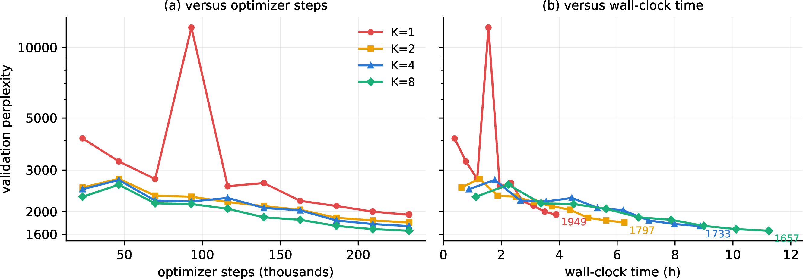
Figure 4: Split-FG tangent-count sweep on WikiText-103 with the reduced trunk step (\(\rho=0.03\); small8, one epoch per run, cosine schedule): validation perplexity versus optimizer steps (left)
and versus wall-clock time (right) for \(K\in\{1,2,4,8\}\). Perplexity improves monotonically in \(K\) (\(546.8\to361.5\)) at constant peak memory (\(811\) MiB; Table ¿tbl:tab:k-ablation?), and every \(K\) converges below the frozen-trunk control (dotted, \(667.6\))—even \(K{=}1\). On the wall-clock axis the curves share a common frontier, so \(K\) trades time for variance; comparisons across \(K\) are schedule-confounded, since
each run anneals over its own full epoch..
| \(K\) | JVPs/step | Final PPL | Val.NLL | Step time | Peak mem. |
|---|---|---|---|---|---|
| \(1\) | \(1\) | \(546.8\) | \(6.304\) | \(52\) ms | \(811\) MiB |
| \(2\) | \(2\) | \(437.6\) | \(6.081\) | \(62\) ms | \(811\) MiB |
| \(4\) | \(4\) | \(386.7\) | \(5.958\) | \(134\) ms | \(811\) MiB |
| \(8\) | \(8\) | \(361.5\) | \(5.890\) | \(187\) ms | \(811\) MiB |
12.6.0.1 Memory measurement.
We report peak GPU memory from torch.cuda.max_memory_allocated, reset at the start of each run. The same statistic is used for matched backpropagation and Split-FG so that \(\mathrm{MemSave}\) in
Eq. equation 21 measures the effect of removing trunk backpropagation. The run is carried out on a single NVIDIA RTX 4070 laptop GPU with 8GB VRAM. Full validation runs under torch.no_grad(), but it is still
part of the measured process and is therefore included in the peak-memory trace if it exceeds the training peak.
12.7 GPT Model Architecture↩︎
The GPT model is a causal transformer trained from random initialization. The default Split-FG decomposition places the split immediately before the linear LM head: the trunk computation maps token ids to hidden states through the token lookup, positional embeddings, all transformer blocks, and final LayerNorm, and the head is a large vocabulary projection \(hW_{\mathrm{out}}^\top+b\). In the reported runs, the vocabulary table used by the output projection is assigned to the exact head group, together with the LM-head bias; its token-lookup role is held fixed with respect to the trunk JVP. The forward-mode trunk JVP covers the positional table, transformer blocks, and final LayerNorm. Table ¿tbl:tab:gpt-arch? lists the concrete 8GB architecture.
| Layer | Operation | Output shape | Description |
|---|---|---|---|
| Input | Token ids | \((B,T)\) | Next-token language modelling windows, \(B=4\), \(T=128\). |
| Embedding | Token \(+\) position | \((B,T,256)\) | Token lookup plus learned positional table; the vocabulary table’s lookup role is held outside the trunk JVP. |
| Blocks \(1\ldots4\) | Causal self-attention \(+\) MLP | \((B,T,256)\) | Four transformer blocks, \(4\) heads, feed-forward width \(1024\), GELU activations. |
| Final norm | LayerNorm | \((B,T,256)\) | Final normalization before the LM head. |
| — trunk / head split — | |||
| LM head | Linear vocabulary projection | \((B,T,50257)\) | Logits \(=hW_{\mathrm{out}}^\top+b\); the vocabulary table and \(b\) receive the exact CE head gradient. |
| Output | CE loss | scalar | Cross-entropy over all token positions. |