Updating zigzag representatives efficiently
July 17, 2026
Abstract
Computation of zigzag persistence has progressed in recent years, with results showing that complexities of many problems closely align with those in the non-zigzag setting. The major efficiency gap now lies in the updating of zigzag representatives. In this paper, we propose efficient algorithms for updating zigzag representatives based on a recent algorithm for extracting zigzag representatives from a \(R=DV\) decomposition of a constructed non-zigzag. The main difficulty for designing our update algorithms lies in the adjacency change occurring in two operations that elongate or shorten a filtration. Despite the adjacency change, we find that the update can still be done efficiently in quadratic time.
1 Introduction↩︎
In persistent homology, a barcode of a filtered topological space provides a quantitative summary of its homological features. While the bars in the barcode effectively identify the duration of significant homological features, the underlying geometry is not captured by these durations alone. Cycle representatives add the missing information by locating the specific features in the topological spaces as they are born and die. Designing algorithms to find representatives for the ordinary (non-zigzag) persistence has been fruitful because an ordinary representative consists of a single cycle at birth that is included into all subsequent spaces [1], [2]. As a result, a representative takes \(O(m)\) space to store and summing two representatives takes \(O(m)\) time, where \(m\) is the number of insertions in the filtration. Since most algorithms for computing ordinary representatives require adding representatives, the compact representation makes it possible to design efficient algorithms for computing the ordinary representatives.
In zigzag persistence, since simplices can enter and leave a filtration, a representative cycle at one step may not exist at a later time. Hence, representatives compatible with the zigzag, that is, ones diagonalizing the linear maps, take \(O(mn)\) space each, where \(m\) is the number of insertions and deletions in the filtration and \(n\) is the maximum size of any complex. As as result, summing two such representatives takes \(O(mn)\) time. Perhaps this is why the time complexity for updating zigzag representatives still cannot catch up with the ordinary case, considering that almost all other computational results for zigzags match the complexity for the ordinary case [3], [4]. Specifically, the work [3] proposes algorithms for updating zigzag barcodes over eight elementary operations allowing a filtration to be transformed into any other one. Time complexities for all the operations in [3] match the ordinary case, e.g., they show that elongating or shortening a zigzag filtration can be done in \(O(m^2)\) time. However, their approach does not directly generalize to an efficient update of zigzag representatives, because the representatives maintained for the constructed up-down filtrations do not directly translate to representatives for the original zigzag.
In this paper, we provide efficient update algorithms for zigzag representatives whose complexity matches the ordinary case, with the only extra cost to output the representatives, a cost that cannot be avoided. Our update algorithms are built on a recent work [4] on extracting zigzag representatives efficiently from the \(R=DV\) decomposition [1] of a constructed non-zigzag filtration. In a nutshell, the authors [4] show that a zigzag representative in homological dimension \(p\) can be extracted from a column of the matrix \(R\) or \(V\) in \(O(p\cdot m\log m+C)\) time, where \(C\) is the size of the representative. This is almost as efficient as it can get because in most settings \(C\) dominates the \(p\cdot m\log m\) term. Relying on these results, we provide efficient update algorithms for the \(R=DV\) decomposition constructed for the ordinary filtration derived from the zigzag. This allows us to extract the representatives using methods in [4]. Time complexities for updating \(R=DV\) decomposition over the eight operations match those in the non-zigzag case: operations that transpose two inclusions run in \(O(m)\) time and operations that elongate or shorten a filtration run in \(O(m^2)\) time.
Since the update of zigzag representatives eventually boils down to updating the ordinary representatives in \(R=DV\), why not just use the existing update algorithms [1], [5]? We find that, among the eight operations, six of them can be easily updated using existing algorithms [1]. However, the remaining two operations, specifically, the outward expansions and contractions (see 2.1), cannot be implemented using existing approaches because of an adjacency change on the simplices (see 4.1). In particular, the transposition algorithm [1] and the removal algorithm [5] assume that boundaries of simplices stay the same before and after the update, which is not the case in the outward expansions and contractions. Hence, we mainly focus on addressing the update of \(R=DV\) for the two operations causing adjacency changes; see [sec:out-contra,sec:out-exp].
2 Background↩︎
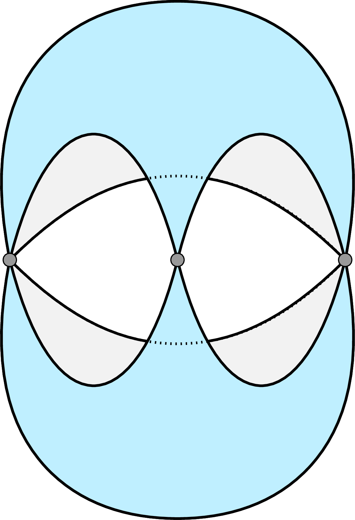
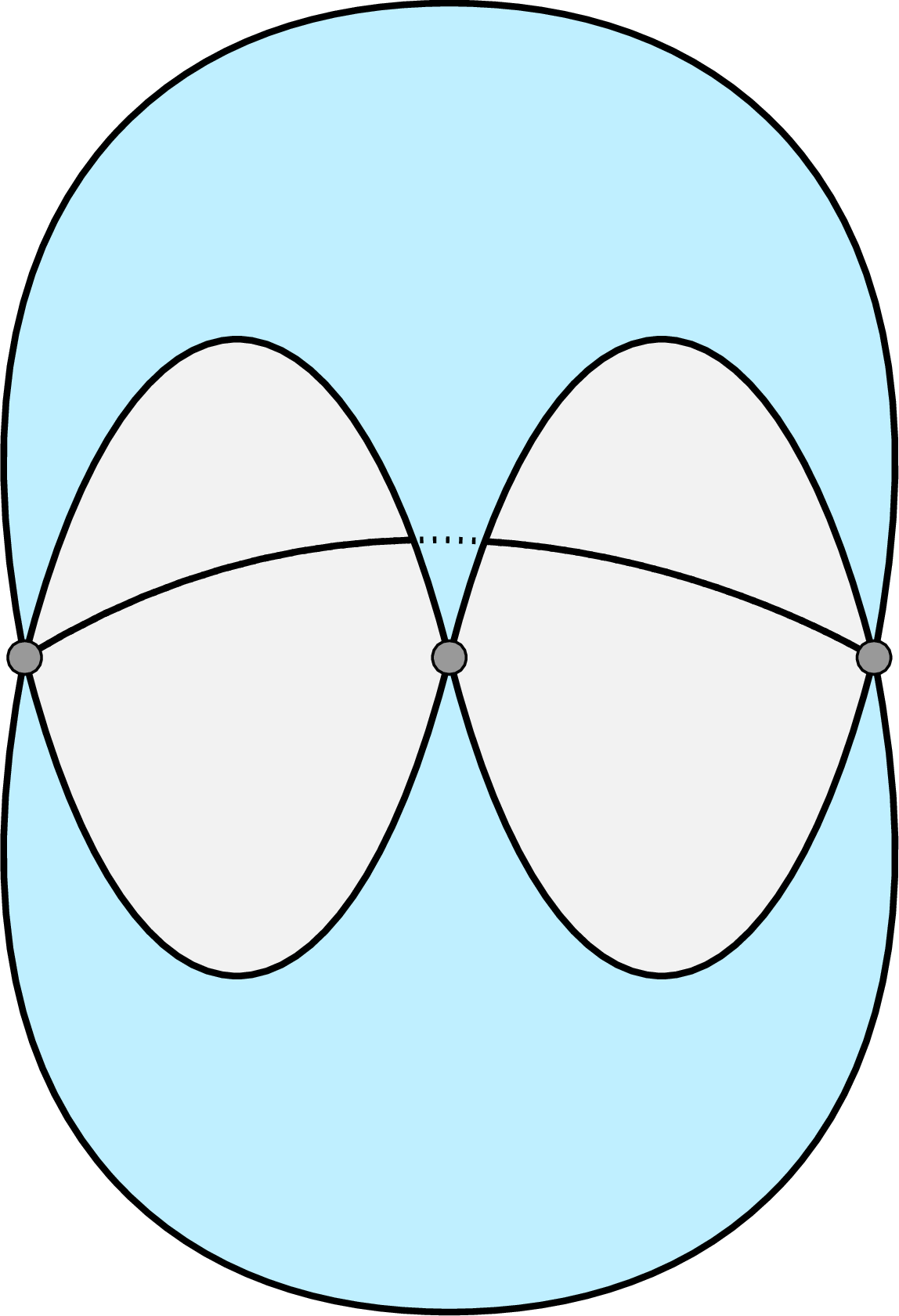
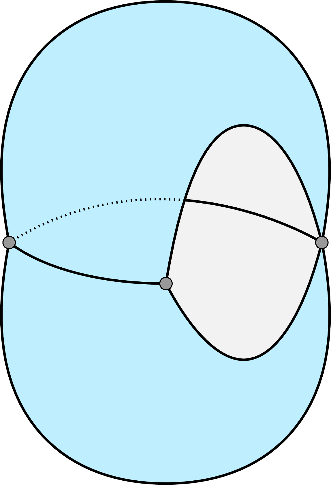
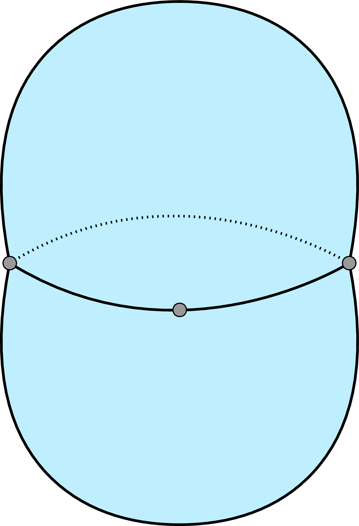
Figure 1: Examples [6] of \(\Delta\)-complexes with two triangles having the same set of vertices sharing 0, 1, 2, or 3 edges on their boundaries..
While the inputs all consist of simplicial complexes, algorithms in this paper internally work on \(\Delta\)-complexes [7], [8] by using of the conversion in [4], [6]. Building blocks of \(\Delta\)-complexes are called cells or \(\Delta\)-cells, which are similar to simplices but could share common faces in more relaxed ways; see 1 for examples and also [7], [8] for a formal definition. A zigzag filtration (or simply filtration) is a sequence of \(\Delta\)-complexes \[\mathcal{F}: K_0 \leftrightarrow K_1 \leftrightarrow \cdots \leftrightarrow K_m,\] in which each \(K_i\leftrightarrow K_{i+1}\) is either a forward inclusion \(K_i\hookrightarrow K_{i+1}\) (an insertion of cells) or a backward inclusion \(K_i\hookleftarrow K_{i+1}\) (a deletion of cells). Applying the homology functor \(H\) over all degrees with coefficients in a field \(\Bbbk\), we obtain a zigzag module \[H(\mathcal{F}): H(K_0) \leftrightarrow H(K_1) \leftrightarrow \cdots \leftrightarrow H(K_m),\] where each \(H(K_i)\leftrightarrow H(K_{i+1})\) is a linear map induced by inclusion. In this paper, we present our ideas with \(\Bbbk=\mathbb{Z}_2\) for simplicity; some details regarding generalizing to arbitrary fields are discussed in 9. The zigzag module \(H(\mathcal{F})\) has a decomposition [9], [10] of the form \[\label{eqn:inv-decomp} H(\mathcal{F})=\bigoplus_{k=1}^\ell\mathbb{I}^{[b_k,d_k]},\tag{1}\] in which each \(\mathbb{I}^{[b_k,d_k]}\) is an interval submodule of \(H(\mathcal{F})\). The (multi-)set of intervals \(\mathsf{Pers}(\mathcal{F}):=\{[b_k,d_k]\,|\,k=1,\ldots,\ell\}\) is an invariant of \(H(\mathcal{F})\) and is called the zigzag barcode of \(\mathcal{F}\).
Let \(Z(K_i)\) denote the cycle space (over all degrees) of \(K_i\). For a \([b_k,d_k]\in\mathsf{Pers}(\mathcal{F})\), a sequence of cycles \[z^k_{b_k}\in Z(K_{b_k}),z^k_{b_k+1}\in Z(K_{b_k+1}),\ldots,z^k_{d_k}\in Z(K_{d_k})\] is called its zigzag representative if each \([z^k_i]\) generates \(\mathbb{I}^{[b_k,d_k]}(i)\) for the interval summand \(\mathbb{I}^{[b_k,d_k]}\) in 1 . It follows: (1) \([z^k_i]\mapsto[z^k_{i+1}]\) or \([z^k_i]\mapsfrom[z^k_{i+1}]\) based on the direction of the map; (2) for each \(K_i\), \(\{[z^k_i]\mid i\in[b_k,d_k]\}\) is a basis for \(H(K_i)\).
In other words, all zigzag representatives for bars in \(\mathsf{Pers}(K_i)\) form compatible bases for spaces in \(H(\mathcal{F})\) such that linear maps in \(H(\mathcal{F})\) are diagonalized.
An inclusion in a filtration is called cell-wise if it is an addition or deletion of a single cell \(\sigma\), which we sometimes denote as, e.g., \(K_i\xleftrightarrow{\;\sigma\;}K_{i+1}\). A filtration is called cell-wise if it contains only cell-wise inclusions. For computation, zigzag filtrations in this paper are by default cell-wise; we also assume they start and end with empty complexes (as adopted in [4], [11], [12]). We note that any filtration can be converted into this form by expanding the inclusions and attaching complexes to both ends. Zigzag representatives for general filtrations can also be easily retrieved from those computed on simplex-wise ones; see [4] for details.
For a matrix \(A\), let \({A}[i,j]\) denote its element on the \(i\)-th row and \(j\)-th column. \({A}[i,\cdot]\) denotes its \(i\)-th row; \({A}[\cdot,j]\), its \(j\)-th column. The pivot of \({A}[\cdot,j]\) is the row index of the lowest non-zero entry of \({A}[\cdot,j]\) and is denoted \(\mathrm{piv}({A}[\cdot,j])\). Since columns and rows of matrices in this paper correspond to \(\Delta\)-cells, \(i\) and \(j\) could also be cells and \(\mathrm{piv}({A}[\cdot,j])\) could also refer to the cell corresponding to the row.
2.1 Update operations↩︎
We now present all the eight update operations considered in the paper. Note that these operations are sufficient to transform any simplex-wise zigzag filtration into another [3]. In this subsection, \(\mathcal{F}\) and \(\mathcal{F}^*\) are both simplex-wise zigzag filtrations consisting of simplicial complexes which start and end with \(\varnothing\).
Forward switch [11] swaps two forward inclusions and requires \(\sigma\nsubseteq\tau\): \[\tag{2} \begin{figure}\includegraphics[width=0.8\textwidth]{_pdflatex/msnbtrcv.png}\tag{3}\end{figure}\]
Backward switch swaps two backward inclusions and requires \(\tau\nsubseteq\sigma\): \[\tag{4} \begin{figure}\includegraphics[width=0.8\textwidth]{_pdflatex/ptqedhxi.png}\tag{5}\end{figure}\]
Outward/inward switch [9] swaps two inclusions of opposite directions and requires \(\sigma\neq\tau\): \[\tag{6} \begin{figure}\includegraphics[width=0.8\textwidth]{_pdflatex/lvbfmzce.png}\tag{7}\end{figure}\]
The switch from \(\mathcal{F}\) to \(\mathcal{F}^*\) is an outward switch and the switch from \(\mathcal{F}^*\) to \(\mathcal{F}\) is an inward switch. Notice that if \(\sigma=\tau\), then e.g., for outward switch, we cannot delete \(\tau\) from \(K_{i-1}\) in \(\mathcal{F}^*\) because \(\tau\not\in K_{i-1}\).
Inward contraction/expansion [11] is as follows: \[\tag{8} \begin{figure}\includegraphics[width=0.8\textwidth]{_pdflatex/lcrzxibe.png}\tag{9}\end{figure}\] From \(\mathcal{F}\) to \(\mathcal{F}^*\) we have an inward contraction and from \(\mathcal{F}^*\) to \(\mathcal{F}\) we have an inward expansion. We have \(K^*_{i}=K_{i-1}=K_{i+1}\). Because neither one of these complexes contains \(\sigma\), they also do not contain any of its cofaces.
Outward contraction/expansion is superficially similar to the inward version, but instead of removing successive addition and removal of a simplex, it fuses two different index-intervals over which the simplex appears in the filtration. The two center arrows now point away from each other: \[\tag{10} \begin{figure}\includegraphics[width=0.8\textwidth]{_pdflatex/fpgzhxml.png}\tag{11}\end{figure}\]
Notice that we also have \(K^*_{i}=K_{i-1}=K_{i+1}\).
2.2 Conversion to non-zigzag filtration↩︎
We review results from prior works that lay the groundwork for this paper. Specifically, we first describe how a zigzag filtration \(\mathcal{F}\) can be converted to a non-zigzag filtration \({\mathcal{F}_\mathrm{nz}}\) [6]. We then present a recent finding [4] on how representatives for \({\mathcal{F}_\mathrm{nz}}\) can be used to recover representatives for the original \(\mathcal{F}\) from an \(R=DV\) decomposition [1] for \({\mathcal{F}_\mathrm{nz}}\). In 3, we describe how to update the representatives after six of the eight operations described in 2.1; the update rules follow directly from the conversion.
Given a simplex-wise zigzag filtration \[\mathcal{F}: \varnothing= K_0\xleftrightarrow{\;\sigma_{0}\;} K_1\xleftrightarrow{\;\sigma_{1}\;} \cdots \xleftrightarrow{\;\sigma_{m-1}\;} K_m =\varnothing,\] where a simplex can be inserted and deleted multiple times, we first treat each occurrence of a simplex in \(\mathcal{F}\) as a distinct \(\Delta\)-cell, and have the following cell-wise zigzag filtration \[\label{eqn:fzz-up-sec-filt} \overline{\mathcal{F}}: \varnothing= \overline{K}_0\xleftrightarrow{\;\overline{\sigma}_{0}\;} \overline{K}_1\xleftrightarrow{\;\overline{\sigma}_{1}\;} \cdots \xleftrightarrow{\;\overline{\sigma}_{m-1}\;} \overline{K}_m =\varnothing.\tag{12}\] While \(\overline{\mathcal{F}}\) “looks” exactly the same as \(\mathcal{F}\), treating the simplices as \(\Delta\)-cells enables us to perform the subsequent conversion to a non-zigzag filtration \[{\mathcal{F}_\mathrm{nz}}: \{\omega\}=L_0\xhookrightarrow{\;\tau_0\;} \cdots\xhookrightarrow{\;\tau_{\ifthenelse{\equal{}{}}{n}{n_{}}-1}\;} L_{\ifthenelse{\equal{}{}}{n}{n_{}}} \xhookrightarrow{\;\hat{\tau}_{\ifthenelse{\equal{}{}}{n}{n_{}}}\;} {L}_{\ifthenelse{\equal{}{}}{n}{n_{}}+1} \cdots\xhookrightarrow{\;\hat{\tau}_{m-1}\;} {L}_{m}.\] Above, \(\omega\) is an additional vertex for coning; \(\tau_0,\tau_1,\ldots,\tau_{\ifthenelse{\equal{}{}}{n}{n_{}}-1}\) are \(\Delta\)-cells inserted in \(\overline{\mathcal{F}}\) with the same insertion order as in \(\overline{\mathcal{F}}\); \(\tau_{\ifthenelse{\equal{}{}}{n}{n_{}}},\tau_{\ifthenelse{\equal{}{}}{n}{n_{}}+1},\ldots,\tau_{m-1}\) are cones of \(\Delta\)-cells deleted in \(\overline{\mathcal{F}}\) with the deletion order in \(\overline{\mathcal{F}}\) reversed to form the insertion order in \({\mathcal{F}_\mathrm{nz}}\). See 2 for an example of the conversion. Notice that adjacency of cells in \(\overline{\mathcal{F}}\) is carried over to \({\mathcal{F}_\mathrm{nz}}\).

Figure 2: An example of converting a zigzag filtration of simplices to a non-zigzag filtration of \(\Delta\)-cells, where \(\mathcal{F}\) and \(\overline{\mathcal{F}}\) look the same and only \(\overline{\mathcal{F}}\) is listed. Note that \(\mathcal{F},{\mathcal{F}_\mathrm{nz}}\) both start with the complexes \(\varnothing\) and \(\{v_0\}\) which are omitted for brevity. The simplex \(\{v_0,v_1\}\) is inserted twice in \(\mathcal{F}\) with the two insertions corresponding two different \(\Delta\)-cells \(e_0\), \(e_1\) in \(\overline{\mathcal{F}}\). Insertions of \(e_0\), \(e_1\) in \(\overline{\mathcal{F}}\) correspond to the same insertions of them in the first half of \({\mathcal{F}_\mathrm{nz}}\), while deletions of \(e_0\), \(e_1\), \(v_1\), \(v_0\) in \(\overline{\mathcal{F}}\) corresponds to insertions of the cones \(\omega\cdot v_0\), \(\omega\cdot v_1\), \(\omega\cdot e_1\), \(\omega\cdot e_0\) in the second half of \({\mathcal{F}_\mathrm{nz}}\), with the order reversed..
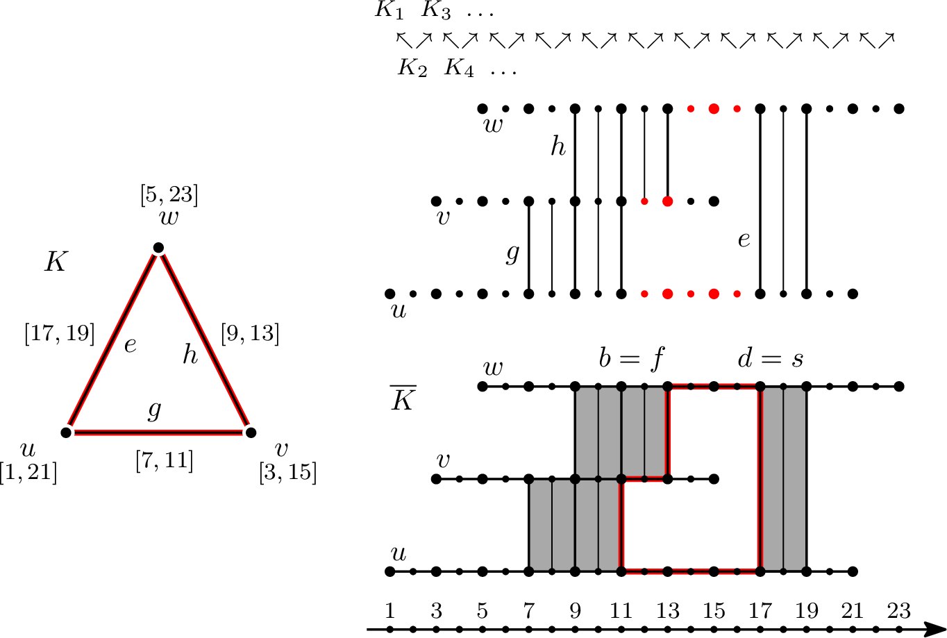
Figure 3: An example for retrieving zigzag representatives from the converted non-zigzag filtration. The input zigzag filtration is on top. The total (last) complex \(K\) of the converted non-zigzag filtration is on left, with labels being lifetimes of simplices in the zigzag filtration. The constructed prism \(\overline{K}\) and its levelset zigzag are at bottom. The red cycle in \(K\) is used to construct a representative for the zigzag bar \([12,16]\). The red cycle in \(\overline{K}\) is the apex representative constructed. Slices of the apex representative provide the zigzag representative (vertices colored in red) for \([12,16]\). Figure from [4]..
Let \(D\) be the filtered boundary matrix for \({\mathcal{F}_\mathrm{nz}}\), i.e., \(D\) encodes the boundary operator \(\partial\) with the cells ordered according to \({\mathcal{F}_\mathrm{nz}}\). Let \(R\), \(V\) be square matrices with the same dimension as \(D\). We call a decomposition of the form \[\label{eqn:decomp-all} R=DV\tag{13}\] valid if \(V\) is upper-triangular and has all 1’s on the diagonal. The decomposition is further called reduced if non-zero columns of \(R\) have distinct pivots. One can read off the barcode \(\mathsf{Pers}({\mathcal{F}_\mathrm{nz}})\) and the representatives from a reduced decomposition [13]. Moreover, there is a bijection between \(\mathsf{Pers}(\mathcal{F})\) and \(\mathsf{Pers}({\mathcal{F}_\mathrm{nz}})\) so that \(\mathsf{Pers}(\mathcal{F})\) could be recovered from \(\mathsf{Pers}({\mathcal{F}_\mathrm{nz}})\) with an overall complexity of \(O(m)\) for the conversion [6]. Recently, the authors of [4] showed that one could also recover the representatives for the bars in \(\mathsf{Pers}(\mathcal{F})\) from a reduced decomposition as in 13 . They construct a prism complex \(\overline{K}\) with a real-valued function \(\overline{f}\), whose levelset zigzag [14], \(\mathsf{LPers}(\overline{f})\), is isomorphic to the zigzag persistence of \(\mathcal{F}\), \(\mathsf{Pers}(\mathcal{F})=\mathsf{LPers}(\overline{f})\). They turn to the Mayer-Vetoris pyramid [14] of function \(\overline{f}\) and define apex representatives, from which the representatives of \(\mathsf{Pers}(\mathcal{F})\) can be efficiently retrieved (see 3 for an example). Their main result is summarized in the following theorem.
Theorem 1 ([4]). Given a reduced decomposition \(R = DV\) for \({\mathcal{F}_\mathrm{nz}}\), for each \(q\)-dimensional bar \([b,d]\in\mathsf{Pers}(\mathcal{F})\) and its corresponding persistence pair \((\sigma,\tau)\) in \(\mathsf{Pers}({\mathcal{F}_\mathrm{nz}})\), one can retrieve the apex representative \(\Gamma\) for the corresponding bar in \(\mathsf{LPers}(\overline{f})\) from \(R[\tau]\) or \(V[\tau]\) in \(O(q\cdot m\log m)\) time. Moreover, the zigzag representative for \([b,d]\in\mathsf{Pers}(\mathcal{F})\) can be retrieved from \(\Gamma\) in \(O(\log m+C)\) time, where \(C\) is the size of the output.
3 Easy updates↩︎
In this section we present the update for six of the operations in 2.1. The update algorithms for outward contraction and expansion involving the adjacency change are presented in [sec:out-contra,sec:out-exp] respectively. For all the updates, we assume that we are given a reduced decomposition as in 13 for the non-zigzag filtration that corresponds to the zigzag filtration before the operation, and the goal is to obtain a reduced decomposition for the non-zigzag filtration after the operation. Representatives for the zigzag filtrations can then be extracted using 1.
Since the switch in 6 swaps two inclusions of different directions, the corresponding non-zigzag filtrations before and after the switch are the same. So no update to the \(R=DV\) decomposition is necessary.
Corresponding to a forward switch in 2 on the original zigzag filtration, there is a forward switch in the first half of the non-zigzag filtration consisting of the base cells. Similarly, corresponding to a backward switch in 4 on the zigzag filtration, there is a forward switch in the second half of the non-zigzag filtration consisting of the cone cells. To perform the update for a forward switch on a non-zigzag filtration, we utilize the \(O(m)\) transposition algorithm in [1].
Let \({\mathcal{F}_\mathrm{nz}}\) (resp.\(\mathcal{F}^*_\mathrm{nz}\)) be the non-zigzag filtration corresponding to \(\mathcal{F}\) (resp.\(\mathcal{F}^*\)) in 8 . Also, let \(\sigma_0\) be the \(\Delta\)-cell in \({\mathcal{F}_\mathrm{nz}}\) corresponding to the insertion \(K_{i-1}\xhookrightarrow{\;\sigma\;}K_{i}\) in \(\mathcal{F}\) and let \(\hat{\sigma}_0\) be the cone of \(\sigma_0\) corresponding to the deletion \(K_{i}\xhookleftarrow{\;\sigma\;}K_{i+1}\) in \(\mathcal{F}\). Since \(\sigma\) is deleted immediately after it is inserted to \(K_{i}\) in \(\mathcal{F}\), we have that \(\sigma_0\) has no cofaces in \({\mathcal{F}_\mathrm{nz}}\). This also implies that \(\hat{\sigma}_0\) has no cofaces in \({\mathcal{F}_\mathrm{nz}}\). To perform the update for an inward expansion, suppose that we are given a reduced decomposition \(R^{*}=D^{*}V^{*}\) for \(\mathcal{F}^*_\mathrm{nz}\) before the expansion. We first append columns representing the chains \(\sigma_0\), \(\hat{\sigma}_0\) to \(V^{*}\), and columns representing \(\partial\sigma_0\), \(\partial\hat{\sigma}_0\) to \(R^{*}\). Notice that we also need to append new rows corresponding to \(\sigma_0\), \(\hat{\sigma}_0\) to \(R^{*}\) and \(V^{*}\). Call the newly derived matrices \(R\) and \(V\). We then perform two column reductions [15] to make \(R\) reduced, which takes \(O(m^2)\) time. After this, we perform \(O(m)\) row/column transpositions on \(R\) and \(V\) using the algorithm in [1] to place the columns and rows of \(\sigma_0\), \(\hat{\sigma}_0\) to the appropriate positions as in \({\mathcal{F}_\mathrm{nz}}\). Thus, the update for inward expansion takes \(O(m^2)\) time.
We now describe the update for an inward contraction. Suppose that we are given a reduced decomposition \(R=DV\) for \({\mathcal{F}_\mathrm{nz}}\). We first perform \(O(m)\) transpositions [1] so that the columns (resp.rows) corresponding to \(\sigma_0\) and \(\hat{\sigma}_0\) are the last two columns (resp.rows) in \(R\) and \(V\). Notice that we could do this because \(\sigma_0\), \(\hat{\sigma}_0\) have no cofaces in \({\mathcal{F}_\mathrm{nz}}\). We then simply remove the columns and rows of \(\sigma_0\) and \(\hat{\sigma}_0\) from \(R\) and \(V\). Accordingly, the update for the inward contraction also takes \(O(m^2)\) time.
The fact that \(\sigma_0\) and \(\hat{\sigma}_0\) have no cofaces in the converted non-zigzag filtration is a key condition that allows existing algorithms to be applied. The outward contraction and expansion, however, do not have such a property, which makes them more difficult. In fact, there is certain non-trivial change on the cell adjacency over the two operations, which is detailed in 4.1.
4 Outward contraction↩︎
We present the update algorithm for an outward contraction. Recall that an outward contraction is the following operation: \[\tag{14} \begin{figure}\includegraphics[width=0.8\textwidth]{_pdflatex/fkxwsvqd.png}\tag{15}\end{figure}\] where \(K^*_{i}=K_{i-1}=K_{i+1}\) and \(\sigma\) is a \(p\)-simplex.
Let \({\mathcal{F}_\mathrm{nz}}\) and \(\mathcal{F}^*_\mathrm{nz}\), respectively, be the non-zigzag filtrations corresponding to \(\mathcal{F}\) and \(\mathcal{F}^*\) by the conversion in 2.2. Rather than consider a decomposition over all degrees as in 13 , we work on a separate decomposition for each degree. Specifically, for each \(q\), let \(D_q\) (resp.\(D^*_q\)) be the \(q\)-th filtered boundary matrix for \({\mathcal{F}_\mathrm{nz}}\) (resp.\(\mathcal{F}^*_\mathrm{nz}\)) which encodes the boundary operator \(\partial_q:C_q\to C_{q-1}\). We assume that we are given a reduced decomposition \[R_q=D_qV_q\] for each \(q\), where \(R_q\) has the same dimension as \(D_q\) (i.e., rows corresponding to \((q-1)\)-cells and columns corresponding to \(q\)-cells), and \(V_q\) is a square matrix with both rows and columns corresponding to \(q\)-cells. The goal of the update is to compute the decompositions for \(\mathcal{F}^*_\mathrm{nz}\).
4.1 Changes on the boundary matrices↩︎
To present our update strategy, we first describe the changes from the boundary matrix \(D_{q}\) to \(D^*_{q}\) for the different \(q\). In a zigzag filtration, each insertion of a simplex \(\kappa\) is associated with a deletion of \(\kappa\), which determines the time interval of a specific occurrence of \(\kappa\). Also notice that a coface of \(\kappa\) must have its time intervals contained in those of \(\kappa\). In 16 , we illustrate the corresponding insertion and deletion for the two arrows \(K_{i-1}\xhookleftarrow{\;\sigma\;}K_i\xhookrightarrow{\;\sigma\;}K_{i+1}\): \[\tag{16} \opt{arXiv}{\scalebox{1.1}}{\begin{figure}\includegraphics[width=0.8\textwidth]{_pdflatex/jrmkawqc.png}\tag{17}\end{figure}}\] We suppose there are \((p+1)\)-cofaces \(\tau\), \(\tau'\) of \(\sigma\) whose time intervals are contained in the two intervals of \(\sigma\) respectively. In 16 , we also illustrate the filtration \(\overline{\mathcal{F}}\) consisting of the \(\Delta\)-complexes as in 2.2, where \(\sigma_1\), \(\sigma_2\) are \(\Delta\)-cells corresponding to the two occurrences of \(\sigma\) in \(\mathcal{F}\) respectively, and \(\tau_0\), \(\tau'_0\) are \(\Delta\)-cells corresponding to \(\tau\), \(\tau'\) respectively. By the conversion in 2.2, \(\sigma_1\) is a \(p\)-face of \(\tau_0\) and \(\sigma_2\) is a \(p\)-face of \(\tau'_0\) in \(\overline{\mathcal{F}}\). Notice that the adjacency is also carried over to the non-zigzag filtration \({\mathcal{F}_\mathrm{nz}}\).
18 illustrates the adjacency of the simplices/cells in \(\mathcal{F}^*\) and \(\overline{\mathcal{F}^*\mkern-6mu}\mkern 6mu\) after the contraction: \[\tag{18} \opt{arXiv}{\scalebox{1.1}}{\begin{figure}\includegraphics[width=0.8\textwidth]{_pdflatex/wjlhakpg.png}\tag{19}\end{figure}}\] The insertion of \(\sigma\) before \(K_{i-1}\xhookleftarrow{\;\sigma\;}K_i\xhookrightarrow{\;\sigma\;}K_{i+1}\) in \(\mathcal{F}\) and the deletion of \(\sigma\) after, now become the endpoints of the same time interval in \(\mathcal{F}^*\). As a result, the \(\Delta\)-cell \(\sigma_0\) corresponding to \(\sigma\) now becomes a \(p\)-face of \(\tau_0\), \(\tau'_0\) in \(\overline{\mathcal{F}^*\mkern-6mu}\mkern 6mu\) as well as in \(\mathcal{F}^*_\mathrm{nz}\). The above change applies to any \((p+1)\)-cofaces of \(\sigma_1\), \(\sigma_2\) in \(\overline{\mathcal{F}}\) and \({\mathcal{F}_\mathrm{nz}}\). In other words, the two \(p\)-cells \(\sigma_1\), \(\sigma_2\) in \({\mathcal{F}_\mathrm{nz}}\) are identified as the same \(p\)-cell \(\sigma_0\) in \(\mathcal{F}^*_\mathrm{nz}\). Since cell insertions in the first half of \(\mathcal{F}^*_\mathrm{nz}\) follow the same order as cell insertions in \(\overline{\mathcal{F}^*\mkern-6mu}\mkern 6mu\), \(\sigma_0\) in \(\mathcal{F}^*_\mathrm{nz}\) corresponds to \(\sigma_1\) in \({\mathcal{F}_\mathrm{nz}}\). The change in the second halves of \({\mathcal{F}_\mathrm{nz}}\) and \(\mathcal{F}^*_\mathrm{nz}\) which involve the cone cells is similar. However, since the insertion order of cone cells in \({\mathcal{F}_\mathrm{nz}}\) (resp.\(\mathcal{F}^*_\mathrm{nz}\)) is the reverse of the deletion order of cells in \(\overline{\mathcal{F}}\) (resp.\(\overline{\mathcal{F}^*\mkern-6mu}\mkern 6mu\)), the cone \(\hat{\sigma}_0\) of \({\sigma}_0\) in \(\mathcal{F}^*_\mathrm{nz}\) now corresponds to the cone \(\hat{\sigma}_2\) of \({\sigma}_2\) in \({\mathcal{F}_\mathrm{nz}}\).
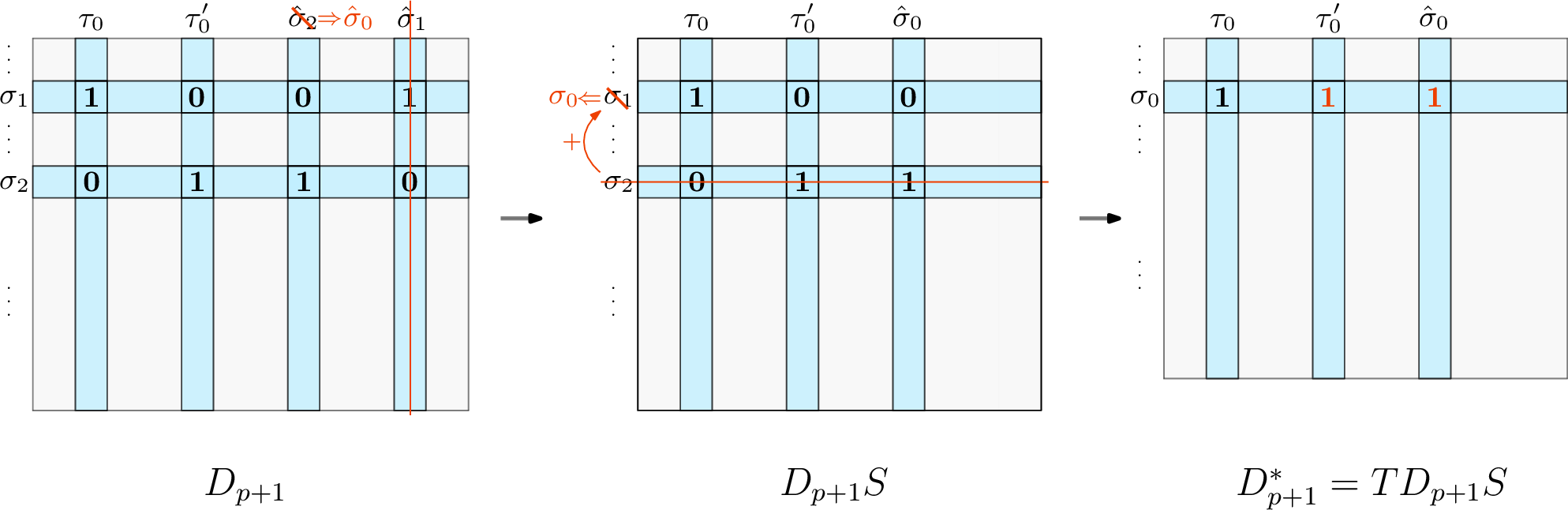
Figure 4: Change from boundary matrix \(D_{p+1}\) to \(D^*_{p+1}\) (see 20 for definitions of \(S\) and \(T\))..
We summarize the change as follows:
From \({\mathcal{F}_\mathrm{nz}}\) to \(\mathcal{F}^*_\mathrm{nz}\), the \(p\)-cell \(\sigma_2\) and the \((p+1)\)-cell \(\hat{\sigma}_1\) are removed, the \(p\)-cell \(\sigma_1\) and the \((p+1)\)-cell \(\hat{\sigma}_2\) are renamed as \(\sigma_0\) and \(\hat{\sigma}_0\) respectively, and \((p+1)\)-cofaces of \(\sigma_1\), \(\sigma_2\) (resp.\((p+2)\)-cofaces of \(\hat{\sigma}_1\), \(\hat{\sigma}_2\)) now have \(\sigma_0\) (resp.\(\hat{\sigma}_0\)) as face. Accordingly, the change from the boundary matrix \(D_{q}\) to \(D^*_{q}\) for the different \(q\) can be described as follows:
\(D_{p+1}\) to \(D^*_{p+1}\): the column of \(\hat{\sigma}_1\) is removed, and column label \(\hat{\sigma}_2\) is changed to \(\hat{\sigma}_0\); the row of \(\sigma_2\) is added to the row of \(\sigma_1\), with the row of \(\sigma_2\) removed, and the row label \(\sigma_1\) changed to \(\sigma_0\); see 4.
\(D_{p}\) to \(D^*_{p}\): the column of \(\sigma_2\) is removed, and the column label \(\sigma_1\) is changed to \(\sigma_0\).
\(D_{p+2}\) to \(D^*_{p+2}\): the row of \(\hat{\sigma}_1\) is added to the row of \(\hat{\sigma}_2\), with the row of \(\hat{\sigma}_1\) removed, and the row label \(\hat{\sigma}_2\) changed to \(\hat{\sigma}_0\).
We also have \(D_{q}=D^*_{q}\) for any other \(q\).
4.2 Update for degree \(p+1\)↩︎
We describe in detail the update for degree \(p+1\), i.e., given the decomposition \[R_{p+1}=D_{p+1}V_{p+1}\] for \({\mathcal{F}_\mathrm{nz}}\), we find the corresponding decomposition for \(\mathcal{F}^*_\mathrm{nz}\). The updates for the degrees \(p\), \(p+2\) are similar but simpler; they are briefly described in 4.3.
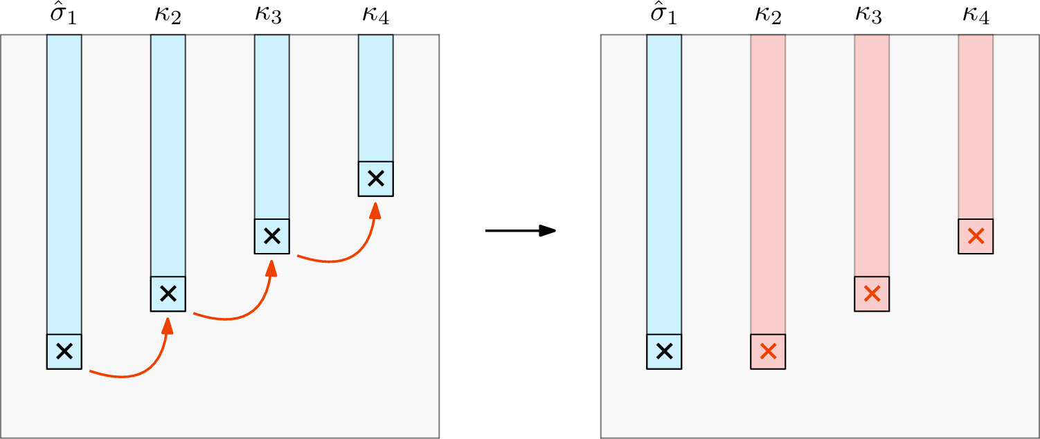
Figure 5: An illustration of columns in \(R_{p+1}\) whose corresponding columns in \(V_{p+1}\) have non-zero values on \(\hat{\sigma}_1\) in Step I.2, where \(\ell=4\). Pivots of these columns in \(R_{p+1}\) are monotonically decreasing before the column summation in Step I.2, with the red arrows indicating the direction of the summation. Note that we perform the summation starting from the right-most two columns so that after this, only pivot of the column of \(\hat{\sigma}_1\) may clash with another one. The clash is fixed later on..
We first perform column summations on \(V_{p+1}\), and correspondingly on \(R_{p+1}\), to make the row \({V_{p+1}}[\hat{\sigma}_1,\cdot]\) contain zero entries everywhere except on the diagonal. The aim is to remove the reference to \(\hat{\sigma}_1\) in \(V_{p+1}\) to prepare for the later removal of \(\hat{\sigma}_1\). To ensure a valid decomposition, we only perform left-to-right column summations so that \(V_{p+1}\) is still an upper triangular matrix with 1’s on the diagonal. We also ensure \(R_{p+1}\) has distinct column pivots almost everywhere, possibly with a single violation which will be fixed later.
There are two cases for the step. First, if \({R_{p+1}}[\cdot,\hat{\sigma}_1]=0\), i.e., \({V_{p+1}}[\cdot,\hat{\sigma}_1]\) is a cycle, then we only need to add \({V_{p+1}}[\cdot,\hat{\sigma}_1]\) to any other \({V_{p+1}}[\cdot,\kappa]\) with \({V_{p+1}}[\hat{\sigma}_1,\kappa]\neq 0\), without needing to change \({R_{p+1}}[\cdot,\kappa]\).
Now suppose that \({R_{p+1}}[\cdot,\hat{\sigma}_1]\neq 0\). We have two separate sub-steps (note that these two sub-steps bear some similarity to the SiRUP algorithm [5] that considers removing a simplex without cofaces from a non-zigzag filtration).
Step I.1: While there are two columns \({V_{p+1}}[\cdot,\kappa]\) and \({V_{p+1}}[\cdot,\nu]\), \(\kappa<\nu\), with non-zero entries on \(\hat{\sigma}_1\) such that \[\mathrm{piv}({R_{p+1}}[\cdot,\kappa])<\mathrm{piv}({R_{p+1}}[\cdot,\nu]),\] add \({V_{p+1}}[\cdot,\kappa]\) to \({V_{p+1}}[\cdot,\nu]\) and \({R_{p+1}}[\cdot,\kappa]\) to \({R_{p+1}}[\cdot,\nu]\), so that \({V_{p+1}}[\hat{\sigma}_1,\nu]=0\) and the pivot of \({R_{p+1}}[\cdot,\nu]\) stays the same.
Step I.2: Let \[{V_{p+1}}[\cdot,\kappa_1],\ldots,{V_{p+1}}[\cdot,\kappa_\ell]\] be all columns in \(V_{p+1}\) that still have non-zero entries on \(\hat{\sigma}_1\), where \[\kappa_1=\hat{\sigma}_1<\kappa_2<\cdots<\kappa_\ell.\] We have \[{\mathrm{piv}}({R_{p+1}}[\cdot,\kappa_1])>\cdots>\mathrm{piv}({R_{p+1}}[\cdot,\kappa_\ell])\] because if \(\mathrm{piv}({R_{p+1}}[\cdot,\kappa_j])<\mathrm{piv}({R_{p+1}}[\cdot,\kappa_{j+1}])\) for a \(j\), then \({V_{p+1}}[\hat{\sigma}_1,\kappa_{j+1}]\) would have been set to zero in Step I.1. Also notice that \(\kappa_1,\ldots,\kappa_\ell\) are at the Pareto front of the partial order defined by the order of column indices and the order of pivots in \(R_{p+1}\). See 5 for an example of \(\ell=4\).
We then do the following:
- For \(j=\ell,\ell-1,\ldots,2\), add \({R_{p+1}}[\cdot,\kappa_{j-1}]\) to \({R_{p+1}}[\cdot,\kappa_j]\) and \({V_{p+1}}[\cdot,\kappa_{j-1}]\) to \({V_{p+1}}[\cdot,\kappa_j]\).
After Step I.2, the row \({V_{p+1}}[\hat{\sigma}_1,\cdot]\) has zero entries everywhere except on the diagonal. Moreover, for each \(j\), the pivot of \({R_{p+1}}[\cdot,\kappa_j]\) after Step I.2 equals the pivot of \({R_{p+1}}[\cdot,\kappa_{j-1}]\) before Step I.2. Hence, columns of \(R_{p+1}\) have distinct pivots everywhere except \({R_{p+1}}[\cdot,\hat{\sigma}_{1}]\), for which \(\mathrm{piv}({R_{p+1}}[\cdot,\hat{\sigma}_{1}])=\mathrm{piv}({R_{p+1}}[\cdot,\kappa_{2}])\).
If \(\ell=1\) in Step I.2, then no column summations are needed, and columns of \(R_{p+1}\) have distinct pivots after Step I.2.
Notice that the change from \(D_{p+1}\) to \(D^*_{p+1}\) involves row and column operations that can be expressed as multiplication of \(D_{p+1}\) on the left and right by suitable matrices. Specifically, let \(\ifthenelse{\equal{q}{}}{n}{n_{q}}\), \(\ifthenelse{\equal{q}{}}{n^*}{n^*_{q}}\) be the number of \(q\)-cells in \({\mathcal{F}_\mathrm{nz}}\), \(\mathcal{F}^*_\mathrm{nz}\), respectively. We have \[\label{eqn:dmat-mult} D^*_{p+1}=TD_{p+1}S,\tag{20}\] where \(T\) is an \(\ifthenelse{\equal{p}{}}{n^*}{n^*_{p}}\times\ifthenelse{\equal{p}{}}{n}{n_{p}}\) matrix representing the following row operations:
\({D^*_{p+1}}[\sigma_0,\cdot]={D_{p+1}}[\sigma_1,\cdot]+{D_{p+1}}[\sigma_2,\cdot]\);
\({D^*_{p+1}}[\kappa,\cdot]={D_{p+1}}[\kappa,\cdot]\) for any \(\kappa\neq\sigma_0\) in \(\mathcal{F}^*_\mathrm{nz}\).
Similarly, \(S\) is an \(\ifthenelse{\equal{p+1}{}}{n}{n_{p+1}}\times\ifthenelse{\equal{p+1}{}}{n^*}{n^*_{p+1}}\) matrix which removes the column of \(\hat{\sigma}_1\) from \(D_{p+1}\). See 4.
Now let \[\label{eqn:rvmat-mult} R^*_{p+1}=TR_{p+1}S\text{ and }V^*_{p+1}=S^\mathsf{T}V_{p+1}S,\tag{21}\] where \(S^\mathsf{T}\) removes the row of \(\hat{\sigma}_1\) from \(V_{p+1}\). We have:
\(R^*_{p+1}=D^*_{p+1}V^*_{p+1}\).
Proof. By [eqn:dmat-mult,eqn:rvmat-mult], we need to show \[TR_{p+1}S=TD_{p+1}SS^\mathsf{T}V_{p+1}S,\] which is to show \[\label{eqn:RT-DTTVT} R_{p+1}S=D_{p+1}SS^\mathsf{T}V_{p+1}S.\tag{22}\] Let \(I^\circ=SS^\mathsf{T}\). We have that the only difference between \(I^\circ\) and an identity matrix is that the diagonal entry in \(I^\circ\) corresponding to \(\hat{\sigma}_1\) is zero; see 6. Multiplying by \(I^\circ\) on the left of \(V_{p+1}\) then sets the row of \(\hat{\sigma}_1\) to zero. However, since only the diagonal entry in the row \({V_{p+1}}[\hat{\sigma}_1,\cdot]\) is non-zero, \(V_{p+1}\) and \(I^\circ V_{p+1}\) differ only in the columns corresponding to \(\hat{\sigma}_1\). Since \(R_{p+1}=D_{p+1}V_{p+1}\), we also have that \(R_{p+1}\) and \(D_{p+1}I^\circ V_{p+1}\) differ only in the columns corresponding to \(\hat{\sigma}_1\). Since multiplying by \(S\) on the right removes the column corresponding to \(\hat{\sigma}_1\), we then have 22 . ◻
[prop:Rx-DxVx] provides the initial decomposition for \(\mathcal{F}^*_\mathrm{nz}\) that we work on. Notice that while \(V^*_{p+1}\) is still upper triangular with all 1’s on the diagonal, \(R^*_{p+1}\) may not necessarily have distinct column pivots. By [obsv:I-2-pivots] and the fact that the only difference between \(R_{p+1}S\) and \(R_{p+1}\) is the removal of the column corresponding to \(\hat{\sigma}_1\), \(R_{p+1}S\) has distinct column pivots. However, multiplying \(T\) with \(R_{p+1}S\), that is, adding the row of \(\sigma_2\) to the row of \(\sigma_1\) and removing the row of \(\sigma_2\), may change the pivot of a certain column. Specifically, we have that the pivot of a column changes from \(R_{p+1}S\) to \(R^*_{p+1}\) if and only if the pivot of the column is \(\sigma_2\). To see this, we notice the following: (1) For a column in \(R_{p+1}S\) whose pivot is greater than \(\sigma_2\), pivot of the corresponding column in \(R^*_{p+1}\) stays the same; (2) For a column in \(R_{p+1}S\) whose pivot is less than \(\sigma_2\), since the entry of \(\sigma_2\) in the column is 0, the corresponding column in \(R^*_{p+1}\) stays the same.
Then, there are at most two columns in \(R^*_{p+1}\) having the same pivot, and we apply the following cascade sum on \(R^*_{p+1}\) and \(V^*_{p+1}\) to make the column pivots in \(R^*_{p+1}\) distinct:
- While there are two columns \({R^*_{p+1}}[\cdot,\kappa]\) and \({R^*_{p+1}}[\cdot,\nu]\), \(\kappa<\nu\), with the same pivot, add \({R^*_{p+1}}[\cdot,\kappa]\) to \({R^*_{p+1}}[\cdot,\nu]\) and \({V^*_{p+1}}[\cdot,\kappa]\) to \({V^*_{p+1}}[\cdot,\nu]\).
Notice that each time we change the pivot of a column of \(R^*_{p+1}\) in the above loop, its pivot row index becomes smaller, and again no more than two columns in \(R^*_{p+1}\) have the same pivot. Hence, the above loop runs for no more than \(O(m)\) iterations. See 7 for an illustration.
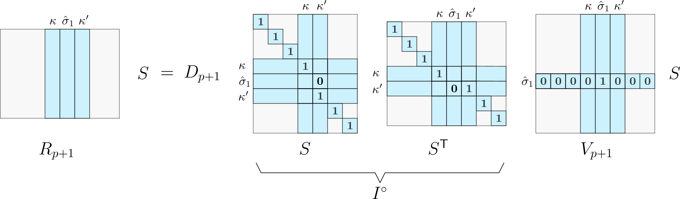
Figure 6: Illustration for the equation \(R_{p+1}S=D_{p+1}SS^\mathsf{T}V_{p+1}S\)..

We summarize the update procedure in 7. Notice that we do not need to actually perform the matrix multiplications as in 21 to get \(R^*_{p+1}\) and \(V^*_{p+1}\): we can simply perform the row addition and row/column removal as needed. The running time is then dominated by the column additions performed. Since there are no more than \(O(m)\) column additions, the time complexity is \(O(m^2)\).
4.3 Update for degree \(p\) and \(p+2\)↩︎
By [obsv:contra-adj-change], \[D^*_{p+2}=T_{p+2}D_{p+2},\] where \(T_{p+2}\) is similar to the matrix \(T\) in 4.2. Let \[R^*_{p+2}=T_{p+2}R_{p+2} \text{ and }V^*_{p+2}=V_{p+2}.\] Then, \[R^*_{p+2}=D^*_{p+2}V^*_{p+2}.\] Notice that there may be two columns in \(R^*_{p+2}\) having the same pivot, and we perform the cascade sum on \(R^*_{p+2}\) and \(V^*_{p+2}\) as in 4.2 to make the pivots distinct.
To see the update for degree \(p\), first notice that \(\partial\sigma_1=\partial\sigma_2\) because there are no insertions and deletions in between the two arrows \(K_{i-1}\xhookleftarrow{\;\sigma\;} K_i \xhookrightarrow{\;\sigma\;} K_{i+1}\) in \(\mathcal{F}\). Then, \(\sigma_2\) is a positive cell in \({\mathcal{F}_\mathrm{nz}}\), where \(\sigma_1+\sigma_2\) is a cycle created by \(\sigma_2\). We then have \({R_{p}}[\cdot,{\sigma}_2]=0\). So we only need to add \({V_{p}}[\cdot,{\sigma}_2]\) to any other \({V_{p}}[\cdot,\kappa]\) with \({V_{p}}[{\sigma}_2,\kappa]\neq 0\), as done similarly in Step I in 4.2. Moreover, we have \[D^*_{p}=D_{p}S_{p},\] where \(S_{p}\) is similar to the matrix \(S\) in 4.2. Let \[R^*_{p}=R_{p}S_{p}\text{ and } V^*_{p}=S_{p}^\mathsf{T}V_{p}S_{p}.\] We then have \[R^*_{p}=D^*_{p}V^*_{p},\] whose justification is the same as that for 22 given by the proof of [prop:Rx-DxVx]. Notice that columns in \(R^*_{p}\) have distinct pivots.
Since the update presented above is also dominated by the column additions and there are no more than \(O(m)\) of them, the update for degree \(p\) and \(p+2\) also takes \(O(m^2)\) time.
We now conclude:
Theorem 2. For an outward contraction operation, given a reduced decomposition \(R_{q}=D_{q}V_{q}\) for \({\mathcal{F}_\mathrm{nz}}\) for each \(q\), one can obtain a reduced decomposition \(R^*_{q}=D^*_{q}V^*_{q}\) for \(\mathcal{F}^*_\mathrm{nz}\) for each \(q\) in \(O(m^2)\) time.
Proof. We have justified the time complexity of the algorithms presented. The correctness of the update follows from the fact that the decomposition \(R^*_{q}=D^*_{q}V^*_{q}\) we maintain is always valid at each step (e.g., we only perform left-to-right column additions) and is reduced at the end. ◻
5 Outward expansion↩︎
We present in this section the update algorithm for outward expansion, which is the inverse operation of outward contraction. Throughout the section, as in 14 , let \(\mathcal{F}^*\) be the filtration before the expansion, and \(\mathcal{F}\), the filtration after. We have that the change from \(D^*_q\) to \(D_q\) for each \(q\) is also the inverse of the change from \(D_q\) to \(D^*_q\), as in [obsv:contra-adj-change], e.g., we still have \(D^*_{p+1}=TD_{p+1}S\).
5.1 Update for degree \(p+1\)↩︎
We describe in detail the update for degree \(p+1\), i.e., given a reduced decomposition \[\label{eqn:exp-given-pplus1} R^*_{p+1}=D^*_{p+1}V^*_{p+1}\tag{23}\] for \(\mathcal{F}^*_\mathrm{nz}\), we find the corresponding decomposition for \({\mathcal{F}_\mathrm{nz}}\). The updates for the degrees \(p\), \(p+2\) are briefly described in 5.2.
Notice that the update for outward expansion is not a simple “inverse” of the update for outward contraction. For example, while adding rows \({D_{p+1}}[\sigma_1,\cdot]\), \({D_{p+1}}[\sigma_2,\cdot]\) to form the row \({D^*_{p+1}}[\sigma_0,\cdot]\) can be written as a left multiplication by \(T\), we cannot do so for the “splitting” of non-zero entries in \({D^*_{p+1}}[\sigma_0,\cdot]\) to get the rows \({D_{p+1}}[\sigma_1,\cdot]\), \({D_{p+1}}[\sigma_2,\cdot]\).
To perform the update, first let \(D'_{p+1}\) be the matrix derived from \(D^*_{p+1}\) by “splitting” the non-zero entries in \({D^*_{p+1}}[\sigma_0,\cdot]\) to form the rows of \(\sigma_1\), \(\sigma_2\), without adding the column of \(\hat{\sigma}_1\). In other words, \(D'_{p+1}:=D_{p+1}S\); see 4. Now, suppose that we are given the following reduced decomposition \[\label{sec:decomp-prime} R'_{p+1}=D'_{p+1}V'_{p+1},\tag{24}\] where \(V'_{p+1}\) has the same dimension as \(V^*_{p+1}\). Then, we can easily obtain a reduced decomposition \(R_{p+1}=D_{p+1}V_{p+1}\) in \(O(m^2)\) time as follows: (1) let \(V_{p+1}\) be derived from \(V'_{p+1}\) by appending a new column that represents a chain containing the single cell \(\hat{\sigma}_1\), and let \(R_{p+1}\) be derived from \(R'_{p+1}\) by appending \(\partial\hat{\sigma}_1\); (2) perform a single iteration of the left-to-right persistence reduction [15] to make \(R_{p+1}\) reduced; (3) using the algorithm in [1], perform \(O(m)\) transpositions to place the columns of \(\hat{\sigma}_1\) in the right place in \(R_{p+1}\) and \(V_{p+1}\), with each transposition taking \(O(m)\) time.
The rest of the subsection focuses on obtaining a reduced decomposition as in 24 from the one in 23 . Since columns in \(D^*_{p+1}\) and \(D'_{p+1}\) have a one-to-one correspondence, let \(V'_{p+1}=V^*_{p+1}\). We “recompute” the boundaries of columns in \(V'_{p+1}\) by letting \(R'_{p+1}=D'_{p+1}V'_{p+1}\). We then have:
For each \((p+1)\)-cell \(\kappa\) in \(\mathcal{F}^*_\mathrm{nz}\), one of the following holds concerning the change from the column \({R^*_{p+1}}[\cdot,\kappa]\) to the column \({R'_{p+1}}[\cdot,\kappa]\):
Case 1: \({R^*_{p+1}}[\sigma_0,\kappa]=0\); \({R'_{p+1}}[\sigma_1,\kappa]=0\) and \({R'_{p+1}}[\sigma_2,\kappa]=0\).
Case 2: \({R^*_{p+1}}[\sigma_0,\kappa]=0\); \({R'_{p+1}}[\sigma_1,\kappa]=1\) and \({R'_{p+1}}[\sigma_2,\kappa]=1\).
Case 3: \({R^*_{p+1}}[\sigma_0,\kappa]=1\); \({R'_{p+1}}[\sigma_1,\kappa]=1\) and \({R'_{p+1}}[\sigma_2,\kappa]=0\).
Case 4: \({R^*_{p+1}}[\sigma_0,\kappa]=1\); \({R'_{p+1}}[\sigma_1,\kappa]=0\) and \({R'_{p+1}}[\sigma_2,\kappa]=1\).
All other entries in the two columns are the same.
Proof. Suppose that \({R^*_{p+1}}[\sigma_0,\kappa]=0\). Then, \(\sigma_0\) is a face of even \((p+1)\)-cells in the chain \({V^*_{p+1}}[\cdot,\kappa]\). Notice that these \((p+1)\)-cells either have \(\sigma_1\) or \(\sigma_2\) as a \(p\)-face in \({\mathcal{F}_\mathrm{nz}}\). Then, either both \(\sigma_1\), \(\sigma_2\) are faces of even \((p+1)\)-cells in \({V'_{p+1}}[\cdot,\kappa]={V^*_{p+1}}[\cdot,\kappa]\) (Case 1) or both are faces of odd \((p+1)\)-cells in \({V'_{p+1}}[\cdot,\kappa]\) (Case 2). It is also not hard to see Case 3 and 4 when \(\sigma_0\) is a face of odd \((p+1)\)-cells in \({V^*_{p+1}}[\cdot,\kappa]\). ◻
For each \((p+1)\)-cell \(\kappa\) in \(\mathcal{F}^*_\mathrm{nz}\), \(\mathrm{piv}({R^*_{p+1}}[\cdot,\kappa])\neq\mathrm{piv}({R'_{p+1}}[\cdot,\kappa])\) if and only if \(\mathrm{piv}({R'_{p+1}}[\cdot,\kappa])=\sigma_2\).
Proof. Suppose that \(\mathrm{piv}({R^*_{p+1}}[\cdot,\kappa])\neq\mathrm{piv}({R'_{p+1}}[\cdot,\kappa])\). Then, either Case 2 or Case 4 in [obsv:col-change] happens because the other cases cannot make the pivot change. If \(\mathrm{piv}({R^*_{p+1}}[\cdot,\kappa])>\sigma_2\) (here we naturally consider the \(p\)-cell \(\mathrm{piv}({R^*_{p+1}}[\cdot,\kappa])\) in \(\mathcal{F}^*_\mathrm{nz}\) as a \(p\)-cell in \({\mathcal{F}_\mathrm{nz}}\)), then \(\mathrm{piv}({R^*_{p+1}}[\cdot,\kappa])=\mathrm{piv}({R'_{p+1}}[\cdot,\kappa])\). So we have \(\mathrm{piv}({R^*_{p+1}}[\cdot,\kappa])<\sigma_2\), which implies that \(\mathrm{piv}({R'_{p+1}}[\cdot,\kappa])=\sigma_2\).
Now suppose that \(\mathrm{piv}({R'_{p+1}}[\cdot,\kappa])=\sigma_2\). Then, \(\mathrm{piv}({R^*_{p+1}}[\cdot,\kappa])\neq\mathrm{piv}({R'_{p+1}}[\cdot,\kappa])\) since \(\mathrm{piv}({R^*_{p+1}}[\cdot,\kappa])\neq\sigma_2\). ◻
For any \((p+1)\)-cells \(\kappa\), \(\nu\) in \(\mathcal{F}^*_\mathrm{nz}\) with \(\mathrm{piv}({R'_{p+1}}[\cdot,\kappa])=\mathrm{piv}({R'_{p+1}}[\cdot,\nu])=\sigma_2\), one has \(\mathrm{piv}({R^*_{p+1}}[\cdot,\kappa]+{R^*_{p+1}}[\cdot,\nu])=\mathrm{piv}({R'_{p+1}}[\cdot,\kappa]+{R'_{p+1}}[\cdot,\nu])\).
Proof. Since \(\mathrm{piv}({R'_{p+1}}[\cdot,\kappa])=\mathrm{piv}({R'_{p+1}}[\cdot,\nu])=\sigma_2\), the columns of \(\kappa\) (resp.\(\nu\)) in \(R^*_{p+1}\) and \(R'_{p+1}\) fall in either Case 2 or 4 in [obsv:col-change]. Denote \({R^*_{p+1}}[\cdot,\kappa]+{R^*_{p+1}}[\cdot,\nu]\) as \(\mathrm{col}_1\) and \({R'_{p+1}}[\cdot,\kappa]+{R'_{p+1}}[\cdot,\nu]\) as \(\mathrm{col}_2\). We then have \(\mathrm{col}_1[\sigma_0]=\mathrm{col}_2[\sigma_1]\), which can be verified by a case analysis of the different values of \({R^*_{p+1}}[\sigma_0,\kappa]\), \({R^*_{p+1}}[\sigma_0,\nu]\), \({R'_{p+1}}[\sigma_1,\kappa]\), and \({R'_{p+1}}[\sigma_1,\nu]\). We omit the case analysis. Since \(\mathrm{col}_2[\sigma_2]=0\) and the other entries of \(\mathrm{col}_1\), \(\mathrm{col}_2\) are the same, we have \(\mathrm{piv}(\mathrm{col}_1)=\mathrm{piv}(\mathrm{col}_1)\). ◻
[prop:col-piv] characterizes those columns whose pivots change from \(R^*_{p+1}\) to \(R'_{p+1}\). [prop:recov-piv] indicates that summing two such columns in \(R'_{p+1}\) “recovers” pivot of the sum in \(R^*_{p+1}\). Since \(R^*_{p+1}\) have distinct pivots, we utilize the above facts to guide our update to make \(R'_{p+1}\) reduced. We then have the following steps.
Step 1: While there are two columns \({R'_{p+1}}[\cdot,\kappa]\) and \({R'_{p+1}}[\cdot,\nu]\), \(\kappa<\nu\), with pivots being \(\sigma_2\) such that \[\mathrm{piv}({R^*_{p+1}}[\cdot,\kappa])<\mathrm{piv}({R^*_{p+1}}[\cdot,\nu]),\] add \({R'_{p+1}}[\cdot,\kappa]\) to \({R'_{p+1}}[\cdot,\nu]\) and \({V'_{p+1}}[\cdot,\kappa]\) to \({V'_{p+1}}[\cdot,\nu]\). After this, \({R'_{p+1}}[\cdot,\nu]\) “regains” its old (unique) pivot in \({R^*_{p+1}}[\cdot,\nu]\), i.e., \(\mathrm{piv}({R'_{p+1}}[\cdot,\nu])=\mathrm{piv}({R^*_{p+1}}[\cdot,\nu])\), due to [prop:col-piv] and the fact that \(\mathrm{piv}({R^*_{p+1}}[\cdot,\kappa])<\mathrm{piv}({R^*_{p+1}}[\cdot,\nu])\)
Step 2: Let \[{R'_{p+1}}[\cdot,\kappa_1],\ldots,{R'_{p+1}}[\cdot,\kappa_\ell]\] be all columns in \(R'_{p+1}\) whose pivots are still \(\sigma_2\), where \[\kappa_1<\cdots<\kappa_\ell.\] We have \[\mathrm{piv}({R^*_{p+1}}[\cdot,\kappa_1])>\cdots>\mathrm{piv}({R^*_{p+1}}[\cdot,\kappa_\ell]),\] and specifically \(\kappa_1,\ldots,\kappa_\ell\) are at the Pareto front of the partial order defined by the order of column indices and the order of pivots in \(R^*_{p+1}\).
We then perform the following update:
- For \(j=\ell,\ell-1,\ldots,2\), add \({R'_{p+1}}[\cdot,\kappa_{j-1}]\) to \({R'_{p+1}}[\cdot,\kappa_j]\) and \({V'_{p+1}}[\cdot,\kappa_{j-1}]\) to \({V'_{p+1}}[\cdot,\kappa_j]\).
After this, each \({R'_{p+1}}[\cdot,\kappa_{j}]\) with \(j>1\) gets the pivot of \({R^*_{p+1}}[\cdot,\kappa_{j-1}]\) because \(\mathrm{piv}({R^*_{p+1}}[\cdot,\kappa_{j-1}])>\mathrm{piv}({R^*_{p+1}}[\cdot,\kappa_{j}])\). Also, \({R'_{p+1}}[\cdot,\kappa_{1}]\) has \(\sigma_2\) as pivot. Hence, columns in \(R'_{p+1}\) now have distinct pivots.
We summarize the update procedure in 8. Since no more than \(O(m)\) column additions are performed, the time complexity is \(O(m^2)\).
5.2 Update for degree \(p\) and \(p+2\)↩︎
To obtain \(R_{p}=D_{p}V_{p}\), one way is to use the approach described at the beginning of 5.1, that is, to append \(\partial\sigma_2\) and \(\sigma_2\) to \(R^*_{p}\) and \(V^*_{p}\), respectively, and to perform \(O(m)\) transpositions to place the two new columns in the correct positions. However, this is an overkill: since \(\partial\sigma_1=\partial\sigma_2\) (see 4.3), inserting \(\sigma_2\) in \({\mathcal{F}_\mathrm{nz}}\) always creates a new cycle \(\sigma_1+\sigma_2\). Hence, we only need to add a column \(0\) and a column \(\sigma_1+\sigma_2\) to \(R^*_{p}\) and \(V^*_{p}\), respectively, at the appropriate place for \(\sigma_2\), which finishes the update for degree \(p\).
For degree \(p+2\), we notice that the change from \(D^*_{p+2}\) to \(D_{p+2}\) is just the “splitting” of \({D^*_{p+2}}[\hat{\sigma}_0,\cdot]\) to get \({D_{p+2}}[\hat{\sigma}_2,\cdot]\) and \({D_{p+2}}[\hat{\sigma}_1,\cdot]\). For this, we use the update procedure for obtaining the decomposition in 24 from that in 23 , as described in 5.1.
We now conclude:
Theorem 3. For an outward expansion operation, given a reduced decomposition \(R^*_{q}=D^*_{q}V^*_{q}\) for \(\mathcal{F}^*_\mathrm{nz}\) for each \(q\), one can obtain a reduced decomposition \(R_{q}=D_{q}V_{q}\) for \({\mathcal{F}_\mathrm{nz}}\) for each \(q\) in \(O(m^2)\) time.
6 Conclusion↩︎
In this paper, we propose algorithms for updating zigzag representatives over eight operations making local changes to a zigzag filtration. The update is performed on the \(R=DV\) decomposition for a non-zigzag filtration constructed from the original zigzag filtration. The zigzag representatives can then be obtained based on 1. Complexities for updating the \(R=DV\) decomposition over the operations are summarized as follows:
Forward/backward switch: \(O(m)\);
Inward/outward switch: \(O(1)\);
Inward/outward expansion/contraction: \(O(m^2)\).
The \(R=DV\) decomposition for persistence is not unique [1]. Just like [1], [5], [16], our updates may not produce the same decomposition as the standard reduction [15], and therefore the same representatives. Also, our updates may not preserve the representatives after an update operation and its reversal, just like [1]. It is an interesting open question whether there are efficient algorithms for such updates.
7 Summary of update procedure for degree \(p+1\) for outward contraction↩︎
Given a reduced decomposition \[R_{p+1}=D_{p+1}V_{p+1}\] for \({\mathcal{F}_\mathrm{nz}}\), do the following:
If \({R_{p+1}}[\cdot,\hat{\sigma}_1]=0\): add \({V_{p+1}}[\cdot,\hat{\sigma}_1]\) to any other \({V_{p+1}}[\cdot,\kappa]\) with \({V_{p+1}}[\hat{\sigma}_1,\kappa]\neq 0\).
If \({R_{p+1}}[\cdot,\hat{\sigma}_1]\neq 0\):
While there are two columns \({V_{p+1}}[\cdot,\kappa]\) and \({V_{p+1}}[\cdot,\nu]\), \(\kappa<\nu\), with non-zero entries on \(\hat{\sigma}_1\) such that \[\mathrm{piv}({R_{p+1}}[\cdot,\kappa])<\mathrm{piv}({R_{p+1}}[\cdot,\nu]),\] add \({V_{p+1}}[\cdot,\kappa]\) to \({V_{p+1}}[\cdot,\nu]\) and \({R_{p+1}}[\cdot,\kappa]\) to \({R_{p+1}}[\cdot,\nu]\).
Let \[{V_{p+1}}[\cdot,\kappa_1],\ldots,{V_{p+1}}[\cdot,\kappa_\ell]\] be all columns in \(V_{p+1}\) that still have non-zero entries on \(\hat{\sigma}_1\), where \[\kappa_1=\hat{\sigma}_1<\kappa_2<\cdots<\kappa_\ell.\]
For \(j=\ell,\ell-1,\ldots,2\), add \({R_{p+1}}[\cdot,\kappa_{j-1}]\) to \({R_{p+1}}[\cdot,\kappa_j]\) and \({V_{p+1}}[\cdot,\kappa_{j-1}]\) to \({V_{p+1}}[\cdot,\kappa_j]\).
Let \[R^*_{p+1}=TR_{p+1}S\text{ and }V^*_{p+1}=S^\mathsf{T}V_{p+1}S.\]
While there are two columns \({R^*_{p+1}}[\cdot,\kappa]\) and \({R^*_{p+1}}[\cdot,\nu]\), \(\kappa<\nu\), with the same pivot, add \({R^*_{p+1}}[\cdot,\kappa]\) to \({R^*_{p+1}}[\cdot,\nu]\) and \({V^*_{p+1}}[\cdot,\kappa]\) to \({V^*_{p+1}}[\cdot,\nu]\).
8 Summary of update procedure for degree \(p+1\) for outward expansion↩︎
Given a reduced decomposition \[R^*_{p+1}=D^*_{p+1}V^*_{p+1}\] for \(\mathcal{F}^*_\mathrm{nz}\), do the following:
Let \(V'_{p+1}=V^*_{p+1}\) and \(R'_{p+1}=D'_{p+1}V'_{p+1}\).
While there are two columns \({R'_{p+1}}[\cdot,\kappa]\) and \({R'_{p+1}}[\cdot,\nu]\), \(\kappa<\nu\), with pivots being \(\sigma_2\) such that \[\mathrm{piv}({R^*_{p+1}}[\cdot,\kappa])<\mathrm{piv}({R^*_{p+1}}[\cdot,\nu]),\] add \({R'_{p+1}}[\cdot,\kappa]\) to \({R'_{p+1}}[\cdot,\nu]\) and \({V'_{p+1}}[\cdot,\kappa]\) to \({V'_{p+1}}[\cdot,\nu]\).
Let \({R'_{p+1}}[\cdot,\kappa_1],\ldots,{R'_{p+1}}[\cdot,\kappa_\ell]\) be all columns in \(R'_{p+1}\) whose pivots are still \(\sigma_2\), where \(\kappa_1<\cdots<\kappa_\ell\).
For \(j=\ell,\ell-1,\ldots,2\), add \({R'_{p+1}}[\cdot,\kappa_{j-1}]\) to \({R'_{p+1}}[\cdot,\kappa_j]\) and \({V'_{p+1}}[\cdot,\kappa_{j-1}]\) to \({V'_{p+1}}[\cdot,\kappa_j]\).
Let \(V_{p+1}\) be derived from \(V'_{p+1}\) by appending a new column that represents a chain containing the single cell \(\hat{\sigma}_1\), and let \(R_{p+1}\) be derived from \(R'_{p+1}\) by appending \(\partial\hat{\sigma}_1\).
Perform a single iteration of the left-to-right persistence reduction [15] to make \(R_{p+1}\) reduced.
Using the algorithm in [1], perform \(O(m)\) transpositions to place the columns of \(\hat{\sigma}_1\) in the right place in \(R_{p+1}\) and \(V_{p+1}\).
9 Generalization to arbitrary field coefficients↩︎
We describe the generalization of our update algorithm to coefficients in an arbitrary field \(\Bbbk\). The update for outward contraction in 4 generalizes immediately because it is expressed entirely as matrix multiplications. So we only describe here how to generalize the update for outward expansion, which boils down to adapting [obsv:col-change,prop:recov-piv]. With a general \(\Bbbk\), each cell needs an orientation. While orientations of most cells can be assigned arbitrarily, we have one restriction: since the \(\Delta\)-cells \(\sigma_1\), \(\sigma_2\) have the same set of vertices, let \(\sigma_1\), \(\sigma_2\) have an orientation induced by the same ordering of vertices. We then have:
Let \(\kappa\) be any \((p+1)\)-cell in \(\mathcal{F}^*_\mathrm{nz}\). Then, \({R^*_{p+1}}[\sigma_0,\kappa]={R'_{p+1}}[\sigma_1,\kappa]+{R'_{p+1}}[\sigma_2,\kappa]\), and \({R^*_{p+1}}[\nu,\kappa]={R'_{p+1}}[\nu,\kappa]\) for any other \(p\)-cell \(\nu\).
We omit the proof of [obsv:col-change-adp], which follows the same idea as the proof of [obsv:col-change]. Notice that [prop:col-piv] is still true here.
For any \((p+1)\)-cells \(\kappa\), \(\nu\) in \(\mathcal{F}^*_\mathrm{nz}\) with \(\mathrm{piv}({R'_{p+1}}[\cdot,\kappa])=\mathrm{piv}({R'_{p+1}}[\cdot,\nu])=\sigma_2\), let \(\alpha_2={R'_{p+1}}[\sigma_2,\kappa]\) and \(\gamma_2={R'_{p+1}}[\sigma_2,\nu]\). Then, for \(\mu=-\gamma_2/\alpha_2\), \(\mathrm{piv}(\mu\cdot{R^*_{p+1}}[\cdot,\kappa]+{R^*_{p+1}}[\cdot,\nu])=\mathrm{piv}(\mu\cdot{R'_{p+1}}[\cdot,\kappa]+{R'_{p+1}}[\cdot,\nu])\).
Proof. Let \(\mathrm{col}_1=\mu\cdot{R^*_{p+1}}[\cdot,\kappa]+{R^*_{p+1}}[\cdot,\nu]\) and \(\mathrm{col}_2=\mu\cdot{R'_{p+1}}[\cdot,\kappa]+{R'_{p+1}}[\cdot,\nu]\). Notice that \(\mathrm{col}_2[\sigma_2]=0\) and \(\mathrm{col}_1[\nu]=\mathrm{col}_2[\nu]\) for any \(\nu\not\in\{\sigma_0,\sigma_1,\sigma_2\}\). So we only need to show \(\mathrm{col}_1[\sigma_0]=\mathrm{col}_2[\sigma_1]\). Let \(\alpha_0={R^*_{p+1}}[\sigma_0,\kappa]\), \(\gamma_0={R^*_{p+1}}[\sigma_0,\nu]\), \(\alpha_1={R'_{p+1}}[\sigma_1,\kappa]\), and \(\gamma_1={R'_{p+1}}[\sigma_1,\nu]\). By [obsv:col-change-adp], we have \(\alpha_0=\alpha_1+\alpha_2\) and \(\gamma_0=\gamma_1+\gamma_2\). Then, \[\mathrm{col}_2[\sigma_1]=(-\gamma_2/\alpha_2)\alpha_1+\gamma_1=(1/\alpha_2)(-\alpha_1\gamma_2+\alpha_2\gamma_1).\] Also, \[\begin{align} \mathrm{col}_1[\sigma_0]&=(-\gamma_2/\alpha_2)\alpha_0+\gamma_0=(-\gamma_2/\alpha_2)(\alpha_1+\alpha_2)+\gamma_1+\gamma_2\\ &=(1/\alpha_2)(-\alpha_1\gamma_2-\alpha_2\gamma_2+\alpha_2\gamma_1+\alpha_2\gamma_2)=(1/\alpha_2)(-\alpha_1\gamma_2+\alpha_2\gamma_1)=\mathrm{col}_2[\sigma_1].\qedhere \end{align}\] ◻
We can then perform the update for outward expansion for degree \(p+1\) in 5.1. The generalization to field \(\Bbbk\) for degree \(p\), \(p+2\) also follows.