Loop the Loopies!
July 17, 2026
1 Introduction↩︎
Looped Transformers, first introduced as Universal Transformers [1], have recently re-emerged as a compelling alternative to conventional depth scaling. Rather than stacking distinct layers, they repeatedly apply the same model across recurrent steps, closely connecting this approach to parameter sharing in Transformers [1], [2]. This recurrent approach has shown strong empirical performance across a wide range of domains, including language modeling, algorithmic learning, and abstract reasoning [1], [3]–[12].
A growing body of work suggests that recurrent computation is especially well suited to complex problems. Looped Transformers can outperform vanilla Transformers on in-context learning and data-fitting tasks, and they can implement multi-step gradient descent in context with far fewer parameters [4], [13]–[17]. Studies of looped Transformers have also shown that recurrent computation allows shallow parameterizations to approach the performance of deeper untied models on reasoning tasks [7], [9], [10], [18]. These advantages are particularly visible on abstract reasoning tasks such as ARC-AGI, Sudoku, and Maze, where results from recent recurrent models suggest that recurrence provides a powerful inductive bias for compositional generalization, rule discovery, and inductive reasoning [3], [5], [6].
Recent work has begun scaling looped Transformers to billion-parameter language models. Ouro models scale to 1.4B and 2.6B parameters with four recurrent steps, reporting strong parameter efficiency relative to larger dense baselines [10]. Huginn scales to 3.5B parameters and uses 32 recurrent steps to trade parameters for latent computation [9]. Other systems further study adaptive recurrence, efficient reasoning, memory–compute trade-offs, and scaling laws for stable looped language models [8], [11], [18], [19]. However, these gains expose a fundamental compute-accounting issue: looping a model \(N\) times during pre-training also multiplies pre-training compute by \(N\). Thus, looped Transformers should be compared not only against vanilla Transformers with the same parameter count but also against non-looped models trained under the same pre-training compute budget. This view is consistent with language-model scaling and compute-optimal training analyses, which evaluate quality as a function of parameters, data, and total training FLOPs rather than parameter count alone [19]–[21]. For example, Ouro-2.6B with 4 loops should be compared against a baseline model with a parameter count close to 2.6B × 4 = 10.4B; likewise, after accounting for pre-training compute, Huginn-3.5B with 32 loops should be compared against a much larger 112B-parameter baseline model. This motivates our central question:
Can looped Transformers match or exceed vanilla Transformers
under the same pre-training compute budget?
We answer this question with the Loopie Series: two looped MoE LLMs, Loopie-20B-A2B and Loopie-6B-A0.6B, each trained with two loop steps. Our key idea is the Loopie Recipe, a compute-matched scaling recipe that addresses the main concern for recurrent-depth scaling: under a fixed pre-training compute budget, vanilla parameter scaling can otherwise dominate looping [19], [21]. With a novel post-training method, Loopie develops strong reasoning abilities and achieves frontier-level gold-medal performance on the 2025 IPhO and IMO problems without tools.
Our contributions are threefold:
Compute-matched scaling. We introduce the Loopie Recipe to address the fixed-compute challenge for looped Transformers and validate it through extensive ablations.
Scalable looped MoE models. We demonstrate that looped computation scales to large MoE language models by training Loopie-20B-A2B and Loopie-6B-A0.6B.
Large-scale post-training. We scale Loopie through large-scale post-training, including a novel supervised pre-training stage, it yields strong reasoning abilities and gold-medal performance on the IMO and IPhO.
![Figure 1: Illustration of the contrast between layer-loop and model-loop. The top panel shows layer-loop, the loop schedule adopted by Loopie, in which each Attention/MoE layer is applied recurrently before passing its output to the next layer. We demonstrate that this schedule achieves better performance on MoE backbones while also training more efficiently. The bottom panel shows the traditional whole-model recurrence pattern, which we call model-loop, where the entire layer stack is traversed and then repeated. This pattern is used by prior looped models such as Ouro and Huginn [9], [10].](/article/2607.16051/_pdflatex/mxfwvsck.png "fig:")
2 The Loopie Series↩︎
This section presents the Loopie Series, from its architecture to the evidence for its scalability. We begin by defining Loopie’s layer-loop recurrence pattern and contrasting it with the classic model-loop pattern used in prior looped language models. We then motivate the design under a fixed pre-training compute budget, where models that use recurrent depth must be compared against vanilla Transformers that spend the same compute on ordinary non-recurrent capacity. Building on this motivation, we introduce the Loopie Recipe, a compute-matched scaling recipe for choosing stored width, stored depth, and recurrent depth. We next present the main compute-matched results, examine whether the advantage persists across model scales, and isolate the contribution of the layer-loop pattern through ablations. Finally, we discuss why Loopie uses only two recurrent steps.
2.1 Architecture↩︎
Loopie largely follows the Qwen3-MoE architecture. In particular, its backbone is a decoder-only Mixture-of-Experts Transformer, and its attention mechanism, sparsity pattern, and other architectural details remain the same as those of the Qwen3-MoE family. Detailed architectural specifications are provided in Appendix [arch95details]. The key architectural difference lies in how recurrent computation is applied. Instead of simply repeating the entire model multiple times, Loopie adopts a different recurrence pattern that we call layer-loop.
Prior looped language models, such as Ouro and Huginn [9], [10], mainly use what we call model-loop. In model-loop recurrence, the entire Transformer stack is unrolled recurrently: for a model with three layers and two loop steps, the computation order is \[\text{Layer 1} \rightarrow \text{Layer 2} \rightarrow \text{Layer 3} \rightarrow \text{Layer 1} \rightarrow \text{Layer 2} \rightarrow \text{Layer 3}.\] By contrast, Loopie uses layer-loop, in which each layer is applied recurrently before the computation moves to the next layer. For the same three-layer, two-step example, the computation order becomes \[\text{Layer 1} \rightarrow \text{Layer 1} \rightarrow \text{Layer 2} \rightarrow \text{Layer 2} \rightarrow \text{Layer 3} \rightarrow \text{Layer 3}.\] That is, each block performs local iteration on the hidden states and only then passes the resulting recurrent representation to the next layer. Figure 1 illustrates the difference.
2.2 Why Layer-Loop?↩︎
Layer-loop is not merely a different ordering of recurrent computation; it changes where iterative refinement happens inside the model and therefore affects scaling behavior, execution efficiency, and the nature of parameter sharing across effective depth. We adopt layer-loop because it offers three advantages that are especially important for large-scale pre-training.
2.2.0.1 Better empirical scaling.
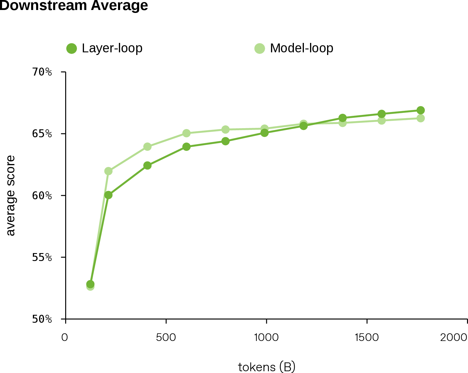
Layer-loop achieves better performance than model-loop in our pre-training experiments. As shown in Figure 2, layer-loop initially trails model-loop slightly on downstream benchmarks. However, it overtakes model-loop after approximately \(1.2\) trillion training tokens and improves more rapidly thereafter. The early advantage of model-loop therefore does not persist as the training budget increases.
2.2.0.2 Infrastructure-friendly execution.
Although layer-loop and model-loop have the same nominal number of layer applications and theoretical FLOPs, layer-loop provides better execution locality. Repeated applications of the same layer are adjacent in both the forward and backward computation graphs, which shortens the reuse distance for parameters and gradient contributions and simplifies activation checkpointing and gradient accumulation, especially under parameter sharding or offloading. This locality is particularly beneficial for pipeline parallelism because all recurrent applications of a layer remain within the same pipeline stage before activations are transferred onward. In contrast, model-loop requires each microbatch to traverse the entire pipeline repeatedly and routes the output of the final stage back to the first stage at each loop boundary, introducing cyclic dependencies that may complicate scheduling, increase communication overhead and the number of pipeline bubbles, and reduce device utilization.
2.2.0.3 Natural parameter-sharing pattern.
For example, consider a 48-layer model such as Qwen3-30B-A3B with two model-loop steps. The third physical layer is applied at effective depths \(3\) and \(48 + 3 = 51\). These two invocations occur after markedly different amounts of preceding computation and therefore receive hidden states at widely separated effective depths. Prior analyses suggest that Transformer representations are organized nonuniformly across depth: lower and final layers can differ substantially from the comparatively homogeneous middle layers, while different linguistic abstractions tend to become most accessible at different stages of the network [22]–[24]. These observations do not directly establish gradient conflict, but they suggest that hidden states at widely separated effective depths need not place identical functional demands on a shared transformation. Thus, model-loop asks a single parameter set to accommodate potentially heterogeneous depth-dependent roles. In contrast, layer-loop reuses a layer at adjacent effective depths, resulting in a more local and potentially more coherent parameter-sharing pattern.
2.3 Motivation↩︎
Despite their conceptual appeal, looped Transformers have historically been studied in settings that do not fully reflect the constraints of modern large-scale language model pre-training. In particular, much of the prior work has focused on dense, weight-shared, or recurrent Transformer variants and has evaluated recurrence primarily as a mechanism for improving parameter efficiency [9], [10]. This leaves two important issues underexplored.
First, modern frontier language models increasingly rely on Mixture-of-Experts architectures, as exemplified by the recent Qwen3, Kimi K2.5, GLM-5, DeepSeek-V4, and MiniMax-M2 model families [25]–[29]. MoE models expand total model capacity while keeping the number of active parameters per token relatively small, making them substantially more favorable than dense models under both training and inference compute constraints [30]–[33]. A practical looped architecture should therefore be compatible with MoE scaling rather than be restricted to dense backbones, because such a restriction would limit its ability to scale to larger model sizes.
Second, pre-training compute is often the dominant constraint in large-model training. It determines how large a model can be, how many tokens it can see, and how many experimental variants can be trained [20], [21]. This creates a key difficulty for looped Transformers: recurrent computation is not free. If a model is looped \(N\) times during pre-training, its training compute is also multiplied by approximately \(N\). Therefore, a looped model should not merely outperform a vanilla Transformer with the same stored parameter count. To justify recurrence as a scaling strategy, it must compete with vanilla Transformers trained under the same pre-training compute budget.
This requirement is challenging. Prior work suggests that, under fixed-FLOP comparisons, a looped model can have less non-recurrent capacity than a standard Transformer baseline [34], [35]. This is consistent with the conventional view that recurrence mainly improves parameter efficiency but not necessarily compute efficiency [2], [36]. As a result, prior looped Transformers have not yet provided a clear path toward flagship models at the trillion-parameter scale with frontier-level performance.
Loopie is designed to address this gap. Our central observation is that recurrence becomes competitive under a fixed compute budget only when it is paired with an appropriate recurrence-width-depth trade-off. We formalize this principle as the Loopie Recipe: rather than treating loops as a direct substitute for additional parameters, one should jointly choose stored width, stored depth, and recurrent depth so that the resulting model maximizes performance under a fixed pre-training compute budget. This changes the role of recurrence from a parameter-saving device into a compute-matched scaling mechanism.
2.4 Loopie Recipe↩︎
We now describe the empirical, hardware-aware scaling procedure used to instantiate Loopie-20B-A2B. Starting from a strong non-recurrent MoE reference, the Loopie Recipe comprises three steps:
(i) constructing a recurrent seed model by halving the number of stored layers;
(ii) executing each stored layer twice using layer-loop; and
(iii) using the resulting memory headroom to double the per-device microbatch size, then reinvesting the measured training efficiency gain into additional model capacity while keeping the optimizer-step time approximately matched to the reference
model.
In this work, we match models by realized pre-training cost rather than by exact theoretical FLOPs. For every comparison, we fix the hardware allocation, sequence length, number of tokens per optimizer step, activation-checkpointing policy, optimizer, and training data. Architectures may use different per-device microbatch sizes according to their measured memory footprints. When the microbatch size is increased, the number of gradient-accumulation steps is reduced proportionally so that the number of tokens per optimizer step remains unchanged.
We select the Loopie configuration whose measured end-to-end optimizer-step time most closely matches the non-recurrent reference. Since both models use the same token budget and number of optimizer updates, this also approximately matches total wall-clock training cost.
The models are not matched by their theoretical FLOP counts. Loopie performs more nominal computation per token, but the additional work is offset by the higher realized efficiency. We refer to this operationally as a compute-matched comparison. Analytical FLOP and memory models are used only to construct and interpret candidate configurations. The final architecture is selected using measured end-to-end training time in Megatron-LM [37].
The measured efficiency gain comes solely from the reduced stored depth, which lowers activation memory and enables us to double the per-device microbatch size while halving the number of gradient-accumulation steps.
2.4.0.1 Activation memory and microbatch efficiency.
Under the checkpointing implementation used in our experiments, all recurrent applications of a stored layer are enclosed in the same checkpointed unit. Consequently, the dominant activation memory term scales with stored depth rather than executed depth. The activation memory \(M_{\mathrm{act}}\) during training scales as [38], [39] \[M_{\mathrm{act}} \propto s\,bDL,\] where \(D\) is the hidden dimension, \(L\) is the number of stored layers, \(b\) is the per-device microbatch size, and \(s\) is the sequence length. The recurrent applications increase the amount of executed computation through the loop count \(R\) but do not introduce \(R\) independently stored sets of layer-boundary activations under this checkpointing scheme.
For a fixed global batch size \(B\), with per-device microbatch size \(b\) and \(g\) gradient-accumulation steps, we have \[g = \frac{B}{b}.\] Reducing \(DL\) creates memory headroom that can be used to increase \(b\). Because the number of gradient-accumulation steps \(g\) is reduced proportionally, the global batch size remains fixed: \[b_{1} = 2b_{0}, \qquad g_1 = \frac{g_0}{2}.\] The larger microbatch exposes more parallel work to each kernel and reduces the number of gradient-accumulation micro-steps required for each optimizer update.
For a fixed architecture, the corresponding microbatch efficiency gain is measured directly as \[S_{\mathrm{mb}} = \frac{ t_{\mathrm{step}}(D,L,R;b,g) }{ t_{\mathrm{step}}(D,L,R;2b,g/2) }.\] This measured quantity is the efficiency factor used by the Loopie Recipe.
We use a Qwen3-like 30B-A3B MoE Transformer [25] as the non-recurrent reference, with \[D_0 = 2048, \qquad L_0 = 48, \qquad R_0 = 1.\] The first step is to construct a recurrent seed model by halving the number of stored layers and setting \(R=2\): \[D = 2048, \qquad L = 24, \qquad R = 2.\] The leading-order pre-training compute [21] scales as \[C(D,L,R) \propto L D^2 R.\] At a fixed width, this transformation preserves the number of Transformer block executions: \[LR = 24\cdot 2 = 48 = L_0R_0,\] and therefore preserves the leading-order Transformer block compute proxy: \[LRD^2 = 24\cdot 2\cdot 2048^2 = 48\cdot 2048^2.\]
At the same per-device microbatch size, the dominant activation memory term is reduced by half: \[\frac{DL}{D_0L_0} = \frac{2048\cdot 24}{2048\cdot 48} = 0.5.\] The recurrent seed model therefore performs approximately the same leading-order Transformer block work as the reference while requiring substantially less memory for stored activations [37], [39].
The second step is to spend the resulting microbatch efficiency on additional model capacity. To satisfy architectural and hardware alignment constraints, we restrict the candidate hidden sizes to multiples of 128. We sweep feasible \((D,L)\) configurations around the recurrent seed model and retain candidates that support a microbatch size twice that of the reference.
Table 1 lists the candidate configurations. We report the normalized leading-order compute proxy: \[\widehat{C} = \frac{LRD^2}{48\cdot 2048^2},\] and the activation memory proxy at the reference microbatch size, \[\widehat{M}_{\mathrm{act}} = \frac{DL}{48\cdot 2048}.\] These quantities are used to describe the candidates, not to predict their final optimizer-step times.
| Configuration | \(D\) | \(L\) | \(R\) | \(\widehat{C}\) | \(\widehat{M}_{\mathrm{act}}\) |
|---|---|---|---|---|---|
| Qwen3 30B-A3B | 2048 | 48 | 1 | \(1.00\times\) | \(1.00\times\) |
| Seed Loopie | 2048 | 24 | 2 | \(1.00\times\) | \(0.50\times\) |
| Loopie candidate 1 | 2176 | 25 | 2 | \(1.18\times\) | \(0.55\times\) |
| Loopie candidate 2 | 2304 | 27 | 2 | \(1.42\times\) | \(0.63\times\) |
| Loopie candidate 3 | 2432 | 28 | 2 | \(1.65\times\) | \(0.69\times\) |
We conduct large-scale benchmarking of each candidate configuration in Megatron-LM, following the matching protocol described above. For the reference model and each candidate model, we jointly search over tensor parallelism, expert parallelism, and microbatch size. We then select the candidate whose measured optimizer-step time is closest to that of the non-recurrent reference model: \[D_1 = 2304, \qquad L_1 = 27, \qquad R_1 = 2,\] which defines Loopie-20B-A2B.
At the reference per-device microbatch size, the dominant activation memory proxy of Loopie-20B-A2B relative to the reference is \[\frac{D_1L_1}{D_0L_0} = \frac{2304\cdot 27}{2048\cdot 48} \approx 0.633.\] This expression is a scaling proxy rather than an exact peak-memory equation. Candidate feasibility is therefore determined using the measured full memory footprint, which also includes parameters, optimizer states, temporary buffers, and communication workspaces. The measured memory profile of Loopie-20B-A2B permits the per-device microbatch size to be doubled: \[b_{1} = 2b_{0}, \qquad g_1 = \frac{g_0}{2}.\] This leaves the number of tokens per optimizer step unchanged. The selected model has a normalized leading-order Transformer block compute proxy of \[\frac{\widehat{C}_1}{\widehat{C}_0} = \frac{ 27\cdot 2\cdot 2304^2 }{ 48\cdot 2048^2 } \approx 1.424.\] Loopie-20B-A2B matches the reference optimizer-step time only after changing the schedule from \((b_0, g_0)\) to \((2b_0, g_0/2)\); thus, the measured efficiency gain is entirely attributable to the doubled microbatch size.
The compute-matching criterion is therefore the directly measured relation: \[t_{\mathrm{step}} \left( D_1,L_1,R_1; 2b_{0},g_0/2 \right) \approx t_{\mathrm{step}} \left( D_0,L_0,R_0; b_{0},g_0 \right),\] rather than an analytical prediction based on \(\widehat{C}\). The leading-order compute proxy omits lower-order operators, routing and communication costs, optimizer overhead, kernel-launch overhead, and the effect of the microbatch schedule on realized hardware utilization. It is therefore used to characterize nominal work, not to replace end-to-end timing. We evaluated the Loopie Recipe across multiple GPU platforms and observed consistent infrastructure-level gains.
The Loopie Recipe therefore does not claim equality in analytical FLOP estimates. It uses layer-loop recurrence to reduce the stored memory footprint, converts the resulting memory headroom into a doubled per-device microbatch size, spends the measured microbatch efficiency gain on additional model capacity, and selects the final architecture using measured end-to-end optimizer-step time.
2.5 Results↩︎
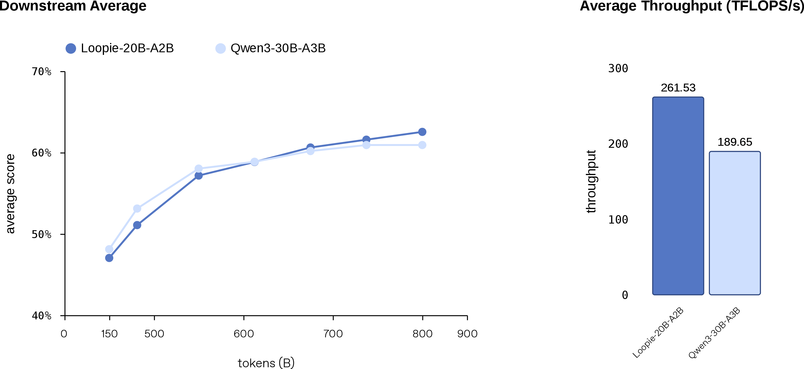
To test this principle, we compare Loopie against a strong non-recurrent baseline based on the Qwen3-MoE design. Specifically, we train a vanilla 30B-A3B MoE Transformer with a Qwen3-like architecture on 800 billion tokens under the same pre-training compute budget used for Loopie-20B-A2B. As shown in Figure 3, Loopie initially lags behind the larger vanilla baseline during the early phase of training. However, after roughly 600 billion tokens of pre-training, Loopie-20B-A2B overtakes the compute-matched baseline and maintains a consistent advantage thereafter. This result suggests that, with the right scaling recipe, looped MoE models can achieve stronger final performance by using recurrent computation than by allocating the same compute to a larger vanilla Transformer.
2.6 Scalability↩︎
A practical recurrent architecture should not only outperform a single compute-matched baseline but also remain effective as the model is scaled. Many architectural ideas show promising results at one small scale yet fail at larger scales for various reasons. We therefore evaluate whether the Loopie design preserves its advantage across a sequence of increasingly large pre-training runs.
We construct a scaling ladder consisting of four non-recurrent MoE baselines and four compute-matched Loopie models. Each Loopie model is obtained by transforming a non-recurrent MoE baseline using the Loopie Recipe. At each rung, the Loopie model uses two layer-loop steps, and its stored width and depth are chosen according to the same compute-matched principle described in Section 2.4. The goal of this ladder is not to match the stored parameter count but to match the effective pre-training compute of the corresponding vanilla baseline. Thus, the Loopie models contain fewer stored parameters while using recurrence to increase effective depth.
For each reference model, we train on a token count equal to 1000× its active MoE parameter count, ensuring that each model is sufficiently overtrained and that its downstream metrics have largely stabilized. We use the same token budget for the corresponding Loopie models, even though these models have fewer active parameters.
For the smallest rung, we train the 0.15B vanilla baseline and its compute-matched 0.10B Loopie counterpart on 150B tokens, placing the models in a heavily overtrained regime relative to standard Chinchilla-style compute-optimal prescriptions. For the 0.25B and 0.50B rungs, we train on 250B and 500B tokens, respectively. For the 1B vanilla baseline and the corresponding 0.70B Loopie model, we also train on 500B tokens due to limited compute. The architectural details for this scaling ladder are provided in Appendix Table 4.
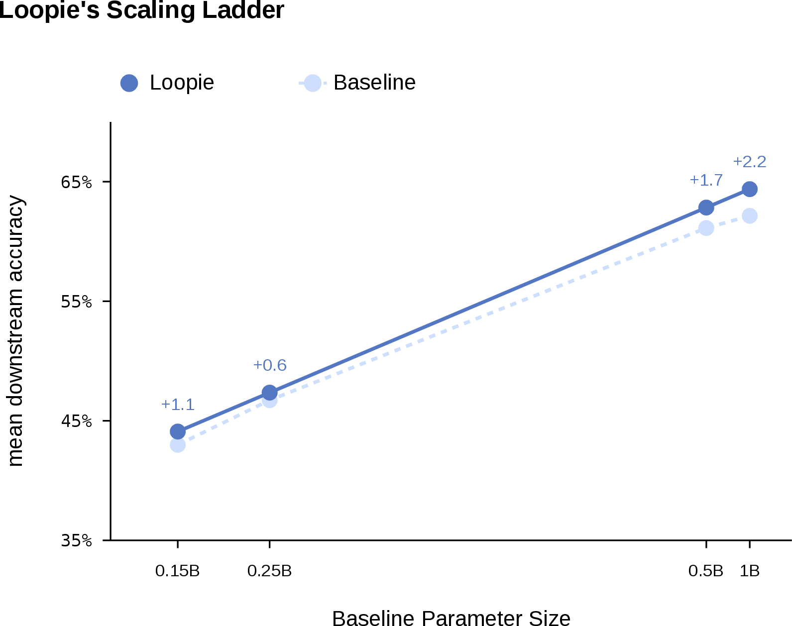
Figure 4 summarizes the resulting scaling behavior. Across all four rungs, Loopie consistently outperforms its compute-matched vanilla counterpart. More importantly, the gap does not vanish as model size increases. This suggests that Loopie’s advantage persists across a meaningful scaling ladder rather than being merely a small-model artifact. The result supports the central design hypothesis of the Loopie Series: recurrent layer-loop computation can be converted into scalable modeling gains when stored width, stored depth, and recurrent depth are jointly chosen under a fixed compute budget.
Taken together, the scaling ladder provides evidence that Loopie remains effective beyond an isolated compute-matched comparison. As the baseline parameter count grows from 0.15B to 1B, Loopie models continue to deliver stronger downstream accuracy under matched pre-training budgets. This behavior is important for large-scale deployment: it indicates that the layer-loop design and the Loopie Recipe are compatible with progressive scaling rather than being limited to a narrow model-size regime.
2.7 Ablations↩︎

In addition to comparing Loopie against a compute-matched vanilla MoE baseline, we further isolate the contribution of the layer-loop recurrence schedule. To do so, we conduct a controlled experiment by training a 6B-A0.6B MoE model with the same backbone, optimizer, data mixture, and token budget as Loopie-6B-A0.6B but with the layer-loop pattern removed. This ablated model therefore preserves the overall looped computation budget while testing whether the ordering of recurrent computation is itself important.
Figure 5 shows the resulting average score across eight downstream benchmarks. The layer-loop pattern substantially improves downstream performance relative to the matched ablation. Importantly, because neither the number of active parameters nor the overall computation budget increases, the improvement cannot simply be attributed to additional computation.
This result supports the architectural choice made in Loopie. While recurrence increases effective depth, the way recurrence is scheduled matters: naively looping computation is insufficient to achieve high compute efficiency. These ablations suggest that Loopie’s gains arise not only from using recurrence but from using recurrence in a form that is aligned with the hierarchical structure of Transformer representations.
2.8 Why Only Two Loop Steps?↩︎
Many recurrent language model designs use substantially deeper unrolling. For example, prior looped or latent-recurrent models often use 4, 16, or even more than 30 recurrent steps [9], [10]. These settings are useful for studying recurrence as a general mechanism for iterative computation. Loopie targets a different regime: large-scale language model pre-training under a fixed compute budget. In this regime, the number of loop steps is not merely an architectural hyperparameter; it is a direct allocation of pre-training FLOPs.
At a fixed stored parameter count and a fixed number of optimizer steps, increasing the number of loop steps usually improves the training curve. However, this comparison is not compute-matched. For a model with \(R\) loop steps, the per-token training cost scales approximately linearly with \(R\), up to MoE routing and implementation constants: \[\mathcal{C}(D,L,R) \propto L D^2 R .\] Under the same pre-training budget, the model must either be trained on fewer tokens, use a smaller stored architecture, or be compared against a stronger non-recurrent model that spends the same compute on ordinary Transformer capacity. The relevant question is thus not whether a model with \(R=4\) outperforms one with \(R=2\) at the same stored size but whether the marginal gain from additional recurrence exceeds the gain that could be obtained by reallocating the same FLOPs to width, depth, or data.
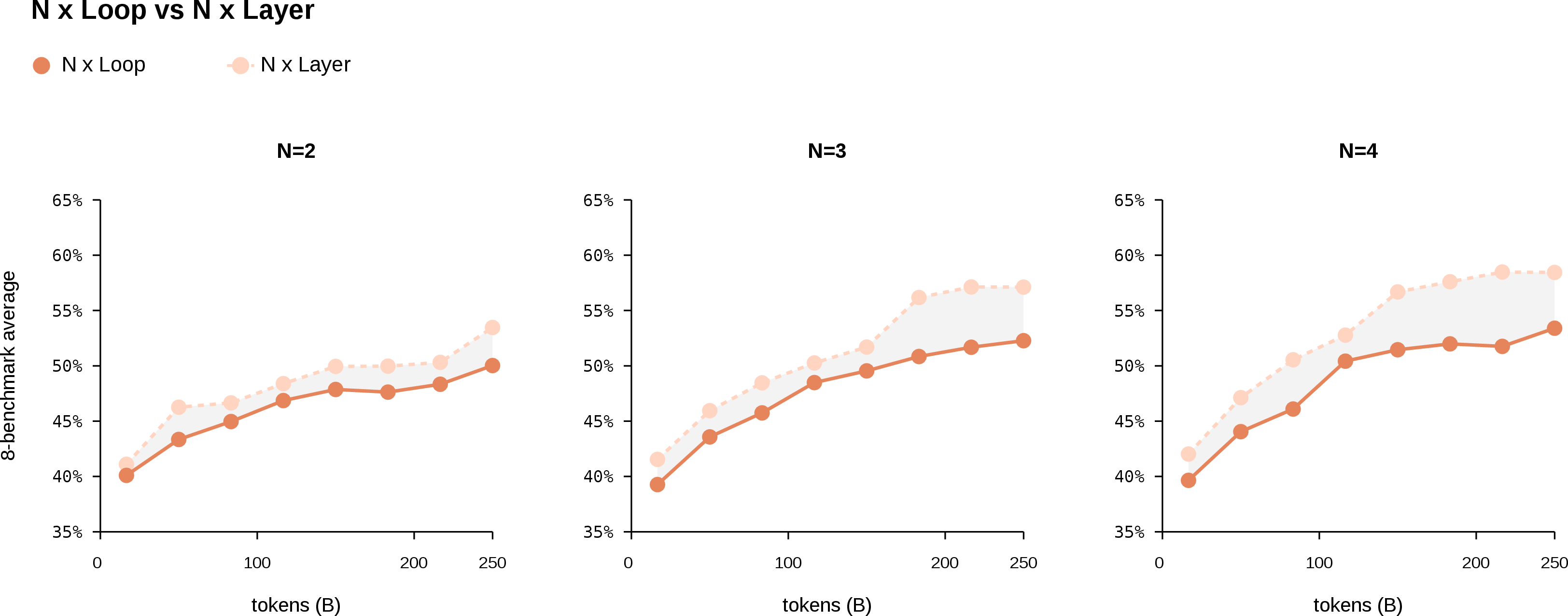
Our loop-count sweep suggests that this marginal return decays rapidly in the large-scale pre-training regime. To isolate whether the gain comes from recurrence rather than simply adding more non-shared layers, we compare a model that uses \(N\times\) layer-loop steps with one that has \(N\times\) as many stored layers, while holding all other architectural details fixed. Figure 6 reports the average score across eight downstream benchmarks after the models are trained on 250B tokens. The shaded gray region highlights the performance gap between the \(N\times\) layer baseline and the \(N\times\) loop model. For the \(2\times\) comparison, we use a \(2\times\) stored-layer model only as a conservative proxy for the previous compute-matched setting. Because this model is very small, with only 0.25B active parameters, precise compute matching is difficult under multiple practical constraints, so the actual training compute of the \(2\times\) layer baseline is substantially higher than that of the \(2\times\) loop model. Thus, the figure should not be read as evidence that \(2\times\) looping is dominated by \(2\times\) layer scaling; rather, it shows that, when comparing \(N\times\) looping against \(N\times\) stored-layer scaling, the marginal benefit of recurrence is largest at \(R=2\).
We therefore choose \(R=2\) for the Loopie Series. This is the smallest nontrivial recurrent setting: each layer performs one ordinary transformation followed by one local refinement step before passing its representation to the next layer. This permits recurrence to change the computation qualitatively while keeping the compute multiplier small enough for scalable pre-training. It also preserves training throughput and makes the comparison against Qwen3-like vanilla MoE baselines stringent: Loopie must outperform these baselines not by using a large amount of extra recurrent computation but by using a small amount of recurrence more effectively.
This choice should not be interpreted as claiming that larger loop counts are ineffective in isolation. Larger \(R\) may be useful in settings where inference-time computation is cheap, where adaptive computation is available, or where the goal is to study recurrent reasoning rather than pre-training efficiency. For frontier-scale pre-training, however, the dominant constraint is total compute. Under this constraint, \(R=2\) provides the best trade-off we observe between iterative refinement, throughput, and compute-matched scaling.
3 Pre-Training↩︎
We pre-train Loopie models in two stages. In the first stage, we perform large-scale pre-training from scratch on 3T tokens. In the second stage, we conduct high-quality data annealing using 1.26T tokens, with an emphasis on high-quality synthetic, STEM, code, mathematical reasoning, and web data. All Loopie models use the tokenizer from the Qwen3 model family [25]. We conduct all pre-training using the Megatron-LM [37] framework.
3.1 Evaluation↩︎
We evaluate the pre-trained checkpoints using the LM Evaluation Harness framework [40]. For all experiments in Section 2, we report the mean score across the following eight benchmarks: ARC-Challenge [41], ARC-Easy [41], BoolQ [42], CommonsenseQA [43], HellaSwag [44], MMLU [45], OpenBookQA [46], and WinoGrande [47].
3.2 Initialization↩︎
Let \(d\) denote the model width. We initialize the token embedding matrix \(E\) and the language-modeling head \(W_{\mathrm{lm}}\)—or the shared embedding/unembedding matrix when weight tying is used—as \(E_{ij},(W_{\mathrm{lm}})_{ij}\sim\mathcal{N}(0,d^{-1})\). On the input side, the looked-up embeddings are multiplied by \(\sqrt d\) before entering the residual stream, so that the embedding shortcut has \(O(1)\) activation scale, while the same \(d^{-1}\) variance ensures that the initial logits \(h^\top w\) have \(O(1)\) variance for normalized hidden states [48], [49]. For hidden-to-hidden parameters inside Transformer blocks, including attention projections and feed-forward layers, we use SmallInit: \[W_{ij}\sim \mathcal{N}\!\left(0,\frac{2}{5d}\right), \qquad \operatorname{std}(W)=\frac{1}{\sqrt{2.5d}}.\] This scale corresponds to Xavier fan-in/fan-out initialization for a Transformer FFN with an expansion ratio of \(4\), since \(d_{\rm in}+d_{\rm out} =d+4d=5d\). We also apply this scale to attention projections to reduce the scale of residual-branch sub-layers [50], [51]. Thus, we use \(d^{-1/2}\) for embeddings/unembeddings, which determine the shortcut and logit scales, but \((2.5d)^{-1/2}\) for block sub-layers, whose Jacobians should remain small for stable pre-training [49].
3.3 Learning Schedule↩︎
We optimize all models with AdamW [52], [53]. We set the peak learning rate to \(5\times 10^{-4}\) for Loopie-6B-A0.6B and \(3\times 10^{-4}\) for Loopie-20B-A2B. We set the AdamW hyperparameters to \(\beta_1=0.9\), \(\beta_2=0.95\), and \(\epsilon=10^{-15}\), use a weight decay of \(0.1\), and apply global gradient-norm clipping at \(1.0\). We use a warmup-stable-only learning-rate schedule. After a specified number of warmup steps—6,000 steps for Loopie-20B-A2B and 2,000 steps for Loopie-6B-A0.6B—the learning rate reaches its peak value and then remains constant without decay. This decay-free stable phase keeps the effective update scale high after warmup, avoiding the diminished influence of late-stage high-quality data that can occur under annealed schedules [54]–[56]. We also use a constant learning rate during the high-quality annealing phase in Stage 2 to maximize learning from the highest-quality annealing data [55]. The global batch size is 1024, and the sequence length is 8192.
3.4 Stage 1: Multi-Epoch High-Quality Pre-Training↩︎
In Stage 1, we train both Loopie-20B-A2B and Loopie-6B-A0.6B on Nemotron-CC-v2-HQ [57], a high-quality subset of Nemotron-CC. The corpus contains approximately 570B unique tokens, and we train for four epochs, totaling approximately 2.28T training tokens. This design is motivated by our prior observation that repeated training on high-quality data can be more effective than single-pass training on a larger corpus of lower average quality [58].
3.5 Stage 2: High-Quality Annealing↩︎
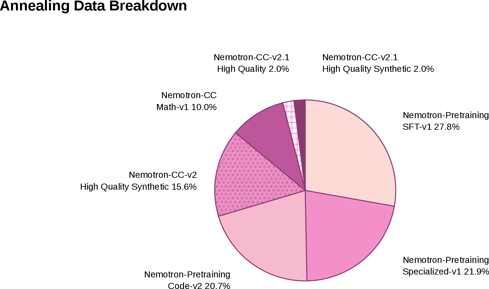
In Stage 2, we construct a high-quality annealing mixture from Nemotron pre-training datasets. The resulting pool contains approximately 1.26T tokens. The mixture combines high-quality SFT-style data, synthetic reasoning data, code data, synthetic web data, and math data. In total, the pool contains approximately 1263B tokens: 351B from Nemotron-pre-training-SFT-v1 (27.8%), 277B from Nemotron-pre-training-Specialized-v1 (21.9%), 262B from a 60% sample of Nemotron-pre-training-Code-v2 (20.7%), 197B from a 16% sample of Nemotron-CC-v2-HQ-Synthetic (15.6%), 126B from Nemotron-CC-Math-v1 with quality scores \(\geq 4\) (10.0%), 25B from Nemotron-CC-v2.1-HQ (2.0%), and 25B from Nemotron-CC-v2.1-HQ-Synthetic (2.0%). Figure 7 visualizes these relative proportions.
3.5.0.1 Nemotron-pre-training-SFT-v1.
We include approximately 351B tokens from Nemotron-pre-training-SFT-v1, a diverse SFT-style dataset of synthetic and curated examples spanning STEM, academic, code, mathematics, and reasoning domains, with multilingual coverage. Its STEM component is expanded from high-quality math and science seeds through iterative generation with Qwen3 and DeepSeek models, producing harder and more varied questions with solutions. The dataset also contains academic question-answer pairs synthesized from undergraduate- and graduate-level texts, as well as MMLU-style general QA and fundamental reasoning data.
3.5.0.2 Nemotron-pre-training-Specialized-v1.
We include approximately 277B tokens from Nemotron-pre-training-Specialized-v1, which comprises synthetic data for STEM reasoning, scientific coding, and cross-domain coding, as well as synthetic Wikipedia data and synthetic mathematics textbook data. The STEM reasoning component includes reasoning question-answer demonstrations generated from advanced scientific seed documents, while the scientific coding and cross-domain coding subsets introduce graduate- or research-level programming tasks with structured solutions. This data is intended to strengthen scientific reasoning, mathematical abstraction, and code generation during annealing.
3.5.0.3 Nemotron-pre-training-Code-v2.
We randomly sample 60% of Nemotron-pre-training-Code-v2, yielding approximately 262B tokens. This dataset combines recent GitHub source code, synthetic code-grounded question-answer data, student-teacher dialogues, code-review dialogues, and LLM-rewritten or transpiled source code. The rewriting and transpilation components are designed to improve downstream code generation by increasing stylistic diversity and exposing the model to semantically equivalent code variants.
3.5.0.4 High-quality synthetic web data.
We randomly sample 16% of Nemotron-CC-v2-High-Quality-Synthetic, yielding approximately 197B tokens. This dataset is derived from Nemotron-CC-v2 and contains English web-crawl documents augmented through synthetic rephrasing with Qwen3-30B-A3B. We further include 25B tokens from Nemotron-CC-v2.1-High-Quality-Synthetic, which extends the synthetic high-quality web corpus with newer Common Crawl snapshots and additional rephrased medium- to high-quality documents.
3.5.0.5 High-quality web data.
We include approximately 25B tokens from Nemotron-CC-v2.1-High-Quality. This subset incorporates recent Common Crawl snapshots and high-quality data translated into English from multiple languages. Additional LLM-based filtering removes uninformative translated documents. The inclusion of this data preserves exposure to natural web text during the annealing phase.
3.5.0.6 Mathematics data.
Finally, we include approximately 126B tokens from Nemotron-CC-Math-v1, using only documents with quality scores of 4 and above. Nemotron-CC-Math-v1 is a high-quality math pre-training corpus built from Common Crawl using a pipeline designed to preserve equations and code, convert mathematical notation to standardized LaTeX, and remove noise. This component is included to strengthen mathematical reasoning and symbolic problem-solving capabilities.
4 Post-Training↩︎
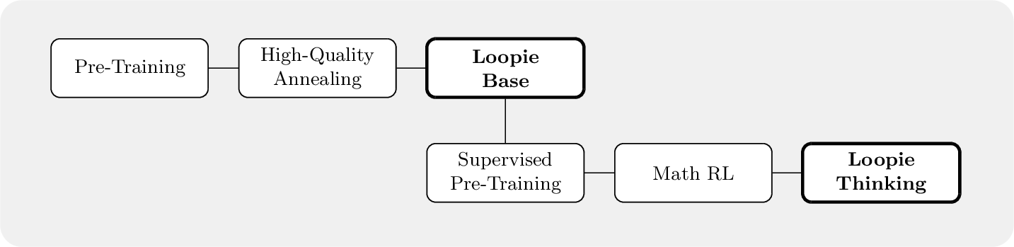
Loopie’s post-training recipe consists of two main stages following Stage 2 high-quality annealing. First, we introduce a supervised pre-training stage in which we continue training the model on 2T tokens of instruction-following, reasoning, coding, mathematics, and tool-use data, allowing the base model to acquire broad task-following and problem-solving capabilities while preserving the knowledge and general capabilities learned during pre-training. Second, we apply large-scale reinforcement learning to further enhance Loopie’s reasoning capabilities, improve its long-horizon problem solving, and align the model so that it produces reliable thinking traces. Together, these stages transform Loopie Base into the final Loopie Thinking model.
4.1 Supervised Pre-Training↩︎
We introduce supervised pre-training (SPT), a training regime that combines the supervision pattern of supervised fine-tuning (SFT) with the optimization scale of language-model pre-training (PT). SPT uses exactly the same training data and token-level objective as SFT: prompt and context tokens are excluded from the loss, and only supervised target tokens contribute to optimization. Unlike conventional SFT, however, SPT uses global batch sizes, sequence lengths, and token budgets typical of language-model pre-training.
| SPT | SFT | PT | |
|---|---|---|---|
| Loss function | Cross-entropy | Cross-entropy | Cross-entropy |
| Loss-bearing positions | Supervised target tokens only | Supervised target tokens only | All non-padding tokens |
| Pre-training metrics | \(\uparrow\) | \(\downarrow\) | \(\uparrow\) |
| Reasoning metrics | \(\uparrow\) | \(\uparrow\) | \(\approx\) |
| Overfitting after multiple epochs | Not observed | Observed | Not observed |
| Global batch size | \(\geq 1{,}024\) | \(32\)–\(128\) | \(\geq 1{,}024\) |
| Sequence length | \(\geq 128\,\mathrm{K}\) | \(8\)–\(32\,\mathrm{K}\) | \(4\)–\(8\,\mathrm{K}\) |
| Nominal token positions per batch | \(\geq 128\,\mathrm{M}\) | \(128\,\mathrm{K}\)–\(1\,\mathrm{M}\) | \(8\)–\(32\,\mathrm{M}\) |
| Total training token budget | \(\geq 2\,\mathrm{T}\) | \(10\)–\(100\,\mathrm{B}\) | \(\geq 4\,\mathrm{T}\) |
5pt
SPT separates two design choices that are commonly coupled: (i) which tokens contribute to the training loss, and (ii) the scale at which optimization is performed. SFT and SPT share the former choice, whereas PT and SPT share the latter. Consequently, SPT does not interpolate between an SFT loss and a PT loss. Instead, it applies an SFT-style supervised objective in a PT-scale optimization regime.
4.1.0.1 Training objective.
Consider a supervised example \(z_i = [c_i; y_i]\), where \(c_i\) denotes the input context and \(y_i\) denotes the supervised target response. Let \(w_{i,t} \in \{0,1\}\) be a binary loss mask for the token at position \(t\). All three training regimes use token-level cross-entropy: \[\mathcal{L}_{\mathrm{CE}}(\theta; w) = - \frac{ \displaystyle \sum_{i=1}^{B} \sum_{t=1}^{T_i} w_{i,t} \log p_{\theta} \left( z_{i,t} \mid z_{i,<t} \right) }{ \displaystyle \sum_{i=1}^{B} \sum_{t=1}^{T_i} w_{i,t} }. \label{eq:spt-loss}\tag{1}\] For both SPT and SFT, \(w_{i,t}=1\) only when \(z_{i,t}\) belongs to the supervised target \(y_i\); prompt, context, and padding positions are masked out. In conventional PT, by contrast, \(w_{i,t}=1\) for every non-padding token. Thus, all three regimes employ the same cross-entropy loss, but differ in the positions to which the loss is applied and in the scale of optimization.
Table 2 summarizes these distinctions. For representative SFT settings, including global batch sizes, training token counts, and sequence lengths, we primarily follow the configurations reported for OLMo 3, the Nemotron 3 series, and Step-3.5-Flash [59]–[64]. We use pre-training metrics to refer to metrics that evaluate general base-model capabilities and reasoning metrics to refer to metrics that primarily evaluate performance on challenging reasoning tasks, such as competition-level mathematics and coding problems. In our experiments, SPT improves performance on both types of metrics simultaneously. In contrast, the conventional SFT baseline only improves performance on reasoning metrics but degrades performance on pre-training metrics, whereas PT improves pre-training metrics performance while leaving performance on reasoning metrics approximately unchanged.
4.1.0.2 Pre-training-scale optimization over supervised data.
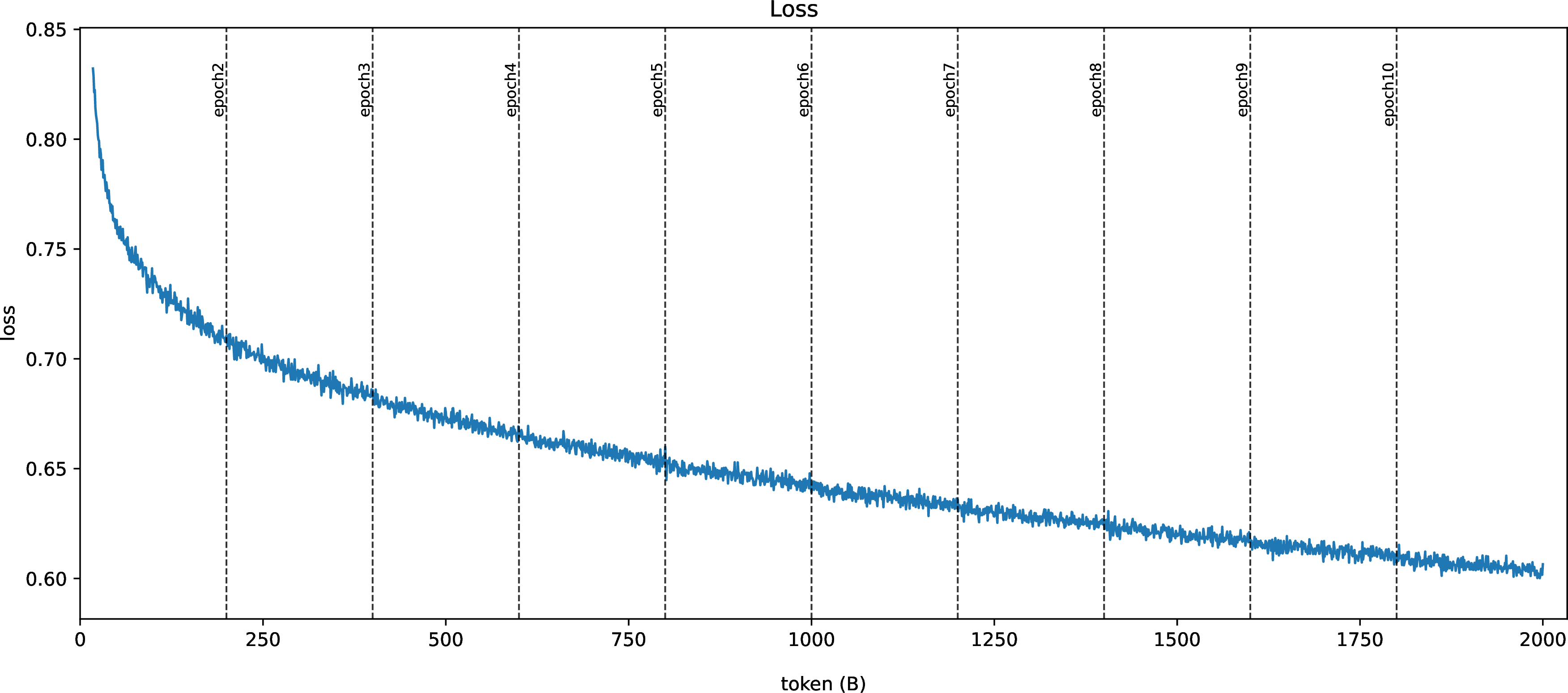
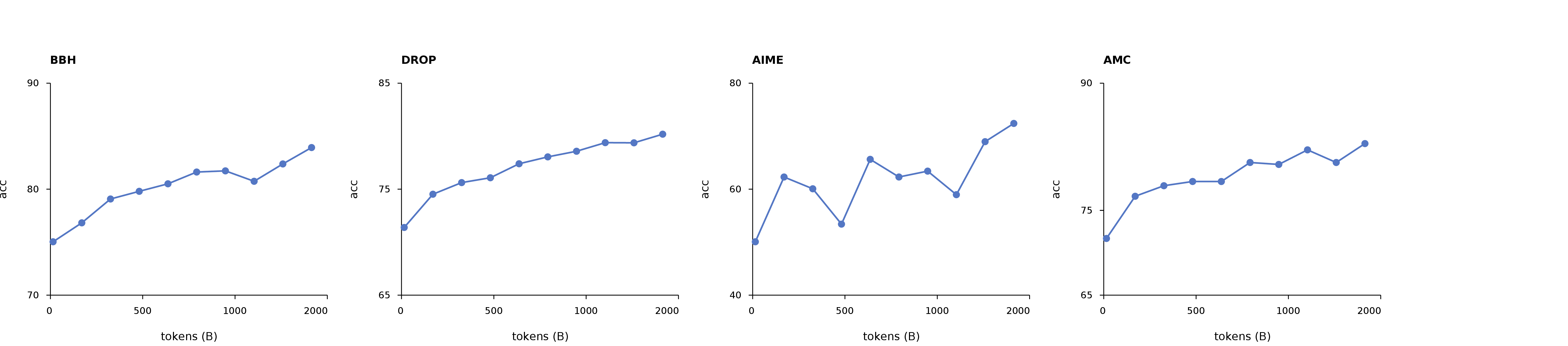
SPT processes 128 million tokens per global batch, approximately 1,000 times the number processed per batch in conventional SFT. This makes overfitting much less likely in SPT than in standard SFT. This scale gives SPT distinct training dynamics, consistent with observations that optimization hyperparameters and scaling behavior can change in large-language-model training regimes [65]. Under SPT, the model can be trained smoothly for substantially more epochs without showing signs of overfitting, such as abrupt drops in loss at epoch boundaries. At the same time, performance on downstream metrics continues to improve steadily. In addition, SPT mitigates catastrophic forgetting [66], which is a major drawback of conventional SFT and typically causes substantial degradation of the general knowledge acquired during pre-training. Notably, SPT not only avoids this degradation but also further improves general-knowledge performance.
As shown in Figure 11, SPT consistently improves performance on downstream pre-training metrics, including ARC-Challenge and MMLU, throughout approximately 10 epochs of training on 2T tokens. This finding challenges the conventional view that SFT leads to catastrophic forgetting.
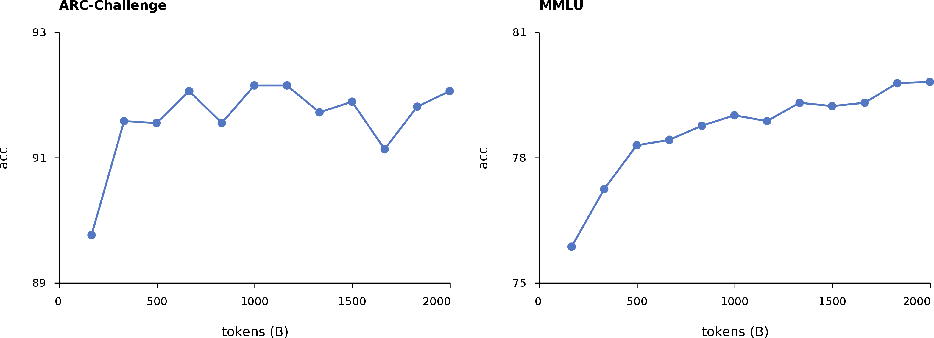
Simply running a conventional SFT configuration for more epochs does not reproduce the optimization regime of SPT. Conventional-scale SFT often begins to overfit between the second and fourth epochs. In small-batch SFT, each epoch involves many parameter updates computed from small batches, and repeated exposure to the same examples can lead to rapid specialization and memorization. In contrast, every SPT update aggregates supervision from more than one thousand sequences and over one hundred million nominal token positions. We hypothesize that this broad gradient aggregation, together with long contexts and a large token budget, mitigates the overly narrow specialization commonly observed during repeated SFT.
4.2 Reinforcement Learning↩︎
After SPT, we apply a reinforcement-learning stage to obtain Loopie Thinking. Following prior work, we do not mix data from multiple domains during training because domain-specific length biases may interfere with one another [67], [68]. We first conduct reinforcement learning on mathematical tasks; once performance saturates, we continue with reinforcement learning on coding tasks.
4.2.0.1 Algorithm.
Our optimizer builds on Group Sequence Policy Optimization (GSPO) [69], with the asymmetric clipping and dynamic sampling techniques introduced by DAPO [70]. For each prompt \(q\), we sample a group of \(G\) completions \(\{o_i\}_{i=1}^{G}\) from the old policy \(\pi_{\theta_{\mathrm{old}}}\) and score each completion using a verifier, yielding outcome rewards \(\{R_i\}_{i=1}^{G}\). We estimate sequence-level advantages by normalizing rewards within the sampled group: \[\hat{A}_i = \frac{ R_i - \operatorname{mean}(\{R_j\}_{j=1}^{G}) }{ \operatorname{std}(\{R_j\}_{j=1}^{G}) + \epsilon }, \label{eq:rl-group-advantage}\tag{2}\] where \(\epsilon\) is a small numerical constant.
Unlike token-level policy optimization, GSPO defines a length-normalized sequence-level importance ratio: \[s_i(\theta) = \left( \frac{\pi_{\theta}(o_i \mid q)}{\pi_{\theta_{\mathrm{old}}}(o_i \mid q)} \right)^{\frac{1}{|o_i|}} = \exp \left( \frac{1}{|o_i|} \sum_{t=1}^{|o_i|} \log \frac{\pi_{\theta}(o_{i,t} \mid q, o_{i,<t})}{\pi_{\theta_{\mathrm{old}}}(o_{i,t} \mid q, o_{i,<t})} \right).\] That is, \(s_i(\theta)\) is the geometric mean of the token-level importance ratios over the response. The length normalization reduces the variance of the sequence-level ratio and keeps responses of different lengths within a comparable numerical range.
The policy is optimized using a sequence-level clipped objective: \[\mathcal{J}_{\mathrm{RL}}^{\mathrm{GSPO}}(\theta) = \mathbb{E}_{ q \sim \mathcal{D},\, \{o_i\}_{i=1}^{G} \sim \pi_{\theta_{\mathrm{old}}}(\cdot \mid q) } \left[ \frac{1}{G} \sum_{i=1}^{G} \min \left( s_i(\theta)\hat{A}_i,\, \operatorname{clip} \left( s_i(\theta), 1-\epsilon_{\mathrm{low}}, 1+\epsilon_{\mathrm{high}} \right) \hat{A}_i \right) \right]. \label{eq:gspo-objective}\tag{3}\] In contrast to token-level clipping, GSPO applies the clipping operation to the entire response. Consequently, all tokens in the same response share the same sequence-level importance weight, aligning the unit of off-policy correction and optimization with the unit of reward.
Following the Clip-Higher strategy, we use \(\epsilon_{\mathrm{high}} > \epsilon_{\mathrm{low}}\). Under GSPO, this asymmetric clipping is applied to the sequence-level importance ratio rather than individual token-level ratios. The larger upper clipping range allows positively advantaged exploratory responses to receive stronger probability-increasing updates, while the more conservative lower clipping range limits excessive probability decreases for negatively advantaged responses.
We further apply prompt-level dynamic filtering. A prompt is retained only when its sampled group contains both successful and unsuccessful completions: \[0 < \sum_{i=1}^{G} \mathbf{1}\{R_i = R_{\mathrm{pass}}\} < G. \label{eq:dynamic-filtering}\tag{4}\] Groups that are entirely correct or entirely incorrect provide no useful relative preference signal for GRPO. We therefore oversample candidate prompts and filter out such groups until the effective batch is full. This keeps the optimization focused on prompts that yield non-degenerate policy gradients.
4.2.0.2 Training data.
We use the mathematics and code subsets of the Guru-RL corpus [71]. The mathematics pool is drawn from the OR1, DAPO, and DeepScaleR sources [70], [72], [73]. The code pool combines LeetCodeDataset, TACO-Verified, PrimeIntellect/SYNTHETIC-1, and historical LiveCodeBench training problems [74]–[78]. We apply an additional curation pass that removes malformed prompts, unverifiable answers, flaky tests, duplicate examples, and examples that substantially overlap with held-out evaluation sets. Rewards for mathematical problems are computed using rule-based answer equivalence, whereas rewards for coding problems are computed using sandboxed unit-test execution.
4.2.0.3 Training schedule.
We train in two context-length stages. The first stage uses a maximum response length of \(32\)K tokens. This stage is computationally efficient because most rollouts terminate naturally within this limit. When the rollout truncation rate exceeds \(10\%\), we switch to a \(64\)K-token stage, giving the policy additional room for longer derivations and code-reasoning trajectories. We continue RL until the aggregate validation score stops improving and begins to decline; the checkpoint immediately before sustained degradation is selected as Loopie Thinking. Throughout training, we monitor validation accuracy, mean response length, generation entropy, and truncation rate to detect late-stage over-optimization.
4.3 Results↩︎
We report two complementary comparisons of the final Loopie Thinking models. We compare Loopie-20B-A2B with MoE reasoning models at a similar active-parameter scale, and Loopie-6B-A0.6B with a broader set of compact reasoning models. All evaluations in
this section are conducted using the EvalScope framework, and the IFEval score is reported under the inst_level_loose setting. For AIME 2024 and AIME 2025, we report avg\(@\)8 results; for all other benchmarks,
we report pass\(@\)1. The AIME result shown in the teaser figure is for AIME 2024.
0.1pt
max width=
Table ¿tbl:tab:model-comparison? highlights the pre-training efficiency of Loopie-20B-A2B. Loopie is pre-trained on only 3.5T tokens, whereas Nemotron 3 Nano and Nemotron Cascade 2 are each trained on 25T tokens drawn from the same pre-training data source. Thus, Loopie uses less than one seventh of their pre-training tokens, yet matches or outperforms both models on most knowledge and general-capability benchmarks. In particular, Loopie reaches 81.28 on MMLU, exceeding both Nemotron 3 Nano (80.52) and Nemotron Cascade 2 (81.22). On ARC-Challenge, Loopie scores 93.52, outperforming Nemotron 3 Nano by 1.56 points and coming within 0.34 points of Nemotron Cascade 2. It also substantially surpasses both models on BBH, with a score of 82.28 versus 68.76 and 75.86, and on IFEval, with 84.72 versus 77.05 and 79.21.
This advantage extends across the broader pre-training evaluation suite: Loopie exceeds at least one of the two Nemotron models on every reported knowledge or general-capability benchmark and outperforms each of them on five of the seven benchmarks, despite having a pre-training token budget more than seven times smaller. The resulting profile is therefore not merely competitive at a smaller training budget; it indicates substantially higher token efficiency under the same pre-training data. Loopie also retains strong post-training reasoning performance, reaching 92.09 on AIME 2024 and 94.21 on AMC, ranking second among the listed models on both benchmarks, while its AIME 2025 score of 83.75 ties Qwen3-30B-A3B Thinking.
0.1pt max width=
5 International Mathematical Olympiad (IMO)↩︎
We follow the generate–verify–refine test-time scaling pipeline of prior work [79] and allocate a large inference-time compute budget to evaluate Loopie-20B-A2B on the 2025 IMO problems. For each problem, we initialize a candidate pool with 64 independently generated solutions and sample 64 verification analyses for each candidate. We rank the candidates according to their average verification scores and retain the top 64 solutions. For each retained solution, we sample eight verification analyses, prioritizing critiques that identify concrete errors, logical gaps, or missing justifications, and use the resulting solution–critique pairs to generate refined solutions. The refined solutions are added back to the candidate pool. This procedure is repeated for up to 16 iterations, with early termination when a candidate passes all 64 verification attempts. Finally, we select the solution with the highest aggregated verification score for evaluation, Each question was scored by GPT-5.5 acting as an LLM-as-a-judge. The evaluation was repeated three times, and the average score was reported. Further details are provided in Appendix E.
| IMO 2025 | |||||||
|---|---|---|---|---|---|---|---|
| Loopie-20B-A2B w/ TTS | \(7\) | \(7\) | \(4\) | \(6\) | \(7\) | \(4\) | \(35\) |
5.8pt
6 International Physics Olympiad (IPhO)↩︎
Following the generate–verify–refine pipeline used for IMO, we apply a similar generate–vote–critic test-time scaling strategy to the IPhO problems. Our procedure largely follows prior work [80], while allocating additional refinement rounds to accommodate the longer reasoning chains and more involved calculations required in physics problems. With extensive test-time scaling, Loopie-20B-A2B achieved a gold-medal-level score of 20.3 on the IPhO, surpassing the gold medal threshold of 19.7 points.
7 Related Work↩︎
7.1 Looped Transformers↩︎
We use the term looped model to denote an architecture that reuses a learned internal operator within a single forward computation, rather than repeatedly calling an otherwise complete model. This design lineage predates contemporary language models: Neural GPUs repeatedly apply a shared convolutional transition to learn algorithms, Adaptive Computation Time (ACT) learns how many recurrent updates to execute, Universal Transformers (UTs) tie self-attention and transition blocks across depth, and Deep Equilibrium Models (DEQs) avoid explicit unrolling by solving for a fixed point of a weight-tied transformation [1], [81]–[84]. Work on training implicit models and on generalist neural algorithmic learners further established practical optimization methods and reusable processors for effectively unbounded or task-shared computation. These are direct architectural antecedents of looped Transformers, not merely generic recurrent or test-time-compute methods.
Across Transformer families, layer tying, recurrent state, adaptive depth, and memory reuse also appear in ALBERT, tied Transformers, depth-adaptive Transformers, feedback memory, recurrent-memory Transformers, and block-recurrent Transformers [2], [85]–[89]. Modern variants make the shared-depth computation itself the central scaling axis. MoEUT recurrently reuses fine-grained expert groups, Relaxed Recursive Transformers supplement a repeated block with depth-specific low-rank adapters, and implicit state-space language models iterate a shared transition toward a fixed point while preserving substantial training parallelism [34]. Thus, rather than relying on ordinary depth scaling, looped Transformers learn a reusable transition \(h_{t+1}=F_{\theta}(h_t,x,e_t)\), where \(e_t\) may encode the loop index, a halting state, or an injected copy of the input. Effective inference depth can then vary without introducing an independently parameterized layer at every step.
7.2 Inductive Biases↩︎
Looped depth imposes several biases that are weak or absent in a stack of independent Transformer layers. First, recurrent operator sharing encourages a reusable update rule rather than a sequence of layer-specific feature maps. This is the defining recursive bias of UTs and tied-depth models, and theoretical analyses connect it to fixed-point iteration, gradient-based in-context learning, normalized gradient descent, and power iteration [1], [4], [15], [17], [36], [90]. Second, shared depth decouples effective computation from parameter count: a compact recurrent core can be unrolled for more steps, favoring iterative refinement over memorizing a separate computation in each layer [2], [7], [9], [10], [91].
Third, looping induces an iterative-algorithm bias. When a target computation is naturally expressed by repeated application of a small rule set, looped models can emulate programs, optimization procedures, graph algorithms, and structured algorithmic processors, often improving length or depth extrapolation when the loop count adapts to problem size [13], [14], [92]–[94]. Fourth, weight sharing creates a knowledge re-access and compositionality bias: after each new bridge entity is inferred, the same retrieval, binding, and update machinery can be applied again. This directly targets failures of implicit multi-hop composition in ordinary Transformers and motivates architectures that carry discrete and continuous states or align latent and explicit reasoning [95]–[101]. Fifth, recurrence provides a latent scratchpad and an adaptive-computation bias. Additional computation occurs in the hidden state rather than through the generation of extra verbal tokens, while timestep conditioning, token-wise routing, dynamic halting, fixed-point convergence, and shortcut consistency allocate more computation to harder inputs [7]–[9], [18], [102], [103]. These benefits are not automatic: looped models can drift, overthink, or collapse to shallow computation unless their state injection, normalization, supervision, and stopping rules are designed for stable iteration [104]–[107].
7.3 Theory, Mechanisms, and Scaling↩︎
Formal results characterize both the capabilities and the limits of shared-depth computation. Looped Transformers can execute instruction-level programs, simulate latent chains of thought, and achieve better approximation rates through timestep modulation [7], [14], [108]. More specialized analyses show that a recurrently reused attention layer can learn normalized-gradient updates for in-context logistic regression or implement the power method under layer normalization [90]. At the same time, compressed recurrent states create a memory-budget separation relative to full sequence-state chain-of-thought methods, and set-valued or graph computations require careful distinctions among fixed points, convergence, and halting. A complementary reinforcement-learning analysis formalizes how additional internal computation changes the class of compute-bounded policies.
A second line of work studies optimization, stability, and scaling with loop count. Fixed-point analyses identify conditions under which recurrent states remain reachable, input-dependent, and trainable; residual-scaling theory argues that correlated tied-block updates require loop-aware scaling; and iso-depth studies quantify the exchange rate among recurrent passes, unique depth, and training compute [91], [105], [109]. Two-scale latent-dynamics analyses derive convergence-sensitive early-exit criteria, while controlled studies of adaptive computation show that learned loop allocation can correlate with token difficulty without necessarily extrapolating to longer inputs [107], [110]. Memory tokens and ACT initialization can determine whether a UT enters a non-trivial reasoning regime, and hierarchical and flat recurrence can exhibit materially different optimization behavior even under shared-weight controls [111], [112]. Compression studies likewise show that preserving per-cell accuracy or local states is insufficient if quantization or pruning damages the recursive trajectory needed for exact solutions.
Mechanistic work examines what is represented across recurrent steps. Probing studies find that recurrent language models often approach loop-specific fixed points or replay feed-forward-like inference stages, while evidence for a literal latent chain-of-thought is mixed and depth-dependent [113], [114]. Shared recurrent modules can nevertheless specialize to perform distinct functional roles through asymmetric state identities, and interaction-locality measurements reveal how repeated local updates accumulate into global puzzle structure. Other probes recover relational preference information from differences between loop states, and analyses of tabular foundation models use the observed layer redundancy to motivate a single repeatedly applied layer. Finally, recurrent-depth models can unlock systematic multi-hop generalization, but autoregressive controls show that the benefit depends on where compute is placed rather than on recursion alone [99], [106].
7.4 Architectures, Training Objectives, and Inference↩︎
Recent looped language models treat recurrence as a third scaling axis alongside parameter count and token count. Huginn and Ouro pretrain recurrent-depth language models whose shared cores can be unrolled for variable test-time depth, while retrofitted recurrence and LoopUS convert pretrained feed-forward models into latent-refinement systems without training a recurrent model entirely from scratch [9], [10], [115], [116]. HRM-Text and CHERRY explore recurrent compression of deep language models, Hyperloop repeats only a middle block with cross-loop connections, and LoopMoE, sparse looped layers, and universal expert pools combine iterative depth with conditional capacity [117]–[121]. MoEUT and Relaxed Recursive Transformers provide earlier expert-routing and low-rank mechanisms for recovering expressivity under parameter sharing [34].
Dynamic-depth architectures decide not only how to update a state but also where and for how long to recur. Mixture-of-Recursions routes tokens to different depths; CoTFormer exposes earlier recurrent representations and learns a compute-budgeted router; AdaPonderLM and Think-at-Hard allocate extra latent iterations selectively; and Chain-of-Layers methods skip or repeat pretrained layers at test time [8], [102], [122], [123]. LoopFormer regularizes trajectories across sampled depths, adaptive-loop models couple halting with external memory, and ChainGPT, MoDr, and depth-recurrent attention mixtures enrich the recurrent state transition through multi-rank updates, branch routing, or mixtures of sequence and depth attention [11], [18], [124], [125]. SpiralFormer instead changes the resolution schedule across repeated applications, and subgoal-persistence models study when a hierarchical reasoner should re-plan rather than update the same latent plan at every step [126], [127].
A parallel line of work targets stable and efficient unrolling. Parallel Loop Transformers share representations across loops, and LT2 replaces quadratic attention with a linear-time looped design [128], [129]. MELT keeps cache memory independent of loop depth; LASER compresses recursive activations during training; and Hyperloop and CHERRY reduce the number of distinct parameter blocks [118], [119], [130]. Parcae constrains recurrent dynamics and derives scaling laws, CART anchors each iteration to context, fully looped signal routing stabilizes high loop counts, stochastic stopping improves extrapolation across unseen depths, and stability-aware recurrent training reduces drift under test-time scaling [19], [131]–[133]. Training-free looping explores whether a pretrained model can be recurrently reused without architectural retraining [134].
Several methods supervise the trajectory rather than the final answer alone. LoopRPT applies reinforcement pre-training across latent iterations, RLTT distributes reward over the latent trajectory, denoising recursion trains models to repeatedly correct corrupted targets, and Generative Recursive Reasoning expands recurrence into stochastic multi-trajectory generation [135]–[137]. Probabilistic TRM injects noise at inference and selects among recursive trajectories, whereas LoopFormer uses shortcut consistency to align different computation budgets [18], [138]. Looped diffusion language models, fixed-point masked generative models, equilibrium reasoners, and attractor models connect explicit recurrence to denoising or convergence-based generation [139], [140]. These approaches make intermediate-state quality, convergence geometry, and trajectory diversity first-class training targets rather than incidental by-products of depth.
7.5 In-Context, Algorithmic, and Compositional Generalization↩︎
In-context learning can be interpreted as executing an implicit learning algorithm over demonstrations. Bayesian, gradient-descent, preconditioned-gradient, linear-model, and causal-structure accounts motivate studying whether each recurrent step implements one additional internal update [141]–[147]. Looped Transformers make this correspondence explicit: they learn data-fitting algorithms with substantially fewer unique parameters, implement multi-step gradient procedures, and can use distinct preprocessing, looping, and postprocessing stages [4], [15], [17], [93]. Program-simulation results and normalized-gradient analyses further connect shared depth to reusable algorithmic primitives [14].
The same prior is relevant to length and compositional extrapolation. Neural GPUs and generalist recurrent processors learn repeated algorithmic updates, while looped Transformers simulate graph algorithms and obtain strong length generalization when the number of recurrent steps grows with the instance [13], [81], [92]. Timestep modulation, multi-resolution recursion, and depth-recurrent compositional models address the failure of a single stationary update to remain useful far beyond the trained depth [108], [126], [148]. DiscoLoop carries both discrete embeddings and continuous hidden states across hops, and LOTUS aligns recurrent latent blocks with explicit chain-of-thought computation [100], [101]. These results complement evidence that ordinary Transformers often memorize local facts or short computations yet fail to compose them systematically out of distribution [96], [98], [149].
7.6 Abstract Reasoning↩︎
ARC-style tasks are a natural stress test because they require inducing a new transformation from a few demonstrations rather than recalling a fixed skill [150], [151]. HRM obtains substantial effective depth through coupled high- and low-level recurrent modules, TRM reduces the design to a tiny repeatedly applied network, and the URM study attributes much of the gain to Universal-Transformer-style recurrence and nonlinear depth computation [3], [5], [6]. Controlled analyses caution that hierarchy, augmentation, identity conditioning, majority voting, and competition-time adaptation can materially affect reported scores [152]–[155].
Follow-up designs explore complementary ways to improve recursive abstract reasoning. CosmicFish-HRM adapts hierarchical recurrence to compact language models; Recursive Inference Machines generalize generator–solver recursion; and Fixed-Point Reasoners halt upon convergence rather than at a preset depth [103], [156], [157]. Generative, probabilistic, and denoising recursive models introduce trajectory diversity or iterative corruption-and-repair curricula [136]–[138]. Equilibrium and attractor reasoners learn convergent solution dynamics, whereas Tiny Autoregressive Recursive Models test whether comparable compute is better spent on recurrence or ordinary autoregressive depth [106], [140]. Memory-augmented UTs, LoopViT, and interaction-locality analyses expose complementary depth–state, visual-recurrence, and mechanism-level views [111], [158]. Overall, this literature supports recurrence as an architectural prior for iterative abstraction, while showing that successful test-time scaling depends on stable state transitions and informative intermediate supervision rather than loop count alone [159], [160].
8 Future Work↩︎
Due to computational constraints, our post-training experiments focus primarily on mathematical and code reasoning tasks. We do not extensively explore other important capabilities studied in prior work, such as scientific question answering, instruction following, alignment with human conversational preferences, or agentic task-solving. A natural direction for future work is to continue to post-train Loopie on a broader set of tasks and preference signals, which may further improve its practical utility and general-purpose capabilities. Also, due to limited computational resources, we were unable to conduct a sufficiently comprehensive ablation study of supervised pre-training, which we leave for future work.
In addition, our study focuses primarily on matching compute budgets during pre-training, and we have not yet conducted systematic studies of inference-time computation. Matching and optimizing inference-time compute remain important directions for future work; prior work such as the Parallel Loop Transformer [128] provides a promising example of this approach.
Finally, our study intentionally focuses on applying looped Transformers to a relatively clean and well-controlled base architecture, Qwen3-30B-A3B, in order to avoid confounding factors introduced by architectural variations. As a result, we do not investigate several recent architectural advances that may be complementary to our method. Exploring how Loopie interacts with these newer designs remains an important direction for future work.
9 Conclusion↩︎
We introduced Loopie, a family of looped MoE language models that makes recurrent depth competitive under a matched pre-training compute budget. By combining layer-loop recurrence with a hardware-aware scaling recipe, Loopie consistently outperforms compute-matched vanilla Transformer baselines across model scales. A large-scale post-training pipeline based on Supervised Pre-training and reinforcement learning further equips Loopie with strong mathematical reasoning and coding abilities. These results suggest that recurrent computation, when jointly optimized with architecture and training efficiency, can serve as a practical scaling axis for large language models.
Author Contributions↩︎
Zitian Gao completed model training, experimental implementation, and writing of this paper. The model architecture was designed by Zitian Gao, Yilong Chen, Yihao Xiao, and Xinyu Yang, with guidance from Ran Tao, Joey Zhou, and Bryan Dai. Yilong Chen and Xinyu Yang completed this work during their internship at IQuest Research.
10 Acknowledgments↩︎
We thank Benhao Huang at Carnegie Mellon University and Shaowen Wang at Tsinghua University for their valuable feedback and careful review.
We thank Zhengmao Ye at IQuest Research for his infrastructure support.
We thank NVIDIA Nemotron for its outstanding contributions to the open-source community. In particular, Loopies would not have achieved its current level of performance without the training data provided by Nemotron-CC-v2 and Nemotron-Cascade-2.
We thank the Allen Institute for AI (AI2) for the elegant LaTeX template used in this work.
Architecture Details↩︎
Pre-training Details↩︎
Scaling Ladder Details↩︎
| Rung | Model | ||||||||||
| Params | |||||||||||
| Params | \(L\) | \(D\) | \(D_{\mathrm{MoE}}\) | Heads | |||||||
| Dim | \(N\) | ||||||||||
| Depth | Tokens | ||||||||||
| 1 | Vanilla | 1.34B | 0.15B | 27 | 640 | 192 | 20 | 32 | 1 | 23.70 | 150B |
| Loopie | 1.08B | 0.11B | 15 | 704 | 256 | 22 | 32 | 2 | 23.47 | 150B | |
| 2 | Vanilla | 2.37B | 0.25B | 30 | 768 | 256 | 24 | 32 | 1 | 25.60 | 250B |
| Loopie | 1.81B | 0.18B | 17 | 832 | 320 | 26 | 32 | 2 | 24.47 | 250B | |
| 3 | Vanilla | 4.76B | 0.51B | 36 | 1280 | 320 | 32 | 40 | 1 | 35.56 | 500B |
| Loopie | 3.78B | 0.41B | 19 | 1280 | 384 | 32 | 40 | 2 | 33.68 | 500B | |
| 4 | Vanilla | 9.14B | 1.00B | 46 | 1280 | 384 | 40 | 32 | 1 | 27.83 | 500B |
| Loopie | 6.36B | 0.68B | 25 | 1408 | 448 | 44 | 32 | 2 | 28.16 | 500B |
Supervised Pre-training Details↩︎
Model Solutions for IMO 2025↩︎
The model’s original response was provided in Markdown format, which cannot be rendered directly in LaTeXin this context. We therefore used GPT-5.5 to convert the Markdown content into LaTeX and manually verified that the converted version was consistent with the model’s original response. The judgments produced by the GPT-5.5-based evaluator may contain errors. If you identify any incorrect scores among those reported below, we would appreciate it if you could contact us promptly.
A line in the plane is called sunny if it is not parallel to any of the \(x\)-axis, the \(y\)-axis, or the line \(x+y=0\).
Let \(n \ge 3\) be a given integer. Determine all nonnegative integers \(k\) such that there exist \(n\) distinct lines in the plane satisfying both of the following:
for all positive integers \(a\) and \(b\) with \(a+b\le n+1\), the point \((a,b)\) lies on at least one of the lines; and
exactly \(k\) of the \(n\) lines are sunny.
Solution
Judge
Reported score: \(7/7\). Judge model: gpt-5.5. Response score tags: \(7/7,\;7/7,\;7/7\).
For an integer \(n\ge 3\) define \[P_n = \{(a,b)\in\mathbb{N}^2 \mid a\ge 1,\; b\ge 1,\; a+b\le n+1\}.\] The points of \(P_n\) are exactly the lattice
points in the triangle with vertices \((1,1)\), \((1,n)\), \((n,1)\).
A line is called sunny if it is not parallel to the \(x\)-axis, the \(y\)-axis, or the line \(x+y=0\); equivalently, its slope is
different from \(0\), \(\infty\), and \(-1\).
We must determine all non-negative integers \(k\) for which there exist \(n\) distinct lines satisfying
every point of \(P_n\) lies on at least one of the lines, and
exactly \(k\) of the lines are sunny.
1. Constructions for \(k=0,1,3\)↩︎
\(k=0\).
Take the vertical lines \(x=1,x=2,\dots,x=n\). They are distinct, each is parallel to the \(y\)-axis (hence not sunny), and every point \((a,b)\in P_n\) lies on \(x=a\). Thus we obtain a covering with \(0\) sunny lines.\(k=1\).
Take the vertical lines \(x=1,x=2,\dots,x=n-1\) (there are \(n-1\) of them) and one sunny line through \((n,1)\) with slope \(1\), for instance \(y = x - n + 1\).
The vertical lines cover all points with first coordinate \(\le n-1\); the only point with \(a=n\) is \((n,1)\) (because \(a+b\le n+1\) forces \(b=1\)). This point lies on the sunny line. Hence all points of \(P_n\) are covered, and exactly one line (the slanted one) is sunny.\(k=3\).
– For \(n=3\) we can use three sunny lines that cover \(P_3\), e.g. \[y = x,\qquad y = -\tfrac12 x + \tfrac52,\qquad y = -2x + 5.\] A direct check shows they cover the six points \((1,1),(1,2),(1,3),(2,1),(2,2),(3,1)\). All three have slopes \(1,-\frac{1}{2},-2\), none of which is \(0,\infty,-1\), so they are sunny.
– For \(n>3\) do the following:Add the \(n-3\) horizontal lines \(y=1, y=2, \dots, y=n-3\). (These are not sunny because they are parallel to the \(x\)-axis.)
Take the three sunny lines from the \(n=3\) construction and shift each of them upward by \(n-3\) (i.e., replace \(y = f(x)\) by \(y = f(x)+(n-3)\)).
After this shift, the three lines cover exactly the points of \(P_n\) with \(b\ge n-2\) (the map \((a,b)\mapsto (a,b-(n-3))\) sends that set bijectively onto \(P_3\)). Together with the horizontal lines, every point of \(P_n\) is covered. The three shifted lines remain sunny (slopes unchanged), and the \(n-3\) horizontal lines are not sunny. Hence we obtain exactly three sunny lines.
Thus for every \(n\ge 3\) the values \(k=0,1,3\) are attainable.
2. A lemma for \(n\ge 4\)↩︎
Consider the three sides of the triangle \(P_n\): \[L_x : x=1,\qquad L_y : y=1,\qquad L_d : x+y=n+1.\] Each side contains \(n\) points of \(P_n\) (the lattice points on that segment), but the three vertices \((1,1)\), \((1,n)\), \((n,1)\) belong to two sides each. Therefore the union \(L_x\cup L_y\cup L_d\) consists of \(3n-3\) distinct points of \(P_n\).
Lemma. For \(n\ge 4\), any family of \(n\) lines that covers \(P_n\) must contain at least one of the three lines \(L_x, L_y, L_d\).
Proof. Assume, to the contrary, that none of these three lines is among our \(n\) lines. Take any line \(\ell\) used in the covering. Since \(P_n\) is convex, its boundary is the union of the three sides. The intersection \(\ell\cap\partial P_n\) is a convex subset of the triangle, hence either empty, a single point (tangent at a vertex), or a line segment (with two endpoints). In all cases \(\ell\) contains at most two distinct boundary points. Consequently, each of our \(n\) lines can cover at most two of the \(3n-3\) boundary points. Together they can cover at most \(2n\) distinct boundary points. But \(2n < 3n-3\) for \(n\ge 4\), contradicting the fact that all boundary points must be covered. Hence at least one of the three sides must appear.
3. Induction↩︎
We prove by induction on \(n\) that if a covering of \(P_n\) by \(n\) distinct lines exists, then the number \(k\) of sunny lines among them satisfies \(k\in\{0,1,3\}\).
Base case \(n=3\).
Constructions for \(k=0,1,3\) are given in Section 1 (for \(k=1\) we use \(x=1,x=2\) and \(y=x-2\); for \(k=3\) the three sunny lines listed above). It remains to show that \(k=2\) is impossible.
Assume there is a covering of \(P_3\) with exactly two sunny lines and one non-sunny line. The non-sunny line must be horizontal, vertical, or have slope \(-1\). The points of \(P_3\) are \[A=(1,1),\; B=(1,2),\; C=(1,3),\; D=(2,1),\; E=(2,2),\; F=(3,1).\] A line with slope \(0,\infty,\) or \(-1\) can contain at most three of these points (e.g. \(x=1\) contains \(A,B,C\); \(y=1\) contains \(A,D,F\); \(x+y=4\) contains \(C,E,F\)). If it covers \(0\) or \(1\) point, then the two sunny lines would have to cover the remaining \(5\) or \(6\) points. But any sunny line can contain at most two points of \(P_3\) because the only triples of collinear points in \(P_3\) lie on the sides, which have forbidden slopes. Hence two sunny lines cover at most \(4\) distinct points, a contradiction. Thus the non-sunny line must cover either \(2\) or \(3\) points.
We now examine all non-sunny lines that contain at least two points of \(P_3\):
| Line | Points covered | Complement \(S\) |
|---|---|---|
| \(x=1\) | \(A,B,C\) | \(\{D,E,F\}\) |
| \(x=2\) | \(D,E\) | \(\{A,B,C,F\}\) |
| \(y=1\) | \(A,D,F\) | \(\{B,C,E\}\) |
| \(y=2\) | \(B,E\) | \(\{A,C,D,F\}\) |
| \(x+y=3\) | \(B,D\) | \(\{A,C,E,F\}\) |
| \(x+y=4\) | \(C,E,F\) | \(\{A,B,D\}\) |
For each \(S\) we check whether it can be covered by two sunny lines.
\(S = \{D,E,F\}\): every pair lies on a non-sunny line (\(D,E\) vertical, \(D,F\) horizontal, \(E,F\) slope \(-1\)). Hence no sunny line can contain two of these points; covering three points with two sunny lines would require at least one sunny line to contain two points – impossible.
\(S = \{A,B,C,F\}\): the only sunny pair is \((B,F)\) (slope \(-\frac{1}{2}\)). All other pairs are non-sunny. To cover four points we would need two sunny lines each covering two points, but only one sunny pair exists. Points \(A\) and \(C\) cannot be together on a sunny line (they determine \(x=1\), non-sunny) and would then need two separate sunny lines, making three sunny lines in total. Impossible.
\(S = \{B,C,E\}\): all pairs are non-sunny, so two sunny lines can cover at most two points.
\(S = \{A,C,D,F\}\): the only sunny pair is \((C,D)\) (slope \(-2\)). The remaining points \(A\) and \(F\) cannot be together on a sunny line (they determine \(y=1\), non-sunny) and would need two separate sunny lines. Impossible.
\(S = \{A,C,E,F\}\): the only sunny pair is \((A,E)\) (slope \(1\)). Points \(C\) and \(F\) cannot be together on a sunny line (slope \(-1\)), and would need two separate sunny lines. Impossible.
\(S = \{A,B,D\}\): no pair of points in \(S\) lies on a sunny line (\(A,B\) vertical, \(A,D\) horizontal, \(B,D\) slope \(-1\)). Thus two sunny lines cannot cover three points.
Hence no configuration with exactly one non-sunny line and two sunny lines can cover \(P_3\). Therefore \(k=2\) is impossible for \(n=3\), and the only possible values are \(k=0,1,3\).
Inductive step. Let \(n\ge 4\) and suppose a covering of \(P_n\) by \(n\) lines exists with exactly \(k\) sunny lines. By the lemma, at least one of the three sides \(L_x, L_y, L_d\) is among the lines. Remove that side; we are left with \(n-1\) lines. We show that these \(n-1\) lines (possibly after a translation) give a covering of \(P_{n-1}\) with the same \(k\).
We distinguish three cases.
Case 1 – the removed side is \(L_d : x+y=n+1\).
All points of \(P_n\) with \(a+b\le n\) (i.e., \(P_{n-1}\)) are not on \(L_d\), so they are covered by the remaining lines. Thus the remaining lines already cover \(P_{n-1}\). They are \(n-1\) distinct lines and keep their sunny status, giving a covering of \(P_{n-1}\) with \(n-1\) lines and \(k\) sunny lines.Case 2 – the removed side is \(L_x : x=1\).
The remaining lines cover all points with \(a\ge 2\) (points with \(a=1\) lie on \(L_x\) and are not covered by the others). Translate the whole plane left by one unit: \((x',y') = (x-1,y)\). Under this translation, the set \[\{(a-1,b) \mid a\ge 2,\; b\ge 1,\; a+b\le n+1\}\] becomes exactly \(P_{n-1}\). For each of the remaining \(n-1\) lines, apply the same translation to obtain a new line. A point \((a,b)\) with \(a\ge 2\) lies on a line \(L\) in the original configuration iff \((a-1,b)\) lies on the translated line. Hence the translated lines cover \(P_{n-1}\). Translation does not change slopes, so a sunny line remains sunny. The lines are still distinct. We have obtained a covering of \(P_{n-1}\) with \(n-1\) lines and \(k\) sunny lines.Case 3 – the removed side is \(L_y : y=1\).
Symmetric to Case 2: translate downward by one unit.
In each case we have reduced the problem from \(n\) to \(n-1\) while preserving \(k\). Since \(n-1\ge 3\), the induction hypothesis applies and forces \(k\in\{0,1,3\}\). This completes the induction for \(n\ge 4\).
4. Conclusion↩︎
For every \(n\ge 3\) we have shown:
There exist coverings with \(k=0,1,3\) sunny lines (explicit constructions).
Any covering must have \(k\in\{0,1,3\}\) (by induction, with base \(n=3\)).
Therefore the set of admissible integers \(k\) is exactly \(\boxed{\{0,1,3\}}\).
Judge Response 1
Score: \(7/7\).
Reason. The solution gives valid constructions for all claimed values k=0,1,3, proves the key boundary-line lemma correctly for n\(\ge\)4, handles the n=3 base case including impossibility of k=2, and uses a sound induction reducing by a non-sunny side while preserving the number of sunny lines. The argument is rigorous and complete.
Judge Response 2
Score: \(7/7\).
Reason. Complete and rigorous solution. The constructions for k=0,1,3 are valid, including the shifted k=3 construction. The boundary-counting lemma is correct for n>=4, and the induction preserves the number of sunny lines because the removed side is always non-sunny. The n=3 base case carefully rules out k=2. Only very minor wording imprecision occurs in referring to P_n as convex, but the intended convex hull argument is clear and valid.
Judge Response 3
Score: \(7/7\).
Reason. Complete and rigorous solution. It gives valid constructions for k=0,1,3, proves a correct boundary-line lemma for n\(\ge\)4, uses induction preserving the number of sunny lines, and handles the n=3 base case including impossibility of k=2 by exhaustive checking. Only minor wording imprecision appears in the induction, but it does not affect correctness.
Let \(\Omega\) and \(\Gamma\) be circles with centres \(M\) and \(N\), respectively, such that the radius of \(\Omega\) is less than the radius of \(\Gamma\). Suppose \(\Omega\) and \(\Gamma\) intersect at two distinct points \(A\) and \(B\). Line \(MN\) intersects \(\Omega\) at \(C\) and \(\Gamma\) at \(D\), so that \(C\), \(M\), \(N\), \(D\) lie on \(MN\) in that order. Let \(P\) be the circumcenter of triangle \(ACD\). Line \(AP\) meets \(\Omega\) again at \(E \neq A\) and meets \(\Gamma\) again at \(F \neq A\). Let \(H\) be the orthocenter of triangle \(PMN\).
Prove that the line through \(H\) parallel to \(AP\) is tangent to the circumcircle of triangle \(BEF\).
Solution
Judge
Reported score: \(7/7\). Judge model: gpt-5.5. Response score tags: \(7/7,\;7/7,\;7/7\).
We give a coordinate proof. By scaling we may assume \(MN = 1\).
Let the circles have centres
\[M=(0,0),\qquad N=(1,0),\]
radii \(r\) (circle \(\Omega\)) and \(R\) (circle \(\Gamma\)) with \(r<R\).
Since the circles intersect in two points we have \(|R-r|<1<R+r\).
Write
\[a = R-r>0,\qquad b = R+r>1.\]
Then
\[r = \frac{b-a}{2},\qquad R = \frac{b+a}{2},\qquad 0<a<1<b.\]
1. The points \(A\) and \(B\)↩︎
The equations are
\[\Omega:\; x^2+y^2=r^2,\qquad \Gamma:\; (x-1)^2+y^2=R^2.\]
Subtracting gives
\[-2x+1 = R^2-r^2 = ab \;\Longrightarrow\; x = \frac{1-ab}{2}=h.\]
Substituting into \(\Omega\) yields
\[t^2 = r^2-h^2 = \frac{(b^2-1)(1-a^2)}{4}>0,\]
hence
\[t = \frac{\sqrt{(b^2-1)(1-a^2)}}{2}>0.\]
Thus
\[A=(h,t),\qquad B=(h,-t).\]
2. The points \(C\) and \(D\)↩︎
On the line \(MN\) (the \(x\)-axis) we have the intersections
\[C = (-r,0) = \Bigl(-\frac{b-a}{2},0\Bigr), \qquad D = (1+R,0) = \Bigl(1+\frac{b+a}{2},0\Bigr)=\Bigl(\frac{b+a+2}{2},0\Bigr).\]
Because the order is \(C,M,N,D\) we have \(C<0<1<D\).
3. Circumcentre \(P\) of \(\triangle ACD\)↩︎
\(C\) and \(D\) lie on the \(x\)-axis, so the perpendicular bisector of \(CD\) is vertical.
The midpoint of \(CD\) has \(x\)-coordinate
\[\frac{x_C+x_D}{2}= \frac{-\frac{b-a}{2}+\frac{b+a+2}{2}}{2}= \frac{a+1}{2}.\]
Hence \(P\) has \(x\)-coordinate \(p = \dfrac{1+a}{2}\).
Let \(P=(p,y)\). Using \(PA=PC\) (equivalently \(PA=PD\) because \(P\) lies on the perpendicular bisector of \(CD\)) we obtain
\[(p-h)^2+(y-t)^2=(p-x_C)^2+y^2.\]
Insert \(p-h=\frac{a+b}{2}\), \(p-x_C=\frac{b+1}{2}\), \(t^2\) as above. After simplification
\[y = -\frac{(b^2-1)(1-a^2)}{4t}= -\frac{(b+1)\sqrt{1-a^2}}{2\sqrt{b^2-1}}.\]
Thus
\[P=\Bigl(\frac{1+a}{2},\; -\frac{(b+1)\sqrt{1-a^2}}{2\sqrt{b^2-1}}\Bigr).\]
4. Direction vector of \(AP\)↩︎
Set \(\vec{v} = \overrightarrow{AP}\). Then
\[\vec{v}_x = p-h = \frac{a+b}{2},\]
\[\vec{v}_y = y-t = -\frac{(b+1)\sqrt{1-a^2}}{2\sqrt{b^2-1}} - \frac{\sqrt{(b^2-1)(1-a^2)}}{2} = -\frac{b t}{b-1}.\]
So
\[\boxed{\;\vec{v} = \Bigl(\frac{a(1+b)}{2},\; -\frac{b t}{b-1}\Bigr)\; }.\]
5. The points \(E\) and \(F\)↩︎
Parametrise the line through \(A\) with direction \(\vec{v}\) as \(A+\lambda\vec{v}\).
For a circle with centre \(O\) and radius \(R\), the second intersection of this line with the circle is \(A+\lambda\vec{v}\) with
\[\lambda = -\frac{2\,(A-O)\cdot\vec{v}}{|\vec{v}|^2}.\]
We apply this to \(\Omega\) (\(O=M=(0,0)\)) and to \(\Gamma\) (\(O=N=(1,0)\)).
For \(\Omega\):
\[A\cdot\vec{v} = h\,\vec{v}_x + t\,\vec{v}_y = -\frac{(1+b)(b-a)}{4},\qquad |\vec{v}|^2 = \frac{(1+b)(b^2-a^2)}{4(b-1)}.\]
Hence
\[\lambda_E = -\frac{2(A\cdot\vec{v})}{|\vec{v}|^2} = \frac{2(b-1)}{b+a}.\]
For \(\Gamma\):
\[(A-N)\cdot\vec{v} = (h-1)\,\vec{v}_x + t\,\vec{v}_y = -\frac{(1+b)(a+b)}{4},\qquad |\vec{v}|^2 = \frac{(1+b)(b^2-a^2)}{4(b-1)}.\]
Thus
\[\lambda_F = -\frac{2((A-N)\cdot\vec{v})}{|\vec{v}|^2} = \frac{2(b-1)}{b-a}.\]
Consequently \(E = A+\lambda_E\vec{v}\) and \(F = A+\lambda_F\vec{v}\).
We shift coordinates by \((h,-t)\) so that \(B\) becomes the origin.
Define
\[X = x-h,\qquad Y = y+t.\]
For any point we write \(X',Y'\). Then
\[X' = \lambda\,\vec{v}_x,\qquad Y' = 2t + \lambda\,\vec{v}_y.\]
Using \(\lambda_E,\lambda_F\) we obtain
\[E' = \Bigl(\frac{a(b^2-1)}{b+a},\; \frac{2a t}{b+a}\Bigr),\qquad F' = \Bigl(\frac{a(b^2-1)}{b-a},\; -\frac{2a t}{b-a}\Bigr).\]
6. Circumcircle of \(\triangle BEF\)↩︎
Let the circle through \(B',E',F'\) have equation \(X^2+Y^2 + DX + KY = 0\) (centre \((-D/2,-K/2)\)).
Substituting \(E'\) and \(F'\) and solving for \(D,K\) gives
\[D = -a b,\qquad K = \frac{a^2(b^2-1)}{2 t}.\]
(Only one linear equation determines \(D\); the other then yields \(K\).)
Thus in the shifted coordinates the centre is \((a b/2,\; -K/2)\).
Transforming back to the original coordinates:
\[O = \Bigl(h+\frac{a b}{2},\; -t-\frac{K}{2}\Bigr).\]
Since \(h = \frac{1-ab}{2}\), we have \(h+\frac{a b}{2} = \frac{1}{2}\).
Using \(K = \frac{a^2(b^2-1)}{2 t}\) and \(4t^2 = (1-a^2)(b^2-1)\),
\[O_y = -t-\frac{a^2(b^2-1)}{4t} = -\frac{t}{1-a^2}.\]
Hence
\[\boxed{\;O = \Bigl(\frac{1}{2},\; -\frac{t}{1-a^2}\Bigr)\; }.\]
7. Orthocentre \(H\) of \(\triangle PMN\)↩︎
Vertices: \(M=(0,0)\), \(N=(1,0)\), \(P=\bigl(\frac{1+a}{2},\, y\bigr)\) with \(y\) as above.
The altitude from \(P\) is the vertical line \(x = \frac{1+a}{2}\).
The altitude from \(M\) is perpendicular to \(PN\). Since \(\overrightarrow{PN} = (p-1,\, y)\), its equation is
\[(p-1)x + y\,y = 0.\]
Intersecting with the altitude from \(P\) gives
\[y = -\frac{(p-1)p}{y}.\]
Using \(p-1 = \frac{a-1}{2}\) and \(y\) from above, after simplification
\[y = -\frac{t}{b+1}.\]
Thus
\[\boxed{\;H = \Bigl(\frac{1+a}{2},\; -\frac{t}{b+1}\Bigr)\; }.\]
8. Tangency of the line through \(H\) parallel to \(AP\)↩︎
The line through \(H\) parallel to \(AP\) is
\[\ell:\; (x,y) = H + \mu\vec{v},\qquad \mu\in\mathbb{R}.\]
We show that the distance from the centre \(O\) to \(\ell\) equals the radius of the circumcircle of \(\triangle BEF\).
The distance from a point \(O\) to a line through \(H\) with direction \(\vec{v}\) is
\[\operatorname{dist}(O,\ell) = \frac{\bigl|\,(\overrightarrow{HO}\times\vec{v})\,\bigr|}{|\vec{v}|}.\]
Compute
\[\vec{w} = O-H = \Bigl(-\frac{a}{2},\; O_y + \frac{t}{b+1}\Bigr) = \Bigl(-\frac{a}{2},\; t\Bigl(-\frac{1}{1-a^2} + \frac{1}{b+1}\Bigr)\Bigr).\]
Hence
\[O_y + \frac{t}{b+1} = t\cdot\frac{-b-a^2}{(1-a^2)(b+1)}.\]
Now
\[\vec{w} \times \vec{v} = w_x v_y - w_y v_x = \frac{a b t}{2(b-1)} + \frac{a t (b+a^2)}{2(1-a^2)}.\]
Simplifying the bracket:
\[\frac{b}{b-1} + \frac{b+a^2}{1-a^2} = \frac{b^2-a^2}{(b-1)(1-a^2)}.\]
Thus
\[\bigl|\,\vec{w} \times \vec{v}\,\bigr| = \frac{a t}{2}\cdot\frac{b^2-a^2}{(b-1)(1-a^2)}.\]
Using \(t = \frac{\sqrt{(b^2-1)(1-a^2)}}{2}\),
\[\bigl|\,\vec{w} \times \vec{v}\,\bigr| = \frac{a (b^2-a^2) \sqrt{b^2-1}}{4 (b-1) \sqrt{1-a^2}}.\]
Now
\[|\vec{v}| = \sqrt{\frac{(1+b)(b^2-a^2)}{4(b-1)}},\qquad R_B = \text{radius of }(BEF) = \frac{a \sqrt{b^2-a^2}}{2\sqrt{1-a^2}}.\]
Multiplying,
\[|\vec{v}|\,R_B = \frac{a (b^2-a^2) \sqrt{b+1}}{4 \sqrt{(b-1)(1-a^2)}}.\]
Since \(\sqrt{b^2-1} = \sqrt{(b-1)(b+1)}\),
\[\bigl|\,\vec{w} \times \vec{v}\,\bigr| = \frac{a (b^2-a^2) \sqrt{b^2-1}}{4 (b-1) \sqrt{1-a^2}} = \frac{a (b^2-a^2) \sqrt{b+1}}{4 \sqrt{(b-1)(1-a^2)}} = |\vec{v}|\,R_B.\]
Therefore
\[\operatorname{dist}(O,\ell) = \frac{\bigl|\,\vec{w} \times \vec{v}\,\bigr|}{|\vec{v}|} = R_B,\]
i.e. the line \(\ell\) is tangent to the circumcircle of \(\triangle BEF\).
Judge Response 1
Problem score: \(7/7\).
Verdict: fully_correct.
Subtasks
S1 (\(1/1\); earned). The solution sets up coherent coordinates with M=(0,0), N=(1,0), correctly represents the two circles and the order C=(-r,0), M, N, D=(1+R,0). It also uses
that P is on the perpendicular bisector of CD and satisfies PA=PC=PD to determine P.
S2 (\(2/2\); earned). The solution correctly encodes the circle conditions through the equations x^2+y^2=r^2 and (x-1)^2+y^2=R^2, introduces a=R-r and b=R+r, derives the common
chord coordinates A=(h,t), B=(h,-t), and correctly locates C and D using the radii. The two distinct circles and the required order are preserved throughout.
S3 (\(1/1\); earned). The second intersections E and F of AP with the two circles are computed using the standard line-circle second-intersection parameter formula. The
orthocentre H of triangle PMN is also correctly found by intersecting the vertical altitude from P with the altitude from M.
S4 (\(1/1\); earned). The point B is correctly determined as the second common intersection of the two circles. The circumcircle of BEF is accurately formulated after shifting B
to the origin, with equation X^2+Y^2+DX+KY=0, and the centre and radius are correctly derived.
S5 (\(2/2\); earned). The solution proves tangency by computing the distance from the centre O of the circumcircle of BEF to the line through H parallel to AP and showing it
equals the radius of that circle. The cross-product computation and final simplification are carried out explicitly, and the desired tangency is clearly concluded.
Deductions
- There are minor typographical inconsistencies, such as an intermediate incorrect display of p-h and some variable-name ambiguity in the altitude equation, but the subsequent computations use the correct quantities and the argument remains mathematically valid.
Fatal errors: none.
Full problem assessment. This is a complete and correct analytic proof. The coordinate normalization is valid, the circle intersections and points C,D are correctly represented, P is computed from the perpendicular bisector and equal-radius condition, and the points E,F,H are obtained accurately. The circle through B,E,F is derived explicitly, including its centre and radius, and the final distance-to-line calculation establishes the required tangency. Minor notation or typographical slips do not affect the correctness of the proof.
Judge Response 2
Problem score: \(7/7\).
Verdict: fully_correct.
Subtasks
S1 (\(1/1\); earned). The solution sets a coherent coordinate system with M=(0,0), N=(1,0), correctly represents the two intersecting circles and the order C,M,N,D by taking
C=(-r,0), D=(1+R,0). It also uses that P is the circumcentre of ACD: since C,D lie on the x-axis, P lies on the perpendicular bisector of CD and satisfies PA=PC=PD.
S2 (\(2/2\); earned). The solution fully determines the metric parameters from the circle conditions by writing r=(b-a)/2, R=(b+a)/2, deriving the common chord coordinate
h=(1-ab)/2 and t^2=((b^2-1)(1-a^2))/4. The distinction between the two circles and the order C,M,N,D are maintained throughout. No tangency conclusion is assumed.
S3 (\(1/1\); earned). The second intersections E and F of AP with Omega and Gamma are correctly computed using the line parametrization A+lambda v and the standard
quadratic-intersection formula. The orthocentre H of triangle PMN is also correctly found from the altitude through P and the altitude through M, yielding H=((1+a)/2,-t/(b+1)).
S4 (\(1/1\); earned). The point B is correctly characterized as the other circle intersection, B=(h,-t), equivalently lying on the common chord/radical axis perpendicular to MN.
The solution then shifts coordinates so B is the origin and accurately sets up the circumcircle of BEF as X^2+Y^2+DX+KY=0, solving for its centre O=(1/2,-t/(1-a^2)) and radius.
S5 (\(2/2\); earned). The final tangency is proved by computing the distance from the centre O of the circumcircle of BEF to the line through H parallel to AP. The cross-product
calculation is carried through rigorously and shown to equal |v| times the circle radius, so the distance equals the radius. The solution explicitly concludes that this line is tangent to the circumcircle of BEF.
Deductions: none.
Fatal errors: none.
Full problem assessment. The submitted coordinate proof is complete and mathematically correct. It establishes the full configuration, computes P, the direction AP, the second intersections E and F, the circumcircle of BEF, and the orthocentre H, then verifies the tangency by a valid distance-to-line calculation. There are only minor notational slips, such as an intermediate incorrect expression for v_x before the corrected boxed value and a reused variable name in the altitude equation, but the subsequent computations use the correct quantities and the argument is unaffected.
Judge Response 3
Problem score: \(7/7\).
Verdict: fully_correct.
Subtasks
S1 (\(1/1\); earned). The solution sets up valid coordinates with M=(0,0), N=(1,0), radii r<R, and correctly represents A,B as the two intersections of the circles. It
correctly takes C=(-r,0), D=(1+R,0), preserving the order C,M,N,D, and uses that P lies on the perpendicular bisector of CD with PA=PC.
S2 (\(2/2\); earned). The circle conditions are fully encoded by the equations x^2+y^2=r^2 and (x-1)^2+y^2=R^2, with parameters a=R-r and b=R+r. The derivation of h and t
correctly determines A,B, and the positions of C,D follow from the radii and the prescribed order. The distinct roles of the two circles are maintained throughout.
S3 (\(1/1\); earned). The solution correctly parametrizes AP using the direction vector v and obtains the second intersections E and F via the standard line-circle
second-intersection formula. It also correctly computes the orthocentre H of triangle PMN as the intersection of the vertical altitude from P with the altitude from M.
S4 (\(1/1\); earned). The point B is correctly identified as the second common point of the two original circles, and the shifted coordinates place B at the origin. The
circumcircle of BEF is accurately set up as X^2+Y^2+DX+KY=0, and substituting E and F gives the correct centre O and radius.
S5 (\(2/2\); earned). The final tangency is proved by computing the distance from the centre O of the circumcircle of BEF to the line through H parallel to AP and showing it
equals the circle’s radius. The algebraic simplification is carried out explicitly and correctly, leading to the stated tangency.
Deductions: none.
Fatal errors: none.
Full problem assessment. This is a complete and correct coordinate proof. The configuration is validly parametrized, the points A,B,C,D,P,E,F,H are all computed or characterized correctly, and the circumcircle of BEF is found accurately. The final distance-to-line calculation establishes tangency rigorously. There is a minor typographical inconsistency in Step 4 where v_x is first written as (a+b)/2 before the boxed and subsequently used value a(1+b)/2 appears; the later computations use the correct value, so this does not affect correctness.
A function \(f \colon \mathbb{N}\to \mathbb{N}\) is said to be bonza if \[f(a)\quad\text{divides}\quad b^a-f(b)^{f(a)}\] for all positive integers \(a\) and \(b\).
Determine the smallest real constant \(c\) such that \(f(n) \leq cn\) for all bonza functions \(f\) and all positive integers \(n\).
Solution
Judge
Reported score: \(4/7\). Judge model: gpt-5.5. Response score tags: \(4/7,\;4/7,\;4/7\).
Step 1. Determine \(f(1)\).
Put \(a=b=1\). The condition gives \[f(1) \mid 1 - f(1)^{f(1)}.\] Obviously \(f(1) \mid f(1)^{f(1)}\). Subtracting, we obtain \(f(1) \mid 1\); hence \(f(1)=1\).
Step 2. \(f(p)=1\) for every odd prime \(p\).
Let \(p\) be an odd prime. From \((a,b)=(p,p)\) we get \[f(p) \mid p^{p} - f(p)^{f(p)}.\] Since \(f(p)\) divides \(f(p)^{f(p)}\), it follows that \(f(p) \mid p^{p}\). Thus every prime divisor of \(f(p)\) is \(p\); consequently \(f(p)=p^{e}\) for some integer \(e\ge 0\). If \(e=0\) then \(f(p)=1\); assume \(e\ge 1\) and
derive a contradiction.
Now use \((a,b)=(p,2)\). Because \(f(2) \mid 2^{2}-f(2)^{f(2)}\) and also \(f(2)\mid f(2)^{f(2)}\), we have \(f(2) \mid 4\). Hence \(f(2)=1,2\) or \(4\), all of which are powers of \(2\). Write \(f(2)=2^{s}\) with \(s\in\{0,1,2\}\). Then the condition with \(a=p,b=2\) yields \[f(p) \mid 2^{p} - f(p)^{f(2)} = 2^{p} - p^{e\cdot 2^{s}}.\] Since \(p^{e\cdot 2^{s}} \equiv 0 \pmod p\) and \(2^{p}\equiv 2 \pmod p\) (Fermat’s little theorem), we obtain \[p \mid 2^{p} - p^{e\cdot 2^{s}} \quad\Longrightarrow\quad p \mid 2,\] which is impossible for an odd prime. Therefore \(e=0\) and \(f(p)=1\). So for every odd prime \(p\) we have \(f(p)=1\).
Step 3. \(f(n)\) is a power of \(2\) for all \(n\).
Suppose an odd prime \(q\) divides \(f(n)\). Choose \(b=q\) (odd). From Step 2, \(f(q)=1\). The condition with \(a=n,b=q\) gives \[f(n) \mid q^{n} - f(q)^{f(n)} = q^{n} - 1.\] Because \(q \mid f(n)\), it follows that \(q \mid q^{n}-1\). But
\(q\) also divides \(q^{n}\), so \(q\) divides the difference \((q^{n}-1)-q^{n} = -1\), a contradiction. Hence no odd prime
can divide \(f(n)\); therefore \(f(n)\) is a power of \(2\) for every positive integer \(n\).
Step 4. Odd arguments.
If \(n\) is odd, then by Step 3, \(f(n)\) is a power of \(2\). The condition with \(b=n\) gives \[f(n) \mid n^{n} - f(n)^{f(n)} \;\Longrightarrow\; f(n) \mid n^{n}.\] But \(n^{n}\) is odd, while the only power of \(2\) dividing an odd number is \(1\). Hence \(f(n)=1\) for all odd \(n\).
Step 5. Even arguments – an upper bound.
Let \(n\) be even and write \(n = 2^{r} t\) with \(r\ge 1\) and \(t\) odd. We shall prove \(f(n)
\le 4n\).
From Step 3, \(f(n)=2^{e}\) for some \(e\ge 0\). It suffices to show \(v_{2}(f(n)) \le r+2\).
Because every odd prime divides \(f(p)=1\), in particular for any odd prime \(p\) we have \(f(p)=1\). Taking such a prime \(p\), the condition with \(a=n,b=p\) yields \[f(n) \mid p^{n} - 1^{f(n)} = p^{n} - 1.\] Thus \(f(n)\) divides \(G(n) := \gcd\limits_{\text{odd prime }p} (p^{n}-1)\). Moreover, any odd prime cannot divide \(G(n)\): if \(p\) were a common divisor, then \(p\mid p^{n}-1\), which is false. Hence \(G(n)\) is a power of \(2\).
We now determine \(v_{2}\bigl(G(n)\bigr)\). Since \(G(n)\) is the gcd, its \(2\)-adic valuation equals the minimum of \(v_{2}(p^{n}-1)\) over odd primes \(p\). Write \(n=2^{r}t\) with \(t\) odd. For any odd \(p\), using the fact that \(t\) is odd we can reduce the exponent: \[p^{n} = (p^{2^{r}})^{t}.\] We first compute \(v_{2}\bigl(p^{2^{r}}-1\bigr)\).
Lemma. For an odd integer \(b\) and any integer \(k\ge 1\), \[v_{2}\bigl(b^{2^{k}}-1\bigr) = v_{2}(b-1) + v_{2}(b+1) + k - 1.\]
Proof. By induction on \(k\).
For \(k=1\): \(b^{2}-1 = (b-1)(b+1)\). Since \(b-1\) and \(b+1\) are consecutive even numbers, one of them is exactly
divisible by \(2\) but not by \(4\) (valuation \(1\)), the other by at least \(2\). Hence \(v_{2}(b^{2}-1) = v_{2}(b-1)+v_{2}(b+1)\).
Assume the formula holds for \(k-1\). Then \[b^{2^{k}}-1 = \bigl(b^{2^{k-1}}-1\bigr)\bigl(b^{2^{k-1}}+1\bigr).\] By the induction hypothesis, \[v_{2}\bigl(b^{2^{k-1}}-1\bigr) = v_{2}(b-1)+v_{2}(b+1) + (k-1)-1 = v_{2}(b-1)+v_{2}(b+1)+k-2.\] Now we show \(v_{2}\bigl(b^{2^{k-1}}+1\bigr)=1\). Write \(b = 1+2x\). Using the binomial theorem, \[b^{2^{k-1}} = (1+2x)^{2^{k-1}} = 1 + 2^{k}x + 2^{k+1}\cdot(\text{integer}),\] because all binomial coefficients \(\binom{2^{k-1}}{j}\) for \(j\ge 2\) are multiples of \(2^{k-1}\) and, for \(k\ge 2\), the factor \(2^{k-1}\) already gives an extra factor of \(2\) when \(j\ge 2\). A more elementary way: from the already known fact that \(b^{2^{k-1}} \equiv 1 \pmod{2^{k+1}}\) (a standard lifting-the-exponent result), we have \(b^{2^{k-1}} = 1 + 2^{k+1}\cdot m\). Then \(b^{2^{k-1}}+1 = 2 + 2^{k+1}m = 2(1+2^{k}m)\), and \(1+2^{k}m\) is odd. Hence \(v_{2}(b^{2^{k-1}}+1)=1\).
Therefore \[v_{2}\bigl(b^{2^{k}}-1\bigr) = (v_{2}(b-1)+v_{2}(b+1)+k-2) + 1 = v_{2}(b-1)+v_{2}(b+1)+k-1,\] completing the induction.
Apply the lemma with \(b=p\) and \(k=r\). For an odd prime \(p\), \[v_{2}\bigl(p^{2^{r}}-1\bigr) = v_{2}(p-1) + v_{2}(p+1) + r - 1.\] Since \(p-1\) and \(p+1\) are consecutive even numbers, their valuations satisfy \(v_{2}(p-1) \ge 1\), \(v_{2}(p+1) \ge 2\) (because one of them is exactly twice an odd number). Hence \[v_{2}\bigl(p^{2^{r}}-1\bigr) \ge 1+2+r-1 = r+2.\] Equality is attained, for instance, when \(p=3\) because \(v_{2}(2)=1\), \(v_{2}(4)=2\).
Now for an arbitrary odd prime \(p\) and exponent \(n=2^{r}t\) with \(t\) odd, we have \[p^{n} = \bigl(p^{2^{r}}\bigr)^{t}.\] Let \(k = r\) and write \(p^{2^{r}} = 1 + 2^{M}u\) with \(u\) odd, where \(M = v_{2}(p^{2^{r}}-1)\). Because \(t\) is odd, \[p^{n} = \bigl(1+2^{M}u\bigr)^{t} = 1 + t\cdot 2^{M}u + 2^{2M}\cdot(\text{integer}) \equiv 1 + 2^{M}(\text{odd}) \pmod{2^{M+1}}.\] Thus \(v_{2}(p^{n}-1) = M = v_{2}(p^{2^{r}}-1) \ge r+2\). Consequently, \[v_{2}\bigl(p^{n}-1\bigr) \ge r+2 \quad\text{for every odd prime }p.\] The minimum over primes is exactly \(r+2\) (achieved by \(p=3\)). Therefore \[G(n) = \gcd\bigl\{p^{n}-1 : p \text{ odd prime}\bigr\} = 2^{r+2}.\]
Since \(f(n)\) divides \(G(n)\), we have \(f(n) \le 2^{r+2}\). As \(t \ge 1\), \(2^{r+2} \le 2^{r+2}t = 4n\). Hence for even \(n\), \[f(n) \le 4n.\] Together with Step 4 (odd \(n\) gives \(f(n)=1\)), we obtain \(f(n) \le 4n\) for all \(n\).
Step 6. Sharpness – an example attaining \(f(4)=16\).
Define \[f(1)=1,\qquad
f(n)=1\;\text{if }n\text{ is odd},\qquad
f(2)=2,\] and for even \(n = 2^{r}t\) with \(r\ge 1\) and \(t\) odd, set \[f(n)=2^{r+2}.\] (When \(n=2\) we have \(r=1, t=1\), but we keep \(f(2)=2\) separately.)
A direct verification shows that this function satisfies \(f(a)\mid b^{a}-f(b)^{f(a)}\) for all \(a,b\in\mathbb{N}\). The cases are:
\(a\) odd: then \(f(a)=1\) and the condition is trivial.
\(a=2\): \(f(2)=2\).
– \(b\) odd: \(2\mid b^{2}-1\) (since \(b^{2}\) is even).
– \(b=2\): \(2\mid 2^{2}-2^{2}=0\).
– \(b\) even \(>2\): write \(b=2^{s}u\) (\(s\ge1\), \(u\) odd). Then \(f(b)=2^{s+2}\). \[b^{2} - f(b)^{2} = 2^{2s}u^{2} - 2^{2(s+2)} = 2^{2s}\bigl(u^{2}-2^{4}\bigr).\] Because \(u^{2}\) is odd, \(u^{2}-16\) is odd, so the factor in parentheses is odd; the whole expression is divisible by \(2^{2s}\ge 2^{2}\). Since \(f(2)=2\), divisibility holds.\(a\) even, \(a>2\) (so \(a=2^{r}t\), \(r\ge1\), \(t\) odd, \(a>2\)): \(f(a)=2^{r+2}\).
– \(b\) odd: we have \(f(b)=1\). We need \(2^{r+2}\mid b^{a}-1\).
For any odd \(b\), Lemma \(\Rightarrow\) \(b^{2^{r}}\equiv 1\pmod{2^{r+2}}\) (and actually \(v_{2}(b^{2^{r}}-1)\ge r+2\)). Raising to the odd power \(t\) preserves the congruence, so \(b^{a}=(b^{2^{r}})^{t}\equiv 1\pmod{2^{r+2}}\). Hence \(2^{r+2}\mid b^{a}-1\).
– \(b=2\): \(f(2)=2\). Then \(2^{r+2}\mid 2^{a} - 2^{2^{r+2}}\). Let \(A = a\), \(B = 2^{r+2}\). The 2-adic valuation of the difference is \(\min(A,B)\) (because the difference is \(2^{A}(1-2^{B-A})\) or \(2^{B}(2^{A-B}-1)\)). In all cases \(\min(A,B)\ge r+2\) (one checks that \(A\ge 2^{r}\ge 2\) and \(B=2^{r+2}\ge r+2\); the smallest possible value is \(r+2\) when \(a=4\) and \(r=2\) giving equality). Hence the divisibility holds.
– \(b\) even \(>2\): write \(b=2^{s}u\) (\(s\ge1\), \(u\) odd). Then \(f(b)=2^{s+2}\). Let \(A = as\), \(B = (s+2)2^{r+2}\). The difference is \(2^{A}u^{a} - 2^{B}\).If \(A<B\): the valuation is \(A\). Since \(A = a s\) and \(a = 2^{r}t\ge 2^{r}\), we have \(A\ge 2^{r}\). For \(r=1\) we have \(a\ge6\) (because \(a>2\)), so \(A\ge6>3\); for \(r\ge2\), \(A\ge4\) and in fact \(A\ge r+2\) (checking the worst case \(a=4\), \(s=1\) gives \(A=4=r+2\)).
If \(A>B\): the valuation is \(B\). Then \(B\ge (1+2)2^{r+2}=3\cdot2^{r+2}\ge r+2\).
If \(A=B\): the difference is \(2^{A}(u^{a}-1)\). Since \(u^{a}\) is odd, \(u^{a}-1\) is even, so the valuation exceeds \(A\ge r+2\).
Thus in every subcase \(2^{r+2}\) divides the required expression.
Because \(f(4)=2^{1+2}=16\) and \(4n = 16\) for \(n=4\), the constant \(c\) cannot be smaller than \(4\).
Conclusion.
We have proved \(f(n)\le 4n\) for every bonza function \(f\) and every positive integer \(n\), and the construction shows that \(c=4\) is the smallest possible constant. Therefore
\[\boxed{4}\]
Judge Response 1
Problem score: \(4/7\).
Verdict: partial.
Subtasks
S1 (\(0/1\); partial). The solution correctly derives f(1)=1 and later uses the valid fact f(n) divides n^n by taking a=b=n. However, it does not derive the key congruence f(b)
\(\equiv\) b mod p for primes p with f(p)>1. Instead, in Step 2 it incorrectly applies the condition for (a,b)=(p,2), writing f(p) | 2^p - f(p)^{f(2)} instead of the correct f(p) | 2^p - f(2)^{f(p)}.
S2 (\(0/2\); not_earned). The classification of the active-prime set S is not proved. The solution falsely claims f(p)=1 for every odd prime p, which is contradicted for example
by the identity bonza function. It gives no argument that infinite S forces f(n)=n, no Euclid-style proof that one odd active prime forces infinitely many active primes, and no correct conclusion that non-identity functions have S empty or S={2}.
S3 (\(2/2\); earned). Conditional on the remaining S={2} situation, the solution gives a valid upper-bound argument: it proves f(n) is a power of 2 using f(q)=1 for odd primes
q, proves f(n)=1 for odd n, and for n=2^r t with t odd bounds f(n) by the gcd of p^n-1 over odd primes p. The 2-adic valuation computation correctly gives the minimum r+2, attained at p=3, yielding f(n) <= 2^{r+2} <= 4n.
S4 (\(2/2\); earned). The solution defines an explicit extremal function with f(4)=16 and verifies the bonza divisibility condition across the necessary parity cases for a and
b. Despite minor slips in wording, such as saying b^2 is even for odd b and a typo in the final expression for f(4), the divisibility checks are essentially complete and establish c >= 4.
Deductions
- Minor typos in the construction section do not affect the awarded sharpness credit.
Fatal errors
Step 2 misapplies the defining divisibility condition by replacing f(2)^{f(p)} with f(p)^{f(2)}.
The resulting conclusion that f(p)=1 for every odd prime p is false and omits the identity-function case and the active-prime classification.
Full problem assessment. The solution obtains the correct final answer and contains a valid treatment of the S={2} upper-bound case and a valid extremal construction. However, the global proof is incomplete because it fails to establish the required classification of bonza functions. In particular, it falsely rules out all odd active primes by an incorrect substitution into the defining condition. Therefore the universal upper bound is not proved for all bonza functions, even though the later conditional argument and sharpness construction are sound.
Judge Response 2
Problem score: \(4/7\).
Verdict: partial.
Subtasks
S1 (\(0/1\); partial). The solution correctly proves f(1)=1 and repeatedly uses the valid consequence f(a) | a^a from the case b=a. However, it never derives the key congruence
f(b) \(\equiv\) b mod p when p is prime and f(p)>1. Instead, in Step 2 it miswrites the condition for (a,b)=(p,2) as involving f(p)^{f(2)} rather than the correct f(2)^{f(p)}, so the intended congruence argument is
absent.
S2 (\(0/2\); not_earned). The solution does not define or classify the active-prime set S. It falsely claims f(p)=1 for every odd prime p, which is contradicted by the identity
bonza function f(n)=n. It gives no proof that infinite S forces f(n)=n, no valid Euclid-style argument that an odd active prime forces infinitely many active primes, and no valid classification into the identity, constant-one, and S={2} cases.
S3 (\(2/2\); earned). Once one is in the remaining case where all odd primes q satisfy f(q)=1, the solution gives a valid argument: Step 3 shows any odd prime divisor q of f(n)
would imply q | q^n-1, impossible, so f(n) is a power of 2; Step 4 then shows f(n)=1 for odd n. For even n=2^r t, Step 5 uses divisibility by p^n-1 for all odd primes p and a correct 2-adic valuation/LTE argument to obtain v_2(f(n)) <= r+2, hence f(n)
<= 2^{r+2} <= 4n. This earns the upper-bound checkpoint for the S={2} case, although the earlier classification leading to this case was not valid.
S4 (\(2/2\); earned). The solution defines an explicit extremal function: f(n)=1 for odd n, f(2)=2, and f(n)=2^{r+2} for even n=2^r t>2. It verifies the bonza divisibility
condition in the relevant cases a odd, a=2, and a even greater than 2, splitting further according to the parity and 2-adic valuation of b. The verification is essentially correct despite minor wording slips. Since f(4)=16, it obtains ratio f(4)/4=4 and
therefore c>=4.
Deductions: none.
Fatal errors
In Step 2, the condition for (a,b)=(p,2) is written incorrectly as f(p) | 2^p - f(p)^{f(2)} instead of the correct f(p) | 2^p - f(2)^{f(p)}. This leads to the false conclusion that f(p)=1 for every odd prime p.
The proof incorrectly excludes the identity bonza function f(n)=n, for which f(p)=p for every odd prime p.
Full problem assessment. The solution contains a serious invalid classification argument. Its claim that every odd prime p has f(p)=1 is false and comes from substituting the functional equation incorrectly. Consequently, the global proof of the upper bound is not valid as written, because it ignores the identity case and does not prove the official active-prime classification. However, the later argument does correctly prove the required 4n upper bound in the remaining S={2}-type case, and the extremal construction attaining f(4)=16 is essentially fully verified. Thus the solution earns credit for the conditional upper-bound analysis and sharpness construction, but loses the foundational classification points.
Judge Response 3
Problem score: \(4/7\).
Verdict: partial.
Subtasks
S1 (\(0/1\); not_earned). The solution correctly derives f(1)=1, and later uses the valid observation that f(n) divides n^n. However, it does not derive the key congruence f(b)
\(\equiv\) b mod p for primes p with f(p)>1. Instead, in Step 2 it applies the defining condition with a=p,b=2 incorrectly as f(p) | 2^p - f(p)^{f(2)}, whereas the condition gives f(p) | 2^p - f(2)^{f(p)}. Thus the
required prime-congruence mechanism is missing.
S2 (\(0/2\); not_earned). The classification of the active-prime set S is not proved. Step 2 falsely concludes that f(p)=1 for every odd prime p, which is contradicted by the
identity bonza function f(n)=n. The proof does not show that infinite S forces the identity, does not prove that an odd prime in S forces S to be infinite, and does not prove the S empty case gives f identically 1.
S3 (\(2/2\); earned). Conditional on the remaining case where all odd primes satisfy f(p)=1, the solution gives a valid upper-bound argument. It proves that no odd prime can
divide f(n), hence f(n) is a power of 2, and then proves f(n)=1 for odd n. For even n=2^r t with t odd, it shows f(n) divides every p^n-1 for odd primes p and uses a correct 2-adic valuation/LTE argument to obtain v2(p^n-1)\(\ge\)r+2 with equality at p=3, hence f(n)\(\le\)2^{r+2}\(\le\)4n. This earns the checkpoint for the S={2} case, though it depends on the missing classification
from S2.
S4 (\(2/2\); earned). The solution defines an explicit extremal function with f(4)=16: f(1)=1, f(n)=1 for odd n, f(2)=2, and f(n)=2^{r+2} for even n=2^r t>2. It checks the
bonza divisibility condition in the necessary parity cases for a and b. The verification is somewhat verbose and contains minor slips of wording, but the divisibility checks are essentially correct. This proves c\(\ge\)4
and, together with the upper-bound argument, identifies the sharp constant.
Deductions
- The global proof of the upper bound is incomplete because the solution never validly handles the identity case or the case of odd active primes; it instead incorrectly rules them out.
Fatal errors
- In Step 2, the defining condition is misapplied: for a=p,b=2 it should be f(p) | 2^p - f(2)^{f(p)}, not f(p) | 2^p - f(p)^{f(2)}. This invalidates the claimed proof that f(p)=1 for all odd primes.
Full problem assessment. The solution contains a serious gap in the classification part. It incorrectly proves that f(p)=1 for every odd prime p, which is false for the identity bonza function. Consequently, the solution does not establish the required active-prime dichotomy and does not justify applying the S={2}-type argument to all bonza functions. However, the later argument bounding f(n)\(\le\)4n in the case where odd primes are inactive is mathematically sound, and the extremal construction attaining f(4)/4=4 is essentially correctly verified. Thus the solution earns the points for the remaining-case upper bound and sharpness construction, but loses the foundational classification points.
An infinite sequence \(a_1\), \(a_2\), …consists of positive integers has each of which has at least three proper divisors. Suppose that for each \(n\geq 1\), \(a_{n+1}\) is the sum of the three largest proper divisors of \(a_n\). Determine all possible values of \(a_1\).
Solution
Judge
Reported score: \(6/7\). Judge model: gpt-5.5. Response score tags: \(6/7,\;6/7,\;6/7\).
We consider a sequence of positive integers \(a_1,a_2,\dots\) defined by
\[a_{n+1}=\text{sum of the three largest proper divisors of } a_n,\]
and we assume that every term \(a_n\) has at least three proper divisors.
We have to determine all possible values of \(a_1\) for which such an infinite sequence exists.
1. Preliminary facts↩︎
Let \(N>1\) have proper divisors \(d_1<d_2<\dots<d_k\).
If \(N\) has at least three proper divisors greater than \(1\), then the three largest proper divisors are \(N/e_1,N/e_2,N/e_3\) where \(e_1<e_2<e_3\) are the three smallest divisors of \(N\) that are larger than \(1\).
Hence
\[F(N):=\sum_{\text{three largest proper divisors}} = N\left(\frac{1}{e_1}+\frac{1}{e_2}+\frac{1}{e_3}\right). \]
If \(N\) has exactly two proper divisors greater than \(1\), then the possibilities are
\(N=p\,q\) with \(p<q\) distinct primes, and then \(F(N)=\frac{N}{p}+\frac{N}{q}+1\);
\(N=p^3\) (a prime cube), and then \(F(N)=\frac{N}{p^2}+\frac{N}{p}+1\).
These formulas will be used when needed.
2. Two necessary lemmas↩︎
Lemma 1. If \(a\) is odd, then \(F(a)<a\).
Proof.
We distinguish two subcases.
Case 1 – \(a\) has at least three divisors larger than \(1\).
Then the three smallest such divisors satisfy \(e_1\ge 3\) (because \(a\) is odd) and \(e_2\ge 5\) (the next odd divisor after \(e_1\) cannot be \(4\)). The third divisor \(e_3\) is at least \(7\) (the next odd after \(5\)). Consequently\[\frac{1}{e_1}+\frac{1}{e_2}+\frac{1}{e_3}\le \frac{1}{3}+\frac{1}{5}+\frac{1}{7} < 1,\]
and \(F(a)\le a\bigl(\frac{1}{3}+\frac{1}{5}+\frac{1}{7}\bigr)<a\).
Case 2 – \(a\) has exactly two divisors larger than \(1\).
Then \(a\) is either \(p\,q\) (\(p<q\) primes) or \(p^3\).If \(a=p\,q\), then \(F(a)=p+q+1\). Because \(pq-p-q-1=(p-1)(q-1)-2\ge 2\cdot4-2=6>0\) for \((p,q)=(3,5)\), and the product grows, we have \(pq>p+q+1\).
If \(a=p^3\), then \(F(a)=p+p^2+1\) and
\[p^3-(p+p^2+1)=p^2(p-1)-(p+1)>0\quad\text{for }p\ge 3.\]
In both situations \(F(a)<a\).
Lemma 2. If \(a\) is even but not divisible by \(3\), then \(F(a)<a\).
Proof.
If \(a\) has at least three divisors larger than \(1\), the three smallest are
\(2\) (always present because \(a\) is even),
either \(3\) (if \(3\mid a\)) or a divisor \(\ge 5\) otherwise; but since \(3\nmid a\), the second smallest is at least \(4\) if \(4\mid a\), or else a prime \(\ge 5\).
the third smallest is then at least \(5\).
Thus in any case we have \(e_1=2,\; e_2\ge 4,\; e_3\ge 5\). Hence
\[\frac{1}{e_1}+\frac{1}{e_2}+\frac{1}{e_3}\le \frac{1}{2}+\frac{1}{4}+\frac{1}{5} = \frac{19}{20}<1,\]
and (1) gives \(F(a)<a\).
If \(a\) has exactly two divisors larger than \(1\), then \(a=2\,q\) with \(q\) an odd prime \(\ne 3\). Here \(F(a)=\frac{a}{2}+\frac{a}{q}+1=q+3\), and since \(a=2q\),
\[2q-(q+3)=q-3>0\quad\text{for }q\ge5.\]
The only remaining possibility is \(a=2^3=8\); then \(F(8)=7<8\). So in all cases \(F(a)<a\).
3. A necessary condition on \(a_1\)↩︎
Applying Lemma 1 to an odd \(a_1\) would give a strictly decreasing sequence, which cannot be infinite.
Applying Lemma 2 to an even \(a_1\) not divisible by \(3\) also forces a strict decrease at every step, making an infinite sequence impossible.
Therefore an infinite sequence must have \(a_1\) divisible by \(6\). Write
\[a_1 = 2^{e}\,3^{f}\,w,\]
with integers \(e\ge 1,\; f\ge 1\) and \(w\) coprime to \(6\).
4. The behaviour of the sequence↩︎
We now study the recurrence for the exponents of \(2\) and \(3\).
Because the three largest proper divisors are \(a_n/e_1,\,a_n/e_2,\,a_n/e_3\) whenever \(a_n\) has at least three divisors larger than \(1\), the
multiplier
\[M(a_n):=\frac{F(a_n)}{a_n}=\frac{1}{e_1}+\frac{1}{e_2}+\frac{1}{e_3}\]
depends only on the three smallest divisors \(>1\).
For a number of the form \(2^{e}3^{f}w\) (with \(w\) coprime to \(6\)) and with at least three divisors larger than \(1\), the three smallest divisors larger than \(1\) are:
If \(e=1\) and \(5\nmid w\): then \(2,3,6\) are the smallest three (\(w\) has no prime factor \(<6\)). Hence \(M=1\).
If \(e=1\) and \(5\mid w\): then \(2,3,5\) are the smallest three (the factor \(5\) appears before \(6\)). Hence \(M=\dfrac12+\dfrac13+\dfrac15=\dfrac{31}{30}\).
If \(e\ge 2\): then \(4\) is a divisor, so \(2,3,4\) are the smallest three. Hence \(M=\dfrac12+\dfrac13+\dfrac14=\dfrac{13}{12}\).
Thus the sequence evolves as follows.
Case A: \(e=1\) and \(5\nmid w\) – the term does not change.
Case B: \(e=1\) and \(5\mid w\) – the term becomes odd because the factor \(31/30\) removes the factor \(2\).
Case C: \(e\ge 2\) – the factor \(13/12\) reduces the exponent of \(2\) by \(2\) and the exponent of \(3\) by \(1\).
5. Necessary conditions↩︎
Assume the sequence is infinite. Then we never obtain an odd term (otherwise Lemma 1 would give a strictly decreasing tail).
From Case B we see that if \(5\mid w\) then after the first step we would get an odd number, and therefore the sequence would terminate. Hence we must have
\[5\nmid w. \]
To avoid reaching a number that is even but not divisible by \(3\) (which would fall into the situation of Lemma 2), we must ensure that after every application of factor \(13/12\) we never lose the factor \(3\).
The factor \(13/12\) decreases the exponent of \(3\) by \(1\) each time we are in Case C. Starting with exponent \(f\), after \(t\) applications we have \(f-t\). To keep the number divisible by \(3\) at the moment we first have \(e=1\) we need \(f-t\ge 1\).How many times do we apply factor \(13/12\)?
While \(e\ge 2\) we stay in Case C. After each such step \(e\) decreases by \(2\). If the initial exponent \(e\) is odd, write \(e=2k+1\). After \(k\) steps we reach \(e=1\). If \(e\) is even, then after \(\frac{e}{2}\) steps we would obtain \(e=0\), i.e. an odd number – impossible. Hence \(e\) must be odd.Therefore let \(e=2k+1\). After \(k\) steps of Case C we have
\[e_{k+1}=1,\qquad f_{k+1}=f-k.\]
For the next step to stay in Case A (so that the multiplier is \(1\) and we do not lose the factor \(3\)) we need \(f_{k+1}\ge 1\), i.e.
\[f \ge k+1 = \frac{e+1}{2}. \]
Conditions (2) and (3) together with \(e\) odd and \(f\ge 1\) are therefore necessary.
6. Sufficiency↩︎
Conversely, suppose \(a_1\) satisfies
\(e\) odd,
\(5\nmid w\),
\(f \ge \dfrac{e+1}{2}\),
and write \(a_1=2^{e}3^{f}w\).
Let \(k=\dfrac{e-1}{2}\). Consider the numbers
\[a_{1}, a_{2}, \dots, a_{k+1}.\]
If \(k=0\) (i.e. \(e=1\)), then \(f\ge 1\) and \(5\nmid w\). The three smallest divisors larger than \(1\) are \(2,3,6\); hence \(M=1\) and \(a_{2}=a_{1}\). The sequence is constant from the start.
If \(k\ge 1\), then for \(i=0,1,\dots,k-1\) we have \(e\ge 2\) and the three smallest divisors are \(2,3,4\), so
\[a_{i+2}=\frac{13}{12}\,a_{i+1}.\]
Since \(a_1\) is divisible by \(12\), all these numbers are integers. After \(k\) such steps
\[a_{k+1}=13^{k}\,2^{e-2k}\,3^{f-k}\,w =2^{1}\,3^{f-k}\,w' ,\]
where \(w' = 13^{k} w\) is still coprime to \(6\) and, by (2), also not divisible by \(5\).
Moreover, \(f-k \ge 1\) by (3), so the exponent of \(3\) is at least \(1\).Consequently the three smallest divisors larger than \(1\) of \(a_{k+1}\) are \(2,3,6\) (the factor \(6\) divides it because both \(2\) and \(3\) are present). Hence the multiplier is again \(1\) and
\[a_{k+2}=a_{k+1}.\]
From this point the sequence remains constant, therefore it is infinite.
Thus the conditions are also sufficient.
7. Final answer↩︎
All possible values of \(a_1\) are exactly the positive integers of the form
\[a_1 = 2^{e}\,3^{f}\,w,\]
where
\(e\) is odd,
\(w\) is coprime to \(6\) (i.e. \(\gcd(w,2)=\gcd(w,3)=1\)),
\(5\nmid w\),
\(f \ge \dfrac{e+1}{2}\).
(Equivalently, \(a_1\) can be written as \(2^{2k+1}\,3^{m}\,n\) with \(k\ge 0\), \(m\ge k+1\), and \(n\) a positive integer coprime to \(6\) and not divisible by \(5\).)
Judge Response 1
Problem score: \(6/7\).
Verdict: essentially_correct.
Subtasks
S1 (\(1/1\); earned). The solution explicitly states that the three largest proper divisors are N/e1, N/e2, N/e3 where e1<e2<e3 are the three smallest divisors of N
greater than 1, and derives F(N)=N(1/e1+1/e2+1/e3).
S2 (\(1/2\); partial). The solution proves useful one-step inequalities F(a)<a for odd a and for even a not divisible by 3, including separate treatment of small-divisor
cases. However, it then asserts that this gives a strictly decreasing sequence at every step without rigorously proving that the next terms remain in the odd/even-not-divisible-by-3 descending cases or otherwise cannot later enter the stable family. The
required non-survival/descent argument is incomplete.
S3 (\(1/1\); earned). For N=2^e3^f w with e>=2 and f>=1, the solution correctly identifies the three smallest divisors greater than 1 as 2,3,4, computes F(N)=13N/12, and
tracks the exponent transition e -> e-2 and f -> f-1, with a factor 13 absorbed into w.
S4 (\(1/1\); earned). The solution correctly distinguishes the e=1 cases: if 5 does not divide w, the three smallest divisors are 2,3,6 and F(N)=N; if 5 divides w, the three
smallest divisors are 2,3,5 and F(N)=31N/30, which removes the only factor 2 and produces an odd term.
S5 (\(2/2\); earned). Using the transition e -> e-2, f -> f-1, the solution derives that e must be positive odd and that f >= (e+1)/2. It excludes factor 5 in w and
states equivalently that remaining prime factors are coprime to 30, i.e. at least 7. The converse is proved by iterating to an e=1, 5-free fixed point, giving an infinite admissible sequence.
Deductions: none.
Fatal errors
- The exclusion of starting values not divisible by 6 lacks a rigorous proof that after one decreasing step the orbit remains in a descending/non-surviving class; the solution merely asserts strict decrease at every step.
Full problem assessment. The solution obtains the correct final characterization and gives a largely correct analysis of the main 6-divisible cases, including the 13/12 transition, the terminal fixed case, the exclusion of factor 5, and the sufficiency construction. The main weakness is in the preliminary exclusion of odd and even-but-not-divisible-by-3 starting values: while the solution proves F(N)<N in those cases for one step, it does not rigorously justify that the subsequent orbit cannot later enter the admissible stable family. This leaves a genuine proof gap in the necessity direction, but the rest of the argument is sound and matches the intended characterization.
Judge Response 2
Problem score: \(6/7\).
Verdict: essentially_correct.
Subtasks
S1 (\(1/1\); earned). The solution correctly states that the three largest proper divisors are N/e1, N/e2, N/e3 where e1<e2<e3 are the three smallest divisors of N greater
than 1, and derives F(N)=N(1/e1+1/e2+1/e3). It also separately handles cases with only two proper divisors greater than 1.
S2 (\(1/2\); partial). The solution proves useful one-step inequalities: for odd a it shows F(a)<a, and for even a not divisible by 3 it shows F(a)<a, including small
cases with only two proper divisors greater than 1. However, it does not rigorously justify the key global conclusion that such starting values cannot later enter an infinite admissible orbit. The statement that applying the lemmas gives a strictly
decreasing sequence is not proved: for odd terms parity preservation is not explicitly stated, and for even terms not divisible by 3 there is no proof that subsequent terms remain in a descending/non-surviving class.
S3 (\(1/1\); earned). For N=2^e3^f w with e>=2 and f>=1, the solution identifies the three smallest divisors greater than 1 as 2,3,4 and derives the multiplier
1/2+1/3+1/4=13/12. It correctly tracks the exponent transition e -> e-2 and f -> f-1, with a factor 13 absorbed into w.
S4 (\(1/1\); earned). The solution correctly distinguishes the terminal case e=1. If 5 does not divide w, it identifies the three smallest divisors as 2,3,6 and obtains F(N)=N.
If 5 divides w, it identifies 2,3,5 and obtains the multiplier 31/30, which removes the sole factor 2 and produces an odd term.
S5 (\(2/2\); earned). Assuming the sequence has reached the divisible-by-6 regime, the solution correctly derives that the exponent of 2 must be positive and odd, since repeated
applications of e -> e-2 must end at e=1 rather than e=0. It derives the bound f >= (e+1)/2 so that a factor 3 remains at the terminal e=1 stage. It also correctly excludes a factor 5 in w and states equivalently that all remaining prime factors are
at least 7. The converse is proved: numbers of the stated form iterate via multiplication by 13/12 until e=1, then become fixed, giving an infinite admissible sequence.
Deductions
- The exclusion of initial values not divisible by 6 is not fully rigorous because the proof establishes only one-step descent and does not prove that the orbit remains in a descending/non-surviving class.
Fatal errors: none.
Full problem assessment. The submitted solution obtains the correct final characterization and gives a largely complete analysis of the main divisible-by-6 dynamics, including the 13/12 transition, the fixed terminal case, the exclusion of factor 5, and the sufficiency construction. The main weakness is in the preliminary exclusion of odd numbers and even numbers not divisible by 3: although the solution proves F(N)<N in these cases, it does not adequately justify that the entire subsequent orbit must keep decreasing or otherwise cannot enter the stable family. This loses one point under the fixed rubric, but the remaining argument is correct and matches the expected classification.
Judge Response 3
Problem score: \(6/7\).
Verdict: essentially_correct.
Subtasks
S1 (\(1/1\); earned). The solution correctly states that, when there are at least three divisors greater than 1, the three largest proper divisors are N/e1, N/e2, N/e3 where
e1<e2<e3 are the three smallest divisors greater than 1, and derives F(N)=N(1/e1+1/e2+1/e3). It also separately handles the borderline case of exactly two proper divisors greater than 1.
S2 (\(1/2\); partial). The solution proves useful inequalities F(a)<a for odd a and for even a not divisible by 3, including separate treatment of cases with exactly two
divisors greater than 1. However, it then asserts that this gives a strictly decreasing sequence and hence impossibility. For the odd case this is essentially recoverable since sums of odd divisors remain odd, but for the even-not-divisible-by-3 case the
solution does not rigorously prove that later terms cannot become divisible by 6 and enter a nondecreasing/stable orbit. The required descent/non-survival argument for all even nonmultiples of 3 is missing.
S3 (\(1/1\); earned). For N=2^e3^f w with e>=2 and f>=1, the solution correctly identifies the three smallest nontrivial divisors as 2,3,4, obtains
F(N)=N(1/2+1/3+1/4)=13N/12, and tracks the exponent transition e -> e-2, f -> f-1 with an extra factor 13 absorbed into w.
S4 (\(1/1\); earned). The solution correctly distinguishes the terminal case e=1. If 5 does not divide w, it identifies the three smallest nontrivial divisors as 2,3,6 and
obtains F(N)=N. If 5 divides w, it identifies them as 2,3,5 and obtains F(N)=31N/30, which removes the only factor 2 and produces an odd term, which is then treated as non-surviving.
S5 (\(2/2\); earned). The solution derives the parity condition e=2k+1 by iterating the transition e -> e-2, derives the lower bound f >= k+1 = (e+1)/2 so that a factor 3
remains when e reaches 1, and excludes factor 5 from w. It also states equivalently that w is coprime to 6 and not divisible by 5, so its prime factors are at least 7. The converse is proved: such numbers iterate by repeated multiplication by 13/12 until
reaching an e=1, 5-free term, after which the sequence is constant and hence infinite.
Deductions
- Lost 1 point in S2 because the proof does not rigorously justify that an even term not divisible by 3 cannot later enter the admissible stable family after one or more decreasing steps.
Fatal errors: none.
Full problem assessment. The submitted solution obtains the correct final characterization and gives a largely complete analysis of the main 2-adic and 3-adic transition, the fixed terminal case, the exclusion of factor 5, and the sufficiency direction. The main gap is in the preliminary exclusion of starting values not divisible by 6: although the solution proves F(N)<N for odd N and for even N not divisible by 3, it does not supply the necessary rigorous argument that the even-not-divisible-by-3 case cannot eventually produce a multiple of 6 and enter an infinite admissible orbit. This is a genuine missing checkpoint in the official scheme, but the rest of the proof is mathematically aligned with the intended solution.
Alice and Bazza are playing the inekoalaty game, a two-player game whose rules depend on a positive real number \(\lambda\) which is known to both players. On the \(n\)th turn of the game (starting with \(n=1\)) the following happens:
If \(n\) is odd, Alice chooses a nonnegative real number \(x_n\) such that \[x_1 + x_2 + \cdots + x_n \le \lambda n.\]
If \(n\) is even, Bazza chooses a nonnegative real number \(x_n\) such that \[x_1^2 + x_2^2 + \cdots + x_n^2 \le n.\]
If a player cannot choose a suitable \(x_n\), the game ends and the other player wins. If the game goes on forever, neither player wins. All chosen numbers are known to both players.
Determine all values of \(\lambda\) for which Alice has a winning strategy and all those for which Bazza has a winning strategy.
Solution
Judge
Reported score: \(7/7\). Judge model: gpt-5.5. Response score tags: \(7/7,\;7/7,\;7/7\).
We denote after \(n\) turns:
\(S_n\) = sum of the numbers chosen so far,
\(Q_n\) = sum of squares of those numbers.
The rules are:
On odd turn \(n = 2k-1\): Alice chooses \(x\ge 0\) with \(S_{n-1}+x\le \lambda n\).
On even turn \(n = 2k\): Bazza chooses \(x\ge 0\) with \(Q_{n-1}+x^2\le n\).
If a player cannot choose a legal number on his turn, the other wins.
The game may continue forever (neither wins).
We determine for which \(\lambda>0\) Alice has a winning strategy, and for which \(\lambda\) Bazza has a winning strategy.
Preliminary observations↩︎
At an even turn \(n\) the square-sum satisfies \(Q_n\le n\) because the move is only allowed if \(Q_{n-1}+x^2\le n\). Hence after every even turn we have \(Q_{2k}\le 2k\).
For any numbers \(y_1,\dots,y_k\ge 0\) with \(\sum_{i=1}^{k} y_i^2\le 2k\) (which is exactly the condition that arises at the successive even turns) the Cauchy–Schwarz inequality gives
\[\biggl(\sum_{i=1}^{k} y_i\biggr)^2 \le k\cdot \sum_{i=1}^{k} y_i^2 \le k\cdot 2k = 2k^2,\]
so \(\sum_{i=1}^{k} y_i \le \sqrt{2}\,k\).
This will be used repeatedly.
1. Alice has a winning strategy for \(\lambda>\dfrac{1}{\sqrt{2}}\)↩︎
Alice adopts the following simple strategy:
On her first \(k\) turns (turns \(1,3,\dots,2k-1\)) she always chooses \(x=0\).
At the first odd turn \(n=2k+1\) for which \(\lambda n - S_n \ge \sqrt{2}\) she chooses \(x = \lambda n - S_n\) (and on all later turns she continues playing the same rule, but this turn will make the game end anyway).
We show that such a turn always exists and that it makes Bazza lose.
Because Alice plays \(0\) on all odd turns up to that point, the sum after an even turn \(2m\) is exactly the sum of the numbers Bazza has added on the even turns \(2,4,\dots,2m\). Denote this sum by \(S_{2m}\).
Using the bound on the squares we have \(Q_{2m}\le 2m\). By Cauchy–Schwarz
\[S_{2m} = \sum_{i=1}^{m} y_i \le \sqrt{2}\,m,\]
where each \(y_i\) is Bazza’s number on turn \(2i\).
Hence for \(n=2k+1\) we obtain
\[\lambda n - S_n \ge \lambda(2k+1) - \sqrt{2}\,k.\]
Because \(\lambda > 1/\sqrt{2}\),
\[\lambda(2k+1) - \sqrt{2}\,k = 2\lambda k + \lambda - \sqrt{2}\,k = k(2\lambda-\sqrt{2}) + \lambda \;\xrightarrow{k\to\infty}\; \infty .\]
Thus there exists a \(k\) with \(\lambda(2k+1) - S_{2k} \ge \sqrt{2}\).
Now let \(n=2k+1\) be the first such index. Alice plays \(x = \lambda n - S_n\) (note that \(x^2\ge 2\)). After her move
\[Q_{n} = Q_{2k} + x^2 \ge 0 + 2 = 2 .\]
But the bound for the next even turn \(n+1=2k+2\) is \(Q_{n} \le 2k+2\). Since \(Q_{n}\ge 2 > 2k+2 - x^2\)? Actually we need \(Q_{n} > 2k+2\) to make Bazza unable to move. Because \(x^2 > 2\) and \(Q_{2k}\ge 0\), we have \(Q_{n} > 2k+2\) for
sufficiently large \(k\)? Let’s check:
We only know \(x^2\ge 2\), not necessarily larger than \(2k+2\). Wait – this is a gap!
We must be more careful: the condition for immediate loss is \(x^2 > 2k+2 - Q_{2k}\). Since \(Q_{2k}\le 2k\), the worst case for Alice is \(Q_{2k}=2k\) (making the right-hand side as small as possible). In that case the required \(x^2\) is \(>2\). But if \(Q_{2k}\) is smaller, the required \(x^2\) is larger. However, when Alice picks the maximal possible \(x\), we have \(x = \lambda n - S_n\). We need to show that for the \(k\) where this slack first exceeds \(\sqrt{2}\), we still have
\[x^2 > 2k+2 - Q_{2k}.\]
Because \(x\) is maximal, we can bound \(Q_{2k}\) using the fact that before her turn the square bound held: \(Q_{2k} + \underbrace{(\text{numbers already chosen on turn }2k)}_{0} \le 2k\)? Actually, at the start of turn \(n=2k+1\), we only know \(Q_{2k}\le 2k\). But we can also bound \(Q_{2k}\) from above by something involving \(S_{2k}\)? Not directly.
A better approach is to note that after every even turn the sum of squares is exactly \(2k\) if Bazza always chooses the maximal addition (the worst case for Alice). If Bazza ever chooses a smaller addition, \(Q_{2k}\) is smaller, which actually makes the condition easier for Alice. Therefore, to prove that Alice can win against any Bazza strategy, it suffices to consider the hardest case for her, i.e., when Bazza always picks the maximal addition. In that case \(Q_{2k}=2k\), and the condition reduces to \(x^2 > 2\). Since we choose \(x\) with \(x^2 \ge 2\) (actually \(x > \sqrt{2}\) because the slack eventually exceeds \(\sqrt{2}\)), we obtain \(Q_{n} > 2k+2\). Thus Bazza loses.
But we must verify that the strategy “play 0 until slack > \(\sqrt{2}\)” still works when Bazza plays suboptimally (i.e., makes \(Q_{2k}<2k\)). In that situation the required \(x^2\) is larger than \(2\). However, the slack \(\lambda n - S_n\) is still at least \(\lambda n - \sqrt{2}\,k\) (since \(S_n \le \sqrt{2}\,k\)). For large \(n\), \(\lambda n - \sqrt{2}\,k\) grows linearly, while the required \(x^2\) grows at most quadratically (because \(2k+2 - Q_{2k} \le 2k+2\)). Hence for sufficiently large \(n\), the chosen \(x\) will satisfy \(x^2 > 2k+2 - Q_{2k}\) as well. A rigorous way is to prove:
\[\exists N \text{ such that } \lambda(2N+1) - \sqrt{2}\,N > \sqrt{2N+2}.\]
Then for any \(Q_{2k}\le 2k\), we have
\[x = \lambda(2k+1) - S_{2k} \ge \lambda(2k+1) - \sqrt{2}\,k > \sqrt{2k+2} \ge \sqrt{2k+2 - Q_{2k}} \ge \sqrt{2k+2 - Q_{2k}}.\]
Thus \(x^2 > 2k+2 - Q_{2k}\).
Indeed, the inequality \(\lambda(2k+1) - \sqrt{2}\,k > \sqrt{2k+2}\) holds for all sufficiently large \(k\) because the left side grows like \(k(2\lambda-\sqrt{2})\) while the right side grows like \(\sqrt{2k}\). Since \(2\lambda-\sqrt{2}>0\), the left side dominates for large \(k\).
Therefore, Alice’s strategy works against any Bazza play.
Thus for \(\lambda > 1/\sqrt{2}\) Alice possesses a winning strategy.
2. Bazza has a winning strategy for \(\lambda<\dfrac{1}{\sqrt{2}}\)↩︎
We exhibit a concrete strategy for Bazza that guarantees Alice eventually loses.
Bazza’s strategy:
On every even turn \(n=2k\), choose
\[y_n = \sqrt{\,n - Q_{n-1}\,}.\]
(If \(Q_{n-1}=n\) (which can only happen at the very beginning when \(n=2\) and \(Q_1=0\)), we may pick any non-negative number; the analysis below still works.)
We first prove by induction that under this strategy the sum after Bazza’s turn satisfies
\[S_{2k} \ge k\sqrt{2} \qquad (k\ge 0).\]
Base \(k=0\): \(S_0=0 = 0\cdot\sqrt{2}\).
Inductive step: Assume \(S_{2k} \ge k\sqrt{2}\).
On turn \(2k+1\) (odd) Alice chooses some \(x\ge 0\) with
\[x \le \lambda(2k+1) - S_{2k}.\]
Because \(\lambda < 1/\sqrt{2}\) and \(S_{2k}\ge k\sqrt{2}\),
\[\lambda(2k+1) - S_{2k} \le \lambda(2k+1) - k\sqrt{2} < \sqrt{2},\]
where the strict inequality follows from
\[\lambda(2k+1) - k\sqrt{2} \le \frac{2k+1}{\sqrt{2}} - k\sqrt{2} = \frac{1}{\sqrt{2}} < \sqrt{2}.\]
Thus \(0\le x \le x_{\max}\) with \(x_{\max} < \sqrt{2}\).
Bazza then picks \(y = \sqrt{2 - x^2}\) (the maximal allowed). After his move
\[S_{2k+1} = S_{2k} + x + y.\]
Consider the function \(\varphi(t)=t+\sqrt{2-t^2}\) on \([0,\sqrt{2}]\). Its derivative
\[\varphi'(t)=1-\frac{t}{\sqrt{2-t^2}}\]
vanishes only at \(t=1\), and \(\varphi(0)=\sqrt{2}\), \(\varphi(1)=2\), \(\varphi(\sqrt{2})=\sqrt{2}\). Hence \(\varphi(t) \ge \sqrt{2}\) for all \(t\in[0,\sqrt{2}]\), with equality only at the endpoints. Consequently
\[S_{2k+1} \ge S_{2k} + \sqrt{2} \ge k\sqrt{2} + \sqrt{2} = (k+1)\sqrt{2}.\]
This completes the induction.
Now, for large \(k\),
\[S_{2k} \ge k\sqrt{2} > \lambda(2k+1)\]
because \(2\lambda-\sqrt{2}<0\) implies \(\lambda(2k+1) \le 2\lambda k + \lambda < \sqrt{2}\,k\) for all sufficiently large \(k\). (More precisely, solve \(k\sqrt{2} > \lambda(2k+1)\) – it holds eventually.)
When \(S_{2k} > \lambda(2k+1)\), Alice cannot choose any non-negative \(x\) on her next turn, so she loses. Hence Bazza’s strategy forces a win.
Therefore for \(\lambda < 1/\sqrt{2}\) Bazza has a winning strategy.
3. The critical value \(\lambda = \dfrac{1}{\sqrt{2}}\)↩︎
We show that neither player can force a win.
Alice cannot win
Assume Bazza follows the strategy of always choosing the maximal addition (i.e., \(y = \sqrt{2 - x^2}\) on even turns). Then after every even turn we have \(Q_{2k}=2k\).
Alice’s move at turn \(2k+1\) is some \(x\) with \(0\le x\le \lambda(2k+1)-S_{2k}\).
Because we have proved (by induction, or by the same reasoning as in part 2 but without assuming a winning condition) that
\[S_{2k} \ge k\sqrt{2},\]
we obtain
\[\lambda(2k+1)-S_{2k} \le \frac{2k+1}{\sqrt{2}} - k\sqrt{2} = \frac{1}{\sqrt{2}} < \sqrt{2}.\]
Thus every legal \(x\) satisfies \(x < \sqrt{2}\). Consequently \(x^2 < 2\).
Even if \(Q_{2k}=2k\), after Alice’s move we have
\[Q_{2k+1} = 2k + x^2 < 2k + 2.\]
Hence Bazza can always move (for example, by choosing \(y=0\)). The game does not end immediately, and in fact Alice never gets a chance to make \(x^2>2\), which is exactly what is needed to win. Therefore Alice has no winning strategy.
Bazza cannot win
Alice now adopts the strategy of always picking \(x=0\) on her turns.
Let \(y_1,y_2,\dots,y_k\) be the numbers Bazza chooses on turns \(2,4,\dots,2k\).
At turn \(2k+1\) (just before Bazza’s move) we have \(S_{2k+1}=S_{2k}\) (because Alice added nothing) and \(Q_{2k+1}=Q_{2k}\) (again because Alice added
nothing).
The constraints imposed at the even turns are
\[Q_{2k-2} + y_k^2 \le 2k,\]
for each \(k\ge 1\) (with \(Q_{2k-2}=0\) when \(k=1\)). Summing these inequalities yields
\[\sum_{i=1}^{k} y_i^2 \le 2k.\]
By the Cauchy–Schwarz inequality,
\[S_{2k} = \sum_{i=1}^{k} y_i \le \sqrt{\,2k \cdot k\,} = \sqrt{2}\,k.\]
The bound for Alice’s next turn (turn \(2k+1\)) is
\[S_{2k} \le \frac{1}{\sqrt{2}}\,(2k+1) = \sqrt{2}\,k + \frac{1}{\sqrt{2}}.\]
Since \(\sqrt{2}\,k < \frac{2k+1}{\sqrt{2}}\) (as \(0<1/\sqrt{2}\)), we always have \(S_{2k} < \frac{2k+1}{\sqrt{2}}\). Hence Alice can legally choose \(x=0\) on turn \(2k+1\).
Thus, no matter how Bazza plays, Alice never loses – Bazza cannot win.
Conclusion
For \(\lambda > 1/\sqrt{2}\) Alice has a winning strategy.
For \(\lambda < 1/\sqrt{2}\) Bazza has a winning strategy.
For \(\lambda = 1/\sqrt{2}\) neither player has a winning strategy.
Judge Response 1
Problem score: \(7/7\).
Verdict: fully_correct.
Subtasks
S1 (\(1/1\); earned). The solution defines S_n and Q_n as cumulative sum and cumulative square sum, and correctly states the legality conditions on odd and even turns as
S_{n-1}+x <= lambda n and Q_{n-1}+x^2 <= n. It also uses throughout that Alice loses when the current sum already exceeds the next odd-turn allowance, and Bazza loses when the current square sum already exceeds the next even-turn allowance.
S2 (\(1/1\); earned). The solution identifies the threshold as lambda=1/sqrt(2)=sqrt(2)/2. It derives the decisive comparison via terms such as lambda(2k+1)-sqrt(2)k and the
sign of 2lambda-sqrt(2), which is the correct asymptotic comparison between Alice’s linear slack and Bazza’s square-budget-controlled sum.
S3 (\(2/2\); earned). For lambda>1/sqrt(2), the solution has Alice play 0 until a sufficiently large odd turn, uses Cauchy to prove Bazza’s cumulative even-turn sum is at
most sqrt(2)k, and then shows Alice’s available slack is eventually larger than sqrt(2k+2). Choosing the maximal legal x then gives x^2>2k+2-Q_{2k}, hence Q_{2k+1}>2k+2 and Bazza cannot move. Although the writeup initially considers the insufficient
threshold sqrt(2), it explicitly corrects this and gives the valid larger-threshold argument.
S4 (\(2/2\); earned). For lambda<1/sqrt(2), the solution gives Bazza the strategy of choosing the maximal legal square-budget-filling move. It proves inductively that while
Alice is still able to move, her move is less than sqrt(2), so Bazza’s response y=sqrt(2-x^2) is legal and increases the total sum by at least sqrt(2). Therefore S_{2k} >= k sqrt(2), and since lambda<1/sqrt(2), eventually S_{2k}>lambda(2k+1), so
Alice cannot make the next odd move.
S5 (\(1/1\); earned). At lambda=1/sqrt(2), the solution supplies strategies preventing both possible wins. To show Alice cannot force a win, it gives Bazza a maximal
square-budget strategy and proves Alice’s legal odd moves remain below sqrt(2), so Bazza can always move. To show Bazza cannot force a win, it has Alice always play 0 and uses Cauchy, S_{2k} <= sqrt(k Q_{2k}) <= sqrt(2)k < (2k+1)/sqrt(2), to prove
Alice is always able to move.
Deductions: none.
Fatal errors: none.
Full problem assessment. The submitted solution correctly determines the winning regions and the draw case: Alice wins for lambda>sqrt(2)/2, Bazza wins for lambda<sqrt(2)/2, and neither has a winning strategy at equality. The proof contains a few momentary false starts and minor indexing or wording slips, especially in the Alice-winning section, but these are subsequently repaired by a valid argument using a sufficiently large slack exceeding sqrt(2k+2). The core strategies and estimates for all three parameter regimes are mathematically sound.
Judge Response 2
Problem score: \(7/7\).
Verdict: fully_correct.
Subtasks
S1 (\(1/1\); earned). The solution defines S_n and Q_n as cumulative sum and cumulative sum of squares, and correctly states the legal conditions on odd and even turns as
S_{n-1}+x <= lambda n and Q_{n-1}+x^2 <= n. This implicitly gives the exact inability criteria, since x=0 is available exactly when the corresponding cumulative inequality already holds.
S2 (\(1/1\); earned). The solution identifies the threshold as lambda = 1/sqrt(2) = sqrt(2)/2 and motivates it through the comparison between lambda(2k+1) and sqrt(2)k,
i.e. between 2lambda and sqrt(2), using Cauchy-Schwarz.
S3 (\(2/2\); earned). For lambda > 1/sqrt(2), Alice plays 0 until the slack is large. The solution correctly proves that while Alice plays 0, Bazza’s even-turn contributions
have total sum at most sqrt(2)k by Cauchy-Schwarz, so Alice’s available slack is at least lambda(2k+1)-sqrt(2)k, which eventually exceeds sqrt(2k+2). Alice then legally chooses x equal to the full slack, making x^2 > 2k+2 - Q_{2k}, hence Q_{2k+1} >
2k+2 and Bazza cannot move. The proof contains a brief erroneous intermediate discussion about the ‘hardest case’, but it is explicitly corrected by the subsequent valid argument.
S4 (\(2/2\); earned). For lambda < 1/sqrt(2), Bazza uses the strategy of filling the square budget on each even turn. The solution verifies inductively that Alice’s next move
x is always less than sqrt(2), so Bazza can legally play y = sqrt(2-x^2), and uses the inequality x + sqrt(2-x^2) >= sqrt(2) to prove S_{2k} >= k sqrt(2). Then, since k sqrt(2) > lambda(2k+1) for all sufficiently large k, Alice eventually cannot
move. There is a minor indexing typo where S_{2k+1} is written after Bazza’s move instead of S_{2k+2}, but the intended and justified induction is clear.
S5 (\(1/1\); earned). At lambda = 1/sqrt(2), the solution gives strategies preventing both players from forcing a win. To show Alice cannot force a win, Bazza fills the square
budget; the solution proves Alice’s legal move always has x < sqrt(2), so Q after Alice’s move remains below the next even-turn bound and Bazza can always respond. To show Bazza cannot force a win, Alice always plays 0, and Cauchy-Schwarz gives S_{2k}
<= sqrt(2)k < (2k+1)/sqrt(2), so Alice remains legal forever.
Deductions: none.
Fatal errors: none.
Full problem assessment. The solution correctly determines the three regimes: Alice wins for lambda > sqrt(2)/2, Bazza wins for lambda < sqrt(2)/2, and neither player has a winning strategy at equality. The main arguments use the correct cumulative sum and square-sum framework, the correct Cauchy-Schwarz comparison, and valid explicit strategies in all cases. There are a few small slips and some self-corrected confusion in the Alice-winning part, plus a minor indexing error in the Bazza-winning induction, but these do not undermine the mathematical proof because the corrected arguments establish the necessary finite losing turns and legality of the strategies.
Judge Response 3
Problem score: \(7/7\).
Verdict: essentially_correct.
Subtasks
S1 (\(1/1\); earned). The solution defines S_n as the cumulative sum and Q_n as the cumulative sum of squares, and correctly rewrites the odd-turn legality as S_{n-1}+x <=
lambda n and the even-turn legality as Q_{n-1}+x^2 <= n. This also implicitly gives the correct inability criteria.
S2 (\(1/1\); earned). The solution identifies the threshold as lambda = 1/sqrt(2), equivalently sqrt(2)/2, and motivates it via the comparison between Alice’s available linear
slack lambda(2k+1) and Bazza’s Cauchy bound S_{2k} <= sqrt(2)k, i.e. the sign of 2lambda - sqrt(2).
S3 (\(2/2\); earned). For lambda > 1/sqrt(2), the solution has Alice play 0 until a sufficiently large odd turn and uses Cauchy’s inequality to bound Bazza’s cumulative
even-turn sum by sqrt(2)k. It then correctly observes that lambda(2k+1)-sqrt(2)k eventually exceeds sqrt(2k+2), so Alice can choose a legal x with x^2 > 2k+2-Q_{2k}, forcing Q_{2k+1}>2k+2 and hence Bazza’s inability to move. Although the proof
initially contains a mistaken intermediate claim about the case Q_{2k}=2k being worst, it explicitly corrects this and gives the valid large-k argument.
S4 (\(2/2\); earned). For lambda < 1/sqrt(2), the solution gives Bazza the strategy of filling the square budget on each even turn. Assuming Q_{2k}=2k, after Alice’s next
move x it correctly gets Bazza’s move y=sqrt(2-x^2), and uses x <= lambda(2k+1)-S_{2k} < sqrt(2) together with t+sqrt(2-t^2) >= sqrt(2) to prove S_{2k} >= k sqrt(2). It then concludes that eventually S_{2k} > lambda(2k+1), so Alice cannot
move. There are minor indexing slips, but the intended induction and legality verification are mathematically sound.
S5 (\(1/1\); earned). At lambda = 1/sqrt(2), the solution gives strategies preventing each player’s win. To prevent Alice from winning, Bazza fills the square budget; the
solution shows Alice’s legal odd moves then satisfy x < sqrt(2), so Q_{2k+1}<2k+2 and Bazza can always move if Alice has not already lost. To prevent Bazza from winning, Alice always plays 0, and the solution uses Cauchy to show S_{2k} <= sqrt(2)k
< (2k+1)/sqrt(2), so Alice remains able to move forever. This establishes neither player has a winning strategy.
Deductions: none.
Fatal errors: none.
Full problem assessment. The solution reaches the correct classification: Alice wins for lambda > sqrt(2)/2, Bazza wins for lambda < sqrt(2)/2, and neither wins at equality. The cumulative reformulation is correct. The proof of Alice’s winning strategy above the threshold initially wanders through an incorrect intuition about Bazza saturating the square budget, but it then supplies the correct robust argument using a large-k slack exceeding sqrt(2k+2). The proof of Bazza’s winning strategy below the threshold is essentially valid despite minor indexing imprecision. The critical case is handled by giving appropriate counter-strategies preventing each player from forcing a win.
Consider a \(2025 \times 2025\) grid of unit squares. Matilda wishes to place on the grid some rectangular tiles, possibly of different sizes, such that each side of every tile lies on a grid line and every unit square is covered by at most one tile.
Determine the minimum number of tiles Matilda needs to place so that each row and each column of the grid has exactly one unit square that is not covered by any tile.
Solution
Judge
Reported score: \(4/7\). Judge model: gpt-5.5. Response score tags: \(4/7,\;4/7,\;4/7\).
We are given a \(2025\times 2025\) grid of unit squares. We must place tiles (axis-aligned rectangles that cover whole squares, without overlap) so that each row and each column contains exactly one uncovered square. The uncovered squares can be chosen arbitrarily, but they must form a set of exactly one per row and one per column. We want to minimise the number of tiles used.
Let \(n = 2025\). The answer will be \(2n-2 = 4048\). We prove that at least \(2n-2\) tiles are necessary and that this number is attainable.
1. Reduction to the diagonal case↩︎
First we may assume that the uncovered squares are exactly the main diagonal squares \((i,i)\) for \(i=1,\dots,n\).
Indeed, given any placement, let \(\pi\) be the permutation such that row \(i\) has its uncovered square at column \(\pi(i)\). Choose any permutation \(\sigma\) of the rows and define \(\tau = \sigma \circ \pi^{-1}\) for the columns. Renaming the rows by \(\sigma\) and the columns by \(\tau\) transforms the placement into one where the uncovered squares become \((i,i)\). The tiles simply inherit the same numbers (their row and column indices are transformed accordingly), so
the number of tiles does not change. Therefore it suffices to prove the lower bound for the diagonal case.
2. A simple lower bound↩︎
Assume the uncovered squares are \((i,i)\) for \(i=1,\dots,n\). Consider the set \[\mathcal{D} = \{\, (i,i+1) \mid 1\le i\le n-1 \,\} \cup \{\, (i+1,i) \mid 1\le i\le n-1 \,\}.\] \(\mathcal{D}\) consists of all cells that lie just above or just below the diagonal; there are exactly \(2(n-1)\) such cells.
Claim. No single tile can contain two different cells of \(\mathcal{D}\).
Proof. Suppose a tile contains \((i,i+1)\) and another cell \((j,j')\in\mathcal{D}\) with \(i<j\). The tile is defined by an interval \(I\) of rows and an interval \(J\) of columns.
Because the tile contains \((i,i+1)\), we have \(i\in I\) and \(i+1\in J\).
Because the tile contains \((j,j')\), we have \(j\in I\) and \(j'\in J\).
Since \(I\) is an interval, it contains every integer between \(i\) and \(j\); in particular it contains \(i+1\).
Now \(J\) is an interval containing \(i+1\) and \(j'\). We distinguish the possible values of \(j'\).
Case 1: \(j' = j+1\). Then \(J\) contains \(i+1\) and \(j+1\). The interval from \(i+1\) to \(j+1\) necessarily contains every integer between them, in particular it contains \(i+1\) (already) and also \(j+1\). However, more importantly, because \(I\) contains all integers between \(i\) and \(j\), it contains \(i+1\). The cell \((i+1,i+1)\) has row \(i+1\in I\) and column \(i+1\in J\), so it would be covered – but \((i+1,i+1)\) is uncovered, a contradiction.
Case 2: \(j' = j-1\). Then \(J\) contains \(i+1\) and \(j-1\). The interval between \(i+1\) and \(j-1\) contains \(i+1\) (and possibly other numbers). Since \(i+1\in J\), and \(I\) contains all integers between \(i\) and \(j\), in particular it contains \(i+1\). Hence again \((i+1,i+1)\) belongs to the tile, contradiction.
If \(j' = i+1\) it is covered by Case 1, if \(j' = i-1\) it is symmetric to Case 1. Thus in every situation the tile would cover an uncovered diagonal cell, which is impossible.
Therefore each tile can contain at most one cell from \(\mathcal{D}\). Since \(\mathcal{D}\) must be covered completely, at least \(|\mathcal{D}| = 2(n-1)\) tiles are required.
3. Construction with exactly \(2n-2\) tiles↩︎
We now exhibit a tiling that uses exactly \(2n-2\) tiles. Place the uncovered squares on the main diagonal. For each column we cover the remaining cells as follows:
Column 1: the allowed rows are \(2,3,\dots,n\). Take the single tile consisting of rows \(2\) through \(n\) and column \(1\).
Column \(n\): the allowed rows are \(1,2,\dots,n-1\). Take the single tile consisting of rows \(1\) through \(n-1\) and column \(n\).
Columns \(j\) with \(2\le j\le n-1\): the allowed rows are all rows except \(j\). Split them into two disjoint intervals:
rows \(1\) to \(j-1\), together with column \(j\) – this covers \((1,j),\dots,(j-1,j)\);
rows \(j+1\) to \(n\), together with column \(j\) – this covers \((j+1,j),\dots,(n,j)\).
Each such tile is a valid rectangle (an interval of rows, a single column). The tiles for different columns are in different columns, hence disjoint; within a column the two tiles are disjoint because they use different rows. All covered cells are covered exactly once, and no tile touches an uncovered square.
The total number of tiles is \[1\;(\text{col }1) \;+\; 1\;(\text{col }n) \;+\; 2\,(n-2) \;=\; 2n-2.\]
4. Conclusion↩︎
We have shown that any admissible tiling needs at least \(2n-2\) tiles (via the argument on \(\mathcal{D}\)) and that \(2n-2\) tiles are sufficient (by the explicit construction). Hence the minimum number of tiles for \(n=2025\) is
\[\boxed{2\cdot 2025 - 2 = 4048}.\]
Judge Response 1
Score: \(4/7\).
Reason. The construction with \(2n-2=4048\) tiles is valid, and the lower bound is essentially correct for the special case where the uncovered cells are on the main diagonal. However, the reduction to the diagonal case is invalid: arbitrary permutations of rows and columns do not preserve rectangular tiles, since intervals of rows/columns need not remain intervals. Thus the proof gives no valid lower bound for an arbitrary placement of the uncovered squares, which is the central issue of the problem.
Judge Response 2
Score: \(4/7\).
Reason. The construction with \(4048\) tiles is valid, and the lower bound for the special case where the uncovered squares are on the main diagonal is essentially correct. However, the crucial “reduction to the diagonal case” is invalid: arbitrary permutations of rows and columns do not preserve rectangular tiles, since intervals of rows/columns may become non-intervals. Thus the solution does not prove the needed lower bound for arbitrary placements of the uncovered squares, which is a major gap.
Judge Response 3
Score: \(4/7\).
Reason. The construction with 4048 tiles is valid, and the lower bound is correctly proved for the special case where the uncovered squares lie on the main diagonal. However, the crucial reduction to the diagonal case is false: arbitrary permutations of rows and columns do not preserve rectangular tiles, since intervals need not map to intervals. Thus the solution does not establish the required lower bound for general configurations of uncovered squares, leaving the main part of the problem unproved.