Rendering 3D Gaussians on a Graph Processor
July 17, 2026
Abstract
We present the first implementation of a 3D Gaussian renderer on Graphcore’s Intelligence Processing Unit (IPU), comprising 1,472 independent tiles with only on-chip SRAM; constraints that approximate key properties of efficient sensor-processor architectures. Our input scenes are 3D Gaussian maps from real-world sequences. Each tile ‘owns’ a screen-space region of the framebuffer; Gaussian primitives are routed to destination tiles via Manhattan-distance hops on a north-east-west-south (NEWS) grid, then distributed to overlapping neighbours in an expanding tree pattern. Computation follows the IPU’s Bulk Synchronous Parallel (BSP) model, with inter-tile communication defined at compile time. We show this hardware allows us to exploit data locality in a way that is impossible on most GPU architectures. We evaluate the bottlenecks in this SRAM-only implementation: inter-tile bandwidth, per-tile SRAM capacity, and workload imbalance from non-uniform Gaussian density. We analyse how these constraints affect performance and render quality. This exploration raises broader questions for conventional GPUs and 3D representations, suggesting that direct inter-SM (streaming multiprocessor) communication might offer ways to reduce DRAM access in GPU kernels. We discuss these implications for the future of on-sensor and DRAM-free architectures.
<ccs2012> <concept> <concept_id>10010147.10010371.10010382</concept_id> <concept_desc>Computing methodologies Image-based rendering</concept_desc> <concept_significance>500</concept_significance> </concept> <concept> <concept_id>10010147.10010371.10010352</concept_id> <concept_desc>Computing methodologies Rasterization</concept_desc> <concept_significance>300</concept_significance> </concept> <concept> <concept_id>10010583.10010588</concept_id> <concept_desc>Hardware Communication hardware, interfaces and storage</concept_desc> <concept_significance>300</concept_significance> </concept> </ccs2012>
1 Introduction↩︎
3D Gaussian Splatting (3DGS) [1] has become the leading method for real-time novel view synthesis. By modelling scenes as collections of anisotropic 3D Gaussians that are projected and alpha-composited in screen space, 3DGS achieves photorealistic rendering quality while remaining fully differentiable. However, most 3DGS implementations assume GPU hardware with large off-chip DRAM, high memory bandwidth, and a global address space accessible by all threads. 3D Gaussian rendering is memory-bound on GPU: DRAM access, not arithmetic, dominates frame time. Gaussians are loaded into shared memory within thread blocks at the start of every kernel, so each stage repeatedly moves data through the memory hierarchy [2]. The algorithm relies on global memory, so any thread may fetch any Gaussian on demand, the programmer can therefore treat data movement between cores as a hardware concern rather than an algorithmic one.
Efficient computing relies on memory locality: minimising the distance between data and compute reduces latency and energy. Computer graphics, meanwhile, concerns the relationship between a 3D scene and the image plane, which exhibits inherent spatial and temporal locality as the camera moves through space. Since data movement is often the dominant cost on modern hardware, an efficient rendering system should exploit this rather than fetch data each frame. Rendering is parallel in screen space; however, 3DGS involves global data movement: any Gaussian can project to any screen location, and Gaussians with large spatial extent must be shared across multiple screen-space regions. On a GPU this is handled by global random-access memory, at the cost of memory latency and power. On an architecture without random-access memory, this data movement must be made explicit.
‘On-sensor’ computing demonstrates how exploiting data locality with pixel processor arrays (PPAs) lets meaningful computer-vision tasks run entirely on-chip with extremely constrained resources. This motivates a question for rendering: if the front-end of a spatial computing pipeline (feature detection, tracking, mapping) can run on massively parallel processors with only local memory, what does rendering look like on similar hardware? There is growing interest in deploying 3DGS on this kind of alternative hardware, driven by the desire to perform real-time differentiable rendering on resource-constrained platforms. Online 3DGS is attractive, as the same representation serves both geometry (for tracking, mapping, and planning) and photorealistic rendering, making it well suited to AR glasses, mobile robots, and teleoperation where a reconstruction must be usable as soon as it is captured [3], [4]. In this work we show that 3DGS rendering can be adapted to better exploit data locality in these settings by implementing the pipeline on a locally-connected, DRAM-free processor.
We investigate this question using a Graphcore Mk2 Intelligence Processing Unit (IPU) [5], a massively parallel processor comprising 1,472 independent tiles, each with 624 KB of SRAM and no external DRAM. The IPU shares key characteristics of efficient sensor-processor architectures: local memory only, explicit inter-tile communication, and no shared address space. However, it remains programmable enough to prototype a full rendering pipeline. Our aim is not to argue that the IPU is a superior architecture for rendering, but to use its unique characteristics as a platform for experimentation: by using explicit data movement between tiles, the architecture enables data patterns that could improve the original method and inspire new representations and hardware that exploit locality to more effectively reduce power and latency.
Contributions.↩︎
The first implementation of 3DGS rendering on an SRAM-only, MIMD processor architecture.
A routing scheme for distributing Gaussian primitives across tiles that own screen-space regions, operating within the constraints of compile-time-defined communication.
Experimental analysis of rendering quality and performance of our method.
Evaluation and analysis of bottlenecks: inter-tile bandwidth saturation, per-tile SRAM pressure, and load imbalance.
Insights on 3D representation and algorithm design for GPUs and future DRAM-free and on-sensor architectures.
2 Related Work↩︎
3DGS accelerators.
Several works target 3DGS on alternative hardware. GSCore [2] proposes an FPGA accelerator with a custom memory hierarchy for 3DGS rasterisation, while FAMERS [6], GauRast [7] and GCC [8] explore ASIC designs optimised for throughput and energy efficiency. Neo [9] targets on-device deployment with hardware-aware kernel design. These designs retain external memory and inherit the assumption that Gaussian data is globally accessible, optimising to minimise DRAM traffic; we take this a step further and explore whether external memory can be eliminated altogether.
Incremental and online 3DGS.
Many works in online reconstruction produce a 3D Gaussian map as the target representation [3], [10], [11], optimising the map incrementally from RGB-D or monocular input as the images are received from the camera. These are still far from being hard real-time (30fps) and could benefit greatly from both hardware and algorithmic optimisations to enable the capabilities mentioned in 1.
Rendering on the IPU.
Pupilli [12] implemented neural path tracing entirely in SRAM on a Bow-Pod-16, with scene BVH and neural environment weights stored on-chip. That work streams ray data from a host CPU and does not dynamically redistribute scene data, it instead copies the whole scene to every tile; a key limitation we address. Recently, Tuya et al. [13] show that it is possible to also render Radiant Foam [14] on the same architecture. We examine a similar problem, but with a more widely adopted representation.
On-sensor computing.
The SCAMP architecture [15] integrates processing with every pixel of an image sensor. Recent work by Bose et al. [16] has shown that point-feature tracking can run on such hardware at thousands of frames per second on approximately 1 W, earning a best paper nomination at CVPR 2025. Compelling examples of the on-sensor paradigm [17]–[21] establish that meaningful vision tasks should be run entirely on-sensor and motivate the present investigation into more complex on-sensor algorithms such as differentiable rendering.
3 Background↩︎
3.1 3D Gaussian Splatting↩︎
3DGS [1] represents a scene as a set of 3D Gaussian primitives, each parameterised by a mean \(\boldsymbol{\mu} \in \mathbb{R}^3\), a 3D covariance matrix \(\boldsymbol{\Sigma}\), an opacity \(\alpha\), and view-dependent colour encoded via spherical harmonics. The covariance is reparameterised as \(\boldsymbol{\Sigma} = R S S^T R^T\) where \(R\) is a rotation matrix (stored as a quaternion) and \(S\) is a diagonal scaling matrix, enabling independent optimisation of shape parameters.
Rendering proceeds in four stages: (1) frustum culling removes Gaussians outside the view; (2) surviving Gaussians are projected to 2D screen space, producing a 2D mean and covariance (the “conic” matrix \(Q\)); (3) Gaussians are sorted by depth; and (4) per-pixel alpha compositing accumulates colour contributions in front-to-back order using the EWA splatting formulation [22]: \[C(\mathbf{x}) = \sum_{i=1}^{N} c_i \, \sigma(\alpha_i) \exp\!\bigl(-\tfrac{1}{2}\bar{\mathbf{x}}_i^T Q_i \, \bar{\mathbf{x}}_i\bigr) \prod_{j=1}^{i-1}\bigl(1 - \sigma(\alpha_j) \exp\!\bigl(-\tfrac{1}{2}\bar{\mathbf{x}}_j^T Q_j \, \bar{\mathbf{x}}_j\bigr)\bigr) \label{eq:splatting}\tag{1}\] where \(\bar{\mathbf{x}}_i = \mathbf{x} - \boldsymbol{\mu}_i^{2D}\) is the offset from the projected mean. The original GPU implementation performs a global radix sort of the Gaussians in DRAM and uses CUDA shared memory within thread blocks for tile-based rasterisation. Crucially, every stage after culling relies on either global memory or shared memory, neither of which exists on the IPU.
3.2 The Graphcore IPU↩︎
The Graphcore Mk2 IPU (GC200) is a massively parallel processor designed for machine learning workloads. It comprises 1,472 independent tiles, each containing a processor core with 6 hardware threads and 624 KB of local SRAM. There is no external DRAM, no L2 cache, and no shared address space: each tile can only access its own SRAM directly.
Execution follows the Bulk Synchronous Parallel (BSP) model. Each ‘superstep’ consists of a compute phase (tiles execute independently on local data), followed by an exchange phase (tiles communicate via a structured fabric), and a global barrier synchronisation. Communication patterns are defined at compile time through the Poplar graph compiler [23]: the programmer specifies a computational graph of Variables (tensors mapped to tile memory) and Vertices (compute kernels, called codelets) which the compiler maps to hardware.
The key contrast with GPUs is that all data movement is explicit and predetermined. A GPU thread can load any address in global memory at runtime; an IPU tile can only send and receive tensors defined when the program is compiled. This constraint fundamentally changes how algorithms must be structured.
3.3 Pixel Processor Arrays↩︎
PPAs such as SCAMP integrate a simple ALU and local memory with every pixel. Communication is restricted to north-east-west-south (NEWS) neighbours, and all pixels execute the same instruction (SIMD). The IPU shares structural properties with PPAs: local-only memory, explicit predetermined communication, and massively parallel execution. However, IPU tiles are far more capable (624 KB SRAM, 6 threads, full C++ programmability) compared to PPA pixels (bytes of storage, basic programmable logic). We use the IPU to explore how spatial locality can be exploited in rendering, analogous to how PPAs operate. The differences are summarised in 1. DRAM traffic dominates in most GPU algorithms, which further motivates algorithms that avoid or limit its access.
| Property | GPU | IPU | PPA |
|---|---|---|---|
| Parallelism | SIMT | MIMD (BSP) | SIMD |
| Memory | Global DRAM | Local SRAM only | Local (bytes) |
| Communication | Global loads | Compile-time channels | NEWS neighbours |
| Per-unit memory | \(\sim\)256 KB L1 | 624 KB SRAM | \(\sim\)10 B |
| Programmability | Full (CUDA) | Full (Poplar) | Limited (assembly) |
4 Method↩︎
4.1 Pipeline Overview↩︎
Our pipeline maps the four stages of 3DGS rendering onto the IPU’s BSP execution model. Each BSP superstep alternates between local computation and inter-tile communication:
Projection (local compute): each tile projects its stored Gaussians using the view matrix streamed from the host, computing 2D means, conics, and bounding boxes.
Routing (compute + exchange, repeated): Gaussians whose projected means fall outside the local tile are evicted toward their destination via Manhattan-distance hops on the 2D mesh (NEWS) grid (see 5). This phase repeats over multiple BSP supersteps until convergence.
Bloom (compute + exchange, repeated): Gaussians that have reached their ‘anchor’ tile (the tile which holds the part of the framebuffer the mean will be rendered on) are propagated to neighbouring tiles whose screen regions they overlap, using an expanding tree-pattern (see 3).
Compositing (local compute): each tile sorts its local Gaussians by depth and performs front-to-back alpha compositing onto its framebuffer region.
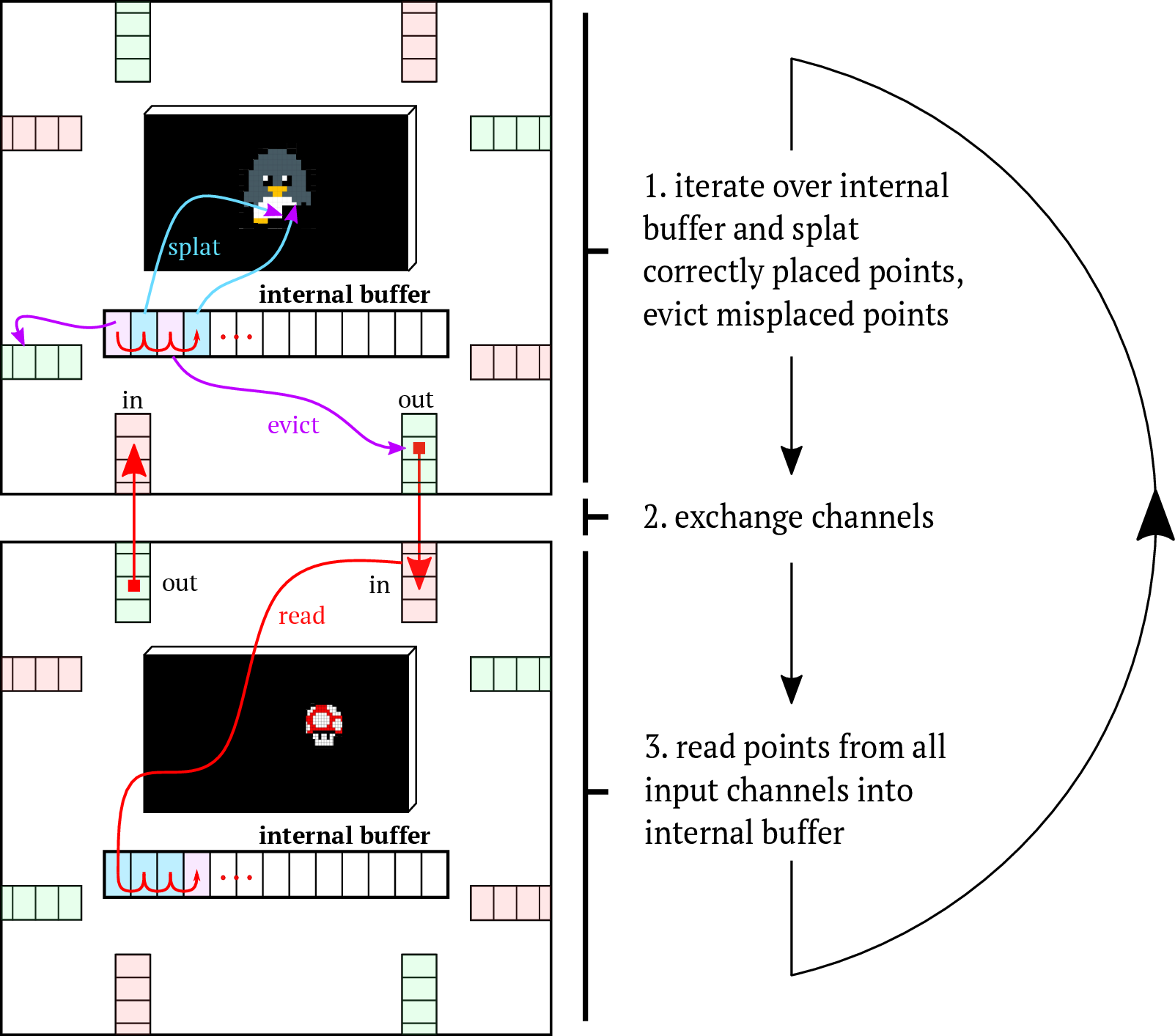
The only host communication per frame is the view/projection matrix (input) and the assembled framebuffer (output). Thus, all scene data remains in on-chip SRAM throughout execution. 1 shows the high-level execution of IPU kernels in the pipeline.
4.2 Framebuffer Partitioning↩︎
The output framebuffer (1280\(\times\)720) is divided into 1,440 equal rectangular slices of 32\(\times\)20 pixels, each pinned to a separate IPU tile’s SRAM. Tiles are arranged in a 2D grid matching the spatial layout of the framebuffer, so that tile adjacency corresponds to screen-space adjacency. Each tile stores its slice as 8-bit RGBX values (2.5 KB per tile). The fourth byte pads each pixel to a 32-bit word boundary, which is required for race-free concurrent writes from multiple hardware threads on the IPU.
4.3 Gaussian Routing via NEWS Grid↩︎
The central challenge of implementing 3DGS on the IPU is distributing Gaussians to the tiles that need them, without a unified address space. On a GPU, any thread can read any Gaussian from global memory which are then allocated to the shared memory of the GPUs SMs (streaming multiprocessor) based on screenspace tile-id. In our IPU implementation, Gaussians must physically migrate through tile-to-tile channels whose connections are fixed at compile time.
Topology.
Tiles are arranged in a 2D mesh ([fig:teaser], middle), with fixed-size channels connecting each tile to its four cardinal neighbours (depicted as small black rectangles on the tile borders). Separate input and output buffers per direction allow simultaneous reads and writes, and boundary tiles wrap their channels back to themselves. This arrangement, inspired by Network-on-Chip routing [24], guarantees that any tile can reach any other through a sequence of single-hop transfers. The design is agnostic to tile count and maps directly to larger grids, a property it shares with wafer-scale architectures [25].
Destination computation.
Each Gaussian has an anchor tile: the tile whose screen region contains the Gaussian’s projected 2D mean. After projection, a tile compares each of its Gaussians against its local screen bounds. Gaussians whose anchors should lie elsewhere are evicted; i.e. written to the outgoing channel that minimises Manhattan distance to the destination.
Routing protocol.
During the exchange phase, each tile’s outgoing buffers are copied to the corresponding incoming buffers of its neighbours. In the subsequent compute phase, tiles read their incoming channels and either store arriving Gaussians locally (if this tile is the destination) or forward them toward the correct destination. This process repeats across BSP supersteps until all Gaussians have reached their anchor tiles. Convergence is guaranteed within \(\max(W, H)\) supersteps, where \(W\) and \(H\) are the grid dimensions.
Each Gaussian carries a unique 32-bit ID assigned at compile time. This ID prevents duplicate storage when a Gaussian passes through intermediate tiles, and setting the ID to zero signals eviction.
4.4 Tree-Pattern ‘Bloom’↩︎
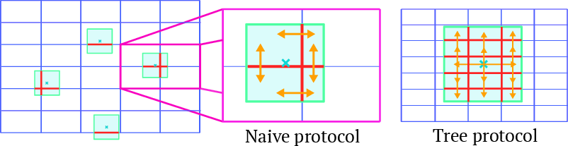
Once a Gaussian reaches its anchor tile, it may still need to be rendered on neighbouring tiles as its 2D screen-space extent can span multiple framebuffer tiles. The GPU implementation handles this by copying into shared memory of each SM that needs it; similarly on the IPU, we must explicitly propagate copies, but we do this using local tile-to-tile communication rather than global memory. This is shown in 2.

We compute the bounding box using the same bounding-radius method as the original 3DGS: three standard deviations of the larger eigenvalue of the 2D covariance define a square bound around each Gaussian’s projected mean. The bounding box determines which neighbouring tiles require a copy. Propagation follows a structured tree pattern: the anchor tile first sends copies along horizontal beams (left/right), then tiles along these beams forward copies vertically (up/down). This ordering eliminates cyclic copying as shown in 3.
| Scene | Blend | Route | Projection | Sort | Total\(_{\max}\) |
|---|---|---|---|---|---|
| Pringles | 17.16 | 1.48 / 3.72 / 14.11 | 3.06 / 3.81 / 11.57 | 0.00 / 0.24 / 3.75 | 46.59 |
| Chairs | 15.76 | 1.60 / 6.82 / 16.06 | 3.10 / 4.41 / 11.73 | 0.00 / 0.40 / 3.86 | 47.41 |
| Salad | 16.66 | 1.48 / 4.14 / 14.22 | 3.07 / 3.95 / 11.61 | 0.00 / 0.26 / 3.37 | 45.86 |
| Sloth | 16.15 | 1.48 / 2.71 / 13.70 | 3.04 / 3.41 / 11.15 | 0.00 / 0.12 / 3.40 | 44.40 |
| Average | 16.43 | 1.48 / 4.35 / 14.52 | 3.07 / 3.90 / 11.52 | 0.00 / 0.26 / 3.60 | 46.07 |
4.5 Rasterisation↩︎
After routing and blooming, each tile holds a set of Gaussians that are visible within its framebuffer region. Rendering proceeds locally:
Culling: Gaussians that land behind the near plane or fall clearly outside the tile are skipped.
Depth sort: The render buffer is sorted by depth using an iterative sort (recursive algorithms are not supported on IPU tiles due to dynamic stack constraints).
Alpha compositing: for each pixel in the local framebuffer slice, contributions from all Gaussians in the sorted render buffer are accumulated in front-to-back order using 1 . The per-pixel colour is computed using the EWA resampling filter, where the exponential falloff from the conic matrix provides the soft Gaussian edges.
Gaussian Representation
Each Gaussian is stored as a 60-byte struct, aligned for efficient IPU memory access:
| Field | Size |
|---|---|
Mean (world space, float3) |
12 B |
Colour (RGB + opacity, float4) |
16 B |
Rotation (quaternion, float4) |
16 B |
Scale (log-space, float3) |
12 B |
Gaussian ID (uint32) |
4 B |
| Total | 60 B |
The byte alignment ensures single-cycle memory reads. View-dependent colour is simplified to a single RGB value per Gaussian (zeroth-order spherical harmonic) to reduce per-primitive memory.

5 Results↩︎
5.1 Experimental Setup↩︎
All experiments are conducted on a single Graphcore Mk2 IPU (GC200) with 1,472 tiles at a framebuffer resolution of 1280\(\times\)720. Standard 3DGS datasets would be too large to fit on-chip [26], [27], so we evaluate on 3D Gaussian maps exported from Gaussian Splatting SLAM [3] trained on real-world RGB sequences. We test on various small scenes of different complexity: Chairs (44K Gaussians), Pringles (91K), Bonsai (273K), Salad (38K), Sloth (25K).
5.2 Memory Budget↩︎
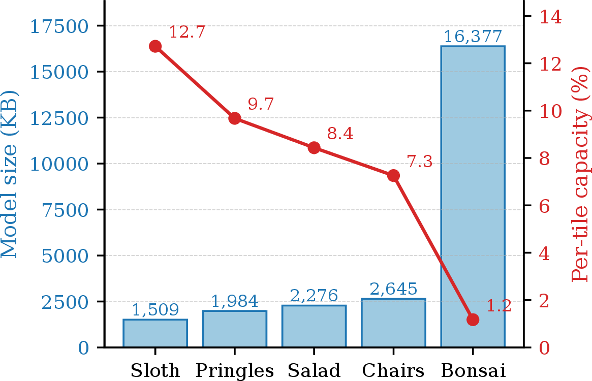
6 summarises the memory footprint of our test scenes. At 60 bytes per Gaussian, model size ranges from 1.5MB for Sloth (25,161 Gaussians) to 16.4MB for Bonsai (272,956). Even the smallest of these is much larger than a single tile’s 192KB Gaussian buffer, which can hold just 12.7% of Sloth and only 1.2% of Bonsai. Copying the scene to every tile, the strategy used by Pupilli [12] for neural path tracing, is therefore not feasible: a whole scene does not fit per tile. Our routing scheme (4.3) addresses this by exploiting the IPU’s aggregate memory instead: Gaussians are distributed only to the tiles that need them, assuming a scene is evenly distributed, then the relevant capacity is 1,472 \(\times\) 192KB rather than the 500KB used in [12]. The approach is well suited to settings such as online SLAM, interactive exploration and AR where the camera moves incrementally rather than teleporting, so each tile’s working set changes only gradually between frames and per-tile occupancy stays within budget.
5.3 Rendered Output↩︎

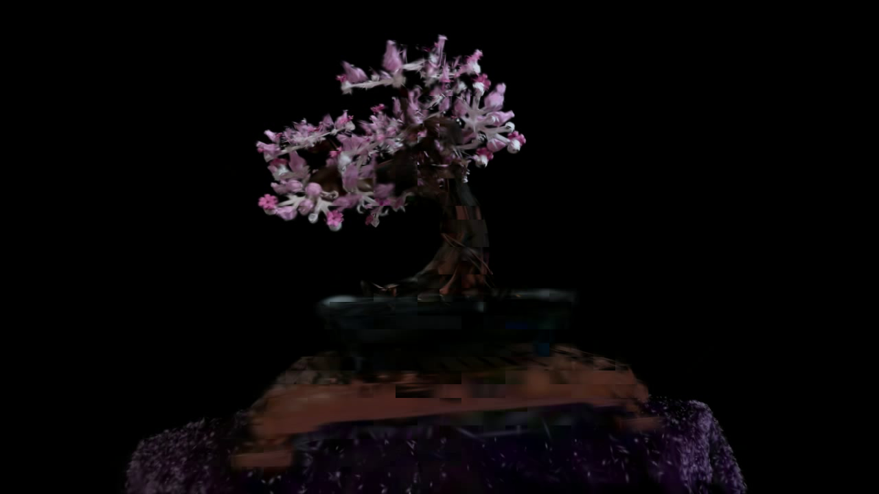

Figure 7: Bonsai scene (272,956 Gaussians). The IPU render captures leaf detail but exhibits tiling artifacts in dense regions where channel saturation prevents full Gaussian propagation. As the Bonsai scene is very dense in certain regions, many of the Gaussians are dropped from the rendering.. a — GPU baseline, b — IPU (ours), c — CPU point cloud
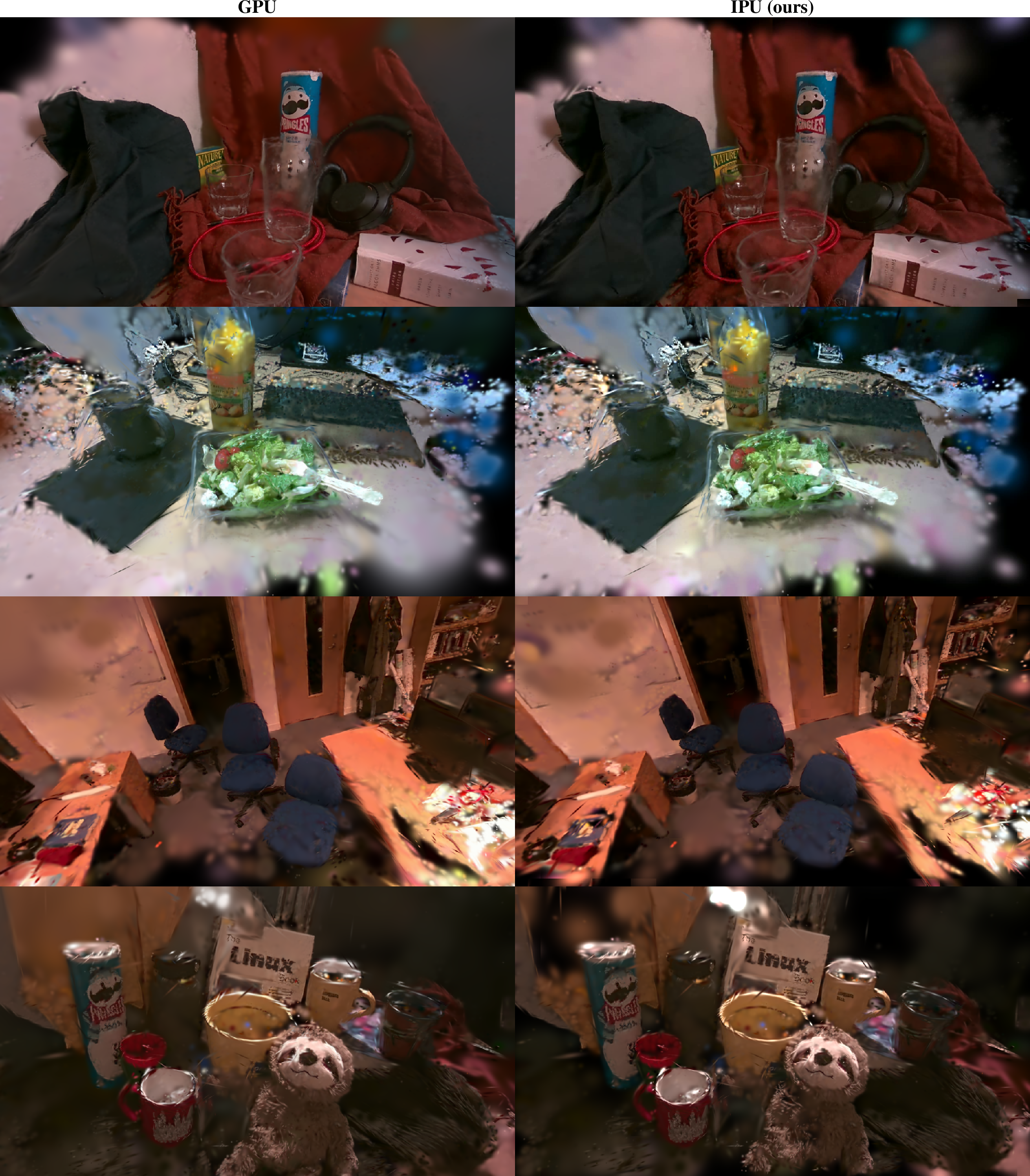
4 shows rendered output compared to the GPU baseline. For these moderate-density scenes the IPU rendering is near-identical to the GPU baseline. The Pringles scene demonstrates that fine details including legible text are preserved. We show also the FPS of the scenes from these viewpoints in 8. Despite the IPU being in no way designed for graphics workloads, the scenes render at reasonable interactive framerates. The dense Bonsai scene in 7 (273K Gaussians) reveals the limits of the current approach: regions of very high Gaussian density exhibit rectangular tiling artifacts (9) caused by channel saturation during the bloom phase. These artifacts are localised to areas where many Gaussians compete for limited channel capacity.


5.4 Host Communication↩︎
Analysis of the execution trace shows that communication between IPU SRAM and the host account for only 1.6% of total execution time. The remaining 98.4% of computation is entirely on-chip, confirming that our approach successfully avoids external memory access for scene data. This contrasts with GPU 3DGS, where DRAM bandwidth is a primary bottleneck, and with the IPU path tracer [12], which streams ray data from the host.
5.5 Power Evaluation↩︎
We measure frame time (ms), power (W) and FPS over 1440 frames (two full orbits of the scene) averaged across four scenes (Sloth, Chairs, Salad, Pringles), reported in 3. An apples-to-apples comparison is challenging as desktop GPUs are optimised for rendering and have far more threads and complex caches. We benchmark a GTX 1080 (40,960 threads, 1.73 GHz) and RTX 4090 (262,144 threads, 2.52 GHz) against the Mk2 IPU (8,832 threads, 1.325 GHz). The setup is identical across chips.
| IPU | GTX 1080 | RTX 4090 | |
|---|---|---|---|
| Frame time (ms) | 50.55 | 1.74 | 0.42 |
| FPS | 19.80 | 580.55 | 2401.47 |
| Power (W) | 27.18 | 74.42 | 89.80 |
| Peak power (W) | 29.30 | 119.67 | 112.61 |
| FPS/W | 0.73 | 7.80 | 26.74 |
| J/frame | 1.373 | 0.128 | 0.037 |
While the IPU underperforms on FPS/W, its power draw is lower and more stable, in a similar range to a Jetson-Orin (7–75 W), suggesting the architecture is suited to low-power deployment. The vendor’s own benchmarks [28] report 571 vs 384 MFLOPS/W for a 16-chip IPU Mk2 pod versus 8\(\times\) A100, attributing this to on-chip SRAM avoiding DRAM transport, specifically \(\sim\)3\(\times\) on data-movement.
5.6 Timing Breakdown↩︎
Using the same setup as 5.5, we measure the execution time of each pipeline stage across tiles (2). The breakdown shows the bottleneck is alpha blending, not routing or inter-tile bandwidth: a single exchange phase is only \(0.07\) ms, confirming that on-chip transfer is fast. As blending is pixel-parallel, more threads per tile would directly increase the framerate.
5.7 Demonstration of Data Locality↩︎
To highlight the reduction in data movement, we move the camera around ‘Sloth’ at different rates and measure the fraction of Gaussians requiring routing per frame (the churn-rate). Static views on the IPU have 0% churn, as Gaussians do not move in memory between frames (4).
| Trajectory | Moved | Churn (%) |
|---|---|---|
| Orbit 0.1\(^\circ\) | 138 | 0.55 |
| Orbit 0.5\(^\circ\) | 616 | 2.45 |
| Orbit 2.0\(^\circ\) | 2,745 | 10.91 |
| Pure translation | 56 | 0.22 |
| Pure rotation 1\(^\circ\) | 1,634 | 11.99 |
| Random teleport | 24,595 | 97.75 |
Churn is much lower for incremental view changes than for teleports, confirming that data movement scales with view-change magnitude. GPU churn is effectively 100% per view, as all Gaussians are potentially reloaded from DRAM (unless cached, which cannot be guaranteed).
5.8 Discussion↩︎
DRAM-Free Constraints
Rendering is highly parallel once each primitive is in the right place, as the alpha compositing is trivially parallel across pixels. The hard part, on both GPUs and the IPU, is getting the data to the tile that needs it. GPUs solve this with a unified global address space and a cache hierarchy: the programmer can treat any Gaussian as locally accessible, and the hardware arranges the transfers. The IPU enables a different solution: local tile-to-tile exchange, structured at compile time. What may look like a different rendering algorithm is really the same algorithm with explicit, software managed data movement. Removing the global address space makes this apparent.
Communication patterns depend on scene content, viewpoint, and Gaussian spatial extent. We show that with sudden view changes the dominant cost is routing; moving Gaussians to the tiles that need them. However, our design allows the algorithm to exploit incremental view changes. We believe the same observation is relevant for algorithm design on a GPU. If routing is the bottleneck, then a GPU with direct inter-SM shared-memory exchange (rather than forcing every cross-SM data movement through DRAM) could cut the dominant cost of GPU 3DGS. This observation is one of the key benefits of stripping away global memory.
IPU vs PPAs
A consequence of the NEWS routing scheme is that Gaussians travel one tile per BSP superstep, which is a latency that can be seen as analogous to data fetching from DRAM. This affects rendering from arbitrary, unrelated viewpoints, but is mostly hidden in the settings with slow viewpoint changes such as scrolling viewers or in online reconstruction. In these settings the camera moves only incrementally between frames, so the set of Gaussians projecting to each tile changes slowly and most primitives are already close to their correct destination. In the case of a GPU, the whole scene is repeatedly fetched from DRAM every new frame and requires caching to be efficient.
Random access through DRAM is only strictly necessary when consecutive views may come from arbitrary camera poses; for incremental view changes, local nearest-neighbour exchange is a natural fit. This is what PPAs exploit to achieve extremely high framerates. Local-only communication has proven performant for front-end vision algorithms (tracking, mapping, incremental reconstruction) and makes exploiting this in differentiable rendering an interesting avenue.
We are transparent about the gap between the IPU and actual pixel processor arrays. IPU tiles have 624 KB of SRAM and can be programmed in C++; PPA pixels have bytes of storage and fixed-function ALUs. Bridging the gap may require:
Compact representations: reducing the 60-byte Gaussian struct to fit PPA-scale memory, perhaps via quantisation or learned compression [29].
Hierarchical approaches: multi-resolution Gaussian representations where coarse levels fit on-sensor and fine detail is deferred.
Hybrid architectures: combining PPA-style sensor-processors for front-end vision with more capable tiles for rendering.
Our work may also be applicable in other settings such as large scale rendering where scene data must be routed between a cluster of many CPUs. Since the IPU is a coarse-grain-reconfigurable-array (CGRA) the techniques we employ could be useful in a number of similar distributed systems such as cloud CPU clusters or Cerebras’ Wafer-Scale-Engine [25], [30].
6 Analysis↩︎
We identify bottlenecks in our DRAM-free implementation for large scenes. As we do not implement any mitigations for these in our prototype, exceeding the preallocated buffer size may compromise both performance and render quality.
1) Inter-tile bandwidth.
The north-east-south-west (NEWS) channels between tiles have fixed capacity defined at compile time. In some cases, when many large Gaussians must be propagated to neighbouring tiles during the bloom phase, the outgoing channels saturate and some copies cannot be forwarded, as in 11. When a Gaussian that spans multiple tiles fails to reach one of them, that tile does not render its contribution, producing a visible hole aligned with the tile boundary. In dense regions where many Gaussians compete for limited channel capacity, these holes are noticeable as rectangular tiling artifacts (9).
2) Propagation latency.
Both routing and bloom operate via local hops on the NEWS grid: a Gaussian can only advance one tile per BSP superstep, and each superstep corresponds to one rendered frame. A Gaussian whose anchor moves \(d\) tiles after a viewpoint change therefore takes \(d\) frames to arrive at its destination. During this transit the Gaussian is absent from the correct tile and may be rendered in the wrong location, producing a visible “blooming” effect where geometry appears to sweep across the screen before settling. The artefact is visible for large camera movements and for Gaussians with large screen-space extent, which must bloom across many tiles after reaching their anchor.
3) Per-tile SRAM capacity.
Each tile must buffer all incoming Gaussians in its 624 KB SRAM. After accounting for the tile’s portion of the framebuffer, the codelet binary and thread stacks, roughly 400 KB remains for scene data. We split this between eight inter-tile channels (one for each of the four NEWS neighbours in each direction, \(\sim\)192 KB total at a capacity of 400 Gaussians per channel) and an internal storage buffer (\(\sim\)192 KB, \(\sim\)3,200 Gaussians). Tiles in dense scene regions can still exceed either budget, causing Gaussians to be dropped; this produces the same holes and rectangular tiling artifacts from 9.
4) Load imbalance.
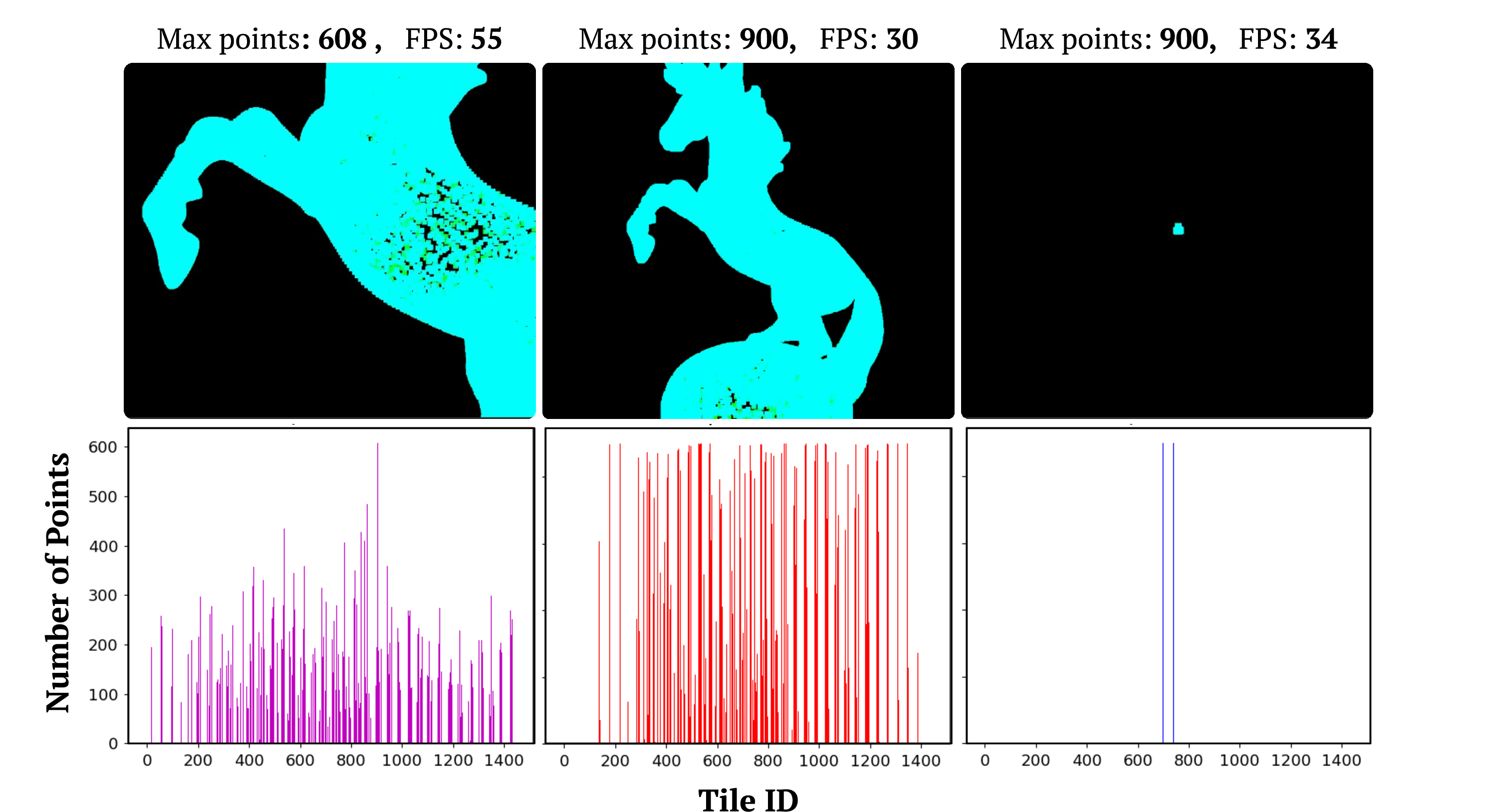
Gaussian density in screen space can be highly non-uniform. In the BSP model, all tiles synchronise at the barrier, so the slowest tile determines the superstep duration. Profiling reveals a high average percentage of execution time is spent waiting for the most loaded tiles to complete. We demonstrate this with the example in 10 where the distribution of Gaussians across tiles changes with viewpoint: a close-up view distributes load relatively evenly, while a distant view concentrates all Gaussians onto a small number of central tiles.

Offloading excess Gaussians to host DRAM, the strategy a GPU manages in hardware, is feasible and would remove artifacts, but we do not implement this to keep computation entirely on-chip. Beyond this, several algorithmic mitigations would reduce the artifacts: 1) bloom only the highest-contribution Gaussians, 2) blend only high-opacity Gaussians, 3) train scenes to be more spatially uniform. We note that there are far fewer artifacts under continuous motion than when teleporting, as most Gaussians are already near their anchor tile. We measure the routing substeps required to converge: a cold-start teleport takes \({\sim}55\) substeps, whereas a small incremental change (a \(1.0\to1.2\times\) zoom) re-converges in only \({\sim}11\). Under the incremental motion typical of SLAM and interactive viewing, the per-frame routing cost stays low.
6.1 Compilation and Memory Allocation↩︎
All these bottlenecks can potentially be alleviated by utilising the idle tiles and exploiting just-in-time compilation for arbitrary tile-to-tile reads at runtime. However, they are interesting to highlight as they can inform the trade-offs of algorithms and representations that better exploit spatial locality of data. The channel/storage split presents an interesting trade-off when choosing buffer sizes: larger channels let more Gaussians propagate per frame (reducing the bloom and tile-boundary artifacts in 9), but leave less room for Gaussians already anchored to the tile, which reduces the detail that can be rendered there. Our current configuration allocates \(\sim\)192 KB to channels and storage; artifacts appear as scenes approach this limit in dense regions, even when the mean per-tile count is far lower.
6.2 Optimisation Opportunities↩︎
The current implementation is a prototype with room for interesting optimisations:
AMP engine: IPU tiles contain a systolic array for matrix products that is not used in our hand-written codelets; exploiting it would accelerate the matrix operations such as projection.
Reduced precision: We use 32-bit precision floating point for Gaussian parameters, this could be compressed to use lower precision as IPU supports FP8 and FP16 which would accelerate the algorithm and help store more Gaussians on-chip.
Exploiting MIMD execution: Unlike GPUs and PPAs, IPU tiles can run entirely different codelets in the same superstep. Our current pipeline treats all tiles uniformly, similar to PPA-style SIMD constraints, but heterogeneous tile roles open interesting possibilities. For example, dedicating peripheral tiles to prefetching and compression while central tiles composite, or using idle tiles in distant-view configurations to run auxiliary work such as feature tracking alongside rendering.
Load balancing: We could detect idle tiles at runtime and offloading projection work to them, exploiting the MIMD flexibility above to shift load dynamically rather than pinning each tile to a fixed screen-space region.
7 Conclusion↩︎
We have presented the first implementation of 3D Gaussian Splatting’s forward pass with only on-chip SRAM. We developed a NEWS grid routing scheme that distributes Gaussian primitives to tiles owning screen-space regions, entirely within the constraints of compile-time-defined communication.
Our implementation shows that 3DGS does not fundamentally require DRAM, once each Gaussian reaches the right tile, rendering is embarrassingly parallel, just as it is on the GPU. What changes is that data movement, normally hardware managed with a global address space and cache hierarchy, becomes a core part of the algorithm: DRAM access is replaced by a network of nearest-neighbour exchanges. Within that network we characterise the following bottlenecks: inter-tile bandwidth, per-tile SRAM capacity, and workload imbalance from non-uniform Gaussian density. Crucially, these bottlenecks are most acute when consecutive viewpoints are far apart, forcing Gaussians to traverse long paths.
A central theme of this work is the exploitation of spatial and temporal locality. Standard GPU 3DGS re-sorts the entire Gaussian list in DRAM on every view change; in contrast, the fabric of the IPU allows us to move data between tiles only when necessary. The insight that motivates such a design is simple: when the viewpoint changes gradually, so does the screen-space projection of the scene, so most primitives remain where they were. Scrolling viewers, real-time game engines, and incremental path tracers all exploit spatial and temporal coherence, yet CUDA implementations of radiance fields do not, and treat every frame as if the camera could teleport. For inverse-graphics applications such as robotics and SLAM, the camera pose is grounded in real 3D motion and cannot jump arbitrarily, making such locality a property we can reliably exploit.
Our experiments suggest that algorithmic choices that exploit data locality pay off on any architecture where the cost of data movement dominates, motivating further work on hierarchical and sparse connectivity patterns. Another natural next step is the backward pass: gradients in an incremental setting, like the Gaussians in the forward pass, would flow primarily between neighbouring tiles, so the same locality argument carries over. In making data movement explicit, the hardware fosters decisions about placement, routing, and load balance of data that motivate further research in the area. We see this as an early step toward rendering pipelines for on-sensor and edge architectures, as well as toward GPU kernels that spend less time waiting on DRAM.
8 Acknowledgements↩︎
This research was partly funded by the EPSRC On-Sensor Computer Vision grant (EP/Y020499/1). We would like to thank Riku Murai, Marwan Taher, Eric Dexheimer, and other members of the Robot Vision Group and Software Performance Optimisation Group for insightful discussions.