More with Less:
a Large Scale Remote Sensing VLM
with a Simple Recipe
July 17, 2026
Abstract
Remote sensing vision-language models are increasingly expected to support open-ended reasoning over Earth Observation data and a variety of tasks. Most recent progress in this area has been driven by remote-sensing-specific architectural designs, often introducing new encoders, alignment modules, or task-specific fusion mechanisms. In this work, we challenge the necessity of such architectural specialization. We show that a generally capable vision-language model can achieve competitive or state-of-the-art performance at challenging remote sensing benchmarks, provided that it is trained at sufficient scale across diverse data and tasks. Our model uses a single language policy that can either answer directly in text or invoke a localization tool for segmentation and grounding. To train this heterogeneous behaviour, we employ a multi-task reinforcement learning framework with adaptive task rewards covering multiple-choice VQA, free-form VQA, captioning, detection, and segmentation across a large variety of input types. Our approach achieves competitive results across a broad set of benchmarks, including high-resolution, multi-temporal, multi-modal and multi-view tasks. Further, as training data scales, our experiments show consistent improvements across most tasks both in and out of distribution, which correlate with per-task data diversity. These findings suggest that, for remote sensing VLMs, data scale is more important than architectural novelty.
1 Introduction↩︎
Remote sensing is becoming central for understanding the Earth at scale. Modern satellite, aerial, and multi-sensor observation systems continuously capture information about land use, urbanization, agriculture, transportation, natural hazards, climate impacts, and environmental change. The resulting imagery is large, heterogeneous, and semantically rich: the same scene may require image-level recognition, fine-grained object localization, pixel-level segmentation, change reasoning, or open-ended question answering. As the volume and diversity of Earth observation data continue to grow, remote sensing increasingly demands models that can move beyond narrow task-specific prediction and support flexible, language-driven interaction with visual and geospatial data.
Recent progress in vision-language models has therefore motivated a new generation of remote sensing large multimodal models [1]–[4]. These systems aim to connect remote sensing imagery with natural language instructions, enabling unified interfaces for tasks such as captioning, visual question answering, grounding, detection, segmentation, and dialogue. A common trend in this literature is to address the peculiarities of remote sensing by designing new remote-sensing-specific architectures, alignment modules, token handling strategies, or modality-fusion mechanisms[3], [5]–[11]. Collectively, these works demonstrate the promise of remote sensing VLMs, but they also reflect a dominant assumption: that progress in the domain requires increasingly specialized model designs.
In this work, we revisit that assumption. Instead of introducing a new remote-sensing-specific architecture, we start from a generally capable vision-language model and scale its remote sensing adaptation through data, tasks, and reinforcement learning (RL). Our central hypothesis is simple: for remote sensing VLMs, broad task coverage and large-scale training data can be more important than architectural novelty. We train a single model across a large and diverse collection of remote sensing datasets and tasks, including free-form visual question answering, captioning, detection, grounding, and segmentation through promptable interaction with SAM3 [12]. To handle the heterogeneity of these tasks, we employ a reinforcement learning strategy with adaptive per-task rewards, allowing the model to optimize across tasks with different output formats and evaluation criteria.
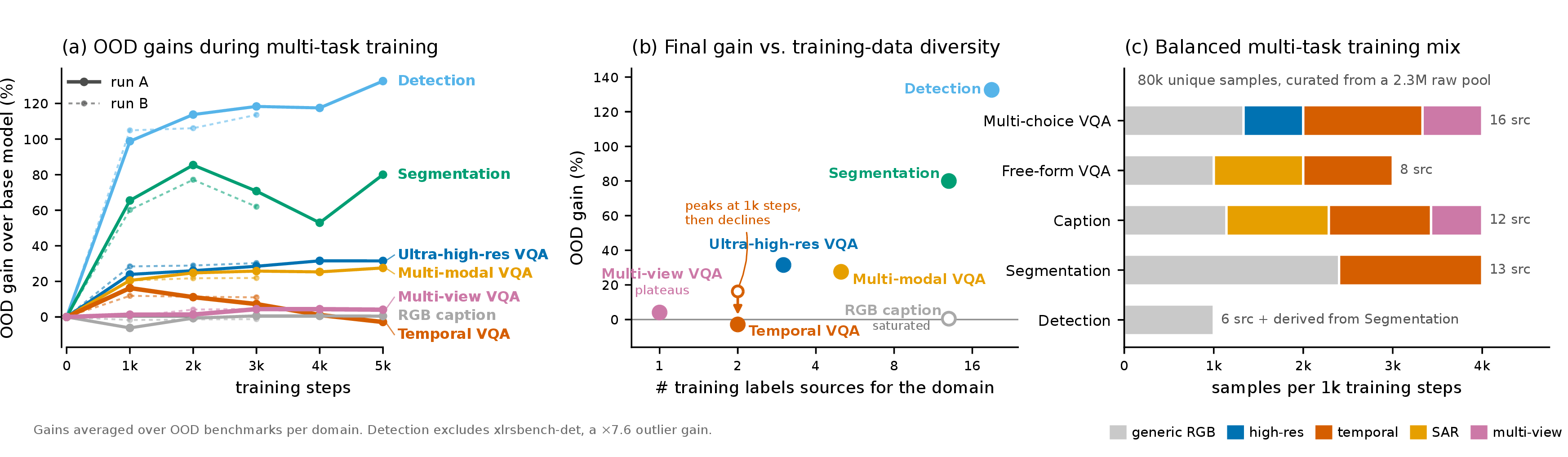
Our results show that this simple recipe is sufficient to achieve competitive or state-of-the-art zero-shot performance across a wide range of remote sensing benchmarks, without modifying the underlying VLM architecture. More importantly, we observe consistent gains as the amount and diversity of training data increase (see Fig. 1), suggesting that remote sensing VLM performance remains strongly data-scalable. These findings shift the emphasis from architecture engineering toward data and task scaling: rather than designing a new model for every remote sensing capability or modality, a strong general VLM can be adapted effectively by exposing it to enough diverse remote sensing supervision and optimizing it with task-aware rewards.
Our contributions can be summarized as follows:
We present More with Less Remote Senser (MLRS), a remote sensing VLM built without introducing any new model architecture. Despite its architectural simplicity, MLRS achieves competitive or state-of-the-art zero-shot performance across a broad range of remote sensing tasks and input types via large-scale multi-task reinforcement learning, demonstrating that a strong general-purpose VLM can be effectively adapted to compete with or surpass specialized VLMs in the remote sensing domain.
We provide an empirical study of data scaling for remote sensing VLMs. Across training data sizes, model sizes, and optimization variants, we find that performance improves with increased data scale and task diversity, suggesting that data-centric scaling is a promising path toward general and capable remote sensing vision-language models.
2 Related works↩︎
| Model | Task Type | Method | Input Type | |||||||||||
| VQA | Cap | Det | VG | Seg | CD | TS | V | RR | MT | MM | UHR | VP | MV | |
| GeoChat [1] | ||||||||||||||
| SkySenseGPT [6] | ||||||||||||||
| LHRS-Bot-nova [7] | ||||||||||||||
| SkyEyeGPT [5] | ||||||||||||||
| TEOChat [13] | ||||||||||||||
| DVLChat [14] | ||||||||||||||
| VHM [2] | ||||||||||||||
| LISAt [15] | ||||||||||||||
| GeoPix [16] | ||||||||||||||
| GeoPixel [17] | ||||||||||||||
| SegEarth-R1 [18] | ||||||||||||||
| SegEarth-R2 [19] | ||||||||||||||
| UniGeoSeg [20] | ||||||||||||||
| Think2Seg-RS [21] | ||||||||||||||
| RemoteReasoner [22] | ||||||||||||||
| RSThinker [23] | ||||||||||||||
| GeoZero [24] | ||||||||||||||
| GeoVLM-R1 [25] | ||||||||||||||
| GeoEyes [26] | ||||||||||||||
| GeoVista [27] | ||||||||||||||
| GeoLLaVA-8K [4] | ||||||||||||||
| LRS-VQA [8] | ||||||||||||||
| UrbanLLaVA [28] | ||||||||||||||
| EarthGPT [29] | ||||||||||||||
| EarthGPT-X [30] | ||||||||||||||
| EarthMaker [10] | ||||||||||||||
| EarthDial [3] | ||||||||||||||
| EarthMind [9] | ||||||||||||||
| TerraScope [31] | ||||||||||||||
| Falcon [32] | ||||||||||||||
| Earth-OneVision [11] | ||||||||||||||
| MLRS (Ours) | ||||||||||||||
10pt
Remote-sensing VLMs. Adapting vision–language models to remote sensing has produced a rapidly growing family of RS-VLMs (see Tab. 1). Early instruction-tuned models such as GeoChat [1], SkySenseGPT [6], and LHRS-Bot [7], [33] established conversational VQA, captioning, and grounding on optical imagery, and subsequent work has expanded coverage along two axes: task and input data types. Along the task axis, models added detection and visual grounding [6], [13], change detection [13], [14], [25], and segmentation [14]–[17], [20], [21]. Along the input axis, dedicated architectures were proposed for multi-temporal sequences (TEOChat [13], DVLChat [14], EarthDial [3]), multi-modal inputs (EarthGPT [29], EarthDial [3], EarthMind [9], TerraScope [31]), ultra-high-resolution scenes (GeoLLaVA-8K [4], LRS-VQA [8], GeoVista [27], GeoPixel [17]), and visual prompting (EarthMaker [10], EarthGPT-X [30]). Multi-view VLMs that merge information from ground views, street panoramas, and satellite imagery, are being developed separately, taking their roots in geolocalization [34], [35], and only recently multi-view models were applied to urban analysis and broader reasoning [28], [36], bringing them closer to remote sensing VLMs. A common thread in these lines of work is that each new input type is addressed with architectural specialization — temporal encoders, modality-specific branches, geometry encoders for visual prompting, or resolution-handling modules. In contrast, we show that a strong general-purpose base model trained on a sufficiently diverse multi-task, multi-domain mixture covers temporal, multi-modal, high-resolution, and multi-view inputs without architectural modification. To our knowledge, our study spans a broader combination of tasks and input types than any prior work.
Post-training paradigms. Most RS-VLMs are trained with supervised fine-tuning alone [1], [3], [6], [7], [13], [14], [29]. However, SFT-trained models tend to fit narrowly to their instruction distributions and degrade on held-out benchmarks — a pattern observed directly both in general [37] and remote sensing [38], [39] domains. A recent wave of reinforcement-learning-based RS-VLMs — RSThinker [23], GeoZero [24], GeoVLM-R1 [25], RemoteReasoner [22], Think2Seg-RS [21], GeoEyes [26], and GeoVista [27] — reports noticeably better generalization, which our evaluation results corroborate. We therefore adopt reinforced reasoning as our post-training strategy.
Segmentation interfaces. RS-VLMs realize segmentation through two interfaces: emitting polygons as text (VHM [2], Falcon [32], Earth-OneVision [11]) or attaching a trained segmentation head [40]–[42] that decodes dense masks (DVLChat [14], UniGeoSeg [20], SegEarth [18], [19], LISAt [15], GeoPix [16], GeoPixel [17], EarthMind [9], TerraScope [31]). Trained dense-mask heads are better suited to remote sensing, where objects are small, numerous, and irregular [43]–[45]. Yet, trained segmentation heads and reinforced reasoning have been so far mutually exclusive: RL-based models either omit segmentation or rely on frozen mask decoders [21], [22]. Our model is the first remote sensing VLM to combine a trained segmentation head with reinforcement learning, via group relative tool optimization (GRTO) [46], obtaining both dense-mask quality and the generalization benefits of RL post-training.
3 Method↩︎
![Figure 2: A single language policy (InternVL [47]) handles all input types — ultra-high-resolution, multi-modal, multi-view, multi-temporal, visual prompting. The policy reasons in text, answers directly, or invokes a SAM3 segmentation tool via a textual prompt; components communicate only through text, with no task-specific encoders or fusion modules. Both components are optimized end-to-end with GRTO [46], using multi-task rewards: embedding similarity for captioning and free-form VQA, box IoU for detection, answer-set IoU for MC-VQA, and mask IoU for segmentation.](/article/2607.15942/visuals/MLRS.png "fig:")
Data scaling. Our central experiment questions what drives generalization in multi-task RS training. We assemble a mixture spanning all multi-choice and free-form VQA, captioning, detection and segmentation (grounded and general) and input types, where by construction the number and heterogeneity of sources backing each domain varies from a single dataset (multi-view) to more than a dozen (segmentation, generic VQA). We then train at scale over an increasing number of unique datapoints while holding the task composition fixed, and periodically evaluate on ID and OOD benchmarks. This design lets us measure how gains evolve with training exposure, and, crucially, whether the shape of each domain’s trajectory — sustained improvement, plateau, or degradation — correlates with the diversity of its training sources rather than with the sheer volume of matching data or initial performance of the model.
The More with Less Remote Senser (MLRS) model. MLRS is a tool-augmented remote sensing VLM that uses a general vision-language model as the central controller and SAM as an external localization tool. The model can operate on Optical, False-colour, SAR imagery, or mixed inputs. SAR observations are represented as grayscale images, allowing them to be processed through the same visual interface as optical images. MLRS also supports multi-image (multi-temporal, multi-view) inputs: when a task provides several images, all of them are shown to the VLM as context, while spatial outputs are produced with respect to the primary image. Finally, visual prompts are straightforwardly overlaid over the primary image.
Given the image or image group and a natural-language instruction, MLRS must decide whether the task requires a direct language response or a spatial prediction. For language-only tasks, such as VQA and captioning, it produces a textual answer. For localization tasks, it instead emits a structured segmentation tool call which describes the target regions using two complementary signals: a noun phrase and one or more bounding boxes, which are passed to SAM3 [12], whose output is filtered through the passed bounding boxes. In this way, the VLM is responsible for semantic grounding and coarse spatial localization, while SAM3 is responsible for producing the final pixel-level mask. This interface is similar in spirit to recent VLM–segmentation-decoder systems for referring segmentation [21], [22], [46], but MLRS uses it as a general remote sensing interface for both textual answering and spatial localization.
This design keeps the VLM architecture unchanged. The model communicates with the segmentation tool only through text: it either answers directly or writes a valid localization call that can be parsed into SAM prompts. Thus, MLRS does not require a specialized remote-sensing architecture or a separate task router. Instead, the VLM itself decides whether to respond in language or invoke the localization tool, enabling a single model to handle captioning, VQA, detection, grounding, and segmentation within the same interface.
Adaptive-reward RL. To fine-tune MLRS, we employ group relative tool optimization (GRTO) [46], where while the VLM is trained with group relative policy optimization (GRPO) [48], a surrogate loss is applied to the tool, SAM3, enabling joint training between policy and tool. We combine binary cross-entropy and semantic IoU for SAM3’s surrogate objective, following [46].
For the GRPO policy objective, we design an adaptive task-dependent reward of the form: \[R = \lambda_{\mathrm{fmt}} F + \lambda_{\mathrm{task}} S,
\label{eq:reward95general}\tag{1}\] where \(F\) is a binary format-validity term, \(S\) is a task-specific score, and we use \(\lambda_{\mathrm{fmt}}=0.1\) and \(\lambda_{\mathrm{task}}=0.9\) during training. The format term encourages the model to use the correct interface: textual tasks must produce an
answer response, while localization tasks must produce a valid segmentation tool call. The score term depends on the task. For multiple-choice VQA, we parse the predicted option set and compute set IoU with the target option set,
supporting both single-answer and multi-answer questions. For free-form VQA and captioning, we compare the extracted answer with the reference using Qwen3-Embedding-0.6B [49], mapping cosine similarity to \([0,1]\). For segmentation, we parse the localization call into phrase-level SAM prompts and score the resulting masks
with semantic IoU against the target masks; if the ground truth contains several masks, we give zero reward if the number of predicted masks does not match, otherwise, we take the mean IoU. For detection, we parse the predicted boxes, convert them to image
coordinates when necessary, greedily match them to ground-truth boxes, and score them by mean matched box IoU. Thus, the same reward template is used across all tasks, while the correctness metric changes according to the required output type. A detailed
definition of each reward component is provided in the appendix. An overview of the framework is shown in Fig. 2.
4 Experiments and results↩︎
4.1 Experimental Design↩︎
Benchmarks. We separate evaluation into in-distribution (ID) and out-of-dis- tribution (OOD) benchmarks. ID benchmarks provide training corpora and held-out test splits to measure task learning on familiar domains: DisasterM3 [50] (bi-temporal optical/SAR disaster imagery; captioning, VQA, and segmentation), DynamicVL [14] (long-range multi-temporal urban scenes; captioning, VQA, and segmentation over optical/SAR images), SARLANG-1M [51] (SAR captioning and free-form VQA), EarthReason [18] (reasoning segmentation), LaSeRS [19] (referring segmentation of varied granularity, multiplicity, linguistic variability, and reasoning requirements), and a held-out split of GeoSeg-1M – GeoSeg-Bench [20] by Ni et al. (visual grounding and reasoning segmentation over Optical and False-colour images). OOD benchmarks share no images or annotations with training and measure generalization across all input types: XLRS-Bench [52] probes Ultra-High-Res. understanding (images up to 10,000×10,000 px), reasoning, and visual prompting; RSHR-Bench [53] adds ultra-high resolution (UHR) MC-VQA with adversarially filtered questions including temporal reasoning; VLRS-Bench [54] targets multi-step complex reasoning over UHR images, understanding and forecasting in multi-temporal scenes, and includes textual and visual prompting; UrBench [36] evaluates multi-view reasoning over paired street-level and satellite imagery; GEOBench-VLM [55] spans all five tasks over multi-modal inputs (RGB, SAR, multi-spectral), and its change-detection subset additionally covers multi-temporal reasoning; and GeoSeg-Bench [56] by Jiang et al. evaluates reasoning segmentation under varied difficulty level – to avoid name collision with ID Benchmarks we refer to it as GeoSeg-Bench2 or GeoSeg2.
Training mix. To study how per-domain data diversity affects generalization, we assemble a multi-task mixture whose domains are deliberately backed by varying numbers of label sources: generic RGB tasks draw on the GeoZero corpus [24] (11 sources for MC-VQA, 8 for captioning, 6 for detection, 4 for free-form VQA) plus GeoLLaVA [4] for high-resolution MC-VQA; segmentation combines GeoSeg-1M [20], LaSeRS [19], EarthReason [18], DynamicVL [14], and DisasterM3 [50] (13 sources); SAR tasks use SARLANG-1M [51] and DisasterM3; multi-temporal tasks rely on only two related sources (DynamicVL, DisasterM3); and multi-view tasks on a single source. We construct multi-view instruction data from CVG-Text [34], a cross-view geo-localization corpus of co-registered ground-level panoramas and satellite views: panorama captions are used directly for captioning, and we deterministically generate two MC-VQA item types — city recognition from a panorama–satellite pair, and cross-view matching, where the model must select which of four satellite views (with same-city hard negatives) depicts the panorama’s location. A total raw pool of collected training data consists of 2.3M image-prompt-answer pairs, we curate an 80k training set from it, balancing task domain and question difficulty if it is provided (see Fig. 1c).
Training setup. We train on eight NVIDIA H200 GPUs with learning rates of \(1\times10^{-6}\) for the VLM and \(1\times10^{-4}\) for SAM3. We use a group size of 8, and a global batch size of 16 unique samples for a total of \(16\times8=128\) rollouts per batch. We set the KL-divergence weight of the GRPO objective to \(\beta=0.01\). For all trainings, we use Low-Rank Adaptation (LoRA) [57] with rank equal to 64. The model is prompted to think, and we set the maximum output length to 1024 tokens. To balance multi-task gradients, we preserve the following composition within each batch: 25% MC-VQA, 25% captioning, 25% free-form VQA and detection, 25% segmentation.
Experiments. To study how data scale affects remote sensing performance when starting from a general-purpose VLM, we train several MLRS variants using the setup described in Section 3. Our primary run uses InternVL3.5-8B [47] as the VLM backbone and is trained with GRTO for 5K steps, corresponding to 80K unique samples. To check run-to-run robustness, we train a second 8B model under the same setup for 3K steps with a different random seed and paraphrased prompt templates. To test whether the observed trends depend on model size, we also train an MLRS variant with the smaller InternVL3.5-2B backbone. We evaluate every checkpoint at 1K-step intervals, allowing us to track performance as the amount of training data increases. Finally, to disentangle the effects of data scaling between the VLM and SAM3, we train an additional 8B model for 5K steps using plain GRPO instead of GRTO, keeping SAM3 frozen. In all runs, the VLM is prompted to reason, decide whether the task requires a textual response or localization, and produce the corresponding output format. The final MLRS model refers to the last checkpoint of the primary 8B GRTO run.
Metrics. We evaluate each task using metrics consistent with the corresponding benchmark whenever possible, introducing alternative metrics only when the original protocol is insufficient for our setting. For tasks with free-form answers, we use dataset-specific LLM-as-judge evaluation [58]. In particular, for DisasterM3 [50], DynamicVL [14], and the VQA split of SARLANG-1M [51], we follow the dataset-specific GPT-style scoring rubrics and prompts. For GEOBench-VLM [55] captioning, we report BERTScore [59], following prior work. For captioning tasks in SARLANG-1M [51] and XLRS-Bench [52], where prior work relies on conventional reference-overlap NLP metrics, we instead reevaluate all baselines with G-Eval [60], a structured LLM-as-judge framework that derives scores from next-token probability distributions rather than a single sampled rating and has been shown to align better with human judgments than reference-overlap metrics. We use Qwen2.5-32B-Instruct [61] as the judge model. For multiple-choice VQA, we report accuracy. For segmentation, we report gIoU, computed as the mean per-sample intersection-over-union. For detection, we report PR@0.5 on GEOBench-VLM [55] and Acc@0.5 on XLRS-Bench [52], following the respective benchmark protocols.
4.2 Results↩︎
| Caption | Free-form VQA | Detection | ||||||||
|---|---|---|---|---|---|---|---|---|---|---|
| 2-6 (lr)7-9 (lr)10-11 Method | DM3 | DVL | SL-1M | XLRS | GEO | DM3 | DVL | SL-1M | GEO | XLRS |
| Qwen | 3.90* | 3.03 | 3.58 | 39.21 | 58.95 | 3.11* | 2.34 | 73.33* | 15.18 | 15 |
| GPT | 2.57 | 4.36 | 10.40 | 47.49 | 64.18 | 3.19 | 2.75 | - | 0.87 | 46 |
| GeoChat | - | - | 6.13 | 3.96 | 43.95 | - | - | - | 11.51 | 14 |
| EarthDial | 1.53 | 1.215 | 12.04 | 11.06 | 53.78 | 2.42 | 1.07 | - | 24.29 | - |
| Base (InternVL) | 1.56 | 2.49 | 9.00 | 44.97 | 37.89 | 2.38 | 0.355 | 25.40 | 23.96 | 5.4 |
| MLRS (InternVL) | 1.54 | 2.80 | 38.24 | 45.92 | 86.88 | 2.27 | 0.810 | 33.20 | 55.74 | 40.9 |
0.53
| Method | DM3 | DVL | RSHR | VLRS | UR | GEO | GEO (chdet) | XLRS |
|---|---|---|---|---|---|---|---|---|
| Qwen | 40.40* | 23.30 | 23.06 | 35.90 | - | 40.0 | 40.05 | 47.40 |
| InternVL | 41.70* | 23.90 | 26.23 | - | 48.80 | 33.3 | 26.23 | 46.20 |
| LLaVA-OneVision | 24.50 | 19.30 | - | - | - | 41.70 | 37.03 | 42.90 |
| GeoChat | 10.70 | - | 32.12 | 33.10 | - | 30.40 | - | 22.9 |
| TEOChat | 23.00 | 17.20 | - | - | - | - | - | - |
| EarthDial | 22.90 | 30.30 | 36.99 | - | - | 37.80 | 42.00 | - |
| DVLChat | - | 33.30* | - | - | - | - | - | - |
| GPT | 42.30 | 34.10 | 44.04 | 43.90 | 61.20 | 41.10 | 44.04 | 38.10 |
| Base (InternVL) | 18.60 | 22.18 | 34.49 | 27.36 | 49.83 | 39.41 | 37.89 | 39.04 |
| MLRS (InternVL) | 20.65 | 22.83 | 29.50 | 23.00 | 51.87 | 50.28 | 46.20 | 51.34 |
0.46
| Method | EarthReason | GeoSeg | LaSeRS | GeoSeg2 | GEO |
|---|---|---|---|---|---|
| LISA | 60.88* | 4.93 | 26.6* | 39.5 | - |
| PixelLM | 60.01* | 4.07 | 29.3* | 0.0 | - |
| PSALM | 68.30* | 64.95* | - | - | - |
| SegEarth-R1 | 70.75* | 66.51* | - | - | - |
| UniGeoSeg | - | 67.75* | - | - | - |
| GlaMM | - | - | 43.6* | 0.0 | 14.11 |
| SegEarth-R2 | - | - | 57.2* | - | - |
| Base (InternVL) | 27.43 | 26.2 | 31.06 | 41.29 | 0.08 |
| MLRS (InternVL) | 67.78 | 47.06 | 66.93 | 69.84 | 15.71 |
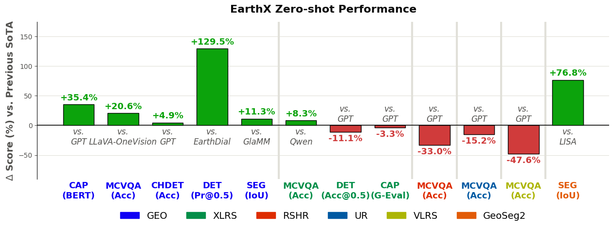
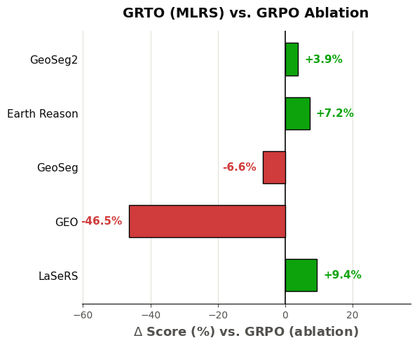
Figure 4: Performance comparisons. (a) Zero-shot performance: percentage difference between MLRS and the best-performing existing baseline for each dataset and task. For every comparison, we report the competing model and the evaluation metric used. (b) GRTO vs. GRPO ablation: IoU percentage difference between MLRS, where SAM3 is fine-tuned (GRTO), and keeping SAM3 frozen (GRPO) for segmentation datasets.. a — Zero-shot performance, b — GRTO vs. GRPO ablation
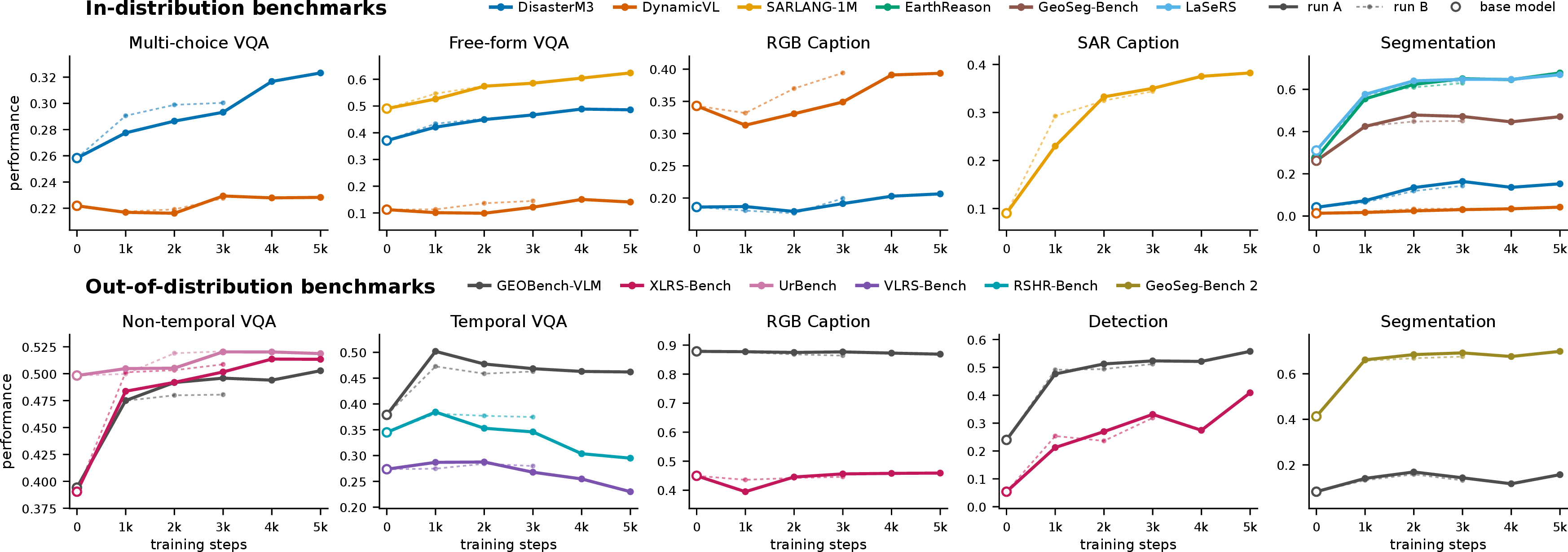
Effects of scaling training data. Fig. 3 reports per-benchmark performance over the course of training for both runs. On in-distribution benchmarks, multi-task training improves majority of task families, with the largest absolute gains where the base model is weakest: SAR captioning rises from 0.09 to 0.38 G-Eval, and referring segmentation improves from 0.27 to 0.68 IoU on EarthReason and from 0.31 to 0.67 gIoU on LaSeRS. Crucially, these gains transfer out of distribution: on held-out benchmarks, detection precision on GEOBench-VLM more than doubles (0.24 → 0.56 Pr@0.5), segmentation improves from 0.41 to 0.70 IoU on GeoSeg-Bench2 and from 0.08 to 0.16 IoU on GEOBench-VLM, and VQA accuracy increases from 0.39 to 0.51 on ultra-high-resolution XLRS-Bench and from 0.39 to 0.50 on GEOBench-VLM (+28%). XLRS-Bench detection improves by a factor of 7.6 (0.054 → 0.409 Acc@0.5). Not all domains benefit equally, however: multi-view VQA on UrBench improves only marginally (0.498 → 0.519) and plateaus after 3k steps, while temporal VQA peaks within the first 1k steps and then degrades, ending below the base model on VLRS-Bench (0.274 → 0.230) and RSHR-Bench (0.345 → 0.295). Captioning metrics on OOD benchmarks remain flat. Finally, the two 8B MLRS GRTO runs track each other closely, suggesting robustness.
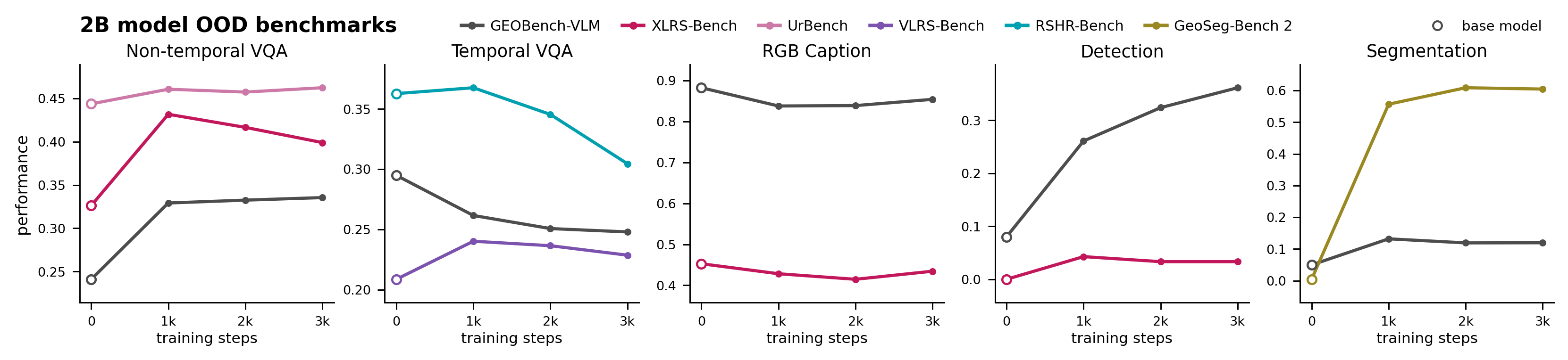
In our 2B backbone ablation, whose OOD performance is visualized in Fig. 5, the trend remains consistent: segmentation and detection continue increasing as data scales, captioning is saturated and remains relatively flat, temporal VQA, hindered by training data diversity, suffers from overfitting, while non-temporal VQA generally increases. The only exception is XLRSBench in non-temporal VQA.
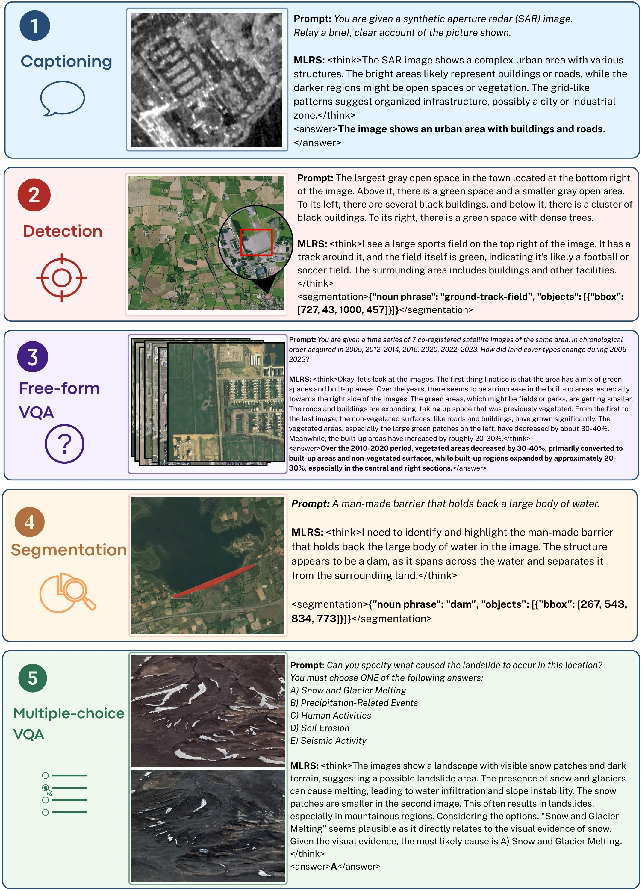
MLRS compared to baselines. We show the performance of MLRS compared to general-purpose and specialized VLMs in Tab. 2 for captioning, free-form VQA and detection, and Tables [tbl:tab:mc-vqa] and [tbl:tab:segmentation] for MC VQA and segmentation. We select the MLRS checkpoint independently of the evaluation curves: the reported model is the final checkpoint of the primary training run, evaluated uniformly across all tasks and benchmarks. In captioning, MLRS ranks first in GEOBench-VLM and second in XLRS-Bench – the two zero-shot benchmarks. In the ID benchmarks, it ranks first in SARLANG-1M, and is surpassed by GPT and Qwen on DisasterM3 and DynamicVL, with a fine-tuned version of Qwen taken for the former. In free-form VQA, MLRS is overshadowed by the much larger GPT and fine-tuned versions of Qwen. In detection – where both datasets are zero-shot – MLRS ranks first in GEOBench-VLM and second in XLRSBench, almost surpassing GPT. In MC VQA, of the six zero-shot benchmarks, MLRS ranks first in three and second in one, failing to reach top-3 only in RSHR and VLRS. Zero-shot, it is once again overshadowed by fine-tuned baselines and GPT. Lastly, in segmentation, MLRS ranks first in both zero-shot benchmarks, first in LaSeRS, third in EarthReason, and fails to reach top-3 only in GeoSeg, where it again loses only to fine-tuned baselines. Overall, MLRS ranks first in 7 OOD benchmarks, second in 3, and fails to reach top-3 only on 2. ID, it tends to be inferior either to GPT, which is much larger, or baselines fine-tuned solely on the corresponding benchmark. Figure 4 (a) compares the zero-shot performance of MLRS with that of the strongest baseline models. Example outputs of MLRS for various tasks are shown in Figure 6.
Effects of data scale on the decoder. Figure 4 (b) compares plain GRPO, where SAM3 is kept frozen, with GRTO, where SAM3 is fine-tuned during reinforcement learning, on the segmentation benchmarks. GRTO improves performance on more benchmarks, indicating that adapting the decoder is generally beneficial. However, the frozen-decoder GRPO variant performs substantially better on the GEOBench-VLM zero-shot benchmark, suggesting that decoder fine-tuning can reduce generalization in some settings. Since GRTO yields gains on the majority of segmentation benchmarks, we use the GRTO-trained model as the final MLRS variant.

5 Discussion↩︎
Scaling and diversifying training data as a path towards state-of-the-art remote sensing. On tasks with the most-diverse sources we observe that improvement over the base model scales well with data, and reaches competitive or state-of-the-art performance. The shape of the learning trajectory appears tied to the diversity of training data available for a domain (Fig. 1b): multi-view VQA, backed by a single source, plateaus at +4%; temporal VQA, backed by only two closely related sources, peaks at +16% after 1k steps and then declines below the base model, consistent with overfitting to a narrow temporal distribution that no longer generalizes; domains backed by three or more heterogeneous sources continue to improve throughout training. Only RGB captioning plateaus because of saturation by base model – no headroom for improvement. Notably, the trends generally do not change when data scaling is applied to a 2B backbone, with the only exception being degrading performance in XLRSBench VQA. Possibly, the 2B model is inherently not powerful enough to process high-resolution images. Overall, this suggests that the results are not dependent on the size of the VLM.
MLRS: all-purpose remote sensing grounded in a general-purpose architecture. The MLRS model achieves top-1 and top-2 results on the majority of benchmarks, except multi-temporal ones, explained by a lack of training data diversity. Baselines outperform MLRS only when trained exclusively on the corresponding benchmark, but never in the OOD setting. The only exception is GPT: a vastly larger general-purpose model. Moreover, GPT is superior on benchmarks for whose annotation it was substantially used itself, i.e. DynamicVL [14], RSHR-Bench [53], XLRS-Bench caption subset [52]; therefore its performance on these benchmarks could be biased. It is also notable that MLRS functions on the largest diversity of input data types and tasks across all baselines.
Fine-tuning sparsely used components must be done with care. Although GRTO fine-tuning of SAM3 improves performance on a majority of segmentation benchmarks, it also leads to a substantial drop on the GEOBench-VLM zero-shot benchmark. This points to a potential overfitting risk when adapting task-specific tools, consistent with the concerns raised in B-GRTO [46]. Unlike the VLM, which is exercised across all tasks and therefore receives broad and diverse supervision, SAM3 is invoked only for localization tasks and is updated using a much narrower subset of the training data. Consequently, whether such components should be fine-tuned depends not only on the amount of available data, but also on the diversity and representativeness of the subset that activates them.
Limitations and future work. This study has several limitations. First, our scaling experiments use backbones from the same model family, since repeating large-scale training across many VLM families is computationally expensive. Evaluating whether the same trends hold for other general-purpose VLMs is an important direction for future work. Second, although we compare against representative set of VLMs designed for remote sensing, architecture- and data-centric approaches are yet to be directly compared under single controlled environment. Third, stronger evidence for the role of data composition would require additional controlled training runs with different data mixtures, but such experiments are costly at the scale considered here. Finally, source count is only a coarse proxy for data diversity. Given the limited number of task domains and the possibility that some domains simply have more room for improvement than others, our diversity-related trends should be interpreted as suggestive rather than conclusive. Future work should quantify intra-domain diversity more directly, for example using effective sample diversity in embedding space, and test whether such measures predict the observed peak-and-decline behavior across domains.
6 Conclusion↩︎
Our findings demonstrate that, given a powerful general-purpose VLM, architectural ingenuity is not necessary to achieve competitive performance in the remote sensing domain. MLRS follows a deliberately simple recipe: retain the architecture of a strong VLM, expose it to a broad mixture of remote sensing tasks and modalities, and train it to decide when to answer directly and when to invoke a localization tool. Despite this simplicity, it achieves competitive or state-of-the-art zero-shot performance across diverse benchmarks, suggesting that strong general VLMs can be effectively adapted to remote sensing through large-scale multi-task training.
More broadly, our results indicate that data scale and task diversity are central drivers of remote sensing VLM performance. As the amount and variety of training data increase, performance continues to improve, supporting a data-centric alternative to increasingly specialized architectural design. At the same time, our experiments show that tool-specific components such as SAM3 should be adapted carefully, since fine-tuning them on narrower subsets can trade in-domain gains for reduced zero-shot generalization. Overall, MLRS points toward a practical path for building general remote sensing VLMs: start from a strong general-purpose model, scale diverse remote sensing supervision, and use simple tool interfaces to extend the model to spatial tasks.
7 Trends analysis↩︎
7.1 Setup, metrics, and covariates↩︎
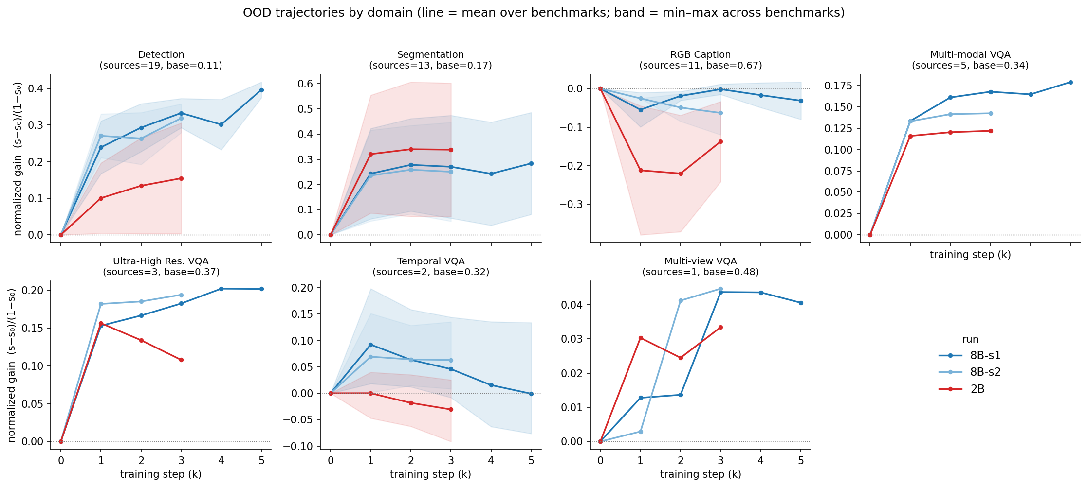
We analyze three training runs: an 8B model trained to 5k steps, a second 8B run with a different random seed trained to 3k steps, and a 2B model trained to 3k steps; all evaluated every 1k steps on the out-of-distribution (OOD) benchmark suite grouped into seven task domains. Unless stated otherwise, statistics are computed at the checkpoint from step 3k.
Gain metric. Benchmarks use heterogeneous metrics and several base-model scores are near zero, our primary measure is the normalized gain \[\Delta_{\mathrm{norm}} = \frac{s_t - s_0}{1 - s_0},\] i.e., the fraction of the remaining headroom recovered by training; all metrics are mapped to \([0,1]\) beforehand. Absolute gains and \(\log\)-ratios (with \(\varepsilon=0.005\)) are used as sensitivity checks and never change the sign of any reported effect.
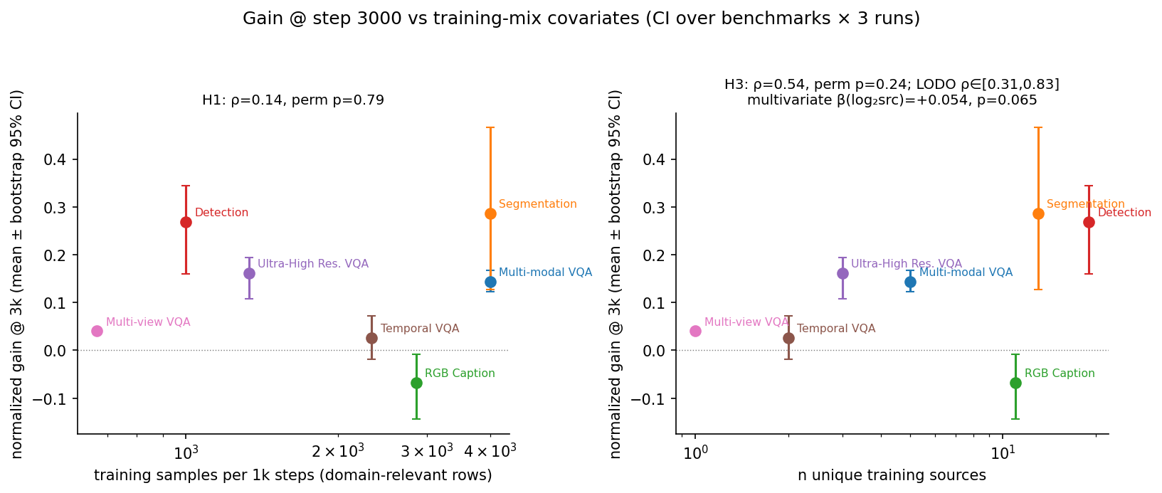
Training-mix covariates. Each OOD domain is matched to the training rows of the same task type and modality. Two covariates are derived per domain: \(n_{\mathrm{smp}}\), the summed number of training samples per 1k steps, and \(n_{\mathrm{src}}\), the number of unique underlying sources of labels (datasets may aggregate several sources). Sources shared across tasks are counted only once; detection additionally inherits the 13 segmentation sources because model produce bounding boxes for both tasks (\(n_{\mathrm{src}}=19\)); and the multi-modal VQA rows intersect heavily at the source level (DynamicVL, DisasterM3, SARLANG1, SARLANG2 contain SAR, GeoSeg-1M contain False-color images), yielding only 5 unique sources despite 16 nominal entries. The resulting counts are: Detection 19, Segmentation 13, RGB Caption 11, Multi-modal VQA 5, Ultra-high-res.VQA 3, Temporal VQA 2, Multi-view VQA 1. We notice, that \(n_{\mathrm{smp}}\) and \(n_{\mathrm{src}}\) are only mildly collinear (\(\rho = 0.39\)).
Domains are not statistically independent: they share underlying sources, and the two 8B runs share initialization. We therefore use permutation tests for all univariate rank correlations, report leave-one-domain-out (LODO) ranges, cluster standard errors by domain in all regressions, and obtain confidence intervals for domain-level means by bootstrap over benchmark\(\times\)run observations within each domain. All visual error bars in Figs. 8–10 are bootstrap 95% CIs unless noted.
We further anayse effect of random seed, model size and base model performance. The hypothesis are: H2 and H1 – behaviour is independent of seed, model size, and \(n_{\text{smp}}\); H3 and H4 – source diversity and base model performance affect behavior.
7.2 H1: Gains are not driven by sampling volume↩︎
We find no evidence that \(n_{\mathrm{smp}}\) predicts per-domain gains (Fig. 8, left). At the domain level (\(n{=}7\)), Spearman \(\rho = 0.14\) (permutation \(p = 0.79\); bootstrap 95% CI \([-0.21, 0.36]\)); Pearson \(r = 0.10\) (\(p = 0.82\)). In the multivariate model of Sec. 7.6, which controls for source diversity and base performance, the coefficient on \(\log_2 n_{\mathrm{smp}}\) is small and non-significant (\(\beta = -0.015\) per SD, \(p = 0.45\)), and remains non-positive in all sensitivity specifications.
7.3 H2: Seed and model scale do not change the behavior↩︎
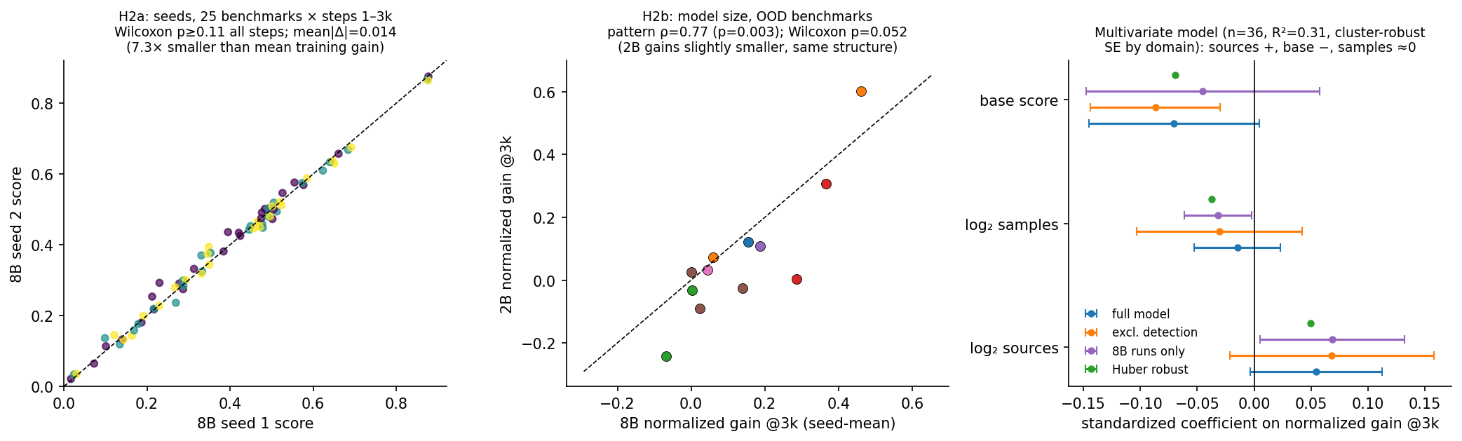
Seed. Comparing the two 8B seeds pairwise over all 25 benchmarks and tasks (Fig. 10a), score differences are not significant at any shared checkpoint (Wilcoxon signed-rank \(p = 0.11\), \(0.43\), \(0.31\) at steps 1k, 2k, 3k), and the mean absolute seed difference (\(0.014\)) is \(7.3\times\) smaller than the mean absolute training gain (\(0.10\)). Per-benchmark normalized gains at 3k are nearly identical across seeds (Spearman \(\rho = 0.965\), \(p < 10^{-6}\)), i.e., not only the magnitudes but the pattern of gains is reproducible.
Model size. The 2B model reproduces the same gain structure as the 8B models on the OOD suite (Fig. 10b): per-benchmark gains correlate at \(\rho = 0.77\) (\(p = 0.003\)) with the seed-averaged 8B gains. The 2B gains are marginally smaller in magnitude (median difference \(-0.048\), Wilcoxon \(p = 0.052\)), driven mainly by detection and ultra-high-resolution VQA (Fig. 7). Trajectory-shape classifications (sustained vs.peaked, Sec. 7.4) agree across seeds and across scales on 57% of domains, with all disagreements occurring in low-amplitude domains where the classification is noise-limited.
We conclude that neither seed nor scale qualitatively alters the mix-dependent behavior, and pool all three runs elsewhere in this analysis.
7.4 H3: Gains and trajectory shape increase with source diversity↩︎
Overall correlation. The domain-level association between gain at 3k and \(n_{\mathrm{src}}\) is positive and moderate (Fig. 8, right): Spearman \(\rho = 0.54\) (permutation \(p = 0.24\) at \(n{=}7\); bootstrap 95% CI \([0.39, 0.64]\); LODO range \([0.31, 0.83]\)). The univariate test is underpowered at seven domains and is additionally confounded by base-model saturation: RGB Caption has 11 sources yet negative gains because its base score is already \(\approx 0.67\) on average. Controlling for base performance, the partial rank correlation remains positive (\(\rho = 0.26\)), and in the multivariate model (Sec. 7.6) \(\log_2 n_{\mathrm{src}}\) carries the largest positive standardized coefficient (\(\beta = +0.054\) per SD, \(p = 0.065\); \(+0.068\) excluding detection; \(+0.050\) under Huber robust regression) — consistently positive across every specification we tried, suggesting significance, however base performance competes for the shared variance. Restricting the analysis to the two 8B runs to remove any model-scale effect strengthens the association: domain-level \(\rho = 0.61\) (permutation \(p = 0.17\); LODO \([0.37, 0.94]\)), and the multivariate sources coefficient becomes significant (\(\beta = +0.069\), \(p = 0.034\)).
Trajectory behaviour. We classify each domain\(\times\)run trajectory using min–max-normalized scores: drop from peak (peak minus final value) and monotonicity (Spearman correlation of score with step). The source-poor domains exhibit the failure mode: Temporal VQA (\(n_{\mathrm{src}}{=}2\)) peaks at step 1/2k and declines in all three runs (mean drop \(0.42\)), and Multi-view VQA (\(n_{\mathrm{src}}{=}1\)) improves only marginally. Tests over the seven domains are directionally consistent but not yet significant (peak retention vs.\(n_{\mathrm{src}}\): \(\rho = 0.52\), permutation \(p = 0.24\); sustained vs.peaked domains, one-sided Mann–Whitney \(p = 0.57\)), again limited by \(n{=}7\) and by RGB Caption, whose decline is saturation-driven rather than diversity-driven. We therefore present the behaviour-type result (Fig. 7) as a qualitative, seed- and scale-reproducible observation rather than a confirmatory finding. The decline in temporal VQA after the peak is yet to be explained by, e.g., effects of forgetting.
7.5 H4: Gains decrease with base-model performance↩︎
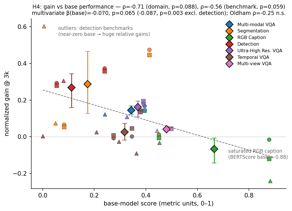
Gains correlate negatively with base performance (Fig. 9): Spearman \(\rho = -0.71\) at the domain level (permutation \(p = 0.088\)) and \(\rho = -0.56\) over the 12 OOD benchmarks (\(p = 0.059\)); in the multivariate model \(\beta_{\mathrm{base}} = -0.070\) per SD (\(p = 0.065\); \(-0.087\), \(p = 0.003\) excluding detection; \(-0.069\) under Huber). However, the effect is not linear, it is rather clearest at the extremes: RGB Caption is saturated at base (BERTScore \(\approx 0.88\); gains \(\approx 0\) or negative in all runs), while detection starts near zero and improves up to \(\times 7.6\) in relative terms. The conservative reading is that base-model headroom is a necessary condition for mix-driven gains.
7.6 Multivariate model↩︎
To disentangle the three covariates we fit, at the benchmark level (12 OOD benchmarks \(\times\) 3 runs, \(n = 36\)), \[\Delta_{\mathrm{norm}}^{(3k)} = \beta_0 + \beta_1 \, z\!\left(\log_2 n_{\mathrm{src}}\right) + \beta_2 \, z\!\left(\log_2 n_{\mathrm{smp}}\right) + \beta_3 \, z\!\left(s_0\right) + \epsilon, \label{eq:mv}\tag{2}\] with standard errors clustered by domain (7 clusters), where \(z(\cdot)\) denotes standardization. Results are shown in Fig. 10c. The model explains \(R^2 = 0.31\) of benchmark-level gain variance with only these three mix/base covariates. Source diversity and base headroom carry comparable, opposite-signed weights, while sampling volume is null — the quantitative counterpart of H1, H3, and H4. Because \(n_{\mathrm{src}}\) and \(s_0\) are themselves anti-correlated in our mix (source-rich domains happen to have low-scoring bases), the two coefficients share variance and each is only marginally significant in the full model; their signs and magnitudes are nevertheless stable across outlier removal and robust estimation.
7.7 Outlier handling and limitations↩︎
Outliers. XLRS-Bench detection (relative gain up to \(\times 7.6\); 2B base score exactly \(0\)) and GeoSeg-Bench2 (2B base \(0.004\)) would dominate any ratio-based analysis; however, the normalized-gain metric \(\Delta_{\text{norm}}\) bounds their influence, and all results were re-checked excluding detection benchmarks and under Huber robust regression, without sign changes.
The main limitations are: statistical power – seven task domains cap the resolution of all domain-level univariate tests, and the behaviour-type association in particular should be treated as observational; the source-sharing dependence between domains, which we mitigate with clustered errors, permutation tests, and LODO; and the collinearity between source diversity and base headroom in this particular mix, which prevents a fully clean attribution between H3 and H4 – a targeted ablation varying \(n_{\mathrm{src}}\) at fixed task type would resolve it. Finally, diversity require stricter measure than number of annotation sources \(n_{\mathrm{src}}\).
8 Detailed Multi-Task Reward↩︎
For each sampled completion, we assign a scalar reward that combines a small format bonus with a task-specific correctness score: \[R = \lambda_{\mathrm{fmt}} F + \lambda_{\mathrm{task}} S, \label{dtyxflab}\tag{3}\] where \(F \in \{0,1\}\) indicates whether the output follows the required interface, \(S \in [0,1]\) is the task-specific score, and we use \(\lambda_{\mathrm{fmt}}=0.1\) and \(\lambda_{\mathrm{task}}=0.9\) during training.
For multiple-choice VQA, the model must answer using the strict
<answer>...</answer> format. The reward supports both letter-based options, such as A, B, and C, and text-based options, such as class names or true/false labels. Let \(\hat{A}\) be the parsed set of predicted options, \(A\) be the target answer set, and \(\Omega\) be the set of valid options. The format term is one only if the
answer can be parsed and all predicted options are valid: \[F^{\mathrm{mc}} = \mathbb{1}\left[ \hat{A} \neq \emptyset \;\wedge\; \hat{A} \subseteq \Omega \right].
\label{eq:mc95format}\tag{4}\] The task score is set IoU between the predicted and target answer sets: \[S^{\mathrm{mc}} = \begin{cases} \dfrac{|\hat{A} \cap A|}{|\hat{A}
\cup A|}, & \text{if } F^{\mathrm{mc}}=1, \\[6pt] 0, & \text{otherwise.} \end{cases} \label{eq:mc95score}\tag{5}\] This handles both single-answer and multi-answer multiple-choice questions.
For free-form VQA and captioning, the model must also produce a non-empty answer inside <answer>...</answer>. Let \(\hat{a}\) be the extracted prediction and \(a\) be the reference. The format term is \[F^{\mathrm{text}} = \mathbb{1}\left[ \hat{a} \text{ is non-empty and correctly enclosed in }
\texttt{<answer>...</answer>} \right]. \label{eq:text95format}\tag{6}\] When the answer is valid, we score it with Qwen3-Embedding-0.6B [49]. The prediction and reference are embedded, last-token pooled, \(\ell_2\)-normalized, and compared with cosine similarity. We map the cosine score
from \([-1,1]\) to \([0,1]\): \[S^{\mathrm{text}} = \begin{cases} \mathrm{clip}_{[0,1]} \left( \dfrac{ 1 + \cos\left(
\phi(\hat{a}), \phi(a) \right) }{2} \right), & \text{if } F^{\mathrm{text}}=1, \\[8pt] 0, & \text{otherwise,} \end{cases} \label{eq:text95score}\tag{7}\] where \(\phi(\cdot)\) denotes the frozen
Qwen3-Embedding-0.6B encoder. This gives a dense semantic reward for open-ended language outputs instead of relying on exact string matching.
For segmentation, the model must invoke the localization tool by producing a valid <segmentation>...</segmentation> call, containing a noun phrase and a list of bounding boxes for each object type. The language output is parsed
into phrase-level prompts, which are passed to SAM to obtain semantic masks. The format term is the validity of this tool call: \[F^{\mathrm{seg}} = \mathbb{1}\left[ \text{the
segmentation tool call is valid and yields SAM masks} \right]. \label{eq:seg95format}\tag{8}\] Let \(\hat{M}=\{\hat{m}^{k}\}_{k=1}^{P}\) be the predicted phrase-level masks and \(M=\{m^{k}\}_{k=1}^{T}\) be the ordered target masks. If the tool call is valid and the number of predicted masks matches the number of target masks, we compute ordered semantic IoU:
\[S^{\mathrm{seg}} = \begin{cases} \dfrac{1}{T} \displaystyle\sum_{k=1}^{T} \mathrm{IoU}\left(\hat{m}^{k}, m^{k}\right), & \text{if } F^{\mathrm{seg}}=1 \text{ and } P=T, \\[12pt] 0,
& \text{otherwise.} \end{cases} \label{eq:seg95score}\tag{9}\] Thus, each predicted semantic mask is compared with the target mask at the same position, and completions that produce the wrong number of masks receive zero segmentation
score. If the task contains only one foreground semantic mask, this reduces to standard mask IoU: \[S^{\mathrm{seg}} = \mathrm{IoU}\left(\hat{m}, m\right).
\label{eq:single95seg95score}\tag{10}\]
For detection, the model uses the same localization interface and outputs the same structured JSON object inside <segmentation>...</segmentation>. The format term is one only when the JSON is valid, contains the required noun
phrase field, and every object contains a valid box: \[F^{\mathrm{det}} = \mathbb{1}\left[ \text{the output is valid localization JSON with valid boxes} \right].
\label{eq:det95format}\tag{11}\] Predicted boxes are converted to image pixels when they are produced in normalized or Qwen-style grid coordinates. Let \(\hat{B}=\{\hat{b}^{p}\}_{p=1}^{P}\) be the predicted
boxes and \(B=\{b^{t}\}_{t=1}^{T}\) be the ground-truth boxes. We greedily match predicted and ground-truth boxes by IoU, using each box at most once, and average over the larger number of predicted and target boxes:
\[S^{\mathrm{det}} = \begin{cases} \dfrac{1}{\max(P,T)} \displaystyle\sum_{(p,t)\in \mathcal{M}} \mathrm{IoU}\left(\hat{b}^{p}, b^{t}\right), & \text{if } F^{\mathrm{det}}=1, \\[12pt]
0, & \text{otherwise,} \end{cases} \label{eq:det95score}\tag{12}\] where \(\mathcal{M}\) is the set of matched prediction–target pairs. Across all tasks, the same reward form in Eq. 1 is used, while the task-specific score \(S\) changes according to the prompt type. This trains the language policy to either answer directly in text or invoke the localization tool when
spatial output is required.
9 Group Relative Tool Optimization↩︎
We use Group Relative Tool Optimization (GRTO) [46] to jointly adapt the language policy and the SAM3 localization tool. Standard tool-use reinforcement learning updates only the policy while keeping the tool fixed. In contrast, GRTO treats the VLM and tool as a coupled system: the VLM learns when and how to call the tool, while the tool is updated on the valid tool calls produced by the VLM.
Let \(\pi_{\theta}\) denote the language policy and \(\psi_{\omega}\) denote the parametrized tool. Both are initialized from pretrained reference models \(\pi_{\theta_0}\) and \(\psi_{\omega_0}\). The goal is to optimize the KL-regularized objective \[J_{\mathrm{KL\text{-}RL}}(\theta,\omega) = \mathbb{E}_{o\sim \pi_{\theta}} \left[ R(o,\psi_{\omega}) \right] - \beta\, D_{\mathrm{KL}}\!\left(\pi_{\theta}\,\|\,\pi_{\theta_0}\right), \label{eq:grto95klrl}\tag{13}\] where \(o\) is a generated completion and \(R\) is the task reward which depends on both policy and tool.
For the policy update, we use the GRPO objective. Given a group of \(G\) completions \(\{o_i\}_{i=1}^{G}\) sampled from the old policy \(\pi_{\mathrm{old}}\), we compute rewards \(\{R_i\}_{i=1}^{G}\), their group mean \(\mu\), and standard deviation \(\sigma\). The relative advantage of completion \(o_i\) is \[A_i = \frac{R_i-\mu}{\sigma}. \label{eq:grto95advantage}\tag{14}\] The policy objective is \[J_{\mathrm{GRPO}}(\theta,\omega_{\mathrm{old}}) = \frac{1}{G} \sum_{i=1}^{G} \sum_{t=1}^{|o_i|} \min\!\left( r_{i,t}A_i, \mathrm{clip}(r_{i,t},1-\epsilon,1+\epsilon)A_i \right) - \beta\, D_{\mathrm{KL}}\!\left(\pi_{\theta}\,\|\,\pi_{\theta_0}\right), \label{eq:grto95grpo}\tag{15}\] where \[r_{i,t} = \frac{ \pi_{\theta}(o_{i,t}\mid o_{i,<t}) }{ \pi_{\mathrm{old}}(o_{i,t}\mid o_{i,<t}) }. \label{eq:grto95ratio}\tag{16}\] The rewards in Eq. 15 are computed using the current frozen copy of the tool, \(\omega_{\mathrm{old}}\), so that the policy update follows the usual clipped GRPO form.
For the tool update, GRTO reuses the same sampled completions. Since the task reward is generally non-differentiable, the tool is optimized with a differentiable surrogate loss \(\mathcal{L}(\psi_{\omega})\) on valid tool calls. The contribution of each rollout is weighted by the stopped-gradient policy likelihood ratio, yielding the GRTO objective \[J_{\mathrm{GRTO}}(\theta,\omega) = J_{\mathrm{GRPO}}(\theta,\omega_{\mathrm{old}}) - \frac{1}{G} \sum_{i=1}^{G} \left( \prod_{t=1}^{|o_i|} r'_{i,t} \right) \mathcal{L}_i(\psi_{\omega}), \label{eq:grto95objective}\tag{17}\] where \(r'_{i,t}=\mathrm{stopgrad}(r_{i,t})\). Thus, the language policy is updated by the GRPO reward signal, while the SAM3 tool is updated through the supervised auxiliary loss induced by the policy-generated tool calls.
SAM3 auxiliary loss. We fine-tune the semantic head of SAM3 using the same BCE + soft-IoU objective as in B-GRTO [46]. For each valid localization call, the VLM produces a noun phrase and bounding box prompts for SAM3. The SAM3 semantic head predicts a foreground logit mask \(\hat{M}\in\mathbb{R}^{H\times W}\), which is converted into a soft probability mask \[S = \sigma(\hat{M}) \in [0,1]^{H\times W}. \label{eq:sam95soft95mask}\tag{18}\] Let \(M\in\{0,1\}^{H\times W}\) be the binary ground-truth foreground mask. The auxiliary segmentation loss is \[\mathcal{L}_{\mathrm{sem}} = \mathcal{L}_{\mathrm{BCE}} + \mathcal{L}_{\mathrm{sIoU}}. \label{eq:sam95sem95loss}\tag{19}\] The binary cross-entropy term is \[\mathcal{L}_{\mathrm{BCE}} = -\frac{1}{HW} \sum_{u=1}^{H} \sum_{v=1}^{W} \left[ M_{uv}\log S_{uv} + (1-M_{uv})\log(1-S_{uv}) \right], \label{eq:sam95bce}\tag{20}\] and the soft-IoU term is \[\mathcal{L}_{\mathrm{sIoU}} = 1 - \frac{ \sum_{u=1}^{H} \sum_{v=1}^{W} S_{uv}M_{uv} }{ \sum_{u=1}^{H} \sum_{v=1}^{W} \left(S_{uv}+M_{uv}-S_{uv}M_{uv}\right) }. \label{eq:sam95siou}\tag{21}\] This loss is applied only to valid localization rollouts, i.e., completions that produce a non-empty, parseable SAM3 prompt with valid bounding boxes. Invalid localization calls and language-only completions do not contribute to the SAM3 auxiliary loss. In our implementation, mask logits are filtered by the VLM-provided bounding boxes before the loss is computed, ensuring that the tool update remains spatially tied to the regions selected by the VLM.
10 Training data mix↩︎
We gather varied set of tasks and modalities: GeoZero corpus [24], consisting of Hard And Instruct parts, for generic RGB; GeoLLaVA [4] for high-res; GeoSeg-1M [20], LaSeRS [19], EarthReason [18] for generic and false-colour segmentation; DynamicVL [14], DisasterM3 [50] for temporal tasks; SARLANG-1M [51] for SAR imagery. SARLANG-1M contains captions and free-form VQA from two sources: text produced from pre-annotated bounding boxes, and text produced from co-registred RGB images – we refer to them as SARLANG1 and SARLANG2. We also construct multi-view instruction data from CVG-Text [34], a cross-view geo-localization corpus of co-registered ground-level panoramas, ground-view captions, and satellite images: panorama captions are used directly for captioning, and we deterministically generate two MC-VQA item types — city recognition from a panorama–satellite pair, and cross-view matching, where the model must select which of four satellite views (with same-city hard negatives) depicts the panorama’s location. A total raw pool of collected training data consists of 2.3M image-prompt-answer pairs. We randomly select a 80k subset to ensure all samples are unique during training. To balance the tasks and sources we utilize the following mix:
Multi-choice VQA: GeoLLaVA, GeoZero Hard, GeoZero Instruct, DynamicVL, DisasterM3, VQA constructed from CVG-text – each 3333 samples;
Free-form VQA: GeoZero Hard, GeoZero Instruct, SARLANG1, SARLANG2, DynamicVL, DisasterM3 – each 2500 samples;
Caption: GeoZero Hard, GeoZero Instruct, SARLANG1, SARLANG2, DynamicVL, DisasterM3, CVG-text – each 2857 samples;
Segmentation: GeoSeg-1M, LaSeRs, EarthReason, DynamicVL, DisasterM3 – each 4000 samples;
Detection: GeoZero Hard, GeoZero Instruct – each 2500 samples.
11 Prompts Used↩︎
During training, we replace dataset-specific prompts with generic task templates to avoid artificially inflating the model’s performance. In particular, we do not want the model to exploit benchmark-specific phrasing as a shortcut for deciding how to answer. However, some datasets contain prompts that become ambiguous in a multi-task setting. For example, certain localization datasets provide only a description of the target object, without explicitly stating whether the object should be segmented or detected. In such cases, we minimally disambiguate the instruction by adding a task cue, such as prepending “Segment the ...”. This reflects the expected deployment setting, where users specify the task they want the model to solve rather than providing only an underspecified statement.
Main MLRS prompt. In addition to the task-specific instruction, we prepend a default system instruction to every prompt seen by the model during both training and inference. This instruction defines the two allowed output modes: a textual answer for language-only tasks and a segmentation tool call for localization tasks, along with their corresponding output formats. Using the same instruction across all settings provides a stable multi-task interface, making the expected behavior explicit and allowing reinforcement learning to focus on improving task performance rather than discovering the output protocol from scratch.
You are solving visual reasoning tasks.
You may respond in one of two final formats:
1. If the task requires segmenting/localizing objects in the image, call the segmentation tool by outputting:
<segmentation>{"noun phrase": "...", "objects": [{"bbox": [x1, y1, x2, y2]}]}</segmentation>
The segmentation JSON must contain:
- "noun phrase": exactly one referential noun phrase identifying the target.
- "objects": a list of objects, each with one "bbox" field.
- Coordinates should use the 0-999 image coordinate grid.
If the task includes several images, segmentation tool uses the last rgb image.
2. If the task asks for a textual answer and does not require segmentation, output:
<answer>your textual answer</answer>
Use <think>...</think> before the final tag when reasoning is useful.
Do not use <answer> for segmentation. Do not use <segmentation> for non-segmentation answers.
G-Eval prompt for captioning.
You are an expert judge evaluating satellite image captions. Your task is to compare the Predicted caption against the Ground Truth (GT) and assign a score based on object accuracy, counting, and hallucinations.
Evaluation Steps:
1. Analyze the Ground Truth for core objects and counts.
2. Check the Prediction for "Imaginary Objects" (Hallucinations) not present in the GT.
3. Verify if object counts and spatial relationships match the GT.
4. Assign a strict score from 1-5 using the rubric below.
Scoring Rubric:
1 (Critical Failure): Major hallucination (imaginary objects) or completely wrong scene classification.
2 (Poor): Correct scene type, but severe errors in object counting or wrong object attributes.
3 (Fair): Captures the main gist, but has minor hallucinations or noticeable counting errors.
4 (Good): Accurate objects and counts, with only very minor semantic differences or missing fine details.
5 (Perfect): Exact match in object types, counts, and spatial layout with no hallucinations.
Input:
Ground Truth: {gt}
Predicted: {pred}
Score:
Where we insert the ground truth and provided captions in place of {gt}, and {pred} respectively.
G-Eval prompt for free-form VQA.
You are an expert judge evaluating Visual Question Answering (VQA) outputs. Your task is to compare the Predicted Answer against the Ground Truth (GT) Answer for the given Question and assign a score based on factual correctness, completeness, and hallucinations.
Evaluation Steps:
1. Analyze the Question to understand what information is required.
2. Examine the Ground Truth Answer for key facts, values, and constraints.
3. Check the Predicted Answer for hallucinations (information not supported by the GT).
4. Verify correctness, precision, and completeness of the Predicted Answer.
5. Assign a strict score from 1-5 using the rubric below.
Scoring Rubric:
1 (Critical Failure): Incorrect answer or major hallucination; does not address the question.
2 (Poor): Partially related but mostly incorrect; major factual errors or missing key elements.
3 (Fair): Captures the general idea but contains minor errors, ambiguity, or incomplete details.
4 (Good): Mostly correct and complete; only very minor inaccuracies or omissions.
5 (Perfect): Exact match with the Ground Truth; fully correct, precise, and no hallucinations.
Input:
Question: {q}
Ground Truth Answer: {gt}
Predicted Answer: {pred}
Score:
Where we insert the question, ground truth, and provided answer in place of {q}, {gt}, and {pred} respectively.
12 Per-sub-task results↩︎
Several benchmarks provide fine split on reasoning and sub-tasks dimensions, therefore we report according performance of our base model and MLRS model, see Tables 3, 4, 5, ¿tbl:tab:pt95ur?, 6, 7.
| Method | Perception | Reasoning | ||||||||||||
|---|---|---|---|---|---|---|---|---|---|---|---|---|---|---|
| Sub-tasks (L-3) | OC | RC | OLUC | RLUC | OCC | OCL | OMS | OSR | AD | ECR | RP | RCCD | CCR | Avg. |
| Remote Sensing MLLMs | ||||||||||||||
| GeoChat | 16.7 | 29.0 | 2.0 | 23.0 | 21.1 | 16.8 | 35.0 | 24.2 | 33.0 | 43.0 | 10.0 | - | 21.0 | 22.9 |
| Closed-source MLLMs | ||||||||||||||
| GPT-4o | 25.0 | 32.0 | 15.0 | 66.0 | 9.5 | 11.3 | 11.7 | 24.6 | 73.0 | 73.0 | 35.0 | 20.0 | 25.0 | 32.4 |
| GPT-4o-mini | 23.3 | 25.0 | 19.0 | 59.5 | 40.9 | 31.0 | 65.0 | 23.6 | 71.0 | 71.0 | 29.0 | 6.7 | 30.0 | 38.1 |
| Claude 3.7 Sonnet | 27.6 | 22.7 | 17.4 | 68.4 | 30.5 | 29.9 | 63.6 | 27.6 | 64.8 | 78.4 | 34.5 | 27.8 | 32.6 | 40.5 |
| Gemini 2.0 Flash | 41.7 | 45.0 | 38.0 | 73.5 | 34.6 | 27.6 | 61.7 | 32.0 | 73.0 | 82.0 | 43.0 | 30.0 | 51.0 | 48.7 |
| Open-source MLLMs | ||||||||||||||
| InternLM-XComposer-2.5 | 21.7 | 42.0 | 7.0 | 68.0 | 31.8 | 27.8 | 6.7 | 26.0 | 72.0 | 81.0 | 41.0 | 36.7 | 47.0 | 39.1 |
| LLaVA-Next | 26.7 | 40.0 | 5.0 | 67.0 | 28.8 | 32.8 | 66.7 | 30.0 | 69.0 | 78.0 | 27.0 | 35.0 | 36.0 | 41.7 |
| LLaVA-OneVision-7B | 25.0 | 38.0 | 2.0 | 69.5 | 35.9 | 35.3 | 65.0 | 25.2 | 76.0 | 83.0 | 24.0 | 43.3 | 36.0 | 42.9 |
| InternVL3-8B | 40.0 | 39.0 | 10.0 | 71.5 | 44.5 | 30.8 | 65.0 | 25.2 | 77.0 | 82.0 | 36.0 | 21.7 | 50.0 | 45.6 |
| Qwen2-VL-7B | 26.7 | 40.0 | 11.0 | 73.0 | 35.9 | 34.6 | 61.7 | 31.8 | 70.0 | 81.0 | 35.0 | 46.7 | 48.0 | 45.8 |
| LLaVA-OneVision-72B | 33.3 | 38.0 | 15.0 | 72.5 | 36.3 | 36.3 | 66.7 | 35.6 | 74.0 | 83.0 | 28.0 | 36.7 | 43.0 | 46.0 |
| InternVL2.5-8B | 38.3 | 37.0 | 10.0 | 77.0 | 33.4 | 35.5 | 65.0 | 21.6 | 73.0 | 83.0 | 34.0 | 50.0 | 43.0 | 46.2 |
| Qwen2.5-VL-7B | 33.3 | 40.0 | 31.0 | 77.0 | 40.6 | 40.5 | 66.7 | 36.2 | 68.0 | 72.0 | 27.0 | 38.3 | 45.0 | 47.4 |
| InternVL3-78B | 23.3 | 49.0 | 33.0 | 74.0 | 42.5 | 37.4 | 66.7 | 30.0 | 76.0 | 81.0 | 40.0 | 45.0 | 42.0 | 49.2 |
| Qwen2.5-VL-72B | 33.3 | 47.0 | 39.0 | 80.0 | 45.3 | 42.1 | 65.0 | 34.0 | 71.0 | 74.0 | 37.0 | 43.3 | 42.0 | 50.2 |
| Base | 21.7 | 20.0 | 48.0 | 50.5 | 30.1 | 33.1 | 63.3 | 23.4 | 54.0 | 71.0 | 38.0 | 23.3 | 31.0 | 39.0 |
| MLRS | 38.3 | 39.0 | 47.0 | 78.0 | 35.8 | 33.5 | 66.7 | 31.8 | 70.0 | 80.0 | 52.0 | 43.3 | 52.0 | 51.3 |
| Model | Perception | Avg. | Reasoning | Avg. | Multi-turn | |||||||||||||||
|---|---|---|---|---|---|---|---|---|---|---|---|---|---|---|---|---|---|---|---|---|
| 2-10(lr)12-16(lr)18-20 | COL | SHP | DET | OC | REL | OGD | RG | OCN | RCN | AD | FP | MRJC | MRJCS | OSJ | MAD | MTFP | MOSJ | |||
| Remote Sensing VLMs | ||||||||||||||||||||
| EarthDial | 41.0 | 22.0 | 21.0 | 30.0 | 32.5 | 30.5 | 27.1 | 18.0 | 31.0 | 28.1 | 42.0 | 30.0 | 29.5 | 32.0 | 52.0 | 37.1 | 56.7 | 60.0 | 73.5 | 63.4 |
| GeoChat | 32.5 | 22.0 | 24.0 | 29.5 | 40.0 | 25.0 | 22.9 | 22.5 | 29.0 | 25.9 | 30.0 | 24.0 | 25.5 | 30.0 | 32.0 | 28.3 | 48.3 | 46.0 | 62.9 | 52.4 |
| GeoLLaVA-8K | 25.0 | 24.0 | 25.0 | 25.0 | 25.0 | 25.0 | 21.4 | 25.0 | 25.0 | 24.5 | 24.0 | 0.0 | 0.0 | 34.0 | 22.0 | 16.0 | 25.0 | 24.7 | 47.7 | 32.5 |
| VHM | 25.5 | 25.0 | 26.0 | 26.5 | 55.0 | 25.0 | 22.9 | 25.0 | 25.0 | 25.7 | 26.0 | 24.0 | 26.5 | 34.0 | 28.0 | 27.7 | 45.0 | 53.3 | 46.2 | 48.2 |
| Open-source VLMs | ||||||||||||||||||||
| InternVL2.5-8B | 25.5 | 22.0 | 26.0 | 26.0 | 22.5 | 24.5 | 30.0 | 22.5 | 20.0 | 24.3 | 26.0 | 20.0 | 22.5 | 34.0 | 20.0 | 24.5 | 25.0 | 28.7 | 35.6 | 29.8 |
| InternVL3.5-8B | 21.5 | 28.0 | 18.0 | 21.5 | 29.0 | 28.5 | 30.0 | 26.5 | 25.0 | 25.3 | 20.0 | 16.0 | 29.0 | 34.0 | 26.0 | 25.0 | 30.0 | 22.7 | 40.2 | 31.0 |
| MiniCPM2_6 | 21.5 | 28.0 | 30.0 | 24.0 | 19.5 | 29.5 | 34.3 | 22.0 | 29.0 | 27.4 | 26.0 | 30.0 | 35.0 | 32.0 | 30.0 | 30.6 | 26.7 | 23.3 | 31.1 | 27.0 |
| Phi-3.5-Vision | 25.0 | 24.0 | 25.0 | 25.0 | 23.5 | 25.0 | 22.9 | 25.0 | 25.0 | 24.5 | 24.0 | 22.0 | 23.5 | 30.0 | 22.0 | 24.3 | 28.3 | 24.7 | 47.0 | 33.3 |
| Qwen2.5-VL-7B | 29.5 | 25.0 | 22.0 | 28.0 | 25.0 | 24.5 | 24.3 | 26.5 | 22.0 | 25.2 | 26.0 | 28.0 | 25.0 | 10.0 | 20.0 | 21.8 | 21.7 | 24.0 | 10.6 | 18.8 |
| Deepseek-VL | 22.5 | 22.0 | 21.0 | 25.0 | 20.5 | 26.0 | 28.6 | 20.5 | 22.0 | 23.1 | 22.0 | 28.0 | 50.0 | 32.0 | 20.0 | 30.4 | 20.0 | 23.3 | 33.3 | 25.5 |
| VILA-HD | 40.0 | 22.0 | 22.0 | 37.0 | 35.5 | 26.0 | 21.4 | 24.5 | 24.0 | 28.0 | 58.0 | 30.0 | 55.0 | 32.0 | 58.0 | 46.6 | 65.0 | 57.3 | 57.6 | 60.0 |
| Closed-source VLMs | ||||||||||||||||||||
| GPT5 | 29.0 | 10.0 | 23.0 | 23.0 | 37.0 | 24.5 | 31.4 | 20.0 | 23.0 | 24.5 | 74.0 | 58.0 | 35.0 | 34.0 | 66.0 | 53.4 | 78.3 | 73.3 | 86.4 | 79.3 |
| GPT-4o | 49.5 | 23.0 | 15.0 | 35.5 | 30.5 | 28.0 | 27.1 | 22.5 | 41.0 | 30.2 | 68.0 | 56.0 | 30.5 | 32.0 | 64.0 | 50.1 | 70.0 | 72.0 | 84.1 | 75.4 |
| GPT-4o-mini | 41.5 | 16.0 | 29.0 | 31.5 | 31.5 | 32.0 | 28.6 | 19.5 | 32.0 | 29.1 | 54.0 | 54.0 | 31.5 | 48.0 | 54.0 | 48.3 | 78.3 | 68.0 | 75.0 | 73.8 |
| Gemini-2.5-pro | 55.0 | 18.0 | 31.0 | 40.0 | 41.5 | 32.5 | 45.7 | 25.0 | 25.0 | 34.9 | 66.0 | 32.0 | 41.5 | 38.0 | 50.0 | 45.5 | 56.7 | 60.0 | 57.6 | 58.1 |
| Base | 50.5 | 35.0 | 27.0 | 36.0 | 26.0 | 22.0 | 22.9 | 12.0 | 43.0 | 30.5 | 60.0 | 14.0 | 10.0 | 12.0 | 58.0 | 30.8 | 41.3 | 66.7 | 50.0 | 52.7 |
| Best eval (1k step) | 46.5 | 24.0 | 27.0 | 34.0 | 30.5 | 37.5 | 35.7 | 24.5 | 41.0 | 33.5 | 56.0 | 24.0 | 30.0 | 38.0 | 48.0 | 37.0 | 40.0 | 66.7 | 50.0 | 35.7 |
| MLRS (5k step) | 48.0 | 30.0 | 9.0 | 30.5 | 16.5 | 24.5 | 10.0 | 21.0 | 38.0 | 25.3 | 44.0 | 10.0 | 30.0 | 30.0 | 38.0 | 30.4 | 30.0 | 55.3 | 36.7 | 40.7 |
| Models | Cognition | Decision | Prediction | Avg. Score. | |||||||||||
|---|---|---|---|---|---|---|---|---|---|---|---|---|---|---|---|
| 2-9 (lr)10-11 (lr)12-15 | CR | CFR | SIR | MIR | ST-CFR | ST-CCR | ST-ER | ST-CR | PR | ER | ST-CS-PR | ST-M-PR | ST-SU-PR | ST-SQ-PR | |
| General MLLMs | |||||||||||||||
| GPT-5.4 | 0.412 | 0.416 | 0.516 | 0.516 | 0.416 | 0.384 | 0.436 | 0.416 | 0.456 | 0.484 | 0.424 | 0.384 | 0.400 | 0.416 | 0.439 |
| GPT-5-chat | 0.424 | 0.400 | 0.472 | 0.316 | 0.276 | 0.352 | 0.380 | 0.368 | 0.388 | 0.388 | 0.388 | 0.276 | 0.280 | 0.292 | 0.356 |
| GPT-4o-2024-11-20 | 0.376 | 0.432 | 0.420 | 0.332 | 0.360 | 0.352 | 0.400 | 0.364 | 0.286 | 0.334 | 0.416 | 0.352 | 0.284 | 0.340 | 0.361 |
| GPT-4o-mini | 0.428 | 0.416 | 0.428 | 0.328 | 0.400 | 0.356 | 0.352 | 0.336 | 0.248 | 0.304 | 0.424 | 0.372 | 0.280 | 0.304 | 0.355 |
| Gemini-3.1-Pro-Preview | 0.420 | 0.448 | 0.496 | 0.396 | 0.476 | 0.436 | 0.460 | 0.456 | 0.428 | 0.458 | 0.400 | 0.360 | 0.428 | 0.432 | 0.436 |
| Gemini-2.5-flash | 0.200 | 0.188 | 0.264 | 0.240 | 0.188 | 0.160 | 0.116 | 0.160 | 0.232 | 0.240 | 0.164 | 0.168 | 0.116 | 0.152 | 0.190 |
| Claude-3.5-haiku | 0.308 | 0.316 | 0.304 | 0.360 | 0.192 | 0.208 | 0.232 | 0.200 | 0.372 | 0.370 | 0.208 | 0.224 | 0.248 | 0.168 | 0.270 |
| Claude-Opus-4.6 | 0.272 | 0.264 | 0.372 | 0.408 | 0.452 | 0.392 | 0.336 | 0.300 | 0.398 | 0.348 | 0.264 | 0.320 | 0.396 | 0.340 | 0.350 |
| Grok-2-vision | 0.188 | 0.216 | 0.288 | 0.368 | 0.232 | 0.240 | 0.240 | 0.280 | 0.252 | 0.300 | 0.220 | 0.196 | 0.172 | 0.148 | 0.240 |
| 1-1 (lr)2-9 (lr)10-11 (lr)12-15 (lr)16-16 Deepseek-vl2 | 0.372 | 0.392 | 0.452 | 0.344 | 0.144 | 0.216 | 0.200 | 0.148 | 0.416 | 0.446 | 0.096 | 0.128 | 0.064 | 0.080 | 0.250 |
| GLM-4.5v | 0.268 | 0.136 | 0.248 | 0.312 | 0.152 | 0.084 | 0.084 | 0.132 | 0.312 | 0.340 | 0.132 | 0.172 | 0.180 | 0.112 | 0.190 |
| LLama-3.2-11B | 0.232 | 0.228 | 0.244 | 0.264 | - | - | - | - | 0.292 | 0.286 | - | - | - | - | 0.110 |
| LLama-3.2-90B | 0.368 | 0.364 | 0.356 | 0.308 | 0.236 | 0.268 | 0.300 | 0.268 | 0.408 | 0.430 | 0.308 | 0.352 | 0.268 | 0.212 | 0.318 |
| Qwen2.5-VL-7B | 0.256 | 0.172 | 0.384 | 0.176 | 0.224 | 0.324 | 0.248 | 0.216 | 0.198 | 0.238 | 0.328 | 0.280 | 0.232 | 0.212 | 0.249 |
| Qwen2.5-VL-32B | 0.292 | 0.312 | 0.368 | 0.296 | 0.244 | 0.300 | 0.256 | 0.236 | 0.370 | 0.308 | 0.276 | 0.284 | 0.236 | 0.156 | 0.281 |
| Qwen2.5-VL-72B | 0.216 | 0.300 | 0.296 | 0.392 | 0.316 | 0.240 | 0.216 | 0.204 | 0.402 | 0.370 | 0.172 | 0.180 | 0.204 | 0.188 | 0.264 |
| Qwen3-VL-2B | 0.350 | 0.361 | 0.468 | 0.185 | 0.204 | 0.428 | 0.412 | 0.336 | 0.287 | 0.260 | 0.380 | 0.312 | 0.304 | 0.312 | 0.330 |
| Qwen3-VL-8B | 0.341 | 0.363 | 0.472 | 0.211 | 0.388 | 0.405 | 0.398 | 0.371 | 0.233 | 0.275 | 0.381 | 0.401 | 0.401 | 0.384 | 0.359 |
| Qwen3-VL-32B | 0.372 | 0.416 | 0.476 | 0.316 | 0.408 | 0.428 | 0.388 | 0.392 | 0.416 | 0.364 | 0.388 | 0.456 | 0.336 | 0.372 | 0.395 |
| Remote Sensing MLLMs | |||||||||||||||
| GeoChat | 0.280 | 0.332 | 0.360 | 0.308 | - | - | - | - | 0.352 | 0.356 | - | - | - | - | 0.331 |
| VHM | 0.302 | 0.297 | 0.308 | 0.210 | - | - | - | - | 0.324 | 0.332 | - | - | - | - | 0.296 |
| ScoreRS w/ SFT | 0.403 | 0.367 | 0.421 | 0.345 | 0.294 | 0.310 | 0.288 | 0.284 | 0.382 | 0.419 | 0.341 | 0.320 | 0.313 | 0.295 | 0.347 |
| ScoreRS w/ RL | 0.313 | 0.338 | 0.382 | 0.295 | 0.399 | 0.335 | 0.367 | 0.392 | 0.409 | 0.371 | 0.338 | 0.313 | 0.382 | 0.342 | 0.355 |
| Base | 0.300 | 0.300 | 0.300 | 0.316 | 0.188 | 0.268 | 0.196 | 0.224 | 0.306 | 0.300 | 0.348 | 0.280 | 0.268 | 0.236 | 0.274 |
| Best eval (2k step) | 0.296 | 0.268 | 0.272 | 0.300 | 0.196 | 0.328 | 0.272 | 0.312 | 0.276 | 0.294 | 0.336 | 0.320 | 0.296 | 0.260 | 0.288 |
| MLRS (5k step) | 0.248 | 0.180 | 0.224 | 0.240 | 0.176 | 0.232 | 0.236 | 0.244 | 0.250 | 0.250 | 0.236 | 0.264 | 0.252 | 0.188 | 0.230 |
l|cccc|cccc|ccc|ccc|c [4]*Model & & & & & [4]*Overall
& CR & IR & CL & OR & SR & RU & CO & SC & RBR &
TSR & VPR & OM & OG & OAR &
Human & 30.0 & 92.6 & 82.9 & 85.7 & 59.2 & 87.2 & 94.1 & 85.1 & 87.4 & 85.7 & 88.2 & 95.2 & 95.5 & 61.6 & 69.9
Random & 24.8 & 23.9 & 25.1 & 23.2 & 17.7 & 25.7 & 21.4 & 25.3 & 23.9 & 24.2 & 30.6 & 21.8 & 22.1 & 21.5 & 23.5
GPT-4o & 79.2 & 85.9 & 35.3 & 30.7 & 65.0 & 66.3 & 40.1 & 79.0 & 79.6 & 68.2
& 77.9 & 28.0 & 46.5 & 50.1 & 61.2
Gemini-1.5-Flash & 69.7 & 25.9 & 25.9 & 24.0 & 57.9 & 71.0 & 29.1 & 67.7 & 77.8 & 75.8 & 69.8 & 22.0 & 39.1 & 40.9 & 50.9
Claude-3.5-Sonnet & 72.3 & 55.8 & 30.8 & 33.3 & 52.4 & 59.0 & 48.0 & 81.0 & 73.7 & 37.7 & 66.7 & 22.0 & 61.5 & 45.4
& 55.0
TinyLLaVA & 51.9 & 23.2 & 24.7 & 27.9 & 8.6 & 9.3 & 9.5 & 27.6 & 40.3 & 32.7 & 48.6 & 22.9 & 41.1 & 18.8 & 29.9
InternVL2-2B & 50.3 & 23.8 & 31.9 & 29.0 & 47.9 & 47.9 & 28.6 & 30.1 & 64.8 & 45.9 & 54.5 & 25.5 & 30.3 & 40.5 & 41.2
InternVL2-4B & 55.0 & 24.2 & 27.4 & 23.1 & 52.3 & 53.1 & 22.1 & 39.4 & 73.0 & 56.6 & 62.6 & 30.6 & 30.2 & 40.2 & 43.5
XComposer2-4KHD & 61.9 & 26.0 & 27.5 & 25.9 & 55.6 & 65.8 & 35.8 & 30.3 & 75.5 & 62.6 & 60.8 & 16.2 & 42.6 & 46.9 & 47.8
LLaVA-NeXT-7B-Mistral & 51.6 & 25.9 & 24.2 & 24.0 & 55.6 & 47.3 & 34.1 & 28.4 & 59.2 & 42.7 & 45.5 & 43.9 & 33.1 & 30.0 & 39.2
LLaVA-NeXT-7B-Vicuna & 51.2 & 24.6 & 27.2 & 23.3 & 56.1 & 20.2 & 34.3 & 25.9 & 49.6 & 51.5 & 54.5 & 31.8 & 27.2 & 31.9 & 37.1
InstructBLIP-Vicuna-7B & 40.4 & 25.7 & 25.4 & 27.1 & 33.0 & 14.8 & 20.4 & 28.0 & 30.7 & 25.7 & 29.3 & 22.9 & 22.7 & 17.3 & 27.6
LLaVA-NeXT-Interleave-7B & 57.9 & 41.6 & 27.6 & 25.5 & 52.6 & 50.7 & 37.3 & 48.4 & 65.8 & 55.9 & 63.1 & 37.3 & 37.6 & 41.5 & 40.4
Mantis-LLaMA3-SigLIP & 67.0 & 32.4 & 27.0 & 27.2 & 59.2 & 44.5 & 27.4 & 52.4 & 67.6 & 41.6 & 57.7 & 25.2 & 34.2 & 38.6 & 45.3
Mantis-Idefics2 & 69.0 & 29.9 & 27.0 & 25.7 & 50.3 & 49.3 & 22.9 & 56.0 & 68.9 & 50.6 & 56.3 & 29.6 & 37.8 & 35.6 & 40.7
LLaVA-NeXT-8B & 54.4 & 27.0 & 27.8 & 26.0 & 55.7 & 44.5 & 34.1 & 24.0 & 55.2 & 52.8 & 58.6 & 39.8 & 41.7 & 28.4 & 38.8
InternVL2-8B & 50.8 & 26.6 & 31.8 & 25.2 & 53.0 & 52.6 & 43.0 & 51.4 & 74.9 & 54.8 & 62.6 & 30.3 & 32.0 & 41.3 & 48.8
Idefics-2-8B & 65.5 & 23.8 & 26.0 & 24.1 & 52.3 & 47.9 & 25.9 & 27.8 & 64.7 & 60.4 & 42.8 & 24.8 & 21.1 & 27.4 & 42.7
LLaVA-NeXT-13B & 52.0 & 24.5 & 27.7 & 26.7 & 53.9 & 50.7 & 33.8 & 25.1 & 54.0 & 52.1 & 52.3 & 31.8 & 34.8 & 26.3 & 46.5
VILA-1.5-13B & 62.7 & 33.7 & 28.6 & 24.1 & 47.7 & 43.9 & 23.9 & 48.6 & 66.3 & 43.8 & 46.4 & 25.8 & 32.3 & 38.2 & 45.8
InternVL2-26b & 61.3 & 23.0 & 32.3 & 24.7 & 65.0 & 41.1 & 30.1 & 52.6 & 77.9 & 63.8 & 71.2 & 26.1 & 37.3 & 48.4 & 46.0
LLaVA-NeXT-34B & 58.4 & 26.0 & 28.5 & 27.8 & 58.3 & 49.0 & 21.6 & 53.9 & 65.6 & 59.3 & 56.8 & 28.7 & 40.5 & 24.1 & 43.7
VILA-1.5-40B & 70.1 & 62.5 & 36.8 & 27.9 & 53.6 & 51.7 & 32.1 & 66.7 & 76.4 & 55.5 & 61.3 & 34.1 & 48.3 & 39.5 & 53.1
Base & 54.2 & 34.7 & 29.9 & 23.6 & 95.8 & 53.1 & 31.1 & 60.0 & 75.3 & 64.2 & 72.5 & 29.2 & 31.4 & 42.6 & 49.8
MLRS & 54.8 & 42.6 & 26.9 & 22.9 & 95.4 & 52.1 & 34.8 & 59.4 & 78.6 & 66.9 & 76.1 & 32.9 & 35.2 & 47.4 & 51.9
| Model | Hierarchical Segmentation Granularity | Target Multiplicity | Reasoning Requirements | Linguistic Variability | Avg. | |||||
| Semantic | Instance | Part | Single | Multiple | Explicit | Implicit | Short | Long | ||
| LISA-7B | 26.4/23.2 | 20.5/25.0 | 16.1/11.6 | 37.3/32.2 | 18.2/22.4 | 27.1/24.3 | 21.5/25.6 | 34.1/27.8 | 38.4/33.9 | 26.6/25.1 |
| LISA-13B | 27.0/24.5 | 22.3/25.6 | 17.7/13.1 | 38.4/34.2 | 19.9/23.5 | 27.1/25.5 | 22.6/25.8 | 35.2/28.0 | 38.4/34.3 | 27.6/26.1 |
| PixelLM-7B | 32.0/32.8 | 26.6/30.0 | 13.2/16.5 | 44.3/40.4 | 20.2/23.5 | 25.0/23.1 | 23.9/21.9 | 41.6/38.9 | 37.1/34.5 | 29.3/29.1 |
| PixelLM-13B | 31.6/34.0 | 27.5/30.2 | 15.8/17.6 | 42.2/40.5 | 20.9/22.4 | 26.3/24.4 | 25.9/22.1 | 42.0/39.1 | 37.1/34.5 | 29.9/29.4 |
| GLaMM-ft-7B | 44.8/47.9 | 41.2/48.3 | 32.6/42.7 | 47.3/50.3 | 32.2/41.0 | 59.1/60.3 | 42.6/44.8 | 50.4/54.8 | 42.6/44.8 | 43.6/48.3 |
| \(M^2\)A-7B | 30.1/33.0 | 23.0/24.8 | 18.6/17.2 | 45.4/37.6 | 20.9/24.8 | 35.8/30.4 | 23.3/26.7 | 35.8/32.8 | 41.5/36.7 | 30.5/29.3 |
| GeoPixel-8B | 51.4/57.2 | 44.1/49.3 | 43.9/52.4 | 55.0/45.8 | 49.2/49.7 | 66.5/61.3 | 41.1/58.3 | 51.1/59.3 | 51.4/63.2 | 50.4/55.2 |
| SegEarth-R2-3B | 60.2/71.8 | 65.4/70.3 | 64.8/68.3 | 55.1/69.2 | 38.3/56.2 | 78.4/80.4 | 42.8/59.7 | 60.2/69.9 | 50.1/65.7 | 57.2/67.9 |
| Base | 40.2/39.4 | 41.3/32.6 | 15.4/19.7 | 37.9/35.1 | 1.3/1.3 | 33.2/27.4 | 30.7/23.7 | 36.4/45.8 | 42.9/35.6 | 31.1/29.0 |
| MLRS | 71.1/70.7 | 72.2/70.0 | 51.3/63.1 | 67.3/59.2 | 59.5/58.7 | 67.4/65.6 | 68.1/67.0 | 70.1/74.5 | 75.2/77.9 | 66.9/67.4 |
| Method | Interactive | Referring | Reasoning | |||
|---|---|---|---|---|---|---|
| 2-3 (lr)4-5 (lr)6-7 | cIoU | gIoU | cIoU | gIoU | cIoU | gIoU |
| LISA | 2.52 | 3.12 | 3.53 | 4.56 | 7.09 | 5.77 |
| PixelLM | 0.08 | 0.11 | 6.04 | 5.80 | 6.36 | 6.30 |
| PSALM | 6.35 | 10.83 | 31.77 | 18.91 | 11.88 | 9.27 |
| HIPIE | 6.01 | 12.06 | 29.25 | 39.14 | 7.90 | 11.76 |
| SegLLM | 8.97 | 17.72 | 15.90 | 35.27 | 11.06 | 16.41 |
| Geopixel | 17.21 | 18.71 | 37.34 | 40.14 | 27.36 | 26.71 |
| Geopix | 15.28 | 17.63 | 28.81 | 28.52 | 20.80 | 18.25 |
| RemoteSAM | 4.85 | 6.49 | 12.06 | 29.31 | 8.09 | 9.01 |
| Earthmind | 16.38 | 16.57 | 44.53 | 46.48 | 31.01 | 28.80 |
| LISAT | 4.27 | 5.52 | 37.87 | 40.14 | 22.06 | 20.09 |
| Segearth-R1 | 4.88 | 5.28 | 14.65 | 9.39 | 12.72 | 11.97 |
| 1-7 PSALM-ft | 70.78 | 74.10 | 68.70 | 71.15 | 47.53 | 49.59 |
| Geopixel-ft | 42.62 | 46.48 | 42.70 | 45.50 | 30.25 | 28.51 |
| Earthmnind-ft | 67.74 | 70.89 | 48.09 | 49.24 | 36.84 | 25.71 |
| LISAT-ft | 68.43 | 73.00 | 59.82 | 62.46 | 41.53 | 31.25 |
| Segearth-R1-ft | 72.09 | 75.00 | 70.76 | 72.98 | 53.31 | 51.56 |
| UniGeoSeg-ft | 74.44 | 75.56 | 72.93 | 74.58 | 58.35 | 53.12 |
| Base | 43.6 | 43.5 | 19.7 | 18.2 | 21.2 | 16.9 |
| MLRS | 42.3 | 46.5 | 53.0 | 57.0 | 35.0 | 37.7 |
13 More example outputs↩︎
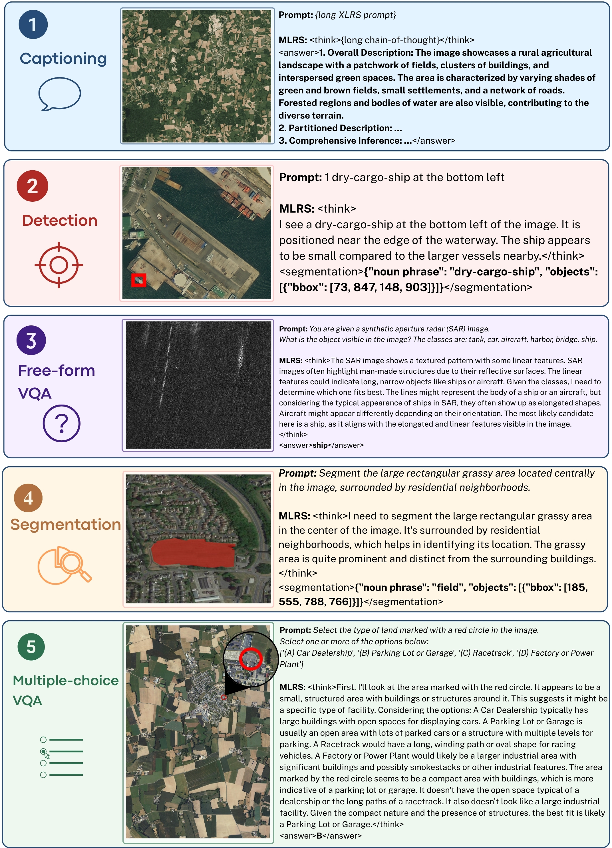
Additional examples of MLRS outputs are provided in Figures 11 and 12.