Do Generative Models Keep Time? A Time-Aware Evaluation of Synthetic Sequential Tabular Data
July 17, 2026
Abstract
Synthetic sequential tabular data are increasingly used for privacy-preserving data sharing, yet a generator can reproduce every marginal and every foreign-key relationship while emitting timestamps that run backwards or repeat, and while sending entities along paths that no real entity followed. Conventional tabular evaluation, which pools records into static distributions, is blind to such failures. We present a taxonomy-guided evaluation protocol for temporal fidelity, in which the applicable measurements are determined by the data rather than fixed in advance. Each dataset is first characterized along four properties — how time is represented, whether observations are regularly sampled, whether trajectories are mutually dependent, and how the schema links entities to their histories — and these properties determine which evaluation dimensions are meaningful. The protocol then measures timestamp validity, cross-sectional structure at aligned time points, within-entity dynamics, and time-varying relational structure, and recasts utility and privacy evaluation over trajectories rather than isolated rows. We apply the protocol to eight generative models across thirteen datasets spanning six domains. Rankings under conventional evaluation disagree substantially with those obtained under temporal evaluation, and the resulting failures are architecture-coherent rather than random. Temporal fidelity must therefore be measured on the time axis itself, rather than inferred from pooled record distributions.
<ccs2012> <concept> <concept_id>10010147.10010178.10010179</concept_id> <concept_desc>Computing methodologies Data generation and augmentation</concept_desc> <concept_significance>500</concept_significance> </concept> <concept> <concept_id>10002950.10003648.10003671</concept_id> <concept_desc>Mathematics of computing Time series analysis</concept_desc> <concept_significance>300</concept_significance> </concept> <concept> <concept_id>10010583.10010786.10010808</concept_id> <concept_desc>Hardware Evaluation</concept_desc> <concept_significance>100</concept_significance> </concept> </ccs2012>
1 Introduction↩︎
The demand for synthetic tabular data has grown rapidly in domains such as finance [1], [2] and healthcare [3], driven by privacy regulations and limited access to sensitive records [4], [5]. Sequential tabular data — in which timestamped records accumulate over time and are grouped by a persistent entity such as a customer, patient, or account [6] — is in fact the dominant data format across many high-stakes domains: transaction logs in finance, visit records in healthcare, usage histories in retail, and sensor streams in industrial systems all share this structure. Despite its ubiquity, the synthesis and evaluation of such data remain critical yet underexplored.
Existing evaluation frameworks overlook the temporal structure of such data. Single-table benchmarks [7], [8] treat records as independent samples, while relational benchmarks [9], [10] evaluate inter-table dependencies but remain agnostic to temporal ordering and population dynamics. Prior work targeting sequential tabular data [6], [11] relies on aggregate-level similarity, leaving cross-sectional dynamics and trajectory-level fidelity unaddressed.

Figure 1 illustrates the consequences of this gap. ClavaDDPM [12], a state-of-the-art relational generative model produces synthetic records that violate chronological order and contain duplicate timestamps, which is incompatible with the constraints of real-world sequential data. However, they are not detected by existing benchmarks: the synthetic data attains near-perfect marginal fidelity on Rossmann (a), as conventional metrics collapse temporal structure into static distributions. The discrepancy emerges under timestamp (b), cross-sectional (c), and trajectory-level (d) inspection where the synthetic population fails to reflect real-world temporal dynamics.
To address this limitation, we introduce Seq2Synth, a unified benchmark for evaluating temporal fidelity in synthetic sequential tabular data. The central claim of this paper is that temporal fidelity cannot be reliably inferred from static or relational fidelity: a generator may match marginal or relational distributions while violating temporal order, distorting population dynamics, corrupting within-entity evolution, or breaking time-varying relational structure. Seq2Synth operationalizes this claim by mapping dataset characteristics to applicable evaluation dimensions and by measuring four complementary forms of temporal fidelity: timestamp validity, cross-sectional fidelity, longitudinal fidelity, and structural consistency. We further extend standard utility and privacy protocols to trajectory-aware settings, so that downstream usefulness and leakage risk are evaluated under sequential dependencies rather than row-level similarity alone.
Contributions. (1) We formulate a taxonomy-guided evaluation protocol for sequential tabular data, where time representation, sampling regularity, cross-trajectory dependence, and schema structure determine which temporal metrics are applicable. (2) We instantiate this protocol in Seq2Synth, covering timestamp, cross-sectional, longitudinal, and structural fidelity, with trajectory-aware utility and privacy extensions. (3) We build a 13-dataset benchmark across six domains and evaluate eight representative generators, showing that static-distribution rankings disagree substantially with temporal-aware rankings and that different architectures fail along distinct temporal dimensions.
2 Related Work↩︎
2.0.0.1 Synthetic Tabular Data Generation
Synthetic data generation has been studied through several approaches. Early relational synthesis methods, such as SDV [13] and RCTGAN [14], relied on hierarchical or conditional generation, while ClavaDDPM [12] incorporated inter-table relationships into diffusion. Recent graph-based methods, including RGCLD [15] and RelDiff [16], use GNNs to model structural dependencies and improve relational consistency. RDB-Diffusion [17] applies structure-aware diffusion to preserve intra-table distributions and inter-table consistency at scale. Meanwhile, the Synthetic Data Vault (SDV) library [18] supports sequential tabular data through CPAR [19], which, along with TabularARGN [20], uses autoregressive modeling in single-table settings. REaLTabFormer [21] (RTF) employs a Seq2Seq-based framework for linear schemas linking parent entities to child trajectory tables. Relevant to our benchmark, TabDiT [11] adopts an autoregressive diffusion Transformer for time-dependent relational data, covering the broadest range of sequential tabular structures among existing methods.
2.0.0.2 Evaluation for Synthetic Data
Various benchmark frameworks have been developed to measure synthetic data quality across modalities. SynthCity [7] and SynthEval [8] provide tools to assess fidelity, utility, and privacy. For relational data, specialized frameworks account for cross-table dependencies and structural consistency: RelBench [10] evaluates utility by transforming tabular records into graph structures and applying graph neural networks to downstream prediction tasks, while SyntheRela [9] measures relational fidelity by aggregating child-table features into parent tables before conducting classifier-based two-sample tests. The SDV library [13] provides evaluation metrics (e.g., SDMetrics) that can capture step-wise distributional similarities for sequential data. Models targeting sequential tabular data evaluate temporal characteristics using model-specific metrics. TabDiT [11] reports MLD-TS and MLE-TS, while TabularARGN [20] employs a coherence metric based on successive time-step pairs. However, these evaluations for sequential tabular data lack a unified and systematic framework for evaluating temporal characteristics across diverse sequential structures, allowing critical failure modes in state-of-the-art models to remain undetected.
3 Seq2Synth Benchmark↩︎
3.0pt max width=
To address the limitations of existing frameworks (See Table ¿tbl:tab:benchmark95comparison?.), evaluates synthetic sequential tabular data through a taxonomy-guided protocol rather than a fixed list of universally applied metrics. Given a real relational dataset \(\mathcal{T}\) and a synthetic counterpart \(\hat{\mathcal{T}}\), the benchmark first identifies the temporal and structural properties of the data, selects the applicable evaluation dimensions, normalizes metric inputs when required, and reports fidelity, utility, and privacy scores under this common protocol.
3.1 Data Model and Taxonomy↩︎
Real-world data such as customer transaction histories and patient visit records share a common structure: timestamped records accumulate over time and are grouped by a persistent entity. We define this class as sequential tabular data. Let \(\mathcal{T} = \{T_1, \ldots, T_D\}\) denote a relational dataset with temporal and referential dependencies, and let \(T \in \mathcal{T}\) be a target table containing \(N\) timestamped records: \[T = \{(x^{key}_i,\, x^{time}_i,\, {\boldsymbol{r}}_i)\}_{i=1}^{N},\] where \(x^{key}_i\) identifies the entity, \(x^{time}_i \in \Omega\) is its timestamp, and \({\boldsymbol{r}}_i = ({\boldsymbol{x}}^{num}_i, {\boldsymbol{x}}^{cat}_i)\) contains numerical and categorical attributes. For each entity \(k\), the rows with \(x^{key}_i=k\), ordered by timestamp, form a trajectory \[T(k) = \{(x^{time}_{k,j},\, {\boldsymbol{r}}_{k,j})\}_{j=1}^{L_k}, \qquad x^{time}_{k,1} \leq \cdots \leq x^{time}_{k,L_k}.\]
3.1.0.1 Taxonomy
Seq2Synth classifies each dataset along four axes that determine which metrics are meaningful: (1) time representation, distinguishing absolute calendar time from relative per-trajectory time; (2) sampling regularity, distinguishing regular grids from irregular event intervals; (3) trajectory dependence, distinguishing population-level dependent trajectories from isolated entities; and (4) schema structure, distinguishing single, linear, multi-child, and multi-parent schemas.2 The taxonomy-to-metric mapping is summarized in Table 7; definitions are in Online Appendix B.
3.2 Benchmark Protocol↩︎
Seq2Synth follows four steps.
3.2.0.1 Step 1: classify the dataset
The dataset is first assigned to the taxonomy above, which determines whether aligned population-level, grid-based, and relational-structure evaluations are applicable.
3.2.0.2 Step 2: select applicable dimensions
The benchmark then selects among four temporal fidelity dimensions. Timestamp and Longitudinal fidelity apply broadly because they evaluate the time axis and within-entity trajectories. Cross-sectional fidelity requires absolute time and dependent trajectories, since it compares population distributions at aligned time points. Structural fidelity is selected according to the schema axis, with additional metrics for multi-child and multi-parent schemas.
3.2.0.3 Step 3: normalize metric inputs
Timestamp metrics are computed on raw generator outputs so that invalid order, duplicate timestamps, out-of-range timestamps, and missing grid points are not hidden by repair. Non-timestamp metrics require well-defined temporal inputs, so Seq2Synth applies a post-processing pipeline before computing cross-sectional, longitudinal, and structural scores: records are sorted, timestamps are aligned when a grid is defined, out-of-range records are trimmed, duplicate entity–timestamp pairs are resolved, and regular-series gaps are imputed. We use the sparse variant as the default for cross-sectional and structural metrics, because leaving missing grid points as NaN exposes temporal coverage failures; longitudinal trajectory metrics use the interpolation-fill variant when complete trajectories are required. Full pipeline details and imputation ablations are in Online Appendix C.
3.2.0.4 Step 4: report dimension-level scores
Each metric produces a score in a common orientation, where higher is better except for reported distances. Scores are aggregated within each dimension over metrics applicable to each dataset. This design prevents inapplicable temporal assumptions from being imposed on datasets with different time representations, sampling patterns, or schema structures.
3.3 Temporal Fidelity Dimensions↩︎
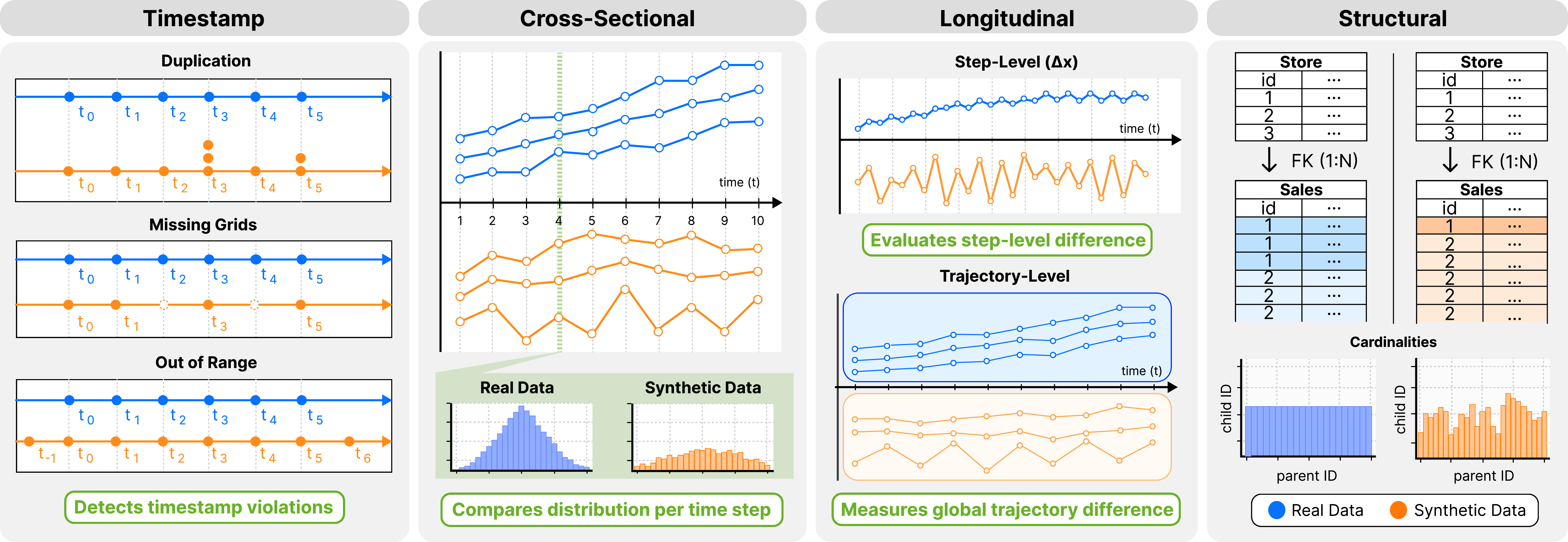
Figure 2 summarizes the four fidelity dimensions.
3.3.0.1 Timestamp fidelity
Timestamp fidelity evaluates the generated time axis independently of feature values. It checks temporal validity through Temporal Order Consistency, , and Temporal Range Compliance; sampling behavior through
Regularity Consistency and Grid Completeness for regular series or Time Interval Distribution Similarity for irregular series; and trajectory span through Trajectory Duration Similarity. These metrics are
computed before post-processing. Full definitions are provided in Appendix 7.2.
3.3.0.2 Cross-sectional fidelity
Cross-sectional fidelity evaluates whether feature distributions are preserved at aligned time points rather than only after pooling all records. It applies when the dataset uses absolute time and contains dependent trajectories. We partition the
temporal domain into intervals and compute distributional similarity within each interval. The instantiated metrics cover numerical marginals (CS-KSComplement), categorical marginals (CS-TVComplement), summary statistics, range
and category coverage, and bivariate dependencies through correlation and contingency similarity. Full definitions are provided in Appendix 7.3.
3.3.0.3 Longitudinal fidelity
Longitudinal fidelity evaluates whether within-entity dynamics are preserved over time. Step-level metrics compare local changes using FirstDiffKSComplement for numerical increments and TransMatrixTVDComplement for categorical
state transitions. Trajectory-level metrics compare longer-range sequential structure using AutoCorrSimilarity, , and TT-Wasserstein Distance where fixed-length trajectories are available. Full definitions are provided in
Appendix 7.4.
3.3.0.4 Structural fidelity
Structural fidelity evaluates whether the temporal relational structure of the data is preserved. applies to all schemas by comparing the distribution of trajectory lengths. Multi-child schemas add and Dynamic K-Hop Correlation Similarity
to test whether child-record counts and cross-table correlations evolve correctly over time. Full definitions are provided in Appendix 7.5.
3.4 Trajectory-aware Utility and Privacy↩︎
3.4.0.1 Utility
Fidelity scores alone do not determine whether synthetic data supports downstream analysis. Seq2Synth adopts the Machine Learning Efficiency protocol, training models on synthetic data and testing them on real data. For sequential tabular data, we
evaluate trajectory-level utility with MLE-TS [11] and additionally report MLE-Temporal, where historical context is included in the
predictive input. The protocol is provided in Appendix [app:utility95metric].
3.4.0.2 Privacy
Standard row-level privacy metrics such as DCR and NNDR ignore whether a synthetic record matches a real record at the same time point or as part of the same trajectory. Seq2Synth therefore adds cross-sectionally restricted
nearest-neighbor metrics, CS-DCR and CS-NNDR, and an \(n\)-gram privacy score, \(\texttt{NGP}(n)=1-\texttt{NgramExposure}(n)\), where higher is safer. Together
these metrics distinguish incidental row-level overlap from time-aligned or sequential leakage. Full definitions are provided in Appendix 7.6.
4 Experiments↩︎
4.1 Experimental Setup↩︎
We evaluate eight generative models on 13 sequential tabular datasets spanning six domains, whose temporal and structural characteristics are categorized in Table 1. We use 7 datasets as the core set because each can be synthesized by at least six of the seven broadly applicable baselines, enabling fairer cross-model comparison. Crucially, these taxonomic axes dictate the applicability of our proposed evaluation dimensions (as detailed in Table 7). Detailed row-level statistics and qualitative descriptions for each dataset are deferred to Online Appendix D.3. The evaluated models include: ClavaDDPM [12], RCTGAN [14], RDBDiff [17], REaLTabFormer (RTF) [21], RGCLD [15], RelDiff [16], SDV [13], and TabDiT [11]. All metric inputs follow the protocol in Section 3.2: sd and ts are computed on raw generator outputs, cs and st use the default sparse variant, and lg uses the interpolation-fill variant when complete trajectories are required. See Online Appendix D for implementation details.
4.2 Results↩︎
| Dataset | Domain | ||||
| Rep. | Period. | ||||
| Indep. | |||||
| Struct. | |||||
| Rossmann | Retail | Abs. | Reg. | Dep. | Linear |
| Berka | Finance | Abs. | Irreg. | Dep. | Linear |
| Fannie Mae | Finance | Abs. | Reg. | Dep. | Linear |
| Walmart | Retail | Abs. | Reg. | Dep. | M-Child |
| AirBnB | Retail | Rel. | Irreg. | Dep. | Linear |
| PTB-XL | Health | Rel. | Reg. | Indep. | Linear |
| Freddie Mac | Finance | Abs. | Reg. | Dep. | Linear |
| Citi Bike | Transport | Abs. | Irreg. | Dep. | Single |
| CMAPSS | Industry | Rel. | Reg. | Indep. | Single |
| Coupon | Retail | Abs. | Irreg. | Dep. | M-C&P |
| Google Cluster | IT | Rel. | Both | Indep. | M-Child |
| H&M | Retail | Abs. | Irreg. | Dep. | M-Parent |
| Home Credit | Finance | Rel. | Reg. | Dep. | M-Child |
3.2pt
We organize the results around three empirical findings that follow the benchmark design in Section 3.2. First, static-distribution evaluation is not a reliable proxy for temporal fidelity: model rankings change substantially when timestamp, longitudinal, and structural fidelity are measured directly. Second, the resulting failures are architecture-coherent rather than random: autoregressive models tend to preserve within-trajectory order but struggle with relational cardinality, while joint and relational generators better preserve some schema-level structure but often fail on timestamp validity and trajectory dynamics. Third, temporal evaluation changes how we interpret both privacy and downstream utility. Online Appendix E reports complete sub-metric tables for the seven core datasets; the main text uses Rossmann and Walmart as representative deep dives because they expose the full timestamp/trajectory and multi-child structural failure modes, respectively.
| Dataset | Metric | ClavaDDPM | RCTGAN | RDBDiff | RTF | RGCLD | RelDiff | SDV | TabDiT |
|---|---|---|---|---|---|---|---|---|---|
| Rossmann | sd | 0.850 | 0.810 | \(\underline{0.858}\) | 0.809 | 0.821 | 0.799 | 0.734 | \(\mathbf{0.932}\) |
| ts | 0.607 | 0.562 | 0.608 | \(\underline{0.823}\) | 0.598 | 0.602 | 0.565 | \(\mathbf{0.824}\) | |
| cs | \(\underline{0.912}\) | 0.808 | \(\underline{0.912}\) | 0.882 | 0.897 | 0.817 | 0.635 | \(\mathbf{0.965}\) | |
| lg | 0.917 | 0.872 | 0.915 | \(\underline{0.948}\) | 0.902 | 0.882 | 0.789 | \(\mathbf{0.975}\) | |
| st | \(\mathbf{1.000}\) | \(\mathbf{1.000}\) | \(\mathbf{1.000}\) | \(\mathbf{1.000}\) | \(\mathbf{1.000}\) | \(\mathbf{1.000}\) | \(\mathbf{1.000}\) | \(\mathbf{1.000}\) | |
| Berka | sd | 0.948 | 0.865 | \(\mathbf{0.992}\) | \(\underline{0.951}\) | 0.922 | 0.898 | 0.695 | 0.909 |
| ts | 0.594 | 0.620 | 0.759 | \(\mathbf{0.907}\) | 0.731 | 0.603 | 0.535 | \(\underline{0.777}\) | |
| cs | \(\underline{0.691}\) | 0.632 | \(\mathbf{0.829}\) | 0.665 | 0.671 | 0.626 | 0.448 | 0.651 | |
| lg | 0.877 | 0.858 | \(\mathbf{0.949}\) | \(\underline{0.896}\) | 0.885 | 0.868 | 0.686 | 0.890 | |
| st | 0.993 | 0.952 | \(\mathbf{1.000}\) | \(\mathbf{1.000}\) | 0.993 | 0.952 | 0.814 | 0.958 | |
| Fannie Mae | sd | \(\underline{0.900}\) | 0.860 | 0.876 | 0.854 | \(\mathbf{0.906}\) | 0.899 | 0.814 | – |
| ts | 0.567 | 0.550 | \(\underline{0.571}\) | 0.474 | 0.503 | \(\mathbf{0.598}\) | 0.481 | – | |
| cs | \(\mathbf{0.965}\) | 0.852 | 0.870 | 0.777 | \(\underline{0.876}\) | 0.849 | 0.772 | – | |
| lg | 0.820 | 0.787 | 0.781 | 0.804 | \(\underline{0.858}\) | 0.822 | \(\mathbf{0.864}\) | – | |
| st | \(\mathbf{0.998}\) | 0.953 | 0.822 | 0.817 | \(\underline{0.990}\) | 0.750 | 0.848 | – | |
| Walmart | sd | 0.796 | 0.861 | 0.815 | 0.719 | \(\mathbf{0.950}\) | \(\underline{0.898}\) | 0.857 | – |
| ts | \(\mathbf{0.610}\) | 0.526 | \(\underline{0.608}\) | 0.455 | 0.600 | 0.598 | 0.522 | – | |
| cs | 0.867 | 0.785 | \(\mathbf{0.896}\) | 0.605 | \(\underline{0.891}\) | 0.828 | 0.746 | – | |
| lg | \(\mathbf{0.887}\) | 0.844 | 0.868 | 0.690 | \(\underline{0.872}\) | 0.852 | 0.814 | – | |
| st | 0.864 | 0.731 | \(\mathbf{0.887}\) | 0.518 | \(\underline{0.882}\) | 0.804 | 0.786 | – | |
| Airbnb | sd | \(\mathbf{0.967}\) | 0.909 | \(\underline{0.963}\) | 0.879 | 0.925 | 0.937 | 0.711 | 0.923 |
| ts | \(\mathbf{0.875}\) | 0.840 | 0.824 | 0.777 | 0.843 | \(\underline{0.860}\) | 0.811 | \(\underline{0.860}\) | |
| cs | – | – | – | – | – | – | – | – | |
| lg | 0.964 | \(\mathbf{0.970}\) | 0.965 | 0.967 | \(\underline{0.969}\) | \(\underline{0.969}\) | 0.909 | 0.965 | |
| st | 0.987 | 0.924 | \(\mathbf{1.000}\) | 0.631 | 0.981 | \(\mathbf{1.000}\) | 0.938 | 0.912 | |
| PTB-XL | sd | \(\underline{0.886}\) | 0.576 | \(\mathbf{0.896}\) | 0.625 | 0.692 | 0.669 | 0.758 | – |
| ts | 0.594 | 0.330 | 0.577 | \(\mathbf{1.000}\) | 0.534 | 0.591 | \(\underline{0.675}\) | – | |
| cs | – | – | – | – | – | – | – | – | |
| lg | \(\mathbf{0.927}\) | 0.841 | 0.909 | 0.915 | 0.906 | \(\underline{0.922}\) | 0.920 | – | |
| st | \(\mathbf{1.000}\) | \(\mathbf{1.000}\) | \(\mathbf{1.000}\) | \(0.999\) | \(\mathbf{1.000}\) | \(\mathbf{1.000}\) | \(\mathbf{1.000}\) | – | |
| Freddie Mac | sd | 0.944 | 0.882 | \(\mathbf{0.986}\) | 0.853 | \(\underline{0.975}\) | 0.920 | 0.810 | – |
| ts | 0.713 | 0.688 | 0.660 | 0.581 | 0.736 | \(\mathbf{0.752}\) | \(\underline{0.747}\) | – | |
| cs | 0.924 | 0.843 | \(\mathbf{0.982}\) | 0.777 | \(\underline{0.930}\) | 0.847 | 0.740 | – | |
| lg | 0.842 | 0.797 | \(\mathbf{0.915}\) | 0.784 | \(\underline{0.875}\) | 0.841 | 0.780 | – | |
| st | 0.995 | 0.972 | \(\mathbf{1.000}\) | 0.695 | 0.993 | \(\mathbf{1.000}\) | 0.965 | – |
2.6pt
4.2.0.1 Finding 1: Static-distribution rankings do not summarize temporal fidelity.
Table 2 reports per-dataset fidelity scores across seven core datasets under five evaluation dimensions: the static-distribution baseline (sd) used in prior benchmarks [7], [9], timestamp validity (ts), cross-sectional distributional evolution (cs), longitudinal trajectory dynamics (lg), and structural consistency (st). The results show that fidelity is strongly dimension-dependent: models with high sd scores do not consistently dominate the temporal-aware dimensions, and the best-performing model often changes across ts, lg, and st. Based on this observation, we analyze rank disagreement between static-distribution and temporal-aware evaluation.
| Dataset | sd vs ts | sd vs cs | sd vs lg | sd vs st | ||||
|---|---|---|---|---|---|---|---|---|
| 2-3 (lr)4-5 (lr)6-7 (lr)8-9 | \(\rho\) | Inv. | \(\rho\) | Inv. | \(\rho\) | Inv. | \(\rho\) | Inv. |
| Airbnb | \(0.714\) | \(0.21\) | – | – | \(-0.071\) | \(0.57\) | \(0.755\) | \(0.22\) |
| Berka | \(0.595\) | \(0.29\) | \(0.905\) | \(0.11\) | \(0.905\) | \(0.11\) | \(0.497\) | \(0.28\) |
| Fannie Mae | \(0.500\) | \(0.33\) | \(0.857\) | \(0.14\) | \(0.071\) | \(0.48\) | \(0.429\) | \(0.38\) |
| Freddie Mac | \(-0.107\) | \(0.52\) | \(1.000\) | \(0.00\) | \(1.000\) | \(0.00\) | \(0.775\) | \(0.20\) |
| PTB-XL | \(0.143\) | \(0.48\) | – | – | \(0.393\) | \(0.33\) | \(0.408\) | \(0.17\) |
| Rossmann | \(0.571\) | \(0.25\) | \(0.929\) | \(0.07\) | \(0.690\) | \(0.21\) | – | – |
| Walmart | \(0.107\) | \(0.43\) | \(0.321\) | \(0.33\) | \(0.250\) | \(0.38\) | \(0.286\) | \(0.38\) |
| Mean (per-ds) | \(0.360\) | \(0.36\) | \(0.802\) | \(0.13\) | \(0.463\) | \(0.30\) | \(0.525\) | \(0.27\) |
| Pooled | \(0.403\) | – | \(0.819\) | – | \(0.477\) | – | \(0.497\) | – |
2.4pt
Table 3 shows that sd-based evaluation is a poor proxy for temporal fidelity. Across the seven core datasets, the rankings induced by timestamp, longitudinal, and structural fidelity diverge substantially from the sd-based ranking, with mean Spearman correlations of \(0.36\), \(0.46\), and \(0.53\), respectively. The corresponding inversion rates are also high: \(36\%\), \(30\%\), and \(27\%\) of model pairs reverse their ordering relative to sd. Thus, models that appear competitive under static-distribution evaluation may fail to preserve temporal validity, trajectory dynamics, or structural consistency.
Cross-sectional fidelity is the only temporal-aware dimension that remains closely aligned with sd evaluation, with pooled \(\rho=0.82\) and a mean inversion rate of \(13\%\). This is because the cross-sectional dimension evaluates distributional similarity within individual time slices and then aggregates the slice-wise scores over time. As a result, it retains much of the ranking signal captured by static-distribution evaluation, but with a finer temporal resolution. This suggests that cross-sectional fidelity contributes less by producing a different global model ranking and more by diagnosing whether distributional fidelity is stable across time. A model can achieve a strong pooled sd score while still failing on specific time slices, and the cross-sectional dimension is designed to expose such temporally localized distributional failures. These rank disagreements establish the main empirical premise of Seq2Synth: temporal fidelity cannot be reduced to a single architecture-independent notion of quality. The next analysis explains why the rankings diverge by decomposing model behavior into timestamp, cross-sectional, longitudinal, and structural failure modes.
4.2.0.2 Finding 2: Temporal sub-metrics expose model-specific failures.
| \(0.507\) | \(0.629\) | \(0.462\) | \(0.402\) | \(0.644\) | |
| \(\mathbf{0.512}\) | \(0.594\) | \(0.287\) | \(0.372\) | \(0.611\) | |
| \(\underline{0.510}\) | \(0.628\) | \(0.466\) | \(0.402\) | \(0.644\) | |
| \(0.001\) | \(\mathbf{0.999}\) | \(\underline{0.942}\) | \(\mathbf{0.997}\) | \(\mathbf{0.999}\) | |
| \(0.507\) | \(0.619\) | \(0.435\) | \(0.392\) | \(0.636\) | |
| \(0.509\) | \(0.616\) | \(0.507\) | \(0.369\) | \(0.618\) | |
| \(0.508\) | \(0.594\) | \(0.350\) | \(0.364\) | \(0.596\) | |
| \(0.023\) | \(\underline{0.978}\) | \(\mathbf{1.000}\) | \(\underline{0.959}\) | \(\underline{0.983}\) |
2.8pt
Timestamp. Timestamps encode trajectory-level structure that ordinary marginal fidelity metrics cannot capture. We first examine whether the eight models generate valid timestamp structure on Rossmann, including uniqueness, regular spacing, grid coverage, and trajectory duration. Table 4 reports timestamp sub-metric scores on Rossmann, a regular time-series dataset. The columns denote , , , , and , respectively, all computed before post-processing. Together, these metrics distinguish misordered records, duplicate timestamps, unrealistic durations, irregular intervals, and incomplete observation grids. The results reveal a clear architectural divide. For the timestamp properties that remain meaningful after user-side reordering—uniqueness, duration, regularity, and grid coverage—RTF and TabDiT occupy the top two ranks with scores above \(0.94\), while the six joint-generation models remain substantially lower. This gap reflects the advantage of autoregressive decoding: by emitting events sequentially and conditioning each timestamp on previously generated ones, RTF and TabDiT better preserve uniqueness, regular spacing, duration, and grid coverage. In contrast, joint-generation models sample timestamps in parallel with other features, leading to duplicate timestamps, mismatched durations, irregular intervals, and missing grid slots. These errors are invisible to sd and cannot be resolved by simple reordering.
| Model | -KSComp | -TVComp | -StatSim | -CatCov | -ContSim |
|---|---|---|---|---|---|
| ClavaDDPM | \(\underline{0.951}\) | \(0.912\) | \(0.775\) | \(\underline{0.969}\) | \(0.828\) |
| RCTGAN | \(0.874\) | \(0.688\) | \(0.723\) | \(\mathbf{0.972}\) | \(0.505\) |
| RDBDiff | \(0.948\) | \(\underline{0.913}\) | \(0.774\) | \(\underline{0.969}\) | \(\underline{0.830}\) |
| RTF | \(0.904\) | \(0.828\) | \(\underline{0.875}\) | \(0.910\) | \(0.702\) |
| RGCLD | \(0.940\) | \(0.892\) | \(0.765\) | \(0.935\) | \(0.806\) |
| RelDiff | \(0.881\) | \(0.738\) | \(0.681\) | \(\mathbf{0.972}\) | \(0.563\) |
| SDV | \(0.562\) | \(0.496\) | \(0.727\) | \(0.734\) | \(0.263\) |
| TabDiT | \(\mathbf{0.996}\) | \(\mathbf{0.947}\) | \(\mathbf{0.947}\) | \(\mathbf{0.972}\) | \(\mathbf{0.896}\) |
3.0pt
Cross-sectional dimension. Table 5 shows the cross-sectional sub-metric profiles on Rossmann. The displayed columns correspond to CS-KSComplement, CS-TVComplement, ,
CS-CategoryCoverage, and . TabDiT has the strongest cross-sectional profile, ranking best on most sub-metrics. Some models show asymmetric behavior that an aggregate score can obscure: RCTGAN and RelDiff achieve high category coverage but much
lower contingency similarity, indicating that they recover per-slice category values without preserving their joint combinations. SDV shows the weakest profile, especially on contingency similarity. These results suggest that cross-sectional fidelity
requires more than matching marginal distributions or category coverage within each time slice; it also requires preserving relationships among features.
![Figure 3: Longitudinal sub-metric profiles on Rossmann under the interpolation-fill variant. All scores lie in [0,1], with higher values indicating better longitudinal fidelity.](/article/2607.15606/figs/rossmann_lg_heatmap.png "fig:")
Longitudinal dimension. Figure 3 reports the longitudinal sub-metric profiles on Rossmann. The columns correspond to , , and . TabDiT exhibits the strongest longitudinal profile, leading on the first-difference and transition-matrix metrics, while RTF also performs strongly on the order-sensitive metrics. This pattern is consistent with the within-trajectory advantage of autoregressive decoding observed in the timestamp analysis. The differences across sub-metrics show that longitudinal fidelity is not a single property. ClavaDDPM and SDV preserve autocorrelation relatively well, but are weaker on local changes and transition patterns, while RTF shows the opposite behavior. Thus, local changes, transitions, and temporal dependence should be evaluated separately because they capture different aspects of within-entity dynamics.
![Figure 4: Structural fidelity sub-metrics on Walmart. All scores are normalized in [0,1], with higher values indicating better structural fidelity.](/article/2607.15606/figs/st_walmart_2.png "fig:")
Temporal relational structure. Figure 4 describes structural sub-metric profiles on Walmart, the only core dataset with applicable st sub-metric data. The 3 sub-metrics
evaluate Sequence Length Similarity, Temporal Cardinality Shape Similarity, and Dynamic K-Hop Correlation Similarity. The first 2 sub-metrics are computed from raw generator output, whereas uses the sparse variant.
RTF reveals a limitation of autoregressive sequence generation in relational settings. Although it performs strongly on timestamp and longitudinal dimensions, its low structural fidelity is mainly driven by failures in and , indicating that it does not
reliably control the number of child records per parent or their temporal cardinality patterns. By contrast, relational diffusion models such as RDBDiff and ClavaDDPM improve substantially under st, despite weaker sd rankings, because their joint generation under the relational schema better preserves sequence length and cross-table correlation structure across parent entities.
4.2.0.3 Finding 3: Temporal evaluation provides a complementary lens beyond static privacy and utility metrics.
| Model | Row-level | Cross-sectional | \(n\)-gram Privacy | |||
|---|---|---|---|---|---|---|
| 2-3 (lr)4-5 (lr)6-7 | DCR | NNDR | CS-DCR | CS-NNDR | NGP(1) | NGP(3) |
| ClavaDDPM | \(8.06\) | \(0.707\) | \(49.46\) | \(0.653\) | \(0.002\) | \(0.912\) |
| RCTGAN | \(9.22\) | \(0.709\) | \(73.48\) | \(0.695\) | \(0.074\) | \(\underline{0.998}\) |
| RDBDiff | \(6.08\) | \(0.662\) | \(16.24\) | \(0.489\) | \(0.000\) | \(0.833\) |
| RTF | \(9.06\) | \(\underline{0.721}\) | \(64.80\) | \(\underline{0.742}\) | \(0.028\) | \(0.180\) |
| RGCLD | \(8.06\) | \(0.707\) | \(54.72\) | \(0.697\) | \(0.014\) | \(0.907\) |
| RelDiff | \(\mathbf{12.04}\) | \(0.703\) | \(\mathbf{96.72}\) | \(0.693\) | \(\underline{0.209}\) | \(\underline{0.998}\) |
| SDV | \(\underline{9.85}\) | \(0.707\) | \(\underline{86.76}\) | \(0.661\) | \(\mathbf{0.221}\) | \(\mathbf{0.999}\) |
| TabDiT | \(11.00\) | \(\mathbf{0.766}\) | \(62.84\) | \(\mathbf{0.753}\) | \(0.008\) | \(0.267\) |
2.6pt
Privacy. Standard DCR, NNDR, and single-row exposure treat synthetic and real records as exchangeable across time. Two practical concerns motivate temporal restrictions. First, two records sharing values at
unrelated timestamps are often not a re-identification risk: bounded row vocabularies make such incidental overlap common (for instance, 20% of session records in Airbnb share identical row-level values with at least one other record), and the
concern is whether identifying values concentrate at the same time slice as a real record. Second, plausible synthetic rows can still reproduce consecutive sub-sequences of a real trajectory, which row-level overlap counts cannot detect.
We therefore compare row-level metrics with CS-DCR, CS-NNDR, and \(n\)-gram privacy (\(\texttt{NGP}(n)=1-\texttt{NgramExposure}(n)\)) on Rossmann.
Under the higher is safer convention, Table 6 shows that row-level privacy metrics can misrepresent temporal privacy risk.
3pt max width=
Time-agnostic nearest-neighbor metrics such as DCR and NNDR ignore whether matched synthetic and real rows belong to the same time slice. In low-cardinality sequential data, this can count incidental cross-time matches as
privacy risk; the larger CS-DCR values indicate that row-level nearest neighbors come from unrelated timestamps. Conversely, single-row exposure can miss sequential leakage: NGP\(^{(1)}\) does not
detect copied consecutive sub-sequences. RTF and TabDiT illustrate this failure, appearing safe under row-level metrics but becoming the riskiest models under NGP\(^{(3)}\). Thus, the autoregressive mechanism
that improves within-trajectory fidelity can increase trajectory-level privacy risk. Results on the remaining 6 datasets are reported in Online Appendix E.5.
Utility. Table ¿tbl:tab:rho95corr95mle95ts95temporal? reports correlation results on the four datasets shared by MLE-TS and MLE-Temporal. The results show that sd-based evaluation does not fully explain downstream temporal utility. Under MLE-TS, the average longitudinal correlation (\(\rho_{\mathrm{long}}=0.399\)) is higher than the sd correlation (\(\rho_{\mathrm{SD}}=0.173\)). The pattern becomes stronger under MLE-Temporal, where longitudinal fidelity is more aligned with utility than sd (\(\rho_{\mathrm{long}}=0.682\) vs.\(\rho_{\mathrm{SD}}=0.402\)). This increase suggests that when the downstream protocol explicitly preserves chronological
structure, utility depends more on whether synthetic data captures within-trajectory dynamics than on whether it matches static marginal distributions alone. This gap widens from MLE-TS to MLE-Temporal, suggesting that temporal
fidelity becomes increasingly task-relevant as the downstream protocol uses more historical context. Full results are available in Online Appendices E.2 and E.3.
5 Discussion↩︎
5.0.0.1 Implications for benchmark use.
The results provide empirical evidence that Seq2Synth should be used as a diagnostic protocol rather than as a single leaderboard score. Static-distribution fidelity remains useful for checking pooled record-level plausibility, but it is insufficient for model selection when the deployment depends on temporal behavior. The taxonomy-to-metric mapping is therefore essential: timestamp and longitudinal metrics test whether individual trajectories are valid, cross-sectional metrics test whether population structure evolves correctly over absolute time, and structural metrics test whether relational cardinalities and cross-table dependencies are preserved. These dimensions should be interpreted jointly, because a model can be strong along one temporal axis and fail along another. The same principle applies to privacy and utility: row-level privacy and static downstream performance should be complemented by trajectory-aware views when sequential leakage or temporal prediction is the relevant risk.
5.0.0.2 Implications for generator design.
The failure modes identified by Seq2Synth point to three concrete design requirements for future sequential-tabular generators. First, timestamps should be modeled as ordered objects rather than as ordinary continuous attributes; otherwise, a model can match timestamp marginals while producing invalid chronological structure. Second, autoregressive generators need explicit absolute-time anchoring, such as calendar embeddings, anchor tokens, or auxiliary timestamp losses, so that token position is not confused with calendar time. Third, sequence length and relational cardinality should be conditioned on directly rather than left to emerge implicitly, especially in multi-table schemas where parent–child counts evolve over time. These changes do not require a new model family: they can be incorporated into existing diffusion, autoregressive, or relational generators through constrained decoding, auxiliary objectives, or conditioning inputs.
6 Conclusion↩︎
We presented Seq2Synth, a taxonomy-guided benchmark for evaluating synthetic sequential tabular data. Rather than treating all datasets with a fixed metric suite, Seq2Synth maps time representation, sampling regularity, trajectory dependence, and schema structure to applicable temporal fidelity dimensions: timestamp, cross-sectional, longitudinal, and structural fidelity. Across a 13-dataset benchmark and eight generators, our experiments show that static-distribution fidelity is not a reliable proxy for temporal fidelity: models that appear strong under conventional evaluation can still produce invalid timestamps, distorted trajectories, or inconsistent temporal relational structure. The trajectory-aware utility and privacy analyses further show that temporal evaluation changes how model quality and leakage risk should be interpreted. These findings support a simple principle: synthetic sequential tabular data should be evaluated as temporally ordered trajectories and relational processes, not as pooled rows.
| Perspective | Metric Name | Scope | Applicable Features | Time Repr. | Periodicity | Traj. Indep. | Data Str. |
|---|---|---|---|---|---|---|---|
| TimeIntervalDistributionSimilarity | U | \(x^{time}\) | Both | Irregular | Both | All | |
| RegularityConsistency | U | \(x^{time}\) | Both | Both | Both | All | |
| TemporalRangeCompliance | U | \(x^{time}\) | Both | Both | Both | All | |
| GridCompleteness | U | \(x^{time}\) | Both | Regular | Both | All | |
| TemporalOrderConsistency | U | \(x^{time}\) | Both | Both | Both | All | |
| TimestampUniqueness | U | \(x^{time}\) | Both | Both | Both | All | |
| TrajectoryDurationSimilarity | U | \(x^{time}\) | Both | Both | Both | All | |
| CS-KSComplement | U | Each \(x^{num}\) | Abs. | Both | Dep. | All\(^*\) | |
| CS-StatisticSimilarity | U | Each \(x^{num}\) | Abs. | Both | Dep. | All\(^*\) | |
| CS-RangeCoverage | U | Each \(x^{num}\) | Abs. | Both | Dep. | All\(^*\) | |
| CS-TVComplement | U | Each \(x^{cat}\) | Abs. | Both | Dep. | All\(^*\) | |
| CS-CategoryCoverage | U | Each \(x^{cat}\) | Abs. | Both | Dep. | All\(^*\) | |
| CS-CorrelationSimilarity | B | Each \((x^{num}_a, x^{num}_b)\) pair | Abs. | Both | Dep. | All\(^*\) | |
| CS-ContingencySimilarity | B | Each \((x^{cat}_a, x^{cat}_b)\) pair | Abs. | Both | Dep. | All\(^*\) | |
| FirstDifferenceKSComplement | U | Each \(x^{num}\) | Both | Regular | Both | All | |
| TransitionMatrixTVDComplement | U | Each \(x^{cat}\) | Both | Regular | Both | All | |
| AutoCorrelationSimilarity | U | Each \(x^{num}\) | Both\(^\dagger\) | Regular | Both\(^\dagger\) | All | |
| TT-WassersteinDistance ([22]) | M | All \(x^{num}\) jointly | Both | Regular | Both | All | |
| MLD-TS ([11]) | M | All features at time \(t\) | Both | Both | Both | All | |
| SequenceLengthSimilarity | U | trajectory length \(L_k\) | Both | Both | Both | All | |
| TemporalCardinalityShapeSimilarity | U | Each parent–child relation | Abs. | Both | Both | M-Child | |
| DynamicKHopCorrelationSimilarity | B | Cross-table \((x_a, x_b)\) pair | Abs. | Regular | Dep. | M-Child | |
| CS-DCR | M | All features at time \(t\) | Abs. | Both | Dep. | All | |
| CS-NNDR | M | All features at time \(t\) | Abs. | Both | Dep. | All | |
| n-gramPrivacy | M | All features at time \(t\) | Both | Both | Both | All | |
| MLE-TS | M | All features at time \(t\) | Abs. | Both | Both | All | |
| MLE-Temporal | M | All features at time \(t\) | Abs. | Regular | Both | All |
7 Evaluation Metrics↩︎
This appendix gives the operational definition of every metric used in the main paper. All metrics produce a scalar in \([0,1]\) unless noted otherwise; \(1\) denotes perfect fidelity. Notation follows Section 3.1: \(T\) and \(\hat{T}\) are the real and synthetic tables, \(x^{time}_{k,j}\) is the timestamp of the \(j\)-th record of trajectory \(k\), \(\Delta t_{k,j}=x^{time}_{k,j}-x^{time}_{k,j-1}\), \(L_k\) is trajectory length, and \(K\) is the number of trajectories.
7.1 Feature Scope and Aggregation↩︎
Each metric operates at one of three scopes: univariate (per feature column \(f\)), bivariate (per feature pair \((f_1,f_2)\)), or multivariate (joint feature vector / trajectory embedding). For univariate and bivariate metrics, the per-feature (or per-pair) score is averaged uniformly across the applicable set \(\mathcal{F}\) (or \(\mathcal{P}\)): Applicable features per metric (numerical only, categorical only, both) are listed in the online appendix’s metric-applicability table.
7.2 Timestamp Metrics↩︎
All timestamp metrics are computed on the raw synthetic output before sorting, deduplication, boundary trimming, or imputation, so generator-level timestamp failures are not hidden by post-processing.
TemporalOrderConsistency (TempOrderConsist; all series) measures the fraction of consecutive timestamp pairs that are non-decreasing: \[1 - \frac{\sum_k
\sum_{j=2}^{L_k} \mathbb{I}(\Delta t_{\mathrm{synth},k,j} < 0)}{\sum_k (L_k - 1)}. \label{eq:chrono}\tag{1}\]
TimestampUniqueness (TimestampUnique; all series) measures the fraction of consecutive intervals that are strictly positive, detecting duplicate timestamps before deduplication:
\[1 - \frac{\sum_k \sum_{j=2}^{L_k} \mathbb{I}(\Delta t_{\mathrm{synth},k,j} = 0)}{\sum_k (L_k - 1)}. \label{eq:uniqueness}\tag{2}\]
TemporalRangeCompliance (TempRangeComp; all series) measures the fraction of synthetic records within the valid real temporal domain \(\Omega_{\mathrm{real}}\); for relative time, the first
timestamp must also be anchored at zero: \[1 - \frac{1}{N_{\mathrm{synth}}}\sum_k \sum_j V_{k,j}, \label{eq:boundary}\tag{3}\] where \(V_{k,j}\) is the per-record violation indicator.
RegularityConsistency (RegularityConsist; regular series only) measures the fraction of synthetic intervals matching the canonical interval \(c\) within tolerance \(\epsilon=0.01c\): \[1 - \frac{\sum_k \sum_{j=2}^{L_k} \mathbb{I}(|\Delta t_{\mathrm{synth},k,j} - c| > \epsilon)}{\sum_k (L_k - 1)}.
\label{eq:regularity}\tag{4}\]
GridCompleteness (GridCompleteness; regular series only) compares real and synthetic canonical grid-point multiplicities, capping synthetic credit at the real multiplicity: \[\frac{\sum_g
\min(M_{\mathrm{real}}(g), M_{\mathrm{synth}}(g))}{\sum_g M_{\mathrm{real}}(g)}.\]
TimeIntervalDistributionSimilarity (TimeIntervalDistrSim; irregular series only) compares pooled real and synthetic inter-arrival distributions using the KS complement: \[1 - \sup_{\Delta t} \bigl|F_{\mathrm{real}}(\Delta t) - F_{\mathrm{synth}}(\Delta t)\bigr|. \label{eq:timedist}\tag{5}\]
TrajectoryDurationSimilarity (TrajDurationSim; all series) compares real and synthetic trajectory-duration distributions using the KS complement, with \(D_k=x^{time}_{k,L_k}-x^{time}_{k,1}\): \[1 - \sup_D \bigl|F_{\mathrm{real}}(D) - F_{\mathrm{synth}}(D)\bigr|. \label{eq:duration}\tag{6}\]
7.3 Cross-Sectional Metrics↩︎
Cross-sectional metrics compare real and synthetic feature distributions within aligned temporal partitions. They apply to datasets with Absolute Time and Dependent Trajectories. Let \(\Omega=\bigsqcup_{l=1}^{B}\Omega_l\) be a partition of the temporal domain, and let \(T\vert_l\) and \(\hat{T}\vert_l\) be records whose timestamps fall in \(\Omega_l\). Any base measure \(\mu\) is lifted to a cross-sectional metric as \[\label{eq:cs95general} \mu_{CS}(T,\hat{T}) = \frac{1}{B}\sum_{l=1}^{B} \mu(T\vert_l,\hat{T}\vert_l).\tag{7}\] For feature \(f\), \(T_l^{(f)}\) and \(\hat{T}_l^{(f)}\) denote values in partition \(\Omega_l\); \(F_{T_l}^{(f)}\) is the numerical CDF and \(P_{T_l}^{(f)}\) the categorical distribution.
CS-KSComplement compares numerical distribution shapes within each time partition: \[\mu^{KS}(T\vert_l,\hat{T}\vert_l) = 1 - \sup_x \left|F_{T_l}^{(f)}(x) - F_{\hat{T}_l}^{(f)}(x)\right|.\]
CS-StatisticSimilarity compares time-local summary statistics \(S\in\{\mathrm{mean},\mathrm{median},\mathrm{std}\}\): \[\mu^{Stat}_{S}(T\vert_l,\hat{T}\vert_l) = 1 - \frac{ \left|S(T_l^{(f)}) - S(\hat{T}_l^{(f)})\right| }{ \max_{l'} S(T_{l'}^{(f)}) - \min_{l'} S(T_{l'}^{(f)}) + \epsilon },\] with the reported score averaged over the three statistics and clipped to \([0,1]\).
CS-RangeCoverage measures whether synthetic numerical values remain inside the real range at each time partition: \[\mu^{Range}(T\vert_l,\hat{T}\vert_l) = \frac{1}{|\hat{T}_l^{(f)}|} \sum_{x\in\hat{T}_l^{(f)}} \mathbb{I}\!\left[ x \in \left[\min T_l^{(f)}, \max T_l^{(f)}\right] \right].\]
CS-TVComplement compares categorical distributions using the total variation complement: \[\mu^{TV}(T\vert_l,\hat{T}\vert_l) = 1 - \frac{1}{2} \sum_{c} \left|P_{T_l}^{(f)}(c) - P_{\hat{T}_l}^{(f)}(c)\right|.\]
CS-CategoryCoverage measures whether real categories at a time partition also appear in synthetic data: \[\mu^{CatCov}(T\vert_l,\hat{T}\vert_l) = \frac{ |C_{T_l}^{(f)} \cap C_{\hat{T}_l}^{(f)}| }{ |C_{T_l}^{(f)}| },\] where empty real partitions are excluded from the average.
CS-CorrelationSimilarity compares numerical pairwise correlations within each time partition: \[\mu^{Corr}(T\vert_l,\hat{T}\vert_l) = 1 - \frac{ |\rho_{T_l}(f_1,f_2) - \rho_{\hat{T}_l}(f_1,f_2)| }{2}.\]
CS-ContingencySimilarity compares categorical co-occurrence patterns using the TV complement over joint category frequencies: \[\mu^{Cont}(T\vert_l,\hat{T}\vert_l) = 1 - \frac{1}{2} \sum_{a}\sum_{b} \left|
P_{T_l}^{(f_1,f_2)}(a,b) - P_{\hat{T}_l}^{(f_1,f_2)}(a,b) \right|.\]
7.4 Longitudinal Metrics↩︎
Longitudinal metrics treat each entity as an ordered trajectory. Step-level metrics compare consecutive changes; trajectory-level metrics compare longer range temporal structure. Except for and raw MLD-TS detection accuracy, larger values
indicate better fidelity.
FirstDifferenceKSComplement (; numerical). Measures whether synthetic local increments match real increments, using pooled first differences \(\Delta x_{k,j}=x_{k,j}-x_{k,j-1}\): \[1 - \sup_{\delta} \left| F^{\Delta}_{\mathrm{real}}(\delta) - F^{\Delta}_{\mathrm{synth}}(\delta) \right|. \label{eq:fd95ks}\tag{8}\] Scores are computed per numerical feature and aggregated as described in Appendix 7.1.
TransitionMatrixTVDComplement (TransMatrixTVDComplement; categorical). For category set \(C\) and valid transition times \(\mathcal{T}\),
\[1-
\frac{1}{2|C||\mathcal{T}|}
\sum_{t\in\mathcal{T}}\sum_{i,j\in C}
\left|P^r_t(j\mid i)-P^s_t(j\mid i)\right|.
\label{eq:transition}\tag{9}\] Here \(P^r_t\) and \(P^s_t\) denote real and synthetic transition probabilities; scores are averaged over categorical features. Scores are
computed per categorical feature and averaged.
AutocorrelationSimilarity (; numerical). Measures whether lag-wise temporal dependence is preserved by comparing autocorrelation profiles up to \(H=\min(L/4,50)\): \[1 - \frac{1}{2H}\sum_{h=1}^{H} \left| \rho^{\mathrm{real}}_h - \rho^{\mathrm{synth}}_h \right|. \label{eq:acf}\tag{10}\] For independent trajectories, autocorrelation is computed per trajectory and averaged; for dependent trajectories with shared absolute time, it is computed on the cross-sectional mean trajectory.
MLD-TS (MLD-TS; multivariate). MLD-TS evaluates whether real and synthetic trajectories are distinguishable by a supervised classifier. Each trajectory is embedded as \(z_k=\psi(T(k))\),
labeled by source, and classified by \(h\); raw MLD-TS is detection accuracy: \[\frac{1}{|\mathcal{D}_{\mathrm{test}}|}
\sum_{(z,y)\in\mathcal{D}_{\mathrm{test}}} \mathbb{I}\{h(z)=y\}. \label{eq:mld95ts}\tag{11}\] Values near chance indicate low distinguishability, while higher values indicate more detectable temporal mismatch. Classifier settings are provided
in Online Appendix D.6.
TT-WassersteinDistance (TT-WassersteinDistance; multivariate). TT-Wasserstein compares the global distribution of trajectory patterns via spectral embeddings. Each trajectory \(X\in\mathbb{R}^{L_k\times C}\) is z-score normalized, first-differenced, and mapped to Fourier-magnitude features: \[\phi^{(c)}(X) = \bigl|\mathrm{DFT}(z^{(c)}_t - z^{(c)}_{t-1})_{1:F}\bigr|, \qquad
\phi(X)=\mathrm{vec}([\phi^{(1)},\ldots,\phi^{(C)}]).\] With cost \(M_{ij}=\|\phi(X_i^{\mathrm{real}})-\phi(X_j^{\mathrm{synth}})\|^2\), \[D_{\mathrm{TTW}} = \left( \min_{\Gamma\in\Pi(a,b)} \sum_{i,j}\Gamma_{ij}M_{ij} \right)^{1/2}. \label{eq:tt95wasserstein}\tag{12}\] Smaller \(D_{\mathrm{TTW}}\) indicates better
preservation of the trajectory distribution; it is reported as a distance rather than a \([0,1]\) similarity.
7.5 Structural Metrics↩︎
Structural metrics evaluate relational properties of sequential data; larger values indicate better structural fidelity.
SequenceLengthSimilarity (adopted from SDMetrics [18]; all schemas) compares the real and synthetic trajectory-length distributions: \[1 - \sup_{L} \left| F_{\mathrm{real}}(L) - F_{\mathrm{synth}}(L) \right|. \label{eq:seq95len}\tag{13}\]
TemporalCardinalityShapeSimilarity (temporal extension of SyntheRela’s CardinalityShapeSimilarity [9]; multi-child schemas) compares the window-level child-record count distributions for each parent–child relation: \[1 - \sup_{s} \left| F_{\mathrm{real}}(s) - F_{\mathrm{synth}}(s) \right|, \label{eq:cardinality}\tag{14}\] where \(s\) denotes child-record counts within aligned temporal windows.
DynamicKHopCorrelationSimilarity (temporal extension of SyntheRela’s \(k\)-hop correlation similarity [9]; multi-child schemas) compares cross-table correlations over time for variables linked by a \(k\)-hop foreign-key path: \[1 - \frac{1}{|\mathbb{T}_{\mathrm{eval}}|} \sum_{t\in\mathbb{T}_{\mathrm{eval}}} \frac{| \rho_{\mathrm{real}}(t) - \rho_{\mathrm{synth}}(t) |}{2}. \label{eq:khop}\tag{15}\] The score is averaged over applicable \(k\)-hop variable pairs, with \(k=1\) by default.
7.6 Privacy and Utility Metrics↩︎
Privacy metrics evaluate three leakage granularities: row-level proximity (DCR, NNDR), same-time-slice proximity (CS-DCR, CS-NNDR), and sequential-pattern privacy (NGP(n)). Higher values
are safer, except that DCR and CS-DCR are raw distances. Let \(X^{(i)}_{\rm real}\) be the numerical feature vector of real record \(i\).
DCR measures the median nearest-neighbor distance from each real record to the synthetic table: \[\operatorname{Median}_{i} \left( \min_j \left\| X^{(i)}_{\mathrm{real}} - X^{(j)}_{\mathrm{synth}} \right\|_2 \right).\]
NNDR is the median ratio between the first- and second-nearest synthetic neighbors of each real record; higher ratios imply fewer isolated near-matches.
CS-DCR and CS-NNDR restrict the same nearest-neighbor computations to records in the same timestamp or temporal partition: \[\operatorname{Median}_{t\in\mathbb{T}_{\mathrm{eval}}}
\operatorname{Median}_{i:x^{time}_i=t}
\left(
\min_{j:\hat{x}^{time}_j=t}
\left\|
X^{(i)}_{\mathrm{real}} -
X^{(j)}_{\mathrm{synth}}
\right\|_2
\right),\] with CS-NNDR defined analogously using same-time-slice first- and second-nearest neighbors.
\(n\)-gramPrivacy NGP(n) measures whether discretized synthetic trajectory fragments reproduce real length-\(n\) token subsequences:
\[\mathrm{NgramExposure}(n) = \frac{1}{|\hat{\mathcal{K}}|} \sum_{k\in\hat{\mathcal{K}}} \frac{1}{|G_k^{(n)}|} \sum_{g \in G_k^{(n)}} \mathbb{I}\!\left(g \in
\mathcal{G}_{\mathrm{real}}^{(n)}\right), \label{eq:ngram95exposure}\tag{16}\] where \(G_k^{(n)}\) is the set of synthetic length-\(n\) token subsequences and \(\mathcal{G}_{\mathrm{real}}^{(n)}\) is the real subsequence set. We define \[\mathrm{NGP}(n) = 1 - \mathrm{NgramExposure}(n), \label{eq:ngp}\tag{17}\]
with NGP(1) and NGP(3) distinguishing single-row from longer within-trajectory sequential-pattern reproduction.
MLE-TS (MLE-TS) MLE-TS uses the same protocol as MLD-TS, but trains a downstream predictor instead of a detector. For each trajectory \(T^a(k)\), \(a\in\{\mathrm{real,synth}\}\), we compute \(z_k^a=\psi(T^a(k))\) and pair it with label \(y_k\). A predictor \(f_g\) trained on synthetic pairs is evaluated on held-out real trajectories by \[\mathrm{MLE\text{-}TS}(g)
=
\mathrm{AUC}\bigl(\{f_g(z_k^{\mathrm{real}})\},\{y_k^{\mathrm{real}}\}\bigr).\]
MLE-Temporal (MLE-Temporal) MLE-Temporal adapts the same train-on-synthetic, test-on-real protocol to record-level prediction under a chronological split. For each trajectory \(T^a(k)\),
\(a\in\{\mathrm{real,synth}\}\), and prediction time \(t\), we compute \(z_{k,t}^a=\psi(T^a(k)_{\le t})\) from the history observed up to \(t\) and pair it with label \(y_{k,t}\). A predictor \(f_g\) trained on synthetic temporal pairs is evaluated on held-out real pairs from later timestamps by
\[\mathrm{MLE\text{-}Temporal}(g)
=
\mathcal{M}\!\left(
\{f_g(z_{k,t}^{\mathrm{real}})\}_{(k,t)\in\mathcal{D}_{\mathrm{test}}^{\mathrm{real}}},
\{y_{k,t}^{\mathrm{real}}\}_{(k,t)\in\mathcal{D}_{\mathrm{test}}^{\mathrm{real}}}
\right),\] where \(\mathcal{M}\) is AUC for classification and \(R^2\) for regression. It measures whether synthetic data preserve task-relevant historical dynamics for time-ordered
record-level prediction.
8 Taxonomy: Formal Definitions↩︎
Temporal Characteristics. Observations with Absolute Time operate on a globally shared calendar domain \(\mathbb{T}_{global}\), so simultaneous events across trajectories share the same temporal reference: \(x^{time}_{k,j} \in \mathbb{T}_{global}\). In Relative Time, each trajectory operates on its own lifecycle timeline, with the first observation normalized to zero: \(x^{time}_{k,1} = 0\;\forall k\). A Regular series has a fixed inter-arrival interval \(c\): \(\Delta t_{k,j} = c\;\forall k, j\). An Irregular series has stochastic inter-arrival times drawn from a distribution \(P(\Delta t)\): \(\Delta t_{k,j} \sim P(\Delta t)\).
Trajectory Dynamics. Independent trajectories represent entirely isolated entities; the trajectory of one carries no information about another: \(P(T(k), T(k')) = P(T(k))\,P(T(k'))\) for any \(k \neq k'\). Dependent trajectories share macro-level dynamics, so their trajectories are statistically correlated: \(\exists\, k \neq k'\) s.t.\(P(T(k), T(k')) \neq P(T(k))\,P(T(k'))\). Evaluating trajectory dependencies requires Absolute Time, as a globally shared axis is a prerequisite for aligning observations across trajectories.
Structural Complexity. We characterize relational schemas by the number of 1:N foreign-key relationships each row participates in. Given parent table \(T_p\), child table \(T_c\), and FK map \(f_{FK}: T_c \to T_p\), the child set of a parent row is \(\mathcal{C}(\mathbf{r}_p) = \{\mathbf{r}_c \in T_c \mid f_{FK}(\mathbf{r}_c) = \mathbf{r}_p\}\). We distinguish four schema types Single (no external FK; trajectory in one table), Linear (\(\forall\,\mathbf{r}_p,\,\exists!\,T_c\): \(\mathcal{C}(\mathbf{r}_p) \subseteq T_c\)), Multi-Child (\(\mathcal{C}^{(m)}(\mathbf{r}_p) \subseteq T_{c_m}\) for \(m\in\{1,\ldots,M\}\), \(M{\geq}2\)), and Multi-Parent (\(f_{FK}^{(m)}(\mathbf{r}_c)=\mathbf{r}_{p_m}\in T_{p_m}\) for \(m\in\{1,\ldots,M\}\), \(M{\geq}2\)). This schema axis introduces relational consistency as an additional evaluation requirement beyond temporal fidelity and determines which structural sub-metrics apply to each dataset.
9 Temporal Post-processing Pipeline Overview↩︎
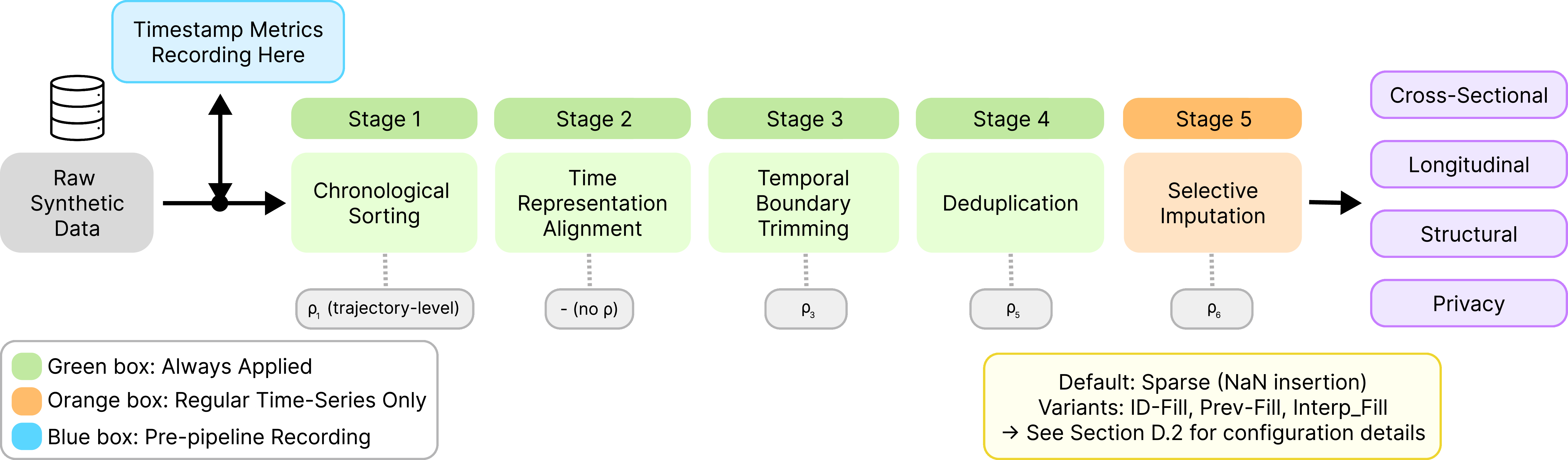
As discussed in the main paper, we apply a deterministic five-stage pipeline to repair temporal violations (e.g., chronological ordering, calendar alignment) before computing non-timestamp metrics. Figure 5 provides a comprehensive visual overview of this sequence, illustrating how raw synthetic outputs are progressively sorted, aligned, trimmed, deduplicated, and optionally imputed.
9.1 Detailed Pipeline Stages↩︎
Generative models that treat timestamps as ordinary features frequently emit outputs that violate the preconditions assumed by non-timestamp metrics: chronological ordering, calendar alignment, and gap-free trajectories. We apply a deterministic five-stage pipeline to repair these violations before computing non-timestamp metrics; timestamp metrics, by contrast, are computed on the raw synthetic output so that violations are not masked by the corrections themselves. At each stage we log the intervention ratio \(\rho_s = (N^{\text{mod}}_s + N^{\text{drop}}_s)/N^{\text{in}}_s\), the fraction of records modified or dropped, as an auxiliary signal of temporal-coherence failure.
9.1.0.1 Stages (in dependency order).
(1) Sort: records sorted ascending by \((x^{key}, x^{time})\). (2) Time Alignment: synthetic timestamps snapped to the canonical grid at interval \(c\); non-calendar outputs are anchored at the earliest real period and assigned \(c\)-spaced increments. (3) Temporal Boundary Trimming: records outside the observed support \([T_{\min}, T_{\max}]\) are removed. (4) Deduplication: duplicate \((x^{key}, x^{time})\) pairs are resolved by retaining the first occurrence. (5) Selective Imputation (regular series only): unoccupied grid points within each trajectory’s observed range are filled according to the chosen variant; points outside this range are not imputed.
9.1.0.2 Method variants.
Stages (1)–(4) are deterministic; the four variants differ only in Stage (5)’s imputation: sparse (default; insert as NaN, exposing the model’s coverage pattern as a measurable property); id-fill (within-trajectory mean/mode); prev-fill (forward-fill, backward-fill for leading gaps); interp-fill (linear interpolation for numerical, forward/backward fill for categorical).
9.2 Recommended Configurations↩︎
Among the pipeline steps, only Stages (2) and (5) require configuration. For Stage 2, calendar-aligned synthetic timestamps are anchored to canonical period boundaries (e.g., first day of the month) rather than nearest-neighbor rounding, guaranteeing
membership in the grid required by GridCompleteness. For Stage 5, we strongly recommend the sparse variant as the default. Standard imputations (id-fill, prev-fill, interp-fill) inject in-distribution values, mechanically inflating fidelity scores and concealing a model’s failure to maintain temporal coverage. While these fill variants serve as useful
ablation baselines for evaluating feature-level fidelity conditional on complete coverage (detailed in Section 10.2), the intervention ratio \(\rho_5\) must always
be reported alongside metric scores to ensure transparency.
10 Experimental Details↩︎
10.1 Baseline Training Setup & Hardware↩︎
To ensure fair reproducibility, all generative models were trained using default hyperparameters and configurations from their official repositories or the SyntheRela benchmark [9]. For baseline dataset preprocessing, we applied a uniform pipeline: numerical missing values were mean-imputed (rounded for integers), categorical gaps were filled with a placeholder (‘?’), and hash-based IDs were globally integerized to maintain relational integrity. Excessively large datasets were subsampled at the trajectory (primary key) level for computational feasibility. All experiments were executed on a server equipped with NVIDIA RTX 6000 Ada GPUs.
10.2 Imputation Sensitivity Analysis↩︎
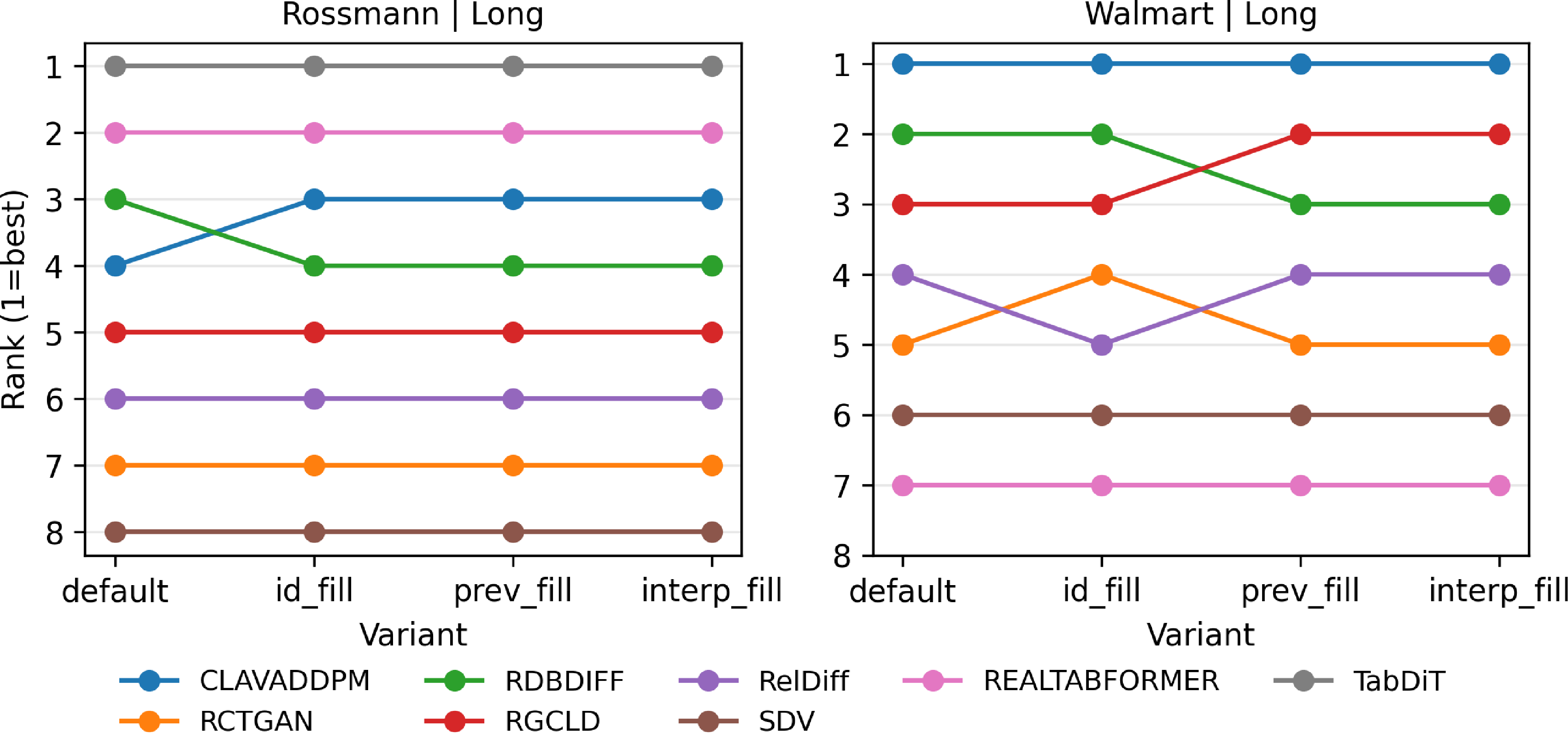
We conduct an ablation study to empirically validate that the choice of imputation strategy (Stage 5) does not materially alter the comparative conclusions drawn from Seq2Synth. Specifically, we compare four variants — sparse (default, missing grid points left as NaN), id-fill (within-trajectory mean/mode), prev-fill (forward-fill with backward-fill for leading gaps), and interp-fill (linear interpolation for numerical; forward/backward fill for categorical) — across representative regular datasets, Rossmann and Walmart. Imputation variants are applicable only to regular-series datasets; for irregular-series datasets (Airbnb, Berka) and the PTB-XL ECG dataset, which involve independent trajectories or sparse event structures, the evaluation reduces to the sparse baseline and a single “default” point is shown.
10.2.0.1 Protocol.
For each dataset \(d\), metric group \(m \in \{\text{SD}, \text{CS}, \text{Long}, \text{Struct}\}\), and imputation variant \(v\), we compute each model’s rank (1 = best) within the set of evaluated models. Model ranks are then tracked across imputation variants. A stable rank profile indicates that the relative ordering of models — and thus the benchmark’s comparative conclusions — is insensitive to the imputation choice.
10.2.0.2 Results.
Figure 6 shows model ranks per dataset and metric group under all applicable imputation variants. The key observation is that rank orderings remain largely stable across variants for the majority of dataset–metric combinations. Rank crossings, when they occur, are almost exclusively between models that are already closely ranked under the default setting, reflecting genuine measurement noise rather than a systematic artefact of imputation. No imputation variant consistently elevates or demotes a specific model across datasets, and models that rank near the top (or bottom) under sparse tend to maintain their relative position under all three fill-based alternatives.
This stability holds across both feature-sensitive metric groups (Cross-Sectional, Longitudinal) and structure-sensitive ones (Structural), indicating that the effect of filling missing grid points with in-distribution values does not substantially inflate or suppress any model’s score relative to its competitors. The result is consistent with our theoretical expectation: because all models are subject to the same imputation procedure, the filling introduces a uniform bias that cancels in comparative analysis.
For irregular-series and independent-trajectory datasets (PTB-XL), which are evaluated only under sparse, ranks are determined solely by the model’s ability to generate the correct temporal support, confirming that imputation is not a confound for these data types.
10.2.0.3 Implications.
These results jointly support two claims. First, the sparse default is empirically justified: adopting any of the three fill-based alternatives leads to the same comparative conclusions while introducing unnecessary feature-level bias as discussed in Section 9.2. Second, the metrics themselves are robust: they quantify genuine model-level differences in temporal fidelity rather than artefacts of the post-processing pipeline. Together, these findings validate both the imputation design choice and the metric computations reported in the main paper.
10.3 Detailed Dataset Statistics↩︎
To provide a comprehensive operational overview of our evaluation testbed, Table ¿tbl:tab:dataset95statistics? summarizes the structural dimensions of the 13 sequential tabular datasets, including the total number of relational tables, absolute rows, schema columns, unique entity trajectories, and the resulting average trajectory length.
| Dataset | # tables | # rows | # columns | # trajectories | avg traj. length |
|---|---|---|---|---|---|
| Walmart | 3 | 15,317 | 20 | 45 | 334.38 |
| PTB-XL | 2 | 101,000 | 35 | 1,000 | 100 |
| FreddieMAC | 2 | 536,578 | 39 | 43,966 | 11.20 |
| FannieMAE | 2 | 2,992,782 | 47 | 183,777 | 15.28 |
| H&M | 3 | 297,879 | 36 | 10,000 | 24.03 |
| Coupon | 5 | 259,833 | 38 | 22,873 | 5.41 |
| 5 | 756,167 | 47 | 498 | 1,019.20 | |
| Home Credit | 7 | 1,263,300 | 218 | 10,000 | 36.35 |
| Rossmann | 2 | 13,826 | 20 | 223 | 61.00 |
| AirBnB | 2 | 40,281 | 32 | 1,942 | 19.74 |
| Berka | 2 | 45,666 | 19 | 900 | 49.74 |
| CMAPSS | 1 | 160,359 | 26 | 709 | 226.18 |
| Citi Bike | 1 | 559,644 | 15 | 5,793 | 96.61 |
10.4 Per-Dataset Description↩︎
We evaluate our benchmark on a diverse set of real-world sequential tabular datasets, selected to cover a wide range of temporal characteristics, relational structures, and application domains.
Walmart We use the subsampled versions of Walmart and Rossmann datasets used in SyntheRela [9]. Both datasets exhibit regular, absolute timestamps with fixed-length trajectories.
H&M Personalized Fashion Recommendations. H&M [23] contains customer purchase records over time, along with auxiliary information on users and items. It features a relational schema with two parent tables and one child table, posing challenges for models that cannot handle multi-parent dependencies (e.g., RTF).
Coupon Purchase Prediction. The Coupon dataset [24] includes user profiles, coupon metadata, browsing logs, and purchase events. It has a multi-parent, multi-child relational structure with 2-hop dependencies, making it suitable for evaluating relational consistency across multiple tables.
PTB-XL. PTB-XL [25] consists of electrocardiography (ECG) signals collected at high temporal resolution. It is suitable for evaluating synthetic data generation in the healthcare domain, where privacy preservation and realistic temporal modeling are critical. Each record forms a fixed-length time series, allowing evaluation of models on dense and high-frequency temporal data.
Freddie Mac and Fannie MAE. The Freddie Mac dataset [26] provides loan-level mortgage performance data spanning multiple decades while Fannie MAE [27] contains detailed records of single-family mortgage loans.
Home Credit Default Risk. The Home Credit dataset [28] provides transactional and application data for credit risk prediction. Notably, the application table contains over 120 features, allowing evaluation of high-dimensional tabular generation.
Google Cluster Traces v2. This dataset [29] records task execution traces from a large-scale cluster system. Time is represented in relative units (600-second intervals), and each task forms a temporal sequence, enabling evaluation under system-level workload dynamics.
CMAPSS. CMAPSS [30] is a simulated dataset of aircraft engine degradation trajectories. Each sequence evolves over relative time cycles, making it suitable for evaluating temporal progression and failure patterns.
Citi Bike NYC. The Citi Bike dataset [31] contains trip-level records with absolute timestamps. Each trajectory corresponds to a bike usage session, allowing evaluation of real-world mobility patterns with irregular temporal spacing.
AirBnB, Berka and Rossmann The AirBnB dataset [11] includes temporally ordered reservation records together with static listing attributes, enabling evaluation of models on relational data with heterogeneous temporal patterns and sparse event occurrences. The Berka dataset [11] is a financial relational dataset consisting of customer accounts, transactions, loans, and demographic information. Transaction histories evolve over absolute time and exhibit long-term sequential dependencies, making the dataset suitable for evaluating temporal consistency and relational coherence in synthetic financial records. The Rossmann dataset [11] contains daily sales records from retail stores along with static store metadata and promotion-related information. Each store forms a fixed-frequency temporal trajectory with regular daily intervals, allowing evaluation of seasonal patterns, trend preservation, and long-range temporal dependencies in retail forecasting scenarios.
10.5 Preprocessing Details per Dataset↩︎
Baseline missing-value preprocessing is described in Section 10.1; temporal post-processing is described in Section 9.
10.5.0.1 Retail Domain.
We utilize the subsampled version Walmart provided by SyntheRela [9]. For Rossmann, AirBnB, and Berka, we consider test-set splits that authors of TabDiT [11] provided are used as the real datasets for evaluating all seven baseline models, while TabDiT-generated samples are directly used. For H&M, we randomly subsample 10,000 customers from the original customer IDs. Image-related information is excluded, and only the corresponding subsampled article metadata is retained in the articles table.
10.5.0.2 Medical Domain.
PTB-XL is preprocessed using the official pipeline provided by the source dataset and then decomposed into a parent-child relational structure, where metadata is stored in the parent table and ECG signals are stored in the child table. We use the 100Hz
recordings, for which each ecg_id originally contains 1,000 temporal observations. Since generated data may not reliably preserve microsecond-level temporal precision, we introduce a relative timestep column (step) to represent
temporal ordering explicitly. We further apply temporal downsampling to reduce each trajectory to 100 timesteps for more stable and computationally efficient benchmarking. A total of 1,000 ecg_ids are randomly subsampled. Columns with high
missing-value ratios are removed to improve robustness.
10.5.0.3 Finance Domain.
For Freddie Mac and Fannie Mae, we use loan records reported after 2024. In the case of Fannie Mae, the original single-table structure is transformed into a relational schema by separating static loan attributes into a parent table and time-varying records into a child table. For Home Credit Default Risk, 10,000 IDs are randomly subsampled from the full dataset.
10.5.0.4 Other Domains.
For Google Cluster Traces v2, we use the first five shards and randomly subsample 500 machine IDs. To establish a relational schema with a designated primary entity, static job-level attributes are separated from event logs to construct a root table
named jobs. This restructuring is not applicable to machine events because they contain only static information; therefore, the machine events and machine attribute tables are excluded. For CMAPSS, the four simulation subsets are merged into a
single unified table.
10.6 MLD-TS and MLE-TS Evaluation Details↩︎
| Hyperparameter | Value |
|---|---|
| max_depth | \(\{3, 5, 7, 9\}\) |
| learning_rate | \(\{0.01, 0.03, 0.05, 0.10\}\) |
| min_child_weight | \(\{1, 3\}\) |
| n_estimators | \(\{50\}\) |
We used XGBoost [32] for both MLD-TS and MLE-TS evaluations. In MLD-TS, real and synthetic samples were combined and then split into training and test sets with a ratio of 8:2. The model was trained as a binary classifier to distinguish real samples from synthetic samples, and accuracy was used as the evaluation metric. In MLE-TS, the training set was constructed using only synthetic data, while the test set consisted only of real data, following the same 8:2 split ratio. For each random seed, hyperparameters were randomly sampled from a predefined search space summarized in Table 8.
10.6.0.1 Downstream Tasks for MLE-TS.
Since MLE-TS evaluates whether synthetic data preserves the predictive structure of real data, it requires a target label for each sample. For datasets where the original target label is not directly available, we define binary prediction tasks using attributes from the corresponding parent, store, customer, or entity-level tables. Specifically:
In Airbnb, we define the task
n_sessions_ge_17. The target label is set to 1 ifn_sessionsis greater than or equal to 17, and 0 otherwise.In Berka, we define the task
region_is_moravia. The target label is set to 1 if the customer’s region is either South Moravia or North Moravia, and 0 otherwise.In Citi Bike, we define the task
mode_gender_is_1. For each bike, we compute the mode ofgenderacross its records and set the target label to 1 if the modal value is 1, and 0 otherwise.In CMAPSS, we define the task
final_s11_high_regime. For each unit, we use the value ofs_11at the final time step and predict whether it is greater than or equal to the median value computed from the real data.In Coupon, we define the task
sex_is_m. The target label is set to 1 ifsexis male, and 0 otherwise.In Fannie Mae, and Freddie Mac, we define the task . The target label is set to 1 if the corresponding property-type field is equal to 4, and 0 otherwise.
In Google Cluster, we define the task . The target label is set to 1 if
scheduling_classis greater than or equal to 2, and 0 otherwise.In H&M, we use the binary attribute as the target label.
In Home Credit, we use the binary attribute
TARGETas the target label.In PTB-XL, we use the binary attribute
sexas the target label.In Rossmann, we use the binary attribute
Promo2from the store table. The target label is set to 1 ifPromo2is equal to 1, and 0 otherwise.In Walmart, we define the task . The target label is set to 1 if the store type
Typeis “A”, and 0 otherwise.
11 Additional Results↩︎
11.1 Results on Additional Dataset↩︎
Additional results on single-table and complex datasets. Tables ¿tbl:tab:single95table95results? and ¿tbl:tab:complex95data95results? report the remaining dataset-level results beyond the seven core datasets.
width=
The single-table datasets confirm that temporal fidelity remains multi-dimensional even without explicit inter-table relationships. On Citi Bike, ClavaDDPM leads static and cross-sectional fidelity, RTF leads longitudinal fidelity, and RCTGAN/SDV achieve the strongest structural scores. On CMAPSS, TabularARGN obtains the best static-distribution score, whereas CPAR, RTF, and SDV lead timestamp, longitudinal, and structural fidelity, respectively. Thus, even in single-table settings, no single dimension summarizes overall temporal quality.
width=, max totalheight=0.3 width=, max totalheight=0.3
The complex-schema datasets further amplify this pattern. On Coupon, RDBDiff dominates static, timestamp, and structural fidelity, while RelDiff achieves the best longitudinal score. On Google Cluster, diffusion-based relational models preserve structural consistency well, but their longitudinal scores remain moderate. On H&M and Home Credit, graph- and diffusion-based methods such as RGCLD, RDBDiff, and RelDiff generally perform strongly, but the best model still changes across dimensions. These results show that complex schemas introduce additional failure modes: preserving relational structure does not guarantee faithful timestamp generation or trajectory evolution, and static-distribution fidelity remains insufficient as a proxy for temporal quality.
| Dataset | Metric | ClavaDDPM | RCTGAN | RDBDiff | RelDiff | RGCLD | RTF | SDV | TabDiT | CPAR | TabARGN |
|---|---|---|---|---|---|---|---|---|---|---|---|
| Rossmann | sd | 0.850 | 0.810 | \(\underline{0.858}\) | 0.799 | 0.821 | 0.809 | 0.734 | \(\mathbf{0.932}\) | – | – |
| ts | 0.607 | 0.562 | 0.608 | 0.602 | 0.598 | \(\underline{0.823}\) | 0.565 | \(\mathbf{0.824}\) | – | – | |
| cs | \(\underline{0.912}\) | 0.808 | \(\underline{0.912}\) | 0.817 | 0.897 | 0.882 | 0.635 | \(\mathbf{0.965}\) | – | – | |
| lg | 0.917 | 0.872 | 0.915 | 0.882 | 0.902 | \(\underline{0.948}\) | 0.789 | \(\mathbf{0.975}\) | – | – | |
| st | \(\mathbf{1.000}\) | \(\mathbf{1.000}\) | \(\mathbf{1.000}\) | \(\mathbf{1.000}\) | \(\mathbf{1.000}\) | \(\mathbf{1.000}\) | \(\mathbf{1.000}\) | \(\mathbf{1.000}\) | – | – | |
| Berka | sd | 0.948 | 0.865 | \(\mathbf{0.992}\) | 0.898 | 0.922 | \(\underline{0.951}\) | 0.695 | 0.909 | – | – |
| ts | 0.594 | 0.620 | 0.759 | 0.603 | 0.731 | \(\mathbf{0.907}\) | 0.535 | \(\underline{0.777}\) | – | – | |
| cs | \(\underline{0.691}\) | 0.632 | \(\mathbf{0.829}\) | 0.626 | 0.671 | 0.665 | 0.448 | 0.651 | – | – | |
| lg | 0.877 | 0.858 | \(\mathbf{0.949}\) | 0.868 | 0.885 | \(\underline{0.896}\) | 0.686 | 0.890 | – | – | |
| st | 0.993 | 0.952 | \(\mathbf{1.000}\) | \(\mathbf{1.000}\) | 0.993 | 0.952 | 0.814 | 0.958 | – | – | |
| Fannie Mae | sd | \(\underline{0.900}\) | 0.860 | 0.876 | 0.899 | \(\mathbf{0.906}\) | 0.854 | 0.814 | – | – | – |
| ts | 0.567 | 0.550 | \(\underline{0.571}\) | \(\mathbf{0.598}\) | 0.503 | 0.474 | 0.481 | – | – | – | |
| cs | \(\mathbf{0.965}\) | 0.852 | 0.870 | 0.849 | \(\underline{0.876}\) | 0.777 | 0.772 | – | – | – | |
| lg | 0.820 | 0.787 | 0.781 | 0.822 | \(\underline{0.858}\) | 0.804 | \(\mathbf{0.864}\) | – | – | – | |
| st | \(\mathbf{0.998}\) | 0.953 | 0.822 | 0.750 | \(\underline{0.990}\) | 0.817 | 0.848 | – | – | – | |
| Walmart | sd | 0.796 | 0.861 | 0.815 | \(\underline{0.898}\) | \(\mathbf{0.950}\) | 0.719 | 0.857 | – | – | – |
| ts | \(\mathbf{0.610}\) | 0.526 | \(\underline{0.608}\) | 0.598 | 0.600 | 0.455 | 0.522 | – | – | – | |
| cs | 0.867 | 0.785 | \(\mathbf{0.896}\) | 0.828 | \(\underline{0.891}\) | 0.605 | 0.746 | – | – | – | |
| lg | \(\mathbf{0.887}\) | 0.844 | 0.868 | 0.852 | \(\underline{0.872}\) | 0.690 | 0.814 | – | – | – | |
| st | 0.864 | 0.731 | \(\mathbf{0.887}\) | 0.804 | \(\underline{0.882}\) | 0.518 | 0.786 | – | – | – | |
| Airbnb | sd | \(\mathbf{0.967}\) | 0.909 | \(\underline{0.963}\) | 0.937 | 0.925 | 0.879 | 0.711 | 0.923 | – | – |
| ts | \(\mathbf{0.875}\) | 0.840 | 0.824 | \(\underline{0.860}\) | 0.843 | 0.777 | 0.811 | \(\underline{0.860}\) | – | – | |
| cs | – | – | – | – | – | – | – | – | – | – | |
| lg | 0.964 | \(\mathbf{0.970}\) | 0.965 | \(\underline{0.969}\) | \(\underline{0.969}\) | 0.967 | 0.909 | 0.965 | – | – | |
| st | 0.987 | 0.924 | \(\mathbf{1.000}\) | \(\mathbf{1.000}\) | 0.981 | 0.631 | 0.938 | 0.912 | – | – | |
| PTB-XL | sd | \(\underline{0.886}\) | 0.576 | \(\mathbf{0.896}\) | 0.669 | 0.692 | 0.625 | 0.758 | – | – | – |
| ts | 0.594 | 0.330 | 0.577 | 0.591 | 0.534 | \(\mathbf{1.000}\) | \(\underline{0.675}\) | – | – | – | |
| cs | – | – | – | – | – | – | – | – | – | – | |
| lg | \(\mathbf{0.927}\) | 0.841 | 0.909 | \(\underline{0.922}\) | 0.906 | 0.915 | 0.920 | – | – | – | |
| st | \(\mathbf{1.000}\) | \(\mathbf{1.000}\) | \(\mathbf{1.000}\) | \(\mathbf{1.000}\) | \(\mathbf{1.000}\) | 0.999 | \(\mathbf{1.000}\) | – | – | – | |
| Freddie Mac | sd | 0.944 | 0.882 | \(\mathbf{0.986}\) | 0.920 | \(\underline{0.975}\) | 0.853 | 0.810 | – | – | – |
| ts | 0.713 | 0.688 | 0.660 | \(\mathbf{0.752}\) | 0.736 | 0.581 | \(\underline{0.747}\) | – | – | – | |
| cs | 0.924 | 0.843 | \(\mathbf{0.982}\) | 0.847 | \(\underline{0.930}\) | 0.777 | 0.740 | – | – | – | |
| lg | 0.842 | 0.797 | \(\mathbf{0.915}\) | 0.841 | \(\underline{0.875}\) | 0.784 | 0.780 | – | – | – | |
| st | 0.995 | 0.972 | \(\mathbf{1.000}\) | \(\mathbf{1.000}\) | 0.993 | 0.695 | 0.965 | – | – | – | |
| Coupon | sd | \(\underline{0.895}\) | 0.894 | \(\mathbf{0.976}\) | 0.881 | 0.863 | – | 0.827 | – | – | – |
| ts | 0.828 | 0.817 | \(\mathbf{0.896}\) | \(\underline{0.848}\) | 0.606 | – | 0.805 | – | – | – | |
| cs | \(\mathbf{0.801}\) | \(\underline{0.798}\) | 0.789 | 0.779 | 0.737 | – | 0.474 | – | – | – | |
| lg | 0.636 | 0.626 | 0.668 | \(\mathbf{0.908}\) | 0.674 | – | \(\underline{0.837}\) | – | – | – | |
| st | 0.974 | 0.930 | \(\mathbf{0.987}\) | \(\underline{0.979}\) | 0.949 | – | 0.895 | – | – | – | |
| Google Cluster | sd | \(\underline{0.863}\) | 0.715 | \(\mathbf{0.935}\) | 0.781 | 0.706 | – | 0.599 | – | – | – |
| ts | 0.604 | 0.574 | 0.627 | \(\underline{0.645}\) | \(\mathbf{0.650}\) | – | 0.630 | – | – | – | |
| cs | – | – | – | – | – | – | – | – | – | – | |
| lg | 0.481 | 0.457 | \(\underline{0.507}\) | 0.455 | \(\mathbf{0.516}\) | – | 0.486 | – | – | – | |
| st | 0.977 | 0.708 | \(\mathbf{1.000}\) | \(\mathbf{1.000}\) | 0.986 | – | 0.567 | – | – | – | |
| H&M | sd | \(\mathbf{0.933}\) | 0.626 | \(\underline{0.891}\) | 0.871 | 0.871 | – | 0.641 | – | – | – |
| ts | 0.680 | \(\mathbf{0.709}\) | 0.682 | 0.688 | \(\underline{0.704}\) | – | 0.581 | – | – | – | |
| cs | 0.820 | 0.521 | 0.789 | \(\underline{0.842}\) | \(\mathbf{0.874}\) | – | 0.456 | – | – | – | |
| lg | \(\underline{0.873}\) | 0.715 | 0.756 | 0.772 | \(\mathbf{0.876}\) | – | 0.680 | – | – | – | |
| st | \(\underline{0.640}\) | 0.555 | 0.638 | \(\underline{0.640}\) | \(\underline{0.640}\) | – | \(\mathbf{0.648}\) | – | – | – | |
| Home Credit | sd | 0.671 | 0.850 | \(\mathbf{0.896}\) | 0.826 | \(\underline{0.860}\) | – | – | – | – | – |
| ts | 0.628 | 0.611 | \(\underline{0.690}\) | 0.671 | \(\mathbf{0.719}\) | – | – | – | – | – | |
| cs | – | – | – | – | – | – | – | – | – | – | |
| lg | 0.916 | 0.888 | \(\underline{0.935}\) | 0.910 | \(\mathbf{0.937}\) | – | – | – | – | – | |
| st | 0.953 | 0.870 | \(\underline{0.996}\) | \(\mathbf{1.000}\) | 0.994 | – | – | – | – | – | |
| Citi Bike | sd | \(\mathbf{0.990}\) | \(\underline{0.943}\) | – | – | – | 0.870 | 0.883 | – | 0.706 | 0.890 |
| ts | \(\underline{0.769}\) | 0.765 | – | – | – | 0.678 | \(\mathbf{0.782}\) | – | 0.721 | 0.201 | |
| cs | \(\mathbf{0.941}\) | \(\underline{0.900}\) | – | – | – | 0.885 | 0.848 | – | 0.614 | 0.757 | |
| lg | \(\underline{0.965}\) | 0.960 | – | – | – | \(\mathbf{0.967}\) | 0.950 | – | 0.811 | 0.921 | |
| st | 0.908 | \(\mathbf{0.979}\) | – | – | – | 0.676 | \(\mathbf{0.979}\) | – | 0.271 | 0.154 | |
| CMAPSS | sd | 0.963 | 0.813 | – | – | – | \(\underline{0.972}\) | 0.916 | – | 0.811 | \(\mathbf{0.983}\) |
| ts | 0.575 | 0.369 | – | – | – | 0.322 | 0.545 | – | \(\mathbf{0.969}\) | \(\underline{0.578}\) | |
| cs | – | – | – | – | – | – | – | – | – | – | |
| lg | 0.471 | 0.459 | – | – | – | \(\mathbf{0.618}\) | 0.425 | – | \(\underline{0.573}\) | 0.485 | |
| st | 0.709 | 0.330 | – | – | – | 0.000 | \(\mathbf{0.961}\) | – | 0.836 | \(\underline{0.917}\) |
2.0pt
11.2 MLE-TS↩︎
| Dataset | Original | ClavaDDPM | CPAR | RCTGAN | RTF | SDV | RDBDIFF | RGCLD | RelDiff | TABARGN | TabDiT |
|---|---|---|---|---|---|---|---|---|---|---|---|
| Rossmann | \(0.806\) | \(0.771\) | – | \(0.314\) | \(0.500\) | \(0.533\) | \(0.749\) | \(0.778\) | \(0.708\) | – | \(\mathbf{0.782}\) |
| Berka | \(0.502\) | \(0.445\) | – | \(0.480\) | \(0.511\) | \(0.467\) | \(0.492\) | \(0.550\) | \(\mathbf{0.557}\) | – | \(0.438\) |
| Fannie Mae | \(0.685\) | \(0.601\) | – | \(0.533\) | \(0.628\) | \(0.602\) | \(0.622\) | \(0.654\) | \(\mathbf{0.658}\) | – | – |
| Walmart | \(0.717\) | \(\mathbf{0.867}\) | – | \(0.550\) | \(0.767\) | \(0.733\) | \(0.833\) | \(0.792\) | \(0.500\) | – | – |
| Airbnb | \(1.000\) | \(0.806\) | – | \(0.881\) | \(0.624\) | \(0.978\) | \(\mathbf{1.000}\) | \(1.000\) | \(0.930\) | – | \(\mathbf{1.000}\) |
| PTB-XL | \(0.712\) | \(0.473\) | – | \(0.476\) | \(\mathbf{0.672}\) | \(0.500\) | \(0.515\) | \(0.524\) | \(0.446\) | – | – |
| Freddie Mac | \(0.691\) | \(0.486\) | – | \(0.519\) | \(0.572\) | \(0.500\) | \(0.504\) | \(\mathbf{0.664}\) | \(0.596\) | – | – |
| Citi Bike | \(0.994\) | \(0.995\) | \(\mathbf{0.996}\) | \(0.839\) | \(0.995\) | \(0.836\) | – | – | – | \(0.669\) | – |
| CMAPSS | \(0.848\) | \(0.757\) | \(0.500\) | \(0.475\) | \(0.757\) | \(\mathbf{0.820}\) | – | – | – | \(0.771\) | – |
| Coupon | \(0.679\) | \(0.577\) | – | \(0.507\) | – | \(0.527\) | \(0.542\) | \(\mathbf{0.645}\) | \(0.610\) | – | – |
| Google Cluster | \(0.950\) | \(0.828\) | – | \(0.616\) | – | \(0.437\) | \(\mathbf{0.885}\) | \(0.790\) | \(0.725\) | – | – |
| H&M | \(0.602\) | \(\mathbf{0.585}\) | – | \(0.479\) | – | \(0.536\) | \(0.579\) | \(0.577\) | \(0.574\) | – | – |
| Home Credit | \(0.590\) | \(0.467\) | – | \(0.460\) | – | – | \(0.517\) | \(\mathbf{0.573}\) | \(0.530\) | – | – |
3pt
Table 10 summarizes downstream temporal utility on the MLE-TS benchmark. The best synthetic generators often approach, and sometimes surpass, the real-data baseline, showing that synthetic data can support downstream temporal prediction when it preserves task-relevant patterns rather than only marginal distributions. At the same time, utility remains highly dataset-dependent: no method consistently dominates, and larger gaps on datasets with complex temporal dynamics and heterogeneous feature interactions suggest that current generators still struggle to reproduce fine-grained predictive structure. This highlights the need to evaluate synthetic data not only by distributional fidelity, but also by whether it transfers useful temporal signals to downstream tasks.
11.3 MLE-Temporal↩︎
| Dataset | Metric | Model | Performance |
|---|---|---|---|
| Rossmann | \(R^2\) | ClavaDDPM | 0.577 |
| \(R^2\) | RCTGAN | 0.422 | |
| \(R^2\) | RDBDIFF | 0.530 | |
| \(R^2\) | RTF | 0.285 | |
| \(R^2\) | RelDiff | 0.187 | |
| \(R^2\) | RGCLD | 0.571 | |
| \(R^2\) | SDV | \(-64.945\) | |
| \(R^2\) | TabDiT | 0.578 | |
| Fannie Mae | AUC | ClavaDDPM | 0.502 |
| AUC | RCTGAN | 0.702 | |
| AUC | RDBDIFF | 0.781 | |
| AUC | RTF | 0.852 | |
| AUC | RelDiff | 0.924 | |
| AUC | RGCLD | 0.890 | |
| AUC | SDV | 0.913 | |
| Walmart | \(R^2\) | ClavaDDPM | 0.355 |
| \(R^2\) | RCTGAN | 0.247 | |
| \(R^2\) | RDBDIFF | 0.475 | |
| \(R^2\) | RTF | 0.104 | |
| \(R^2\) | RelDiff | \(-0.014\) | |
| \(R^2\) | RGCLD | 0.516 | |
| \(R^2\) | SDV | 0.012 | |
| Freddie Mac | AUC | ClavaDDPM | 0.596 |
| AUC | RCTGAN | 0.643 | |
| AUC | RDBDIFF | 0.686 | |
| AUC | RTF | 0.527 | |
| AUC | RelDiff | 0.848 | |
| AUC | RGCLD | 0.869 | |
| AUC | SDV | 0.500 |
5pt
Table 11 reports MLE-Temporal results under a chronological train/test split, where models are trained on earlier observations and evaluated on later ones. This setting provides a stricter test than the random-split MLE-TS protocol because synthetic data must support forward-looking temporal prediction. On the binary classification tasks, RelDiff and RGCLD obtain the best AUC scores on Fannie Mae and Freddie Mac, respectively, with SDV also performing strongly on Fannie Mae. In contrast, the regression tasks show weaker utility: the best \(R^2\) values on Rossmann and Walmart remain moderate, and some generators produce near-zero or negative scores. This contrast suggests that current generators can preserve coarse temporal signals useful for classification more reliably than the fine-grained continuous dynamics required for temporal forecasting.
11.4 MLD-TS↩︎
| Dataset | Setting | Original | ClavaDDPM | CPAR | RCTGAN | RTF | SDV | RDBDIFF | RGCLD | RelDiff | TABARGN | TabDiT |
|---|---|---|---|---|---|---|---|---|---|---|---|---|
| Airbnb | child | \(0.503\) | \(0.964\) | – | \(0.987\) | \(0.897\) | \(1.000\) | \(0.988\) | \(0.879\) | \(0.889\) | – | \(\mathbf{0.852}\) |
| merged | \(0.499\) | \(0.965\) | – | \(0.987\) | \(0.929\) | \(1.000\) | \(0.987\) | \(\mathbf{0.879}\) | \(0.912\) | – | \(0.947\) | |
| Berka | child | \(0.498\) | \(0.964\) | – | \(0.990\) | \(0.672\) | \(0.999\) | \(\mathbf{0.532}\) | \(0.738\) | \(0.988\) | – | \(0.862\) |
| merged | \(0.493\) | \(0.965\) | – | \(0.990\) | \(0.669\) | \(0.999\) | \(\mathbf{0.523}\) | \(0.741\) | \(0.988\) | – | \(0.861\) | |
| Citi Bike | child | \(0.499\) | \(\mathbf{0.804}\) | \(1.000\) | \(0.970\) | \(0.956\) | \(0.997\) | – | – | – | \(0.992\) | – |
| merged | \(0.499\) | \(\mathbf{0.804}\) | \(1.000\) | \(0.970\) | \(0.956\) | \(0.997\) | – | – | – | \(0.992\) | – | |
| CMAPSS | child | \(0.502\) | \(0.997\) | \(1.000\) | \(0.997\) | \(\mathbf{0.976}\) | \(0.998\) | – | – | – | \(0.981\) | – |
| merged | \(0.502\) | \(0.997\) | \(1.000\) | \(0.997\) | \(\mathbf{0.976}\) | \(0.998\) | – | – | – | \(0.981\) | – | |
| Coupon | child | \(0.499\) | \(0.842\) | – | \(0.878\) | – | \(0.965\) | \(\mathbf{0.758}\) | \(0.812\) | \(0.881\) | – | – |
| merged | \(0.498\) | \(0.841\) | – | \(0.879\) | – | \(0.965\) | \(\mathbf{0.759}\) | \(0.808\) | \(0.881\) | – | – | |
| Fannie Mae | child | \(0.499\) | \(1.000\) | – | \(1.000\) | \(\mathbf{0.838}\) | \(1.000\) | \(1.000\) | \(1.000\) | \(1.000\) | – | – |
| merged | \(0.500\) | \(1.000\) | – | \(1.000\) | \(\mathbf{0.840}\) | \(1.000\) | \(1.000\) | \(1.000\) | \(1.000\) | – | – | |
| Freddie Mac | child | \(0.502\) | \(1.000\) | – | \(1.000\) | \(0.999\) | \(1.000\) | \(1.000\) | \(\mathbf{0.966}\) | \(0.996\) | – | – |
| merged | \(0.502\) | \(1.000\) | – | \(1.000\) | \(0.999\) | \(1.000\) | \(1.000\) | \(\mathbf{0.966}\) | \(0.996\) | – | – | |
| Google Cluster | child | \(0.503\) | \(0.964\) | – | \(0.996\) | – | \(0.999\) | \(0.915\) | \(\mathbf{0.798}\) | \(0.976\) | – | – |
| merged | \(0.500\) | \(0.965\) | – | \(0.996\) | – | \(0.999\) | \(0.915\) | \(\mathbf{0.802}\) | \(0.976\) | – | – | |
| H&M | child | \(0.495\) | \(0.734\) | – | \(0.986\) | – | \(1.000\) | \(0.903\) | \(\mathbf{0.712}\) | \(0.736\) | – | – |
| merged | \(0.496\) | \(\mathbf{0.735}\) | – | \(0.986\) | – | \(1.000\) | \(0.903\) | \(0.902\) | \(0.907\) | – | – | |
| Home Credit | child | \(0.496\) | \(0.928\) | – | \(0.919\) | – | – | \(0.999\) | \(\mathbf{0.691}\) | \(0.812\) | – | – |
| merged | \(0.497\) | \(1.000\) | – | \(0.981\) | – | – | \(0.999\) | \(\mathbf{0.732}\) | \(0.849\) | – | – | |
| PTB-XL | child | \(0.501\) | \(1.000\) | – | \(1.000\) | \(1.000\) | \(1.000\) | \(\mathbf{0.858}\) | \(0.988\) | \(0.994\) | – | – |
| merged | \(0.491\) | \(1.000\) | – | \(1.000\) | \(1.000\) | \(1.000\) | \(\mathbf{0.861}\) | \(0.994\) | \(0.994\) | – | – | |
| Rossmann | child | \(0.502\) | \(0.997\) | – | \(0.985\) | \(0.984\) | \(0.997\) | \(0.986\) | \(0.984\) | \(0.998\) | – | \(\mathbf{0.825}\) |
| merged | \(0.504\) | \(0.997\) | – | \(0.990\) | \(0.984\) | \(0.997\) | \(0.985\) | \(0.986\) | \(0.998\) | – | \(\mathbf{0.817}\) | |
| Walmart | child | \(0.548\) | \(0.989\) | – | \(0.989\) | \(0.982\) | \(0.989\) | \(0.978\) | \(\mathbf{0.970}\) | \(0.989\) | – | – |
| merged | \(0.533\) | \(0.989\) | – | \(0.989\) | \(0.982\) | \(0.989\) | \(0.978\) | \(\mathbf{0.970}\) | \(0.989\) | – | – |
2pt
Table 12 reports the detection accuracy of the MLD-TS classifier across all datasets, for both the child setting (child table only) and the merged setting (child joined with parent attributes). Lower accuracy indicates that real and synthetic records are harder to distinguish, and therefore that the synthetic data better reproduce the joint structure of the real records. The real-data baseline lies near \(0.5\) across all datasets, confirming that the classifier is not exploiting trivial artifacts. In contrast, most synthetic generators are detected with accuracy well above \(0.95\), indicating that current methods still leave clear distributional fingerprints under a learned discriminator. A few exceptions show measurable progress: RDBDIFF on Berka achieves the lowest detection accuracy (\(0.523\) in the merged setting), and TabDiT on Rossmann (\(0.817\)) and Airbnb (\(0.852\) in the child setting) likewise approach the lower end of the detectability range. RGCLD performs best on several relational datasets (H&M, Home Credit, Walmart), consistent with its competitive temporal fidelity scores reported earlier. Differences between the child and merged settings are generally small, indicating that the detector primarily relies on child-table content rather than on parent–child interactions, and that synthetic-vs-real distinguishability is concentrated in the temporal records themselves. Overall, while MLD-TS confirms that recent relational and temporal generators have narrowed the realism gap on certain datasets, the gap to the real-data baseline remains large, suggesting that distinguishability under learned discriminators is still an open challenge.
11.5 Privacy: Per-Dataset Results↩︎
3pt width=,center
Table ¿tbl:tab:privacy-online? report privacy metric on the remaining six datasets to complement the Rossmann analysis in Section 4.2.0.3. All six metrics follow the higher-is-safer convention;
DCR and CS-DCR are raw median nearest-neighbor distances and are not normalized. For the \(n\)-gram metric we report \(\texttt{NGP}(n)=1-\texttt{NgramExposure}(n)\), so values close to \(1\) indicate that the synthetic data reproduce few real length-\(n\) subsequences.
11.5.0.1 Cross-sectional restriction.
Across the six datasets, \(\texttt{CS-DCR}\) exceeds \(\texttt{DCR}\) on roughly \(90\%\) of model–dataset pairs, confirming that the row-level closeness signal is dominated by neighbors at unrelated time slices. The ratio varies sharply with dataset characteristics: on Berka (long, irregular financial trajectories) the median inflation is \(\sim\!160\times\), on Fannie Mae and Freddie Mac (loan histories) \(\sim\!3\)–\(5\times\), and on PTB-XL (short fixed-length ECG sequences) only \(\sim\!1.8\times\). Walmart is the partial exception: ClavaDDPM has \(\texttt{CS-DCR}\!=\!38.4 < \texttt{DCR}\!=\!42.5\) and RTF has \(\texttt{CS-DCR}\!=\!718.7 < \texttt{DCR}\!=\!779.4\), meaning that same-week nearest neighbors are closer on average than time-agnostic ones—an instance where the row-level metric understates rather than overstates time-aligned identifiability.
11.5.0.2 \(n\)-gram Privacy.
The \(n{=}1\) vs.\(n{=}3\) disagreement seen on Rossmann is dataset-dependent. On datasets with high row vocabulary (Berka, Fannie Mae, Freddie Mac, PTB-XL), NGP(1) already
shows a wide spread among models, so NGP(3) refines rather than overturns the single-token privacy conclusion. On datasets with bounded row vocabulary (Airbnb, Walmart), NGP(1) saturates near the extremes and NGP(3)
is the informative quantity. Across all seven datasets, RTF retains the lowest NGP(3) on five datasets and is in the bottom two on the remaining two, confirming that autoregressive sequence-level reproduction is an architecture-level rather
than a dataset-specific effect.
11.6 Trajectory fidelity.↩︎
| Method | Rossmann | Walmart | PTB-XL |
|---|---|---|---|
| Original | 0.032 | 0.136 | 0.014 |
| ClavaDDPM | 0.111 | 0.203 | 0.016 |
| RCTGAN | 0.136 | 0.233 | 0.017 |
| RTF | 0.050 | 0.240 | 0.018 |
| SDV | 0.136 | 0.182 | 0.016 |
| RDBDiff | 0.136 | 0.197 | 0.015 |
| RGCLD | 0.096 | 0.200 | 0.016 |
| RelDiff | 0.138 | 0.264 | 0.016 |
| TabDiT | 0.045 | – | – |
5pt
Table 13 reports TT-Wasserstein distances across datasets and generators. The Original column measures the distance between two real-data splits and serves as a baseline for natural trajectory variation. Synthetic datasets consistently exceed this baseline, indicating additional trajectory-level discrepancies beyond inherent entity heterogeneity. The best model varies by dataset, with TabDiT achieving the lowest distance on Rossmann, suggesting that explicit temporal modeling can help preserve trajectory-level patterns.

Figure 7 shows that TT-Wasserstein Distance is well aligned with visually observed trajectory fidelity. Models with lower TTW, such as TabDiT and RTF, generate trajectories that more closely follow the real baseline in both raw values and first-order differences. In particular, TabDiT preserves not only the overall level and periodic trajectory shape, but also the timing and magnitude of abrupt changes, which explains its lowest distance. By contrast, models with intermediate distances, such as RDBDIFF and ClavaDDPM, partially recover the timing of recurring fluctuations but underestimate or distort their transition magnitudes. Models with larger distances produce trajectories that are either overly smoothed or structurally misaligned, indicating failure to preserve both global trajectory morphology and local temporal dynamics.
Overall, the quantitative results show that model quality is highly metric-dependent and cannot be fully characterized by static row-level evaluation alone. This highlights the importance of evaluating synthetic sequential tabular data across temporal, structural, privacy, and utility dimensions. Full per-metric results across all datasets are provided in Tables [tbl:tab:submetric-ts]–¿tbl:tab:submetric-struct?, while the SD metric results are reported in Table ¿tbl:tab:submetric-sd?.
11.7 Qualitative Results↩︎
In this section, we provide qualitative analyses to complement the quantitative evaluation. Although the proposed metrics summarize different aspects of fidelity, aggregate scores alone do not always reveal how these results manifest in individual examples. We therefore present representative case studies to illustrate the qualitative behavior of synthetic data, including temporal patterns, visually apparent artifacts, and case-specific failure modes. These analyses help clarify where synthetic data successfully preserves the characteristics of real data and where it exhibits unrealistic or inconsistent behaviors that are difficult to interpret from numerical scores alone.
11.7.1 Synthetic data generation failure mode↩︎
11.7.1.1 Case 1: Duplicate timestamps and missing grid points.
Figure 8 shows a case in which the real trajectory fully covers the temporal grid, whereas the synthetic trajectory contains both duplicate timestamps and missing grid points. Although the synthetic data are generated within the valid temporal range, their records are unevenly distributed across the temporal grid. Several records are assigned to the same timestamp, while some grid positions observed in the real trajectory are not generated. This indicates that the model captures the temporal support of the data but does not fully preserve the grid coverage structure. The case illustrates that timestamp validity should be evaluated together with timestamp uniqueness and temporal grid coverage.

11.7.1.2 Case 2: Out-of-range timestamp generation.
Figure 9 presents a case in which the synthetic trajectory contains a timestamp outside the temporal support observed in the real data. Although the synthetic trajectory has a comparable number of records to the real trajectory, one generated timestamp appears before the valid observation window. This suggests that the model captures the overall event frequency to some extent, but does not fully preserve the temporal boundary of the data. The case illustrates a discrepancy between sequence level plausibility and timestamp level validity, showing that a realistic trajectory length alone does not guarantee temporally valid synthetic records.

11.7.1.3 Case 3: Temporal span truncation.
Figure 10 shows a case where the synthetic trajectory covers only a short subinterval of the real temporal support. Although the generated timestamps are unique and remain within the valid range, the synthetic trajectory fails to reproduce the full temporal span of the real trajectory. This failure mode is especially important because it may not appear as a boundary or duplication error, but still indicates poor preservation of trajectory duration and temporal coverage.

3.0pt max width=
3.0pt max width=
3.0pt max width=
3.0pt max width=
3.0pt max width=