RCLUPPr: a new randomized CholeskyQR with LU preconditioning
July 17, 2026
1 Introduction↩︎
1.1 Developments of CholeskyQR-type algorithms↩︎
CholeskyQR is widely recognized as an efficient and accurate algorithm for computing the QR decomposition of the tall-skinny matrix \(X \in \mathbb{R}^{m\times n}\) with \(m \ge n\) and \(rank(X) = n\), see Algorithm 1. To enhance the numerical stability of both orthogonality and residual, CholeskyQR2 [1], [2] has been proposed, which simply repeats the CholeskyQR procedure twice. For many ill-conditioned matrices with \(\kappa_2(X) \ge 10^{8}\) in the double precision, two more advanced strategies have emerged: Shifted CholeskyQR3 (SCholeskyQR3) [3], [4] with a shift item \(s\) in the first Cholesky decomposition to prevent breakdown and LU-CholeskyQR2 (LC2) [5] with LU decomposition with partial pivoting (LUPP decomposition) as a preconditioning step, which are shown in Algorithm 2 and Algorithm 3.
![Figure 1: [Q,R]=CholeskyQR(X)](/article/2607.15561/_pdflatex/yupixevd.png "fig:")
![Figure 2: [Q,R]=SCholeskyQR3(X)](/article/2607.15561/_pdflatex/akymocvz.png "fig:")
![Figure 3: [Q,R]=LC2(X)](/article/2607.15561/_pdflatex/swjaocpq.png "fig:")
With the rapid development of randomized linear algebra [6], [7], matrix sketching has become a powerful tool in CholeskyQR-type algorithms [8]–[10]. By first projecting the tall-skinny matrix onto a lower-dimensional case, one can efficiently compute the upper-triangular factor using more stable methods such as the thin HouseholderQR or Givens rotations. This preconditioning strategy avoids the numerical breakdown of the standard Cholesky decomposition at a modest computational cost, as shown in Algorithm 4.
![Figure 4: [Q,R]=RCholeskyQR(X)](/article/2607.15561/_pdflatex/rexwkbyz.png "fig:")
1.2 RCLUPP and RCLUPPr↩︎
Building upon the idea of randomized CholeskyQR (RCholeskyQR), we propose an improved variant of LC2 [11] by integrating the thin HouseholderQR with LUPP decomposition. Specifically, we construct RCLUPP by applying matrix sketching directly to the input matrix \(X\), see Algorithm 5. This design effectively resolves the numerical breakdown issue caused by large \(\kappa_2(L)\) in the original LC2. Compared with RCholeskyQR, RCLUPP achieves superior orthogonality while maintaining comparable (even better in same cases) computational efficiency, as demonstrated in [11].
![Figure 5: [Q,R]=RCLUPP(X)](/article/2607.15561/_pdflatex/qesijcwb.png "fig:")
However, RCLUPP inherits a key limitation from RCholeskyQR. Since matrix sketching is performed in the very first step, the subsequent LUPP decomposition and the thin HouseholderQR are applied to the much smaller matrix \(A\in\mathbb{R}^{s\times n}\) rather than the original \(X\in\mathbb{R}^{m\times n}\), which improves the efficiency of the algorithm. Nevertheless, the rounding error introduced by matrix sketching propagates through the analysis of orthogonality via \(\|Y^{-1}\|_{2}\), which is bounded by \(\kappa_2(L)\kappa_2(U)\) according to [11]. Because \(\kappa_2(X)\) can also be bounded in terms of \(\kappa_2(L)\kappa_2(U)\), both our theoretical analysis and numerical experiments show that the applicability of RCLUPP is ultimately restricted by the error of matrix sketching. As \(\kappa_2(X)\) increases, the numerical stability of RCLUPP deteriorates rapidly and the algorithm will encounter numerical breakdown.
To overcome this limitation, an alternative algorithm termed RCLUPPr is proposed in our previous work [11], as shown in Algorithm 6. In contrast to RCLUPP, RCLUPPr performs LUPP decomposition directly on the input \(X\in\mathbb{R}^{m\times n}\) as a preconditioning step, thus avoiding the additional error introduced by matrix sketching on the analysis of orthogonality. Numerical experiments demonstrate that RCLUPPr significantly outperforms RCLUPP, RCholeskyQR, and LC2 in applicability and remains stable and accurate even for severely ill-conditioned matrices. However, a rigorous rounding error analysis of RCLUPPr remains unavailable, and the algorithm incurs a moderate computational overhead compared to RCLUPP and RCholeskyQR because of LUPP decomposition of \(X\in\mathbb{R}^{m\times n}\). In addition, the performance of RCLUPPr in the mixed-precision arithmetic, which is increasingly common in the real-world applications in the industry, has not been thoroughly investigated.
![Figure 6: [Q,R]=RCLUPPr(X)](/article/2607.15561/_pdflatex/dmchafep.png "fig:")
1.3 Our contributions in this work↩︎
This work addresses the gaps of RCLUPPr in three main aspects. Firstly, we provide a comprehensive rounding error analysis of RCLUPPr for both orthogonality and residual, rigorously proving its superior applicability compared to the existing algorithms. Also, we extend the analysis and numerical experiments to the mixed-precision arithmetic similar to that in [12], demonstrating that RCLUPPr remains stable and accurate across different precisions while retaining its inherent advantages. Our work is also the first to test the robustness of randomized CholeskyQR-type algorithms to the best of our knowledge. Moreover, we use several profiling-based strategies for the acceleration that reduce the CPU time of RCLUPPr without sacrificing stability. These contributions are validated on a variety of real-world matrices, including the SVD-based matrices, arrowhead matrices, matrices from capacitively coupled plasma simulations and matrices in the control theory.
1.4 Outline of this work and notation↩︎
The remainder of this paper is organized as follows. Section 2 reviews the theoretical background of rounding error analysis and matrix sketching. In Section 3, we derive the bounds of both orthogonality and residual for RCLUPPr by rounding error analysis. Section 4 compares the theoretical results of RCLUPPr with those of the existing algorithms and examines the impact of matrix sketching. Numerical experiments validating the analysis across different precisions are presented in Section 5. Finally, Section 6 summarizes the main findings of this work.
Throughout this paper, we consider the tall-skinny matrix \(X\in\mathbb{R}^{m\times n}\) with \(m\ge n\) and \(rank(X)=n\). \(\|\cdot\|_{F}\) and \(\|\cdot\|_{2}\) denote the Frobenius and spectral norms, respectively. Let \(\sigma_i(X)\) be the \(i\)-th largest singular value of \(X\) for \(1 \le i \le n\), so that \(\|X\|_{2}=\sigma_{1}(X)\) for \(X \in \mathbb{R}^{m\times n}\). The condition number \(X\), \(\kappa_{2}(X)\), is defined by \(\kappa_{2}(X)=\frac{\|X\|_{2}}{\sigma_{n}(X)}\). We let \(u\) be the unit roundoff, \(|X|\) the matrix of entrywise absolute values of \(X\) and \(fl(\cdot)\) denotes the computed value in floating-point arithmetic. \(I_{n} \in \mathbb{R}^{n\times n}\) is the identity matrix. \(\hat{A}\) denotes the computed \(A\) in the floating-point arithmetic. This hat notation is used consistently for all the intermediate computed objects throughout the paper.
2 Some existing theoretical results↩︎
In this section, we present some existing theoretical results on rounding error analysis and the randomized matrix sketching, which will be used in our rounding error analysis.
2.1 Rounding error analysis↩︎
In the beginning, we show some lemmas of rounding error analysis.
Lemma 1 (Weyl’s theorem of singular values). [13] For \(A,B \in \mathbb{R}^{m\times n}\), then we have \[\sigma_{n}(A+B) \ge \sigma_{n}(A)-\|B\|_{2}. \nonumber\]
Lemma 2 (Rounding error of matrix multiplications). [14] For \(A \in \mathbb{R}^{m\times n}\) and \(B \in \mathbb{R}^{n\times p}\), the error in computing the matrix product \(AB\) in floating-point arithmetic is bounded by \[|AB-fl(AB)|\le \gamma_{n}|A||B|. \nonumber\] Here, \(|A|\) is the matrix whose \((i,j)\) element is \(|a_{ij}|\) and \[\gamma_n: = \frac{n{{\boldsymbol{u}}}}{1-n{{\boldsymbol{u}}}} \le 1.02n{{\boldsymbol{u}}}. \nonumber\]
Lemma 3 (Rounding error of LU decomposition). [14] Suppose that \(L \in \mathbb{R}^{m\times n}\) and \(U \in \mathbb{R}^{n\times n}\) are computed LU-factors of \(A \in \mathbb{R}^{m\times n}\), then we have \[|A-LU| \le \gamma_{n}|L||U|. \nonumber\]
Lemma 4 (Rounding error of solving triangular systems). [14] Let the triangular system \(Tx=b\), where \(T \in \mathbb{R}^{n\times n}\) is non-singular, be solved by substitution with any ordering. Then, the computed solution \(x\) satisfies \[(T+\Delta T)x=b, \quad |\Delta T|\le \gamma_{n}|T|. \nonumber\]
Lemma 5 (Rounding error of the thin HouseholderQR). [14] Regarding a step of the thin HouseholderQR for the input matrix \(X \in \mathbb{R}^{m\times n}\), the computed orthogonal factor \(\hat{Q}\) and the upper-triangular factor \(\hat{R} \in \mathbb{R}^{n\times n}\) satisfy \[\begin{align} \|\hat{Q}^{\top}\hat{Q}-I_{n}\|_{F} &\le \mathcal{O}({\boldsymbol{u}}), \nonumber \\ \|\hat{Q}\hat{R}-X\|_{F} &\le \gamma_{cmn} \cdot \|X\|_{F}. \nonumber \end{align}\] Here, \(c\) is a positive constant.
2.2 Matrix sketching↩︎
In this part, we present the definition and some properties of matrix sketching [15]. We start with the definition of the \(\epsilon\)-subspace embedding in Definition 1.
Definition 1 (\(\epsilon\)-subspace embedding). [15] When there is an \(\epsilon\) which satisfies \(0 \le \epsilon <1\), the sketch matrix \(\Omega \in \mathbb{R}^{s\times n}\) is an \(\epsilon\)-subspace embedding for the subspace \(\mathcal{K} \subset \mathbb{R}^{n}\), if for any \(x,y \in \mathcal{K}\), \[|\langle x,y \rangle-\langle \Omega x,\Omega y \rangle| \le \epsilon\|x\|_{2}\|y\|_{2}. \nonumber\] Here, \(\langle \cdot,\cdot \rangle\) is the Euclidean inner product for the vectors.
It is clear that \(\epsilon\)-subspace embeddings in Definition 1 require knowledge of the subspace \(\mathcal{K}\). However, if \(\Omega\) is taken with a carefully chosen distribution, the property in Definition 1 always holds for all the low-dimensional subspaces.
Definition 2 (\((\epsilon,p,n)\) oblivious \(l_{2}\)-subspace embedding). [15] When \(\Omega \in \mathbb{R}^{s\times m}\) is an \(\epsilon\)-subspace embedding for all the fixed \(n\)-dimensional subspace \(\mathcal{K} \subset \mathbb{R}^{m}\) with probability at least \(1-p\), it is an \((\epsilon,p,n)\) oblivious \(l_{2}\)-subspace embedding.
When the sketch matrix \(\Omega \in \mathbb{R}^{s\times m}\) is an \((\epsilon,p,n)\) oblivious \(l_{2}\)-subspace embedding according to Definition 2, the following theoretical results hold.
Lemma 6 (Sketching of the vector). [10] When the sketch matrix \(\Omega \in \mathbb{R}^{s\times n}\) is an \(\epsilon\)-embedding for the subspace \(\mathcal{K} \subset \mathbb{R}^{n}\), then for any \(x \in \mathcal{K}\), we have \[\sqrt{1-\epsilon} \cdot \|x\|_{2} \le \|\Omega x\|_{2} \le \sqrt{1+\epsilon} \cdot \|x\|_{2}. \nonumber\]
Lemma 7 (Sketching of the matrix). [10] With similar settings in Lemma 6, for \(X \in \mathbb{R}^{m\times n}\), we have \[\begin{align} \sqrt{1-\epsilon} \cdot \|X\|_{2} &\le \|\Omega X\|_{2} \le \sqrt{1+\epsilon} \cdot \|X\|_{2}, \nonumber \\ \sqrt{1-\epsilon} \cdot \|X\|_{F} &\le \|\Omega X\|_{F} \le \sqrt{1+\epsilon} \cdot \|X\|_{F}, \nonumber \\ \sqrt{1-\epsilon} \cdot \sigma_{n}(X) &\le \sigma_{n}(\Omega X) \le \|\Omega X\|_{2} \le \sqrt{1+\epsilon} \cdot \|X\|_{2}, \nonumber \\ \frac{\sigma_{n}(\Omega X)}{\sqrt{1+\epsilon}} &\le \sigma_{n}(X) \le \|X\|_{2} \le \frac{\|\Omega X\|_{2}}{\sqrt{1-\epsilon}}, \nonumber \end{align}\] with probability at least \(1-p\).
There are different ways to implement matrix sketching, including the Gaussian sketch, SRHT and the CountSketch, etc. For more about matrix sketching, see [16], [17] and their references for more details. One of the widely-used ways of matrix sketching is the Gaussian sketch. The sketch matrix \(\Omega\) of the Gaussian sketch is defined as \(\Omega=\frac{1}{\sqrt{s}}G\), where \(G \in \mathbb{R}^{s\times m}\) is a Gaussian matrix with all the elements in a distribution of \(\mathcal{N}(0,1)\). The sketch size \(s\) [18] for the Gaussian sketch satisfies \[s=\eta \cdot \frac{log n \cdot log{\frac{1}{p}}}{\epsilon^{2}}. \nonumber\] Here, \(\eta\) is a small positive constant and \(\epsilon, p, n\) are defined in Definition 2. For \(X \ge \mathbb{R}^{m\times n}\) with \(m \ge n\), we can take \(s\) as \(s=\mathcal{O}(n)\) for the Gaussian sketch with \(n \le s \le m\), e.g. \(n+1\) or \(2n\).
3 RCLUPPr and its rounding error analysis↩︎
In this section, we show the rounding error analysis of RCLUPPr in a mixed-precision architecture. We write the preconditioning steps of RCLUPPr in Algorithm 6 with the error matrix first. \[\begin{align} \hat{L}\hat{U} &= PX+\Delta_{lu}, \tag{1} \\ \hat{L_{s}} &= \Omega \hat{L}+\Delta_{s}, \tag{2} \\ \hat{H}\hat{S} &= \hat{L_{s}}+\Delta_{h}, \tag{3} \\ \hat{Y} &=\hat{S}\hat{U}+\Delta_{y}, \tag{4} \\ \hat{W}\hat{Y} &=X+\Delta_{x}, \tag{5} \end{align}\] Here, \(\Delta_{lu}\) in 39 is the error matrix of LUPP decomposition. \(\Delta_{s}\) in 2 denotes the error matrix of matrix sketching. \(\Delta_{h}\) in 3 is the error matrix of the thin HouseholderQR. \(\Delta_{y}\) in 4 is the error generated by matrix multiplications. \(\Delta_{x}\) in 5 is the error from solving linear systems.
3.1 Settings for RCLUPPr and the corresponding rounding error analysis↩︎
For the preconditioning steps of RCLUPPr, we propose to increase the accuracy in some cheap lines to get \(\hat{W}\), while the remaining lines with the dominant computational costs are computed with the working precision.
Assumption 1. In Algorithm 6, steps \(2-4\), which corresponds to 2 4 , work with the unit roundoff \({\boldsymbol{u}}_{b}\). The remaining steps, including 1 , 5 and CholeskyQR2, work with the unit roundoff \({\boldsymbol{u}}\). \({\boldsymbol{u}}_{b}\) is the unit roundoff in the higher accuracy than, or at least equivalent to \({\boldsymbol{u}}\).
With Definition 2, we have the following assumption.
Assumption 2 (The assumption of matrix sketching). If the sketch matrix \(\Omega \in \mathbb{R}^{s\times m}\) is an \((\epsilon,p,n)\) oblivious \(l_{2}\)-subspace embedding in \(\mathbb{R}^{m}\), we let \[\frac{\sqrt{1-\epsilon}}{\sqrt{1+\epsilon}} > \max(12.8\sqrt{mn{\boldsymbol{u}}+n(n+1){\boldsymbol{u}}}+0.1, 10.44n\sqrt{n}{\boldsymbol{u}}+0.1, 0.105). \nonumber\]
For RCLUPPr, we provide the following settings: \[\begin{align} m\sqrt{s}{\boldsymbol{u}}_{b} &\le \frac{1}{64}, \tag{6} \\ c_{1}sn\sqrt{n}{\boldsymbol{u}}_{b} &\le \frac{1}{64}, \tag{7} \\ \kappa_{2}(\hat{L}) &\le \frac{\sqrt{1-\epsilon}}{25.5t+25.5csn\sqrt{n}{\boldsymbol{u}}_{b} \cdot (\sqrt{1+\epsilon}+t)}, \tag{8} \\ \kappa_{2}(\hat{L})\kappa_{2}(\hat{U}) &\le \frac{\sqrt{1-\epsilon}}{23.6dn^{2}{\boldsymbol{u}}_{c} \cdot (\sqrt{1+\epsilon}+t)}, \tag{9} \end{align}\] with \(c_{1}=\max(c,1)\), \(t=1.02m{\boldsymbol{u}}_{b} \cdot \sqrt{n}\|\Omega\|_{F}\), \(d=\max(\|\Omega\|_{2}, 1)\) and \({\boldsymbol{u}}_{c}=\{{\boldsymbol{u}}_{b}, {\boldsymbol{u}}\}\).
Based on the assumptions and settings above, we provide the rounding error analysis of RCLUPPr in Theorem 1.
Theorem 1 (Rounding error analysis of RCLUPPr). With Assumption 1, Assumption 2 and 6 9 , when \(X \in \mathbb{R}^{m\times n}\) with \(m \ge n\) and \(rank(X)=n\), then for\([\hat{Q},\hat{R}]=RCLUPPr(X)\), we have \[\begin{align} \|\hat{Q}^{\top}\hat{Q}-I_{n}\|_{F} &\le 6(mn{\boldsymbol{u}}+n(n+1){\boldsymbol{u}}), \tag{10} \\ \|\hat{Q}\hat{R}-X\|_{F} &\le \Delta_{res}, \tag{11} \end{align}\] with probability at least \((1-p)^{2}\). Here, we have \(\Delta_{res}=[\frac{1.31}{\sqrt{1-\epsilon}}+\frac{1.37}{\sqrt{1-\epsilon}} \cdot \sqrt{1+1.03j^{2}}+\frac{1.37}{\sqrt{1-\epsilon}} \cdot \sqrt{1+6j^{2}} \cdot (1+1.03j^{2})] \cdot kn\sqrt{n}{\boldsymbol{u}}\|X\|_{F}+[\frac{1.36}{\sqrt{1-\epsilon}} \cdot \sqrt{1+1.03j^{2}}+\frac{1.37}{\sqrt{1-\epsilon}} \cdot \sqrt{1+6j^{2}} \cdot (1+1.03j^{2})] \cdot kn^{2}{\boldsymbol{u}}\|X\|_{2}\) with \(j=(\frac{\frac{\sqrt{1-\epsilon}}{\sqrt{1+\epsilon}}-0.1}{12.8})^{2}\) and \(k=\frac{0.8}{\sqrt{1+\epsilon}}-\frac{0.1}{\sqrt{1-\epsilon}}\).
3.2 Lemmas for proving Theorem 1↩︎
We start with some lemmas and prove them, which will be used in the rounding error analysis of RCLUPPr.
Lemma 8 (Estimation of \(\|\Delta_{s}\|_{F}\)). For \(\Delta_{s}\) in 2 , we have \[\|\Delta_{s}\|_{F} \le t\|\hat{L}\|_{2}. \label{eq:dsf}\tag{12}\] Here, \(t=1.02m{\boldsymbol{u}}_{b} \cdot \sqrt{n}\|\Omega\|_{F}\).
Proof. For \(\Delta_{s}\) in 2 , with Lemma 2 and Assumption 1, we can bound \(\|\Delta_{s}\|_{F}\) as \[\|\Delta_{s}\|_{F} \le \gamma_{m}\|\Omega\|_{F}\|\hat{L}\|_{F} \le 1.02m{\boldsymbol{u}}_{b} \cdot \|\Omega\|_{F} \cdot \sqrt{n}\|\hat{L}\|_{2} = t\|\hat{L}\|_{2}, \nonumber\] with probability at least \(1-p\). Here, \(t=1.02m{\boldsymbol{u}}\cdot \sqrt{n}\|\Omega\|_{F}\). 12 is proved. Lemma 8 holds. ◻
Lemma 9 (Estimation of \(\|\Delta_{h}\|_{F}\)). For \(\Delta_{h}\) in 3 , we have \[\|\Delta_{h}\|_{F} \le 1.02csn\sqrt{n}{\boldsymbol{u}}_{b} \cdot (\sqrt{1+\epsilon}+t) \cdot \|\hat{L}\|_{2}, \label{eq:dhf}\tag{13}\] with probability at least \(1-p\).
Proof. For \(\Delta_{h}\) in 3 , with Lemma 5 and Assumption 1, we can have \[\label{eq:edhf} \|\Delta_{h}\|_{F} \le \gamma_{csn} \cdot \|\hat{L}_{s}\|_{F} \le 1.02csn\sqrt{n}{\boldsymbol{u}}_{b} \cdot \|\hat{L}_{s}\|_{2}.\tag{14}\] For \(\hat{L}_{s}\) in 2 , with Lemma 7, 2 and 12 , we can bound \(\|\hat{L}_{s}\|_{F}\) as \[\label{eq:ls2} \|\hat{L}_{s}\|_{2} \le \|\Omega \hat{L}\|_{2}+\|\Delta_{s}\|_{F} \le \sqrt{1+\epsilon} \cdot \|\hat{L}\|_{2}+t\|\hat{L}\|_{2} \le (\sqrt{1+\epsilon}+t) \cdot \|\hat{L}\|_{2},\tag{15}\] with probability at least \(1-p\). Therefore, we put 15 into 14 and we can bound \(\|\Delta_{h}\|_{F}\) as \[\begin{align} \|\Delta_{h}\|_{F} \le 1.02csn\sqrt{n}{\boldsymbol{u}}_{b} \cdot \|\hat{L}_{s}\|_{2} \le 1.02csn\sqrt{n}{\boldsymbol{u}}_{b} \cdot (\sqrt{1+\epsilon}+t) \cdot \|\hat{L}\|_{2}, \nonumber \end{align}\] with probability at least \(1-p\). 13 is proved. Lemma 9 holds. ◻
Lemma 10 (Estimation of \(\|\hat{S}\|_{2}\)). For \(\hat{S}\) in 3 , we have \[\|\hat{S}\|_{2} \le 1.03(\sqrt{1+\epsilon}+t) \cdot \|\hat{L}\|_{2}, \label{eq:s2}\tag{16}\] with probability at least \(1-p\).
Proof. Before focusing on \(\hat{S}\) in 3 , we turn to \(\hat{H}\) in 3 first. With Lemma 5, we let \[\|\hat{H}^{\top}\hat{H}-I_{n}\|_{F} \le 0.01. \label{eq:hb}\tag{17}\] With 17 , we can bound \(\sigma_{n}(\hat{H})\) and \(\|\hat{H}\|_{2}\) as \[0.99 \le \sigma_{n}(\hat{H}) \le \|\hat{H}\|_{2} \le 1.01. \label{eq:eb}\tag{18}\] Therefore, for \(\hat{S}\) in 3 , with Lemma 7, 7 , 13 , 15 and 18 , we can bound \(\|\hat{S}\|_{2}\) as \[\begin{align} \|\hat{S}\|_{2} &\le \|\hat{H}\hat{L}_{s}\|_{2}+\|\Delta_{h}\|_{F} \nonumber \\ &= \|\hat{H}\|_{2}\|\hat{L}_{s}\|_{2}+\|\Delta_{h}\|_{F} \nonumber \\ &\le 1.01(\sqrt{1+\epsilon}+t) \cdot \|\hat{L}\|_{2}+1.02csn\sqrt{n}{\boldsymbol{u}}_{b} \cdot (\sqrt{1+\epsilon}+t) \cdot \|\hat{L}\|_{2} \nonumber \\ &\le (1.01+1.02csn\sqrt{n}{\boldsymbol{u}}_{b}) \cdot (\sqrt{1+\epsilon}+t) \cdot \|\hat{L}\|_{2} \nonumber \\ &\le 1.03(\sqrt{1+\epsilon}+t) \cdot \|\hat{L}\|_{2}, \nonumber \end{align}\] with probability at least \(1-p\). 16 is proved. Lemma 10 holds. ◻
Lemma 11 (Estimation of \(\|\Delta_{y}\|_{F}\)). For \(\Delta_{y}\) in 4 , we have \[\|\Delta_{y}\|_{F} \le 1.06n^{2}{\boldsymbol{u}}_{b} \cdot (\sqrt{1+\epsilon}+t) \cdot \|\hat{L}\|_{2}\|\hat{U}\|_{2}, \label{eq:dyf}\tag{19}\] with probability at least \(1-p\).
Proof. For \(\Delta_{y}\) in 4 , with Lemma 2, Assumption 1 and 16 , we can get \[\begin{align} \|\Delta_{y}\|_{F} &\le 1.02n{\boldsymbol{u}}_{b} \cdot \|\hat{S}\|_{F}\|\hat{U}\|_{F} \nonumber \\ &\le 1.02n{\boldsymbol{u}}_{b} \cdot \sqrt{n}\|\hat{S}\|_{2} \cdot \sqrt{n}\|\hat{U}\|_{2} \nonumber \\ &\le 1.02n{\boldsymbol{u}}_{b} \cdot \sqrt{n} \cdot 1.03(\sqrt{1+\epsilon}+t) \cdot \|\hat{L}\|_{2} \cdot \sqrt{n}\|\hat{U}\|_{2} \nonumber \\ &\le 1.06n^{2}{\boldsymbol{u}}_{b} \cdot (\sqrt{1+\epsilon}+t) \cdot \|\hat{L}\|_{2}\|\hat{U}\|_{2}, \nonumber \end{align}\] with probability at least \(1-p\). 19 is proved. Lemma 11 holds. ◻
Lemma 12 (Estimation of \(\|\hat{Y}^{-1}\|_{2}\)). For \(\hat{Y}\) in 4 , we have \[\|\hat{Y}^{-1}\|_{2} \le \frac{1.12}{\sqrt{1-\epsilon}} \cdot \frac{1}{\sigma_{n}(\hat{L})\sigma_{n}(\hat{U})}, \label{eq:y-12}\tag{20}\] with probability at least \(1-p\).
Proof. For \(\hat{Y}\) in 4 , with 7 , 16 and 19 , we can have \[\label{eq:y2} \begin{align} \|\hat{Y}\|_{2} &\le \|\hat{S}\|_{2}\|\hat{U}\|_{2}+\|\Delta_{y}\|_{F} \\ &\le 1.03 \cdot (\sqrt{1+\epsilon}+t) \cdot \|\hat{L}\|_{2} \|\hat{U}\|_{2} \\ &+ 1.06n^{2}{\boldsymbol{u}}_{b} \cdot (\sqrt{1+\epsilon}+t) \cdot \|\hat{L}\|_{2}\|\hat{U}\|_{2} \\ &\le 1.05 \cdot (\sqrt{1+\epsilon}+t) \cdot \|\hat{L}\|_{2} \|\hat{U}\|_{2}, \end{align}\tag{21}\] with probability at least \(1-p\). For \(A, B \in \mathbb{R}^{n\times n}\), \(\sigma_{n}(AB) \ge \sigma_{n}(A)\sigma_{n}(B)\) holds. With Lemma 1 and 4 , we can have \[\label{eq:ny} \sigma_{n}(\hat{Y}) = \sigma_{n}(\hat{S}\hat{U}+\Delta_{y}) \ge \sigma_{n}(\hat{S})\sigma_{n}(\hat{U})-\|\Delta_{y}\|_{F}.\tag{22}\] For \(A \in \mathbb{R}^{s\times n}\) and \(B \in \mathbb{R}^{n\times n}\), \(\sigma_{n}(AB) \le \|A\|_{2}\sigma_{n}(B)\) holds. Therefore, for \(\hat{S}\) in 22 , with Lemma 1, 3 and 18 , we can have \[\label{eq:ns1} \|\hat{H}\|_{2}\sigma_{n}(\hat{S}) \ge \sigma_{n}(\hat{H}\hat{S}) =\sigma_{n}(\hat{L_{s}}+\Delta_{h}) \ge \sigma_{n}(\hat{L_{s}})-\|\Delta_{h}\|_{F}.\tag{23}\] With 18 and 23 , we can have \[\label{eq:ns} \sigma_{n}(\hat{S}) \ge \frac{\sigma_{n}(\hat{L_{s}})-\|\Delta_{h}\|_{F}}{\|\hat{H}\|_{2}} \ge \frac{\sigma_{n}(\hat{L_{s}})-\|\Delta_{h}\|_{F}}{1.01}.\tag{24}\] For \(\hat{L_{s}}\) in 2 , with Lemma 1, we can have \[\label{eq:nls} \begin{align} \sigma_{n}(\hat{L}_{s}) = \sigma_{n}(\Omega\hat{L}+\Delta_{s}) \ge \sigma_{n}(\Omega\hat{L})-\|\Delta_{s}\|_{F}. \end{align}\tag{25}\] For \(\Omega\hat{L}\) in 2 , with Lemma 7, we can bound \(\sigma_{n}(\Omega\hat{L})\) as \[\sigma_{n}(\Omega\hat{L}) \ge \sqrt{1-\epsilon} \cdot \sigma_{n}(\hat{L}), \label{eq:nol}\tag{26}\] with probability at least \(1-p\). Therefore, we put 12 and 26 into 25 and we can bound \(\sigma_{n}(\hat{L_{s}})\) as \[\label{eq:nls2} \begin{align} \sigma_{n}(\hat{L}_{s}) \ge \sigma_{n}(\Omega\hat{L})-\|\Delta_{s}\|_{F} \ge \sqrt{1-\epsilon} \cdot \sigma_{n}(\hat{L})-t\|\hat{L}\|_{2}, \end{align}\tag{27}\] with probability at least \(1-p\). With 7 , 8 , 13 , 24 and 27 , we can bound \(\sigma_{n}(\hat{S})\) as \[\label{eq:nhs} \begin{align} \sigma_{n}(\hat{S}) &\ge \frac{\sigma_{min}(\hat{L}_{s})-\|\Delta_{h}\|_{F}}{1.01} \\ &\ge \frac{\sqrt{1-\epsilon} \cdot \sigma_{n}(\hat{L})-t\|\hat{L}\|_{2}-\|\Delta_{h}\|_{F}}{1.01} \\ &\ge \frac{\sqrt{1-\epsilon} \cdot \sigma_{n}(\hat{L})-t\|\hat{L}\|_{2}-1.02csn\sqrt{n}{\boldsymbol{u}}_{b} \cdot (\sqrt{1+\epsilon}+t) \cdot \|\hat{L}\|_{2}}{1.01} \\ &\ge \frac{\sqrt{1-\epsilon} \cdot \sigma_{n}(\hat{L})-[(1+1.02csn\sqrt{n}{\boldsymbol{u}}_{b}) \cdot t+1.02csn\sqrt{n}{\boldsymbol{u}}_{b} \cdot \sqrt{1+\epsilon}] \cdot \|\hat{L}\|_{2}}{1.01} \\ &\ge \frac{\sqrt{1-\epsilon} \cdot \sigma_{n}(\hat{L})-(1.02t+1.02csn\sqrt{n}{\boldsymbol{u}}_{b} \cdot \sqrt{1+\epsilon}) \cdot \|\hat{L}\|_{2}}{1.01} \\ &\ge 0.95 \cdot \sqrt{1-\epsilon} \cdot \sigma_{n}(\hat{L}), \end{align}\tag{28}\] with probability at least \(1-p\). With 9 , 19 , 22 and 28 , we can bound \(\sigma_{n}(\hat{Y})\) \[\label{eq:ny2} \begin{align} \sigma_{n}(\hat{Y}) &\ge \sigma_{n}(\hat{S})\sigma_{n}(\hat{U})-\|\Delta_{y}\|_{F} \\ &\ge 0.95 \cdot \sqrt{1-\epsilon} \cdot \sigma_{n}(\hat{L})\sigma_{n}(\hat{U})-1.05n^{2}{\boldsymbol{u}}_{b} \cdot (\sqrt{1+\epsilon}+t) \cdot \|\hat{L}\|_{2}\|\hat{U}\|_{2} \\ &\ge 0.9 \cdot \sqrt{1-\epsilon} \cdot \sigma_{n}(\hat{L})\sigma_{n}(\hat{U}), \end{align}\tag{29}\] with probability at least \(1-p\). With 29 , we can bound \(\|\hat{Y}^{-1}\|_{2}\) as \[\|\hat{Y}^{-1}\|_{2} = \frac{1}{\sigma_{n}(\hat{Y})} \le \frac{1.12}{\sqrt{1-\epsilon}} \cdot \frac{1}{\sigma_{n}(\hat{L})\sigma_{n}(\hat{U})}, \nonumber\] with probability at least \(1-p\). 20 is proved. Lemma 12 holds. ◻
Lemma 13 (Estimation of \(\|\hat{U}\hat{Y}^{-1}\|_{2}\)). For \(\hat{U}\hat{Y}^{-1}\) in 4 , we have \[\label{eq:uy-12} \|\hat{U}\hat{Y}^{-1}\|_{2} \le \frac{1.12}{\sqrt{1-\epsilon}} \cdot \frac{1}{\sigma_{n}(\hat{L})},\tag{30}\] with probability at least \(1-p\).
Proof. For \(\hat{U}\hat{Y}^{-1}\) in 4 , we can have \[\hat{S}^{-1}=\hat{U}\hat{Y}^{-1}+\hat{S}^{-1}\Delta_{y}\hat{Y}^{-1}. \label{eq:ey2}\tag{31}\] With 31 , we can have \[\|\hat{U}\hat{Y}^{-1}\|_{2} \le \|\hat{S}^{-1}\|_{2}+\|\hat{S}^{-1}\|_{2}\|\Delta_{y}\|_{F}\|\hat{Y}^{-1}\|_{2}. \label{eq:uy-1}\tag{32}\] For \(\hat{S}\) in 4 , with 28 , we can bound \(\|\hat{S}^{-1}\|_{2}\) as \[\label{eq:s-12} \|\hat{S}^{-1}\|_{2} = \frac{1}{\sigma_{n}(\hat{S})} \le \frac{1.06}{\sqrt{1-\epsilon}} \cdot \frac{1}{\sigma_{n}(\hat{L})},\tag{33}\] with probability at least \(1-p\). Therefore, with 9 , 19 , 20 , 32 and 33 , we can bound \(\|\hat{U}\hat{Y}^{-1}\|_{2}\) as \[\begin{align} \|\hat{U}\hat{Y}^{-1}\|_{2} &\le \|\hat{S}^{-1}\|_{2}+\|\hat{S}^{-1}\|_{2}\|\Delta_{y}\|_{F}\|\hat{Y}^{-1}\|_{2} \nonumber \\ &\le \frac{1.06}{\sqrt{1-\epsilon}} \cdot \frac{1}{\sigma_{n}(\hat{L})} \cdot 1.06n^{2}{\boldsymbol{u}}_{b} \cdot (\sqrt{1+\epsilon}+t) \cdot \|\hat{L}\|_{2}\|\hat{U}\|_{2} \cdot \frac{1.12}{\sqrt{1-\epsilon}} \cdot \frac{1}{\sigma_{n}(\hat{L})\sigma_{n}(\hat{U})} \nonumber \\ &+ \frac{1.06}{\sqrt{1-\epsilon}} \cdot \frac{1}{\sigma_{n}(\hat{L})} \\ &\le \frac{1.12}{\sqrt{1-\epsilon}} \cdot \frac{1}{\sigma_{n}(\hat{L})}, \nonumber \end{align}\] with probability at least \(1-p\). 30 is proved. Lemma 13 holds. ◻
Lemma 14 (Estimation of \(\|\Delta_{x}\|_{F}\)). For \(\Delta_{x}\) in 5 , we have \[\|\Delta x\|_{F} \le 1.08n^{2}{\boldsymbol{u}}\cdot (\sqrt{1+\epsilon}+t) \cdot \|\hat{L}\|_{2}\|\hat{U}\|_{2}\|\hat{W}\|_{2}, \label{eq:dxf}\tag{34}\] with probability at least \(1-p\).
Proof. For \(\Delta_{x}\) in 5 , we focus on Lemma 4 first. In Lemma 4, we replace \(T\) with \(\hat{Y}\), \(x\) with \(\hat{w}_{i}^{\top}\) and \(b\) with \(x_{i}^{\top}\). Here, \(\hat{w}_{i}^{\top}\) and \(x_{i}^{\top}\) denote the \(i\)-th column of \(\hat{W}\) and \(X\). With 5 , we can have \[|\Delta_{xi}^{\top}|=|\hat{w}_{i}^{\top}\Delta \hat{Y}|. \label{eq:dxi}\tag{35}\] Here, \(\Delta_{xi}^{\top}\) is the \(i\)-th column of \(\Delta_{x}\) in 5 . \(\Delta \hat{Y}\) corresponds to \(\Delta T\) in Lemma 4. With Lemma 4, Assumption 1 and 35 , we can have \[\label{eq:dxf1} \begin{align} \|\Delta_{x}\|_{F} &= \sqrt{\Sigma_{i=1}^{m}\||\hat{w}_{i}^{\top}\Delta \hat{Y}|\|_{F}^{2}} \\ &\le \gamma_{n} \cdot \|\hat{W}\|_{F}\|\hat{Y}\|_{F} \\ &\le 1.02n{\boldsymbol{u}}\cdot \sqrt{n}\|\hat{W}\|_{2} \cdot \sqrt{n}\|\hat{Y}\|_{2} \\ &= 1.02n^{2}{\boldsymbol{u}}\cdot \|\hat{W}\|_{2}\|\hat{Y}\|_{2}. \end{align}\tag{36}\] Therefore, we put 21 into 36 and we can bound \(\|\Delta x\|_{F}\) as \[\begin{align} \|\Delta_{x}\|_{F} &\le 1.02n^{2}{\boldsymbol{u}}\cdot \|\hat{W}\|_{2}\|\hat{Y}\|_{2} \\ &\le 1.02n^{2}{\boldsymbol{u}}\cdot \|\hat{W}\|_{2} \cdot 1.05 \cdot (\sqrt{1+\epsilon}+t) \cdot \|\hat{L}\|_{2} \|\hat{U}\|_{2} \\ &\le 1.08n^{2}{\boldsymbol{u}}\cdot (\sqrt{1+\epsilon}+t) \cdot \|\hat{L}\|_{2}\|\hat{U}\|_{2}\|\hat{W}\|_{2}, \nonumber \end{align}\] with probability at least \(1-p\). 34 is proved. Lemma 14 holds ◻
3.3 Proof of Theorem 1↩︎
With the previous lemmas, we prove Theorem 1.
Proof. In the following, we prove 10 and 11 for Theorem 1.
3.3.1 Orthogonality↩︎
For \(\|\hat{Q}^{\top}\hat{Q}-I_{n}\|_{F}\), we need to bound \(\kappa_{2}(\hat{W})\) with \(\|X\hat{Y}^{-1}\|_{2}\) and \(\|\hat{W}-X\hat{Y}^{-1}\|_{2}\) in 5 first.
For \(X\hat{Y}^{-1}\) in 5 , with 1 5 , we can have \[\label{eq:zheng} \begin{align} \Omega PX\hat{Y}^{-1} &= \Omega \hat{L}\hat{U}\hat{Y}^{-1}-\Omega \Delta_{lu}\hat{Y}^{-1} \\ &= (\hat{L}_{s}-\Delta_{s})\hat{U}\hat{Y}^{-1}-\Omega \Delta_{lu}\hat{Y}^{-1} \\ &= (\hat{H}\hat{S}-\Delta_{h}-\Delta_{s})\hat{U}\hat{Y}^{-1}-\Omega \Delta_{lu}\hat{Y}^{-1} \\ &= \hat{H}\hat{S}\hat{U}\hat{Y}^{-1}-\Delta_{h}\hat{U}\hat{Y}^{-1}-\Delta_{s}\hat{U}\hat{Y}^{-1}-\Omega \Delta_{lu}\hat{Y}^{-1} \\ &= \hat{H}(\hat{Y}-\Delta_{y})\hat{Y}^{-1}-\Delta_{h}\hat{U}\hat{Y}^{-1}-\Delta_{s}\hat{U}\hat{Y}^{-1}-\Omega \Delta_{lu}\hat{Y}^{-1} \\ &= \hat{H}-\hat{H}\Delta_{y}\hat{Y}^{-1}-\Delta_{h}\hat{U}\hat{Y}^{-1}-\Delta_{s}\hat{U}\hat{Y}^{-1}-\Omega \Delta_{lu}\hat{Y}^{-1}. \end{align}\tag{37}\] With 37 , we can have \[\label{eq:bound} \begin{align} \|\Omega PX\hat{Y}^{-1}-\hat{H}\|_{2} &\le \|\hat{H}\|_{2}\|\Delta_{y}\|_{F}\|\hat{Y}^{-1}\|_{2}+\|\Delta_{h}\|_{F}\|\hat{U}\hat{Y}^{-1}\|_{2} \\ &+ \|\Delta_{s}\|_{F}\|\hat{U}\hat{Y}^{-1}\|_{2}+\|\Omega\|_{2}\|\Delta_{lu}\|_{F}\|\hat{Y}^{-1}\|_{2}. \end{align}\tag{38}\] For \(\Delta_{lu}\) in 1 , with Lemma 3 and Assumption 1, we can bound \(\|\Delta_{lu}\|_{F}\) as \[\label{eq:elu} \begin{align} \|\Delta_{lu}\|_{F} &\le \gamma_{n} \cdot \|\hat{L}\|_{F}\|\hat{U}\|_{F} \\ &\le 1.02n{\boldsymbol{u}}\cdot \sqrt{n}\|\hat{L}\|_{2} \cdot \sqrt{n}\|\hat{U}\|_{2} \\ &\le 1.02n^{2}{\boldsymbol{u}}\cdot \|\hat{L}\|_{2}\|\hat{U}\|_{2}. \end{align}\tag{39}\] Therefore, with 8 and 9 , we put 12 , 13 , 18 20 , 30 and 39 into 38 , we can have \[\label{eq:pxy-1} \begin{align} \|\Omega PX\hat{Y}^{-1}-\hat{H}\|_{2} &\le 1.01 \cdot 1.06n^{2}{\boldsymbol{u}}_{b} \cdot (\sqrt{1+\epsilon}+t) \cdot \|\hat{L}\|_{2}\|\hat{U}\|_{2} \cdot \frac{1.12}{\sqrt{1-\epsilon}} \cdot \frac{1}{\sigma_{n}(\hat{L})\sigma_{n}(\hat{U})} \\ &+1.02csn\sqrt{n}{\boldsymbol{u}}_{b} \cdot (\sqrt{1+\epsilon}+t) \cdot \|\hat{L}\|_{2} \cdot \frac{1.12}{\sqrt{1-\epsilon}} \cdot \frac{1}{\sigma_{n}(\hat{L})} \\ &+t\|\hat{L}\|_{2} \cdot \frac{1.12}{\sqrt{1-\epsilon}} \cdot \frac{1}{\sigma_{n}(\hat{L})} \\ &+1.02n^{2}{\boldsymbol{u}}\cdot \|\hat{L}\|_{2}\|\hat{U}\|_{2} \cdot \|\Omega\|_{2} \cdot \frac{1.12}{\sqrt{1-\epsilon}} \cdot \frac{1}{\sigma_{n}(\hat{L})\sigma_{n}(\hat{U})} \\ &\le \frac{1.01 \cdot 1.06 \cdot 1.12+1.02 \cdot 1.12}{23.6}+\frac{1.02 \cdot 1.12}{25.5}+\frac{1.12}{25.5} \\ &\le 0.19, \end{align}\tag{40}\] with probability at least \(1-p\). Therefore, with Lemma 1, 18 and 40 , we can have \[\label{eq:eq1} 0.8 \le \sigma_{n}(\hat{H})-0.19 \le \sigma_{n}(\Omega PX\hat{Y}^{-1}) \le \|\Omega PX\hat{Y}^{-1}\|_{2} \le \|\hat{H}\|_{2}+0.19 \le 1.2,\tag{41}\] with probability at least \(1-p\). For \(X\hat{Y}^{-1}\) in 5 , when \(P \in \mathbb{R}^{m\times m}\) is a permutation matrix and \(\Omega\) embeds \(PX\hat{Y}^{-1}\), with Lemma 7 and 41 , we can bound \(\sigma_{n}(X\hat{Y}^{-1})\) and \(\|X\hat{Y}^{-1}\|_{2}\) as \[\label{eq:eq3} \frac{4}{5\sqrt{1+\epsilon}} \le \sigma_{n}(PX\hat{Y}^{-1})=\sigma_{n}(X\hat{Y}^{-1}) \le \|X\hat{Y}^{-1}\|_{2}=\|PX\hat{Y}^{-1}\|_{2} \le \frac{6}{5\sqrt{1-\epsilon}},\tag{42}\] with probability at least \((1-p)^{2}\). For \(\hat{W}-X\hat{Y}^{-1}\) in 5 , with 9 , 20 and 34 , we can bound \(\|\hat{W}-X\hat{Y}^{-1}\|_{2}\) as \[\label{eq:w-xy-1} \begin{align} \|\hat{W}-X\hat{Y}^{-1}\|_{2} &= \|\Delta_{x}\hat{Y}^{-1}\| \\ &\le \|\Delta_{x}\|_{F}\|\hat{Y}^{-1}\|_{2} \\ &\le 1.08n^{2}{\boldsymbol{u}}\cdot (\sqrt{1+\epsilon}+t) \cdot \|\hat{L}\|_{2}\|\hat{U}\|_{2}\|\hat{W}\|_{2} \cdot \frac{1.12}{\sqrt{1-\epsilon}} \cdot \frac{1}{\sigma_{n}(\hat{L})\sigma_{n}(\hat{U})} \\ &\le 0.06\|\hat{W}\|_{2}, \end{align}\tag{43}\] with probability at least \(1-p\).
Therefore, for \(\hat{W}\) in 5 , with Lemma 1 and 5 , we can have \[\sigma_{n}(X\hat{Y}^{-1})-\|\hat{W}-X\hat{Y}^{-1}\|_{2} \le \sigma_{n}(\hat{W}) \le \|\hat{W}\|_{2} \le \|X\hat{Y}^{-1}\|_{2}+\|\hat{W}-X\hat{Y}^{-1}\|_{2}. \label{eq:sigma}\tag{44}\] With 42 44 , we can have \[\label{eq:w21} \|\hat{W}\|_{2} \le \frac{6}{5\sqrt{1-\epsilon}}+0.06\|\hat{W}\|_{2},\tag{45}\] with probability at least \((1-p)^{2}\). With 45 , we can bound \(\|\hat{W}\|_{2}\) as \[\label{eq:w2} \|\hat{W}\|_{2} \le \frac{1.28}{\sqrt{1-\epsilon}},\tag{46}\] with probability at least \((1-p)^{2}\). With 42 44 and 46 , we can bound \(\sigma_{n}(\hat{W})\) as \[\label{eq:nw} \begin{align} \sigma_{n}(\hat{W}) &\ge \sigma_{n}(X\hat{Y}^{-1})-\|\hat{W}-X\hat{Y}^{-1}\|_{2} \\ &\ge \sigma_{n}(X\hat{Y}^{-1})-0.06 \cdot \|\hat{W}\|_{2} \\ &\ge \frac{4}{5\sqrt{1+\epsilon}}-0.06 \cdot \frac{1.28}{\sqrt{1-\epsilon}} \\ &\ge \frac{4}{5\sqrt{1+\epsilon}}-\frac{0.08}{\sqrt{1-\epsilon}}, \end{align}\tag{47}\] with probability at least \((1-p)^{2}\). With 46 and 47 , we can bound \(\kappa_{2}(\hat{W})\) as \[\label{eq:k2} \kappa_{2}(\hat{W}) \le \frac{\|\hat{W}\|_{2}}{\sigma_{n}(\hat{W})} \le \frac{\frac{1.28}{\sqrt{1-\epsilon}}}{\frac{4}{5\sqrt{1+\epsilon}}-\frac{0.08}{\sqrt{1-\epsilon}}} \le \frac{1.28}{0.8 \cdot \sqrt{\frac{1-\epsilon}{1+\epsilon}}-0.08},\tag{48}\] with probability at least \((1-p)^{2}\).
For \(\|\hat{Q}^{\top}\hat{Q}-I_{n}\|_{F}\), with Assumption 2 and 48 , we let \[\label{eq:set} \frac{1.28}{0.8 \cdot \sqrt{\frac{1-\epsilon}{1+\epsilon}}-0.08} \le \frac{1}{8\sqrt{mn{\boldsymbol{u}}+n(n+1){\boldsymbol{u}}}},\tag{49}\] Therefore, with [2] and 49 , we can bound \(\|\hat{Q}^{\top}\hat{Q}-I_{n}\|_{F}\) as \[\|\hat{Q}^{\top}\hat{Q}-I_{n}\|_{F} \le 6(mn{\boldsymbol{u}}+n(n+1){\boldsymbol{u}}), \nonumber\] with probability at least \((1-p)^{2}\). 10 is proved.
3.3.2 Residual↩︎
In the following, we focus on \(\|\hat{Q}\hat{R}-X\|_{F}\). We write CholeskyQR2 after the precondition steps with the error matrices below. \[\begin{align} \hat{C} &= \hat{W}^{\top}\hat{W}+\Delta_{1}, \tag{50} \\ \hat{D}^{\top}\hat{D} &= \hat{C}+\Delta_{2}, \tag{51}\\ \hat{V}\hat{D} &= \hat{W}+\Delta_{3}, \tag{52} \\ \hat{N} &= \hat{D}\hat{Y}+\Delta_{4}, \tag{53} \\ \hat{B} &= \hat{V}^{\top}\hat{V}+\Delta_{5}, \tag{54} \\ \hat{J}^{\top}\hat{J} &= \hat{B}+\Delta_{6}, \tag{55} \\ \hat{Q}\hat{J} &= \hat{V}+\Delta_{7}, \tag{56} \\ \hat{R} &= \hat{J}\hat{N}+\Delta_{8}. \tag{57} \end{align}\] Here, \(\Delta_{1}\), \(\Delta_{4}\), \(\Delta_{5}\) and \(\Delta_{8}\) in 50 , 53 , 54 and 57 are the error matrices from matrix multiplications. \(\Delta_{2}\) and \(\Delta_{6}\) in 51 and 55 denote the errors from Cholesky decomposition. \(\Delta_{3}\) and \(\Delta_{7}\) in 52 and 56 are the error matrices from solving linear systems. With 52 , 53 , 56 and 57 , we can have \[\label{eq:qr-x} \begin{align} \hat{Q}\hat{R} &= (\hat{V}+\Delta_{7})\hat{J}^{-1}(\hat{J}\hat{N}+\Delta_{8}) \\ &= \hat{V}\hat{N}+\Delta_{7}\hat{N}+\hat{Q}\Delta_{8} \\ &= (\hat{W}+\Delta_{3})\hat{D}^{-1}(\hat{D}\hat{Y}+\Delta_{4})+\Delta_{7}\hat{N}+\hat{Q}\Delta_{8} \\ &= \hat{W}\hat{Y}+\Delta_{3}\hat{Y}+\hat{V}\Delta_{4}+\Delta_{7}\hat{N}+\hat{Q}\Delta_{8}. \end{align}\tag{58}\] Therefore, for \(\|\hat{Q}\hat{R}-X\|_{F}\), with 58 , we can have \[\label{eq:qr-xf} \begin{align} \|\hat{Q}\hat{R}-X\|_{F} &\le \|\hat{W}\hat{Y}-X\|_{F}+\|\Delta_{3}\|_{F}\|\hat{Y}\|_{2}+\|\hat{V}\|_{2}\|\Delta_{4}\|_{F} \\ &+\|\Delta_{7}\|_{F}\|\hat{N}\|_{2}+\|\hat{Q}\|_{2}\|\Delta_{8}\|_{F}. \end{align}\tag{59}\] Therefore, we need to estimate \(\|\hat{W}\hat{Y}-X\|_{F}\), \(\|\Delta_{3}\|_{F}\), \(\|\hat{Y}\|_{2}\), \(\|\hat{V}\|_{2}\), \(\|\Delta_{4}\|_{F}\), \(\|\Delta_{7}\|_{F}\), \(\|\hat{N}\|_{2}\), \(\|\hat{Q}\|_{2}\) and \(\|\Delta_{8}\|_{F}\) to bound \(\|\hat{Q}\hat{R}-X\|_{F}\) according to 59 .
In Assumption 2, we define \(j=(\frac{\frac{\sqrt{1-\epsilon}}{\sqrt{1+\epsilon}}-0.1}{12.8})^{2}\). When \(m>n\) and \(\frac{\sqrt{1-\epsilon}}{\sqrt{1+\epsilon}} \le 1\), we can have \[\label{eq:rest1} 2n(n+1){\boldsymbol{u}}\le mn{\boldsymbol{u}}+n(n+1){\boldsymbol{u}}\le j^{2}=(\frac{\frac{\sqrt{1-\epsilon}}{\sqrt{1+\epsilon}}-0.1}{12.8})^{2} \le 0.005.\tag{60}\] With 60 , we can get \[\label{eq:rest} n\sqrt{n}{\boldsymbol{u}}\le n^{2}{\boldsymbol{u}}\le n(n+1){\boldsymbol{u}}\le 0.003.\tag{61}\] Therefore, for \(\Delta_{x}=\hat{W}\hat{Y}-X\) in 5 , with Lemma 1, 36 , the properties of the matrix norms and the singular values, we can have \[\label{eq:xf} \begin{align} \|\hat{W}\hat{Y}-\Delta_{x}\|_{F} &=\|X\|_{F} \\ &\ge \|\hat{W}\hat{Y}\|_{F}-\|\Delta_{x}\|_{F} \\ &\ge \sigma_{n}(\hat{W})\|\hat{Y}\|_{F}-1.02n\sqrt{n}{\boldsymbol{u}}\cdot \|\hat{W}\|_{2}\|\hat{Y}\|_{F}. \end{align}\tag{62}\] Assumption 2 and 48 guarantees \(\sigma_{n}(\hat{W})\|\hat{Y}\|_{F}-1.02n\sqrt{n}{\boldsymbol{u}}\cdot \|\hat{W}\|_{2}\|\hat{Y}\|_{F}>0\). Therefore, with 46 , 47 , 61 and 62 , we can bound \(\|\hat{Y}\|_{F}\) as \[\label{eq:yf2} \begin{align} \|\hat{Y}\|_{F} &\le \frac{\|X\|_{F}}{\sigma_{n}(\hat{W})-1.02n\sqrt{n}{\boldsymbol{u}}\cdot \|\hat{W}\|_{2}} \\ &\le \frac{\|X\|_{F}}{\frac{4}{5\sqrt{1+\epsilon}}-\frac{0.08}{\sqrt{1-\epsilon}}-1.02n\sqrt{n}{\boldsymbol{u}}\cdot \frac{1.28}{\sqrt{1-\epsilon}}} \\ &\le \frac{\|X\|_{F}}{\frac{0.8}{\sqrt{1+\epsilon}}-\frac{0.084}{\sqrt{1-\epsilon}}} \\ &= k\|X\|_{F}, \end{align}\tag{63}\] with probability at least \((1-p)^{2}\). Here, we define \(k=\frac{0.8}{\sqrt{1+\epsilon}}-\frac{0.084}{\sqrt{1-\epsilon}}\). It is clear that \(k \ge 0\) with Assumption 2. Therefore, with 36 , 46 and 63 , we can bound \(\|\Delta_{x}\|_{F}=\|\hat{W}\hat{Y}-X\|_{F}\) as \[\label{eq:wy-xf} \begin{align} \|\Delta_{xy}\|_{F} &\le 1.02n\sqrt{n}{\boldsymbol{u}}\cdot \|\hat{W}\|_{2}\|\hat{Y}\|_{F} \\ &\le 1.02n\sqrt{n}{\boldsymbol{u}}\cdot \frac{1.28}{\sqrt{1-\epsilon}} \cdot k\|X\|_{F} \\ &\le \frac{1.31}{\sqrt{1-\epsilon}} \cdot kn\sqrt{n}{\boldsymbol{u}}\cdot \|X\|_{F}, \end{align}\tag{64}\] with probability at least \((1-p)^{2}\).
For \(\hat{Y}\) in 4 , in a similar way to get 63 , we can bound \(\|\hat{Y}\|_{2}\) as \[\label{eq:y2a} \|\hat{Y}\|_{2} \le k\|X\|_{2},\tag{65}\] with probability at least \((1-p)^{2}\). For \(\Delta_{3}\) and \(\Delta_{4}\) in 52 and 53 , we need to focus on \(\hat{D}\) and \(\hat{V}\) in 51 and 52 first with the analysis of \(\Delta_{1}\) and \(\Delta_{2}\) in 50 and 51 . According to [2], with Lemma 2, Assumption 1, 60 and 61 , we can bound \(\|\Delta_{1}\|_{F}\) and \(\|\Delta_{2}\|_{F}\) as \[\begin{align} \|\Delta_{1}\|_{F} &\le \gamma_{m} \cdot n{\boldsymbol{u}}\cdot \|\hat{W}\|_{2}^{2} \le 1.02mn{\boldsymbol{u}}\cdot \|X\|_{2}^{2}, \tag{66} \\ \begin{aligned} \|\Delta_{2}\|_{F} &\le \frac{\gamma_{n+1}n(1+\gamma_{m}n)}{1-\gamma_{n+1}n} \cdot \|X\|_{2}^{2} \\ &\le 1.02n(n+1){\boldsymbol{u}}\cdot \frac{1+1.02mn{\boldsymbol{u}}}{1-1.02n(n+1){\boldsymbol{u}}} \cdot \|X\|_{2}^{2} \\ &\le 1.02n(n+1){\boldsymbol{u}}\cdot \frac{1+0.0051}{1-0.0031} \cdot \|X\|_{2}^{2} \\ &\le 1.03n(n+1){\boldsymbol{u}}\cdot \|X\|_{2}^{2}, \end{aligned} \tag{67} \end{align}\] with probability at least \((1-p)^{2}\). For \(\hat{D}\) in 51 , with 50 , 51 , 60 , 66 and 67 , we can have \[\label{eq:d22} \begin{align} \|\hat{D}\|_{2}^{2} &\le \|\hat{W}\|_{2}^{2}+\|\Delta_{1}\|_{F}+\|\Delta_{2}\|_{F} \\ &\le \|\hat{W}\|_{2}^{2}+1.03(mn{\boldsymbol{u}}+n(n+1){\boldsymbol{u}}) \cdot \|\hat{W}\|_{2}^{2} \\ &\le (1+1.03j^{2}) \cdot \|\hat{W}\|_{2}^{2}, \end{align}\tag{68}\] with probability at least \((1-p)^{2}\). Therefore, with 46 , we can bound \(\|\hat{D}\|_{2}\) as \[\label{eq:d2} \|\hat{D}\|_{2} \le \sqrt{1+1.03j^{2}} \cdot \|\hat{W}\|_{2} \le \sqrt{1+1.03j^{2}} \cdot \frac{1.28}{\sqrt{1-\epsilon}},\tag{69}\] with probability at least \((1-p)^{2}\). For \(\hat{V}\) in 52 , with [2] and 60 , we can bound \(\|\hat{V}\|_{2}\) as \[\label{eq:v2} \|\hat{V}\|_{2} \le \frac{\sqrt{69}}{8},\tag{70}\] with probability at least \((1-p)^{2}\). Therefore, following the step to get 36 , with Lemma 2, Lemma 4, Assumption 1, 63 , 69 and 70 , we can bound \(\|\Delta_{3}\|_{F}\) and \(\|\Delta_{4}\|_{F}\) as \[\begin{align} \begin{aligned} \|\Delta_{3}\|_{F} &\le \gamma_{n} \cdot \|\hat{V}\|_{F}\|\hat{D}\|_{F} \\ &\le \gamma_{n} \cdot \sqrt{n}\|\hat{V}\|_{2} \cdot \sqrt{n}\|\hat{D}\|_{2} \\ &\le 1.02n{\boldsymbol{u}}\cdot \frac{\sqrt{69n}}{8} \cdot \sqrt{1+1.03j^{2}} \cdot \frac{1.28\sqrt{n}}{\sqrt{1-\epsilon}} \\ &\le \frac{1.36}{\sqrt{1-\epsilon}} \cdot \sqrt{1+1.03j^{2}} \cdot n^{2}{\boldsymbol{u}}, \\ \end{aligned} \tag{71} \\ \begin{align} \|\Delta_{4}\|_{F} &\le \gamma_{n} \cdot \|\hat{D}\|_{F}\|\hat{Y}\|_{F} \\ &\le \gamma_{n} \cdot \sqrt{n}\|\hat{D}\|_{2} \cdot \|\hat{Y}\|_{F} \\ &\le 1.02n{\boldsymbol{u}}\cdot \sqrt{1+1.03j^{2}} \cdot \frac{1.28\sqrt{n}}{\sqrt{1-\epsilon}} \cdot k\|X\|_{F} \\ &\le \frac{1.31}{\sqrt{1-\epsilon}} \cdot \sqrt{1+1.03j^{2}} \cdot kn\sqrt{n}{\boldsymbol{u}}\cdot \|X\|_{F}, \end{align} \tag{72} \end{align}\] with probability at least \((1-p)^{2}\).
For \(\Delta_{7}\) and \(\Delta_{8}\) in 56 and 57 , we need to focus on \(\hat{N}\), \(\hat{J}\) and \(\hat{Q}\) in 53 , 55 and 56 first. For \(\hat{N}\) in 53 , with 61 , 63 , 65 , 69 and 72 , since \(\frac{\|X\|_{F}}{\|X\|_{2}} \le \sqrt{n}\), we can bound \(\|\hat{N}\|_{2}\) and \(\|\hat{N}\|_{F}\) as \[\begin{align} \begin{aligned} \|\hat{N}\|_{2} &\le \|\hat{D}\|_{2}\|\hat{Y}\|_{2}+\|\Delta_{4}\|_{F} \\ &\le \sqrt{1+1.03j^{2}} \cdot \frac{1.28}{\sqrt{1-\epsilon}} \cdot k\|X\|_{2} \\ &+\frac{1.31}{\sqrt{1-\epsilon}} \cdot \sqrt{1+1.03j^{2}} \cdot kn\sqrt{n}{\boldsymbol{u}}\cdot \|X\|_{F} \\ &\le \sqrt{1+1.03j^{2}} \cdot \frac{1.29}{\sqrt{1-\epsilon}} \cdot k\|X\|_{2}, \end{aligned} \tag{73} \\ \begin{align} \|\hat{N}\|_{F} &\le \|\hat{D}\|_{2}\|\hat{Y}\|_{F}+\|\Delta_{4}\|_{F} \\ &\le \sqrt{1+1.03j^{2}} \cdot \frac{1.28}{\sqrt{1-\epsilon}} \cdot k\|X\|_{F} \\ &+\frac{1.31}{\sqrt{1-\epsilon}} \cdot \sqrt{1+1.03j^{2}} \cdot kn\sqrt{n}{\boldsymbol{u}}\cdot \|X\|_{F} \\ &\le \sqrt{1+1.03j^{2}} \cdot \frac{1.29}{\sqrt{1-\epsilon}} \cdot k\|X\|_{F}, \end{align} \tag{74} \end{align}\] with probability at least \((1-p)^{2}\). For \(\hat{J}\) in 55 , similar to the steps to get 69 and with 70 , we can bound \(\|\hat{J}\|_{2}\) as \[\label{eq:j22} \|\hat{J}\|_{2} \le \sqrt{1+1.03j^{2}} \cdot \|\hat{V}\|_{2} \le \sqrt{1+1.03j^{2}} \cdot \frac{\sqrt{69}}{8},\tag{75}\] with probability at least \((1-p)^{2}\). For \(\hat{Q}\) in 56 , with 10 and 60 , we can bound \(\|\hat{Q}\|_{2}\) as \[\label{eq:q2} \|\hat{Q}\|_{2} \le \sqrt{\|I_{n}\|_{2}+6(mn{\boldsymbol{u}}+n(n+1){\boldsymbol{u}})} \le \sqrt{1+6j^{2}},\tag{76}\] with probability at least \((1-p)^{2}\). Therefore, following the steps to get 36 , 71 and 72 , with Lemma 2, Lemma 4, Assumption 1 and 74 76 , we can bound \(\|\Delta_{7}\|_{F}\) and \(\|\Delta_{8}\|_{F}\) as \[\begin{align} \begin{aligned} \|\Delta_{7}\|_{F} &\le \gamma_{n} \cdot \|\hat{Q}\|_{F}\|\hat{J}\|_{F} \\ &\le 1.02n{\boldsymbol{u}}\cdot \sqrt{n}\|\hat{Q}\|_{2} \cdot \sqrt{n}\|\hat{J}\|_{2} \\ &\le 1.02n{\boldsymbol{u}}\cdot \sqrt{1+6j^{2}} \cdot \sqrt{n} \cdot \sqrt{1+1.03j^{2}} \cdot \frac{\sqrt{69}}{8} \cdot \sqrt{n} \\ &\le 1.06n^{2}{\boldsymbol{u}}\cdot \sqrt{1+6j^{2}} \cdot \sqrt{1+1.03j^{2}}, \end{aligned} \tag{77} \\ \begin{align} \|\Delta_{8}\|_{F} &\le \gamma_{n} \cdot \|\hat{J}\|_{F}\|\hat{N}\|_{F} \\ &\le 1.02n{\boldsymbol{u}}\cdot \sqrt{n}\|\hat{J}\|_{2} \cdot \|\hat{N}\|_{F} \\ &\le 1.02n{\boldsymbol{u}}\cdot \sqrt{1+1.03j^{2}} \cdot \frac{\sqrt{69}}{8} \cdot \sqrt{n} \cdot \sqrt{1+1.03j^{2}} \cdot \frac{1.29}{\sqrt{1-\epsilon}} \cdot k\|X\|_{F} \\ &\le \frac{1.37}{\sqrt{1-\epsilon}} \cdot (1+1.03j^{2}) \cdot kn\sqrt{n}{\boldsymbol{u}}\cdot \|X\|_{F}, \end{align} \tag{78} \end{align}\] with probability at least \((1-p)^{2}\). Therefore, we put 64 , 65 , 70 73 and 76 78 into 59 and we can get 11 with probability at least \((1-p)^{2}\). 11 is proved. In all, Theorem 1 holds. ◻
Remark 1. We provide a brief discussion for the rounding error analysis of RCLUPPr in Section 3.
Section 3 presents a detailed rounding error analysis of RCLUPPr under Assumption 1 in the mixed-precision architecture. Although Assumption 1 distinguishes \({\boldsymbol{u}}_{b}\) and \({\boldsymbol{u}}\), the actual quantities of \(\|\Delta_{s}\|_{F}\), \(\|\Delta_{h}\|_{F}\), and \(\|\Delta_{y}\|_{F}\) in 1 3 through Lemma 2-Lemma 5 correspond to a unit roundoff that is substantially smaller than \({\boldsymbol{u}}=2^{-53}\), even when all the steps of RCLUPPr are computed in the double precision. In other words, the effective unit roundoff that governs the error analysis of RCLUPPr can be viewed as a higher-precision \({\boldsymbol{u}}_{b}\) rather than the working precision \({\boldsymbol{u}}\) in the architecture of an uniform precision. This phenomenon suggests that there remains considerable room for further improvements in the numerical properties of CholeskyQR-type algorithms.
The proof of 11 relies on Assumption 2 to bound \(F(m,n){\boldsymbol{u}}\), as established in 60 and 61 . In practice, Assumption 2 and 6 9 are sufficient conditions of Theorem 1. The actual instances are typically far less restrictive. If we provide some settings of \(m\), \(n\) and the sketch size \(s\) with the working precision \({\boldsymbol{u}}\) similar to 6 and 7 , the proof of 11 can be considerably simplified.
In contrast to Assumption 1, when LUPP decomposition in RCLUPPr is performed in the double precision, the theoretical results of Theorem 1 remain valid under 9 , which applies to both the working precision \({\boldsymbol{u}}\) and the higher precision \({\boldsymbol{u}}_{b}\). This constitutes an alternative implementation of RCLUPPr in the mixed-precision architecture, whose detailed performance and analysis are presented in Section 5.1.3.
4 Comparisons of the theoretical results↩︎
In this section, we present the comparisons of the theoretical results between different algorithms to show the properties of RCLUPPr.
4.1 Requirements of \(\kappa_{2}(X)\)↩︎
We consider the applicability of RCLUPPr first. We focus on the case in the uniform precision, that is, \({\boldsymbol{u}}_{b}={\boldsymbol{u}}\) in Assumption 1. Therefore, we also have \({\boldsymbol{u}}_{c}={\boldsymbol{u}}\) in 9 . With 8 and 9 in the rounding error analysis, it seems that there is no theoretical requirement of \(\kappa_{2}(X)\) for RCLUPPr. However, \(\|\Delta_{lu}\|_{F}\) in 1 is very small in most real cases compared to the theoretical bound in 39 . Therefore, with 9 and 39 , we can get \[\kappa_{2}(X) = \kappa_{2}(PX) \le a_{1}\kappa_{2}(\hat{L})\kappa_{2}(\hat{U}) \le \frac{a_{1}\sqrt{1-\epsilon}}{23.6dn^{2}{\boldsymbol{u}}\cdot (\sqrt{1+\epsilon}+t)}. \label{eq:lu1}\tag{79}\] Here, \(a_{1}\) is a positive constant slightly greater than \(1\). Therefore, with the theoretical results in [11] and 79 , we summarize the requirements of \(\kappa_{2}(X)\) for different algorithms in Table ¿tbl:tab:comparison1?. These results are the sufficient conditions of the algorithms. In Table ¿tbl:tab:comparison1?, \(\theta\), \(\alpha\) and \(\beta\) are small positive constants greater than or equal to \(1\). \(K\) and \(p_{2}\) are defined as \[\begin{align} K &= \frac{\sqrt{1-\epsilon}}{383(sn^{\frac{3}{2}}+\sqrt{n}(s^{\frac{3}{2}}\sqrt{1+\epsilon}+m\|\Omega\|_{F}){\boldsymbol{u}}}, \tag{80} \\ p_{2} &= \max(n^{2}{\boldsymbol{u}}, \frac{k}{\sqrt{1-\epsilon}-k}), \tag{81} \end{align}\] with \(k=\frac{\|E_{s}\|_{F}}{\|X\|_{2}}\). \(E_{s}\) satisfying \(\Omega X=\hat{A}+E_{s}\) is the rounding error of matrix sketching in Algorithm 5. \(K\) and \(p_{2}\) are from [10], [11].
As shown in Table ¿tbl:tab:comparison1?, the applicability of both RCholeskyQR and RCLUPP is fundamentally limited by the rounding error of matrix sketching, which manifests in the structures of 80 and 81 . In contrast, 6 and 79 indicate that matrix sketching exerts almost negligible influence on RCLUPPr. A key distinction from RCLUPP is that \(\Delta_s\) in 2 perturbs only the \(L\)-factor, rather than \(X\). Furthermore, comparing [11] with 40 reveals that RCLUPPr requires a substantially weaker bound on \(\kappa_{2}(\hat{L})\kappa_{2}(\hat{U})\) to control \(\kappa_{2}(\hat{W})\). This relaxed condition represents a major theoretical advantage of RCLUPPr over RCLUPP and RCholeskyQR, which is strongly corroborated by the numerical results in [11].
For the comparison between RCLUPPr and LC2, we turn to the sufficient condition of \(\kappa_{2}(\hat{L})\). Both RCLUPPr and LC2 have LUPP decomposition on the input \(X\) in the first step. Table ¿tbl:tab:comparison2? records the requirements of \(\kappa_{2}(X)\) for LC2 and RCLUPPr. The theoretical result of LC2 and RCLUPPr is from [5] and 8 .
Table ¿tbl:tab:comparison2? further shows that even after accounting for \(\Delta_{s}\), RCLUPPr admits a substantially better sufficient condition on \(\kappa_{2}(\hat{L})\) of order \(\mathcal{O}(u^{-1})\) compared to \(\mathcal{O}(u^{-1/2})\) of LC2. This explains the superior behavior of RCLUPPr observed in [11]. Overall, RCLUPPr provides better applicability to highly ill-conditioned matrices than other CholeskyQR-type algorithms, both theoretically and experimentally.
4.2 Accuracy and numerical stability↩︎
In this part, we turn to the accuracy and numerical stability of the algorithms, which is reflected by the orthogonality \(\|\hat{Q}^{\top}\hat{Q}-I_{n}\|_{F}\) and the residual \(\|\hat{Q}\hat{R}-X\|_{F}\). Error bounds of both orthogonality and residual of the algorithms are shown in Table 1. In Table 1, we have \[\begin{align} O &=\frac{5445}{(25\sqrt{\frac{1-\epsilon}{1+\epsilon}}-3)^{2}}(mn{\boldsymbol{u}}+n(n+1){\boldsymbol{u}}), \tag{82} \\ \begin{aligned} R &=(\frac{56}{25\frac{1-\epsilon}{\sqrt{1+\epsilon}}-3\sqrt{1-\epsilon}}+\frac{1.5}{\sqrt{1-\epsilon}}\sqrt{1+\frac{5445(mn{\boldsymbol{u}}+n(n+1){\boldsymbol{u}})}{(25\sqrt{\frac{1-\epsilon}{1+\epsilon}-3)^{2}}}}) \\ &\cdot (\sqrt{1+\epsilon}\|X\|_{2}+\frac{1-\epsilon}{12}\sigma_{n}(X)\delta)n^{2}{\boldsymbol{u}}+\frac{\delta}{10}\sigma_{n}(X), \\ \end{aligned} \tag{83} \\ \Delta &= \frac{4.36}{\sqrt{1-\epsilon}} \cdot hn\sqrt{n}{\boldsymbol{u}}\cdot \|X\|_{F}+\frac{3.02}{\sqrt{1-\epsilon}} \cdot hn^{2}{\boldsymbol{u}}\cdot \|X\|_{2}, \tag{84} \end{align}\] \(\Delta_{res}\) is defined in 11 . Here, we have \(\delta=\frac{383(sn^{\frac{3}{2}}+\sqrt{n}(s^{\frac{3}{2}}\sqrt{1+\epsilon}+m\|\Omega\|_{F})}{\sqrt{1-\epsilon}}{\boldsymbol{u}}\cdot \kappa_{2}(X) \le 1\) in 83 , \(h=\frac{0.78}{\sqrt{1+\epsilon}}-\frac{0.1}{\sqrt{1-\epsilon}}\) in 84 . \(O, R, \Delta\) of RCholeskyQR, LC2 and RCLUPP are from [10], [5] and [11].
| \(Algorithms\) | \(\norm{\hat{Q}^{\top}\hat{Q}-I_{n}}_{F}\) | \(\norm{\hat{Q}\hat{R}-X}_{F}\) |
|---|---|---|
| \(RCholeskyQR\) | \(O\) | \(R\) |
| \(LC2\) | \(6.5(mn\uu+n(n+1)\uu)\) | \(4.09n^{2}\uu\norm{X}_{2}\) |
| \(RCLUPP\) | \(6(mn\uu+n(n+1)\uu)\) | \(\Delta\) |
| \(RCLUPPr\) | \(6(mn\uu+n(n+1)\uu)\) | \(\Delta_{res}\) |
According to Table 1, RCLUPPr achieves error bounds of the same order as those of RCLUPP. Moreover, the presence of \(\|X\|_{F}\) in both 11 and 84 yields a sharper residual analysis than that in [5], [10]. 82 further demonstrates that both RCLUPPr and RCLUPP outperform RCholeskyQR in orthogonality, which is consistent with the numerical observations in [11]. Overall, RCLUPPr attains accuracy and numerical stability comparable to RCLUPP from a theoretical standpoint. More representative results in Section 5 will confirm these theoretical predictions across different precision settings.
4.3 Computational complexity of the preconditioning step↩︎
Following the comparison of applicability and accuracy, we focus on the computational complexity of the preconditioning step, that is, steps before CholeskyQR or CholeskyQR2 for LC2, RCholeskyQR, RCLUPP and RCLUPPr.
| \(Algorithms\) | \(Computational complexity of the preconditioning step\) |
|---|---|
| \(RCholeskyQR\) | \(\mathcal{O}(smn+mn^{2})\) |
| \(LC2\) | \(\mathcal{O}(mn^{2})\) |
| \(RCLUPP\) | \(\mathcal{O}(smn+mn^{2})\) |
| \(RCLUPPr\) | \(\mathcal{O}(smn+mn^{2})\) |
Table 2 summarizes the computational complexity of the preconditioning steps. All the randomized algorithms incur an \(\mathcal{O}(smn)\) cost for matrix sketching with \(\Omega \in \mathbb{R}^{s\times m}\). RCholeskyQR is the most efficient in MATLAB as it completely avoids LUPP decomposition. RCLUPP performs LUPP decomposition on the compressed \(A\in\mathbb{R}^{s\times n}\), requiring \(\mathcal{O}(sn^2)\) operations. For LC2 and RCLUPPr, the dominant cost is the LUPP decomposition of \(X\in\mathbb{R}^{m\times n}\). Consequently, both are less efficient than RCholeskyQR and RCLUPP, as confirmed by the numerical timings in [11]. In Section 5, we introduce several optimization strategies that improve the practical efficiency of RCLUPPr while preserving its advantages in applicability and accuracy.
5 Numerical experiments↩︎
In this section, we evaluate the applicability, numerical stability, and robustness of RCLUPPr through extensive MATLAB experiments. We also implement several acceleration strategies to improve its practical efficiency. All test matrices are drawn from the real-world industrial problems and standard benchmark suites. To assess applicability and stability of the algorithms, we consider different settings of the precision, that is, the single, double, and the mixed precision. In the mixed-precision case to test the applicability and numerical stability of the algorithms, we follow Assumption 1, with unit roundoff \(u_{b}=2^{-53}\) as the double precision and \(u=2^{-24}\) as the single precision. Robustness and acceleration studies are performed in the more practical double regimes. For the randomized algorithms, all the reported results are averaged over multiple independent runs.
5.1 Tests of the applicability and numerical stability of RCLUPPr in different precisions↩︎
In this part, we test the applicability and numerical stability of RCLUPPr. Different from the existing results in [11], we use more real examples to test the properties of RCLUPPr in different precisions. The comparisons are taken between our RCLUPPr, LC2, RCholeskyQR and RCLUPP. In the numerical experiments, we take \(\epsilon=0.5\) and \(p=0.6\) in Definition 2 for matrix sketching. We measure the numerical stability of the algorithms in two parts, the orthogonality \(\|\hat{Q}^{\top}\hat{Q}-I_{n}\|_{F}\) and the residual \(\|\hat{Q}\hat{R}-X\|_{F}\). In this work, we test the influence of \(\kappa_{2}(X)\) on the algorithms. The influence of \(m\), \(n\) or other factors can be done in a similar way to the results in [11].
5.1.1 Single precision↩︎
In this part, we focus on the case of the single precision, that is, \({\boldsymbol{u}}_{b}={\boldsymbol{u}}=2^{-24}\) in Assumption 1. We take a numerical example from the problem of distributed optimal control: \[\begin{align} \min_{\begin{aligned}&u\in L^2(\Omega)\\&a<u<b\end{aligned}}&J(y,u)=\frac{1}{2}\|y-y_d\|^2+\frac{\lambda}{2}\|u\|^2, \\ &\text{s.t.}\quad \left\{\begin{align} -\Delta y&=f+u, \quad y \in \Omega \\ \nonumber y&=0, \quad y \in \partial\Omega \end{align} \right. \end{align}.\] Here, \(f\) and \(y_d\) are known data. \(\lambda\) is the penalty parameter to guarantee the solvability of this problem. The function \(u\) is the control variable, which is subject to a box constraint. To solve the problem of optimal control [19], the primal-dual active set method, also known as a semi-smooth Newton method, will be applied. It introduces an iteration [20] that solves the matrix \(X \in \mathbb{R}^{3n \times 3n}\) repeatedly, which is in the form of \[A=\begin{bmatrix} 0 & K & -B \\ K & -M & 0 \\ EB^T & 0 & I \end{bmatrix}.\] Here, \(K \in \mathbb{R}^{n\times n}\) is the stiff matrix. \(M \in \mathbb{R}^{n\times n}\) is the mass matrix. \(B \in \mathbb{R}^{n\times n}\) is the stiff matrix of the boundary elements. \(E \in \mathbb{R}^{n\times n}\) changes with a positive constant \(\lambda\) and the active set. When \(\lambda\) gets close to \(0\), \(A\) will become singular. In this group of numerical experiments, we take \(n=130\). We construct the testing matrix \(X \in \mathbb{R}^{3900\times 390}\) by stacking \(10\) \(A\) from the top to the bottom, which can guarantee \(\kappa_{2}(X) \approx \kappa_{2}(A)\). We fix \(s=780\) and vary \(\lambda\) from \(10^{-3}\), \(5\times 10^{-3}\), \(10^{-2}\), \(5\times 10^{-2}\) to \(10^{-1}\). Numerical examples of this group of experiments are shown in Figure 7 and Figure [fig:s2].
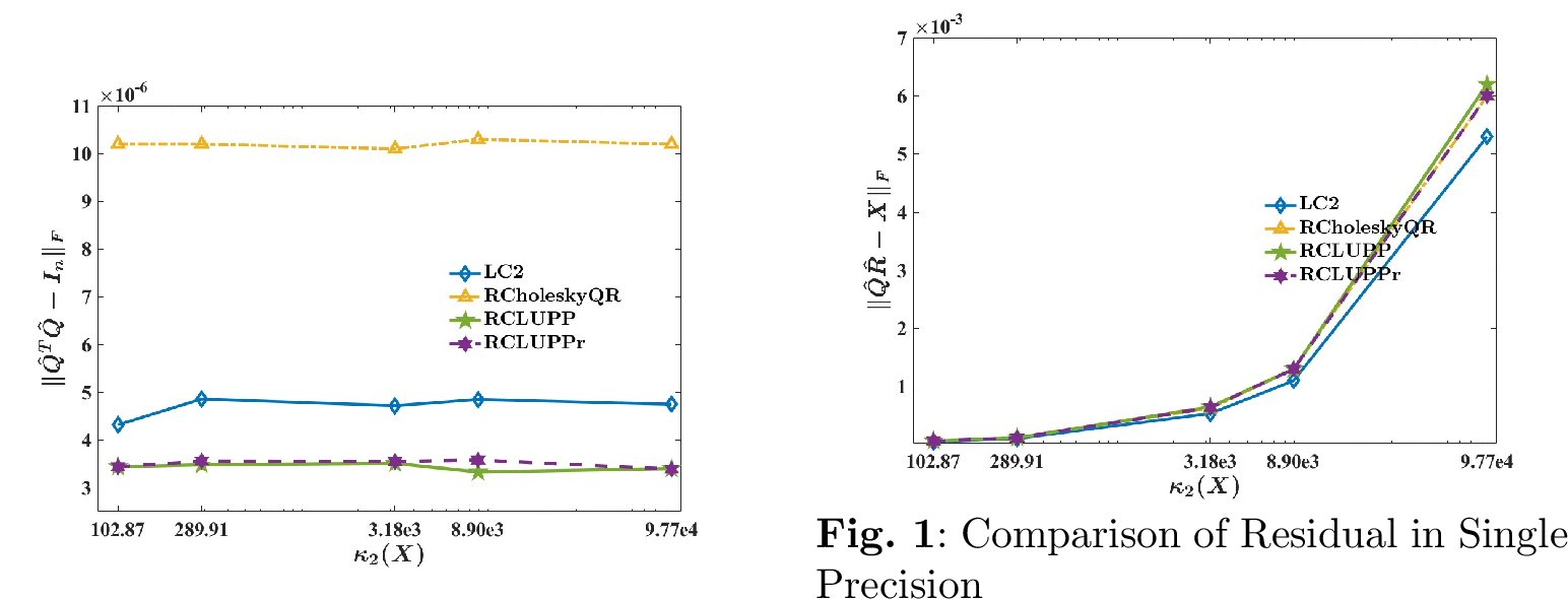
Figure 7 and Figure [fig:s2] show that RCLUPPr achieves numerical stability comparable to that of LC2 and RCLUPP in both orthogonality and residual in the single precision. Consistent with the findings in [11], RCLUPPr also exhibits superior orthogonality compared to that of RCholeskyQR across different precisions.
5.1.2 Double precision↩︎
Here, we consider the case of double precision with \({\boldsymbol{u}}_{b}={\boldsymbol{u}}=2^{-53}\) in Assumption 1. We take a numerical example of the Poisson-type electric-potential equation arising from a one-dimensional capacitively coupled plasma (1D-CCP) fluid simulation [21], [22]. In this example, the ill-conditioned matrix is extracted from the implicit finite-volume discretization of the electric-potential equation along the inter-electrode direction of a 1D-CCP discharge. The 1D-CCP configuration is closely related to the standard low-pressure capacitive-discharge benchmark settings in [21], while the implicit treatment of the charged-particle transport terms follows the common strategy used in the gas-discharge fluid simulations [22]. The electric-potential equation can be written in the following general form: \[-\frac{d}{dx}\left(\epsilon_{\mathrm{eff}}\frac{d\phi}{dx}\right)=\rho_{\mathrm{eff}}, \nonumber\] where \(\phi\) is the electric potential, and \(\epsilon_{\mathrm{eff}}\) and \(\rho_{\mathrm{eff}}\) denote the effective permittivity and the effective charge/source term introduced by the implicit coupling between Poisson’s equation and the charged-species transport equations. In the plasma region, \(\epsilon_{\mathrm{eff}}\) includes the contribution from the implicit electron drift term. \(\rho_{\mathrm{eff}}\) contains the ion, electron, and diffusion-related source terms. After the face-based finite-volume discretization, the equation for an interior control volume \(P\) can be written as \[a_P\phi_P+\sum_{N\in\mathcal{N}(P)}a_{PN}\phi_N=b_P, \nonumber\] with \[a_{PN}=-\frac{S_f}{d_{PN}}\bar{\epsilon}_f, \qquad \bar{\epsilon}_f=\frac{\epsilon_{\mathrm{eff},P}+\epsilon_{\mathrm{eff},N}}{2}, \qquad a_P=-\sum_{N\in\mathcal{N}(P)}a_{PN}. \nonumber\] Here, \(\mathcal{N}(P)\) denotes the neighboring control volumes of \(P\), \(S_f\) is the face area, \(d_{PN}\) is the distance between the centroids of \(P\) and its neighboring control volume \(N\), and \(\bar{\epsilon}_f\) is the face-interpolated effective permittivity. Therefore, the resulting linear system is \[A_{1}\phi=b. \nonumber\] In the real 1D-CCP case, we have \(A_{1} \in \mathbb{R}^{130\times 130}\) with \(\kappa_2(A_{1})=1.21 \times 10^{17}\). Such an \(A_{1}\) provides a challenging test case for QR-based linear solvers. To generate the tall skinny \(X\) with different \(\kappa_{2}(X)\) while preserving the structure of the plasma-discretization matrix, we consider \[X_{1}=A_{1}+l_{1}I_{n}. \nonumber\] We vary \(l_{1}\) from \(10^{-12}\), \(10^{-13}\), \(10^{-14}\), \(10^{-15}\) to \(10^{-16}\) to modify \(\kappa_2(X_{1})\). Similar to case of the single precision, we construct the testing matrix \(X \in \mathbb{R}^{1300\times 130}\) by stacking \(10\) copies of \(X_{1}\) vertically with \(s=2n=260\). Numerical results of this group of experiments are shown in Figure 8 and Figure [fig:d2].
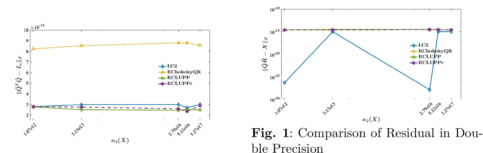
In the double precision, Figure 8 and Figure [fig:d2] show that RCLUPPr maintains excellent accuracy and numerical stability for the highly ill-conditioned \(X\). Combining these results with those in Figure 8 and Figure [fig:d2], we conclude that RCLUPPr is numerically stable in the uniform precision.
5.1.3 Mixed precision↩︎
We next examine the setting of the mixed precision as ‘single+double’ with \({\boldsymbol{u}}=2^{-24}\) and \({\boldsymbol{u}}_{b}=2^{-53}\) in Assumption 1. Following the same strategy as for RCLUPPr, we assign the double precision to all the steps except LUPP decomposition up to the computation of the \(Q\)-factor, \(W\), for LC2, RCholeskyQR and RCLUPP, while performing the remaining steps in the single precision. For RCLUPPr, we focus on two different cases, sRCLUPPr following Assumption 1 with LUPP decomposition in the single precision and dRCLUPPr with LUPP decomposition in the double precision.
Three numerical examples are used for the numerical stability and applicability of the algorithms, including the classical testing matrix based on the SVD, the arrowhead matrix and the ill-conditioned triangular matrix. The SVD-based testing matrix is a classical one for the test of numerical stability because of its convenience to alter \(\kappa_{2}(X)\). We fix \(m=2048\), \(n=64\) and \(s=2n=128\) for the algorithms. We build \(X\) as \[X=M \Sigma F^{T}, \nonumber\] with \(M \in \mathbb{R}^{2048\times 64}\) and \(F \in \mathbb{R}^{64\times 64}\) orthogonal and \[\Sigma = {\rm diag}(1, \sigma^{\frac{1}{63}}, \cdots, \sigma^{\frac{62}{63}}, \sigma) \in \mathbb{R}^{64\times 64}, \nonumber\] diagonal. Here, we can have \(\sigma_{1}(X)=\|X\|_{2}=1\), \(0<\sigma<1\) as \(\sigma_{n}(X)\). Therefore, we vary \(\sigma\) from \(10^{-2}\), \(10^{-4}\), \(10^{-6}\), \(10^{-8}\) and \(10^{-10}\) to change \(\kappa_{2}(X)\) for the algorithms. Numerical experiments of the SVD-based matrices are shown in Figure 9 and Figure [fig:mixs2].
The arrowhead matrix is widely used in the control theory and some eigenvalue problems, see [23]–[25] for more details. Many arrowhead matrices are very ill-conditioned and suitable for the test of the applicability of the algorithms. In this case, we fix \(m=20000\), \(n=50\) and \(s=2n=100\). We define \(v_{1}=(0,1,1, \cdots, 1,1)^{\top} \in \mathbb{R}^{50}\), \(v_{2}=(1,0,0, \cdots, 0,0)^{\top} \in \mathbb{R}^{20000}\) and \(E={\rm diag}(1, g^{\frac{1}{49}}, \cdots, g^{\frac{48}{49}}, g) \in \mathbb{R}^{50\times 50}\). Here, \(g\) is a positive constant that we can modify. We can construct \(X_{1} \in \mathbb{R}^{20000\times 50}\) as \[X_{1}= \begin{pmatrix} E \\ \mathbb{O} \nonumber \end{pmatrix}.\] Here, \(\mathbb{O}\) is the matrix with all the elements \(0\). Therefore, we can build \(X \in \mathbb{R}^{20000\times 50}\) as \[X=-5v_{2} \cdot v_{1}^{\top}+X_{1}. \nonumber\] For the arrowhead \(X\), we vary \(g\) from \(10^{-10}\), \(10^{-15}\), \(10^{-20}\), \(10^{-25}\) to \(10^{-30}\) to get \(X\) with different \(\kappa_{2}(X)\). Numerical results of the orthogonality and residual for the arrowhead \(X\) are shown in Figure 10 and Figure [fig:mixa2].
We also consider a class of \(X \in \mathbb{R}^{m\times n}\), where the \(L\) factor obtained from LUPP decomposition of \(X\) is very ill-conditioned. A representative construction \(X\) takes the form \[X = \begin{bmatrix} X_{u}+s_{u}I_{n} \\ X_{l} \end{bmatrix},\] where \(X_{u} \in \mathbb{R}^{n \times n}\) is an ill-conditioned lower-triangular matrix and \(X_{z} \in \mathbb{R}^{(m-n)\times n}\) is a zero block. All the elements on the diagonal of \(X_{u}\) are \(1\) and those under the diagonal \(-1\). This type of matrices appears in many real-world applications, including eigenvalue problems, control theory and the circuit simulation [13], [14], [26]. Here, we take \(m=4000\), \(n=100\) and \(s=2n=200\). We vary \(s_{u}\) from \(10^{-15}\), \(10^{-14}\), \(10^{-13}\), \(10^{-12}\) to \(10^{-11}\) to vary \(\kappa_{2}(X)\). Numerical experiments of such a type of matrices are shown in Figure 11 and Figure [fig:mixt2].
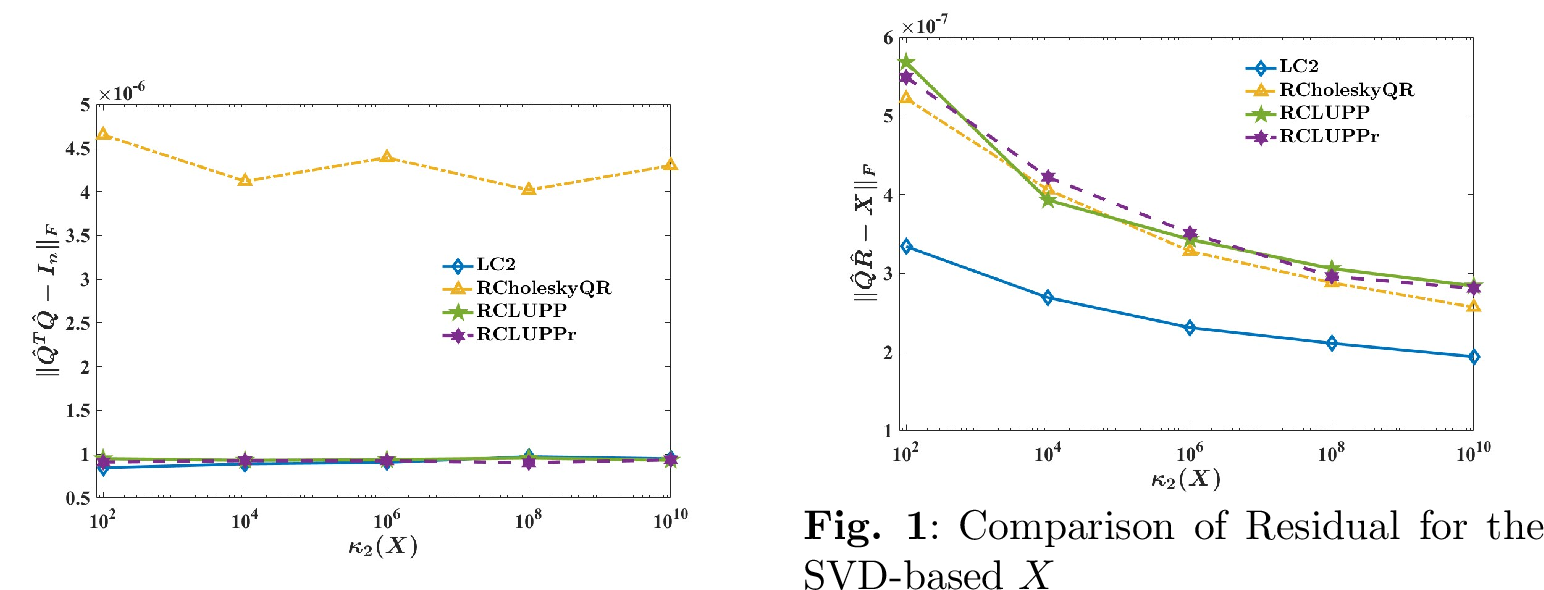
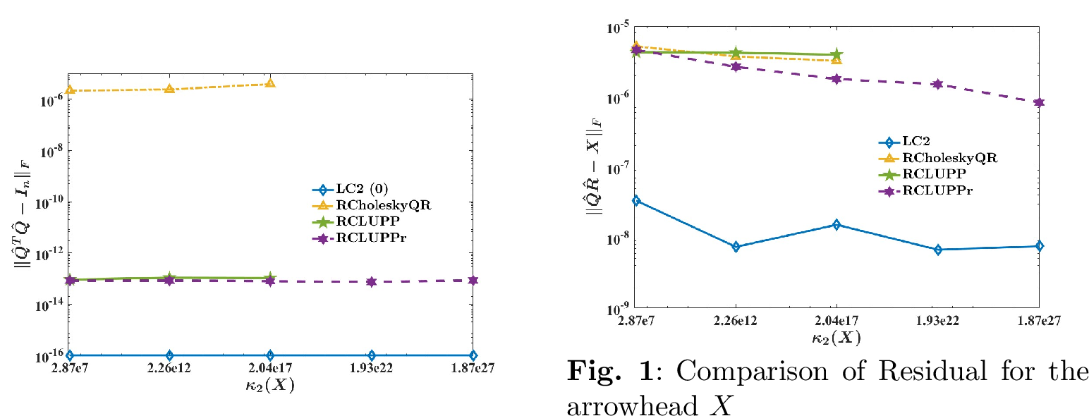
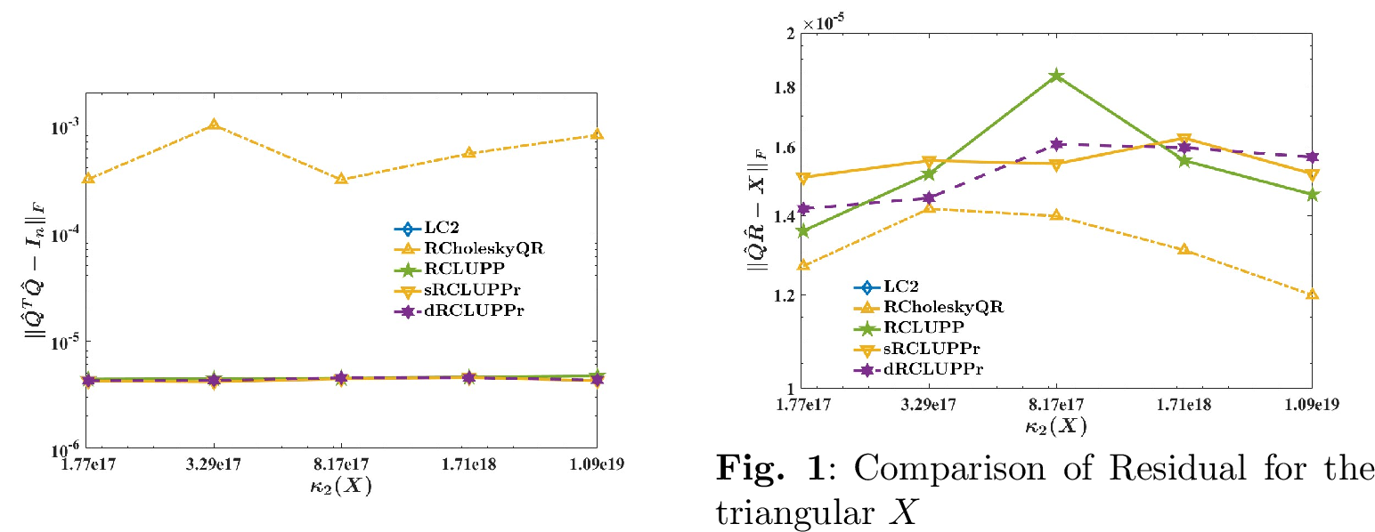
Figure 9 and Figure [fig:mixs2] show that RCLUPPr achieves accuracy and numerical stability comparable to those of LC2 and RCLUPP in the mixed-precision, consistent with the observations in [11] and Table 1. The advantage of the orthogonality for RCLUPPr over RCholeskyQR is also preserved. For the highly ill-conditioned matrices, Figure 10 and Figure [fig:mixa2] confirm that RCLUPPr retains superior applicability compared to RCholeskyQR, again in agreement with [11] and Table ¿tbl:tab:comparison1?. This shows the strong preconditioning effect of performing LUPP decomposition before matrix sketching is clearly evidenced by the excellent performance of both LC2 and RCLUPPr. Figure 11 and Figure [fig:mixt2] demonstrate the superior performance of RCLUPPr over LC2 when the \(L\)-factor obtained from LUPP decomposition is ill-conditioned. This observation aligns with the numerical results reported in [11] and the theoretical comparison in Table ¿tbl:tab:comparison2?. Regarding sRCLUPPr with LUPP decomposition in the single precision and dRCLUPPr with LUPP decomposition in the double-precision, the former frequently encounters numerical breakdown on the arrowhead matrix in the highly ill-conditioned cases. Although slightly slower, dRCLUPPr is considerably more stable and robust owing to the use of LUPP decomposition in the double precision LU preconditioning. The single precision offers significantly lower error tolerance than the double precision. Consequently, the rounding error introduced by LUPP is greatly amplified as shown in 38 40 , often leading to numerical breakdown in CholeskyQR2 afterwards. In contrast, the double precision provides a sufficient safety margin, enabling dRCLUPPr to maintain markedly superior robustness in the real cases. In practice, dRCLUPPr can be viewed as a safer and more reliable choice for the real-world experiments.
5.2 Tests of robustness of RCLUPPr↩︎
To thoroughly assess the robustness of RCLUPPr, we conduct two groups of experiments in the double precision: the well-conditioned and ill-conditioned cases. As far as we know, this is the first in the existing works of CholeskyQR. For the well-conditioned case, we employ the SVD-based matrix with \(m=2000\), \(n=50\), and \(\|X\|_{2}=1\). We vary \(\kappa_2(X)\) by changing \(\sigma_n\) from \(10^{-2}\), \(10^{-4}\), \(10^{-6}\), \(10^{-8}\) to \(10^{-10}\). We fix \(\epsilon=0.5\), \(p=0.6\) and \(s=2n=100\). We record the times of success and the rate of success for RCLUPPr in \(1000\) times, which are shown in Table 3. When \(\sigma=10^{-10}\), we vary \(s\) from \(50\), \(100\), \(200\), \(500\) to \(1000\) and exhibit the corresponding results in Table 4. For the ill-conditioned \(X\), we focus on the arrowhead matrices with \(m=20000\) and \(n=50\). \(\kappa_{2}(X)\) is controlled by varying the parameter \(g \in\{10^{-15},10^{-20},10^{-25},10^{-30},10^{-35}\}\). We vary \(s\) in the same manner as that in the well-conditioned cases. Numerical experiments are summarized in Table 5 and Table 6.
| \(\kappa_{2}(X)\) | \(1e+2\) | \(1e+4\) | \(1e+6\) | \(1e+8\) | \(1e+10\) |
|---|---|---|---|---|---|
| Times of success | \(1000\) | \(1000\) | \(1000\) | \(1000\) | \(1000\) |
| Rates of success | \(100\%\) | \(100\%\) | \(100\%\) | \(100\%\) | \(100\%\) |
| \(s\) | \(50\) | \(100\) | \(200\) | \(500\) | \(1000\) |
|---|---|---|---|---|---|
| Times of success | \(1000\) | \(1000\) | \(1000\) | \(1000\) | \(1000\) |
| Rates of success | \(100\%\) | \(100\%\) | \(100\%\) | \(100\%\) | \(100\%\) |
| \(\kappa_{2}(X)\) | \(2.04e+17\) | \(1.93e+22\) | \(1.87e+27\) | \(1.84e+32\) | \(1.82e+37\) |
|---|---|---|---|---|---|
| Times of success | \(1000\) | \(1000\) | \(773\) | \(761\) | \(764\) |
| Rates of success | \(100\%\) | \(100\%\) | \(77.3\%\) | \(76.1\%\) | \(76.4\%\) |
| \(s\) | \(50\) | \(100\) | \(200\) | \(500\) | \(1000\) |
|---|---|---|---|---|---|
| Times of success | \(779\) | \(764\) | \(750\) | \(766\) | \(749\) |
| Rates of success | \(77.9\%\) | \(76.4\%\) | \(75.0\%\) | \(76.6\%\) | \(74.9\%\) |
Table 3 and Table 4 demonstrate that RCLUPPr is highly robust in the well-conditioned cases, maintaining numerical stability across thousands of independent trials. For the severely ill-conditioned matrices, Table 5 shows that numerical breakdown may occur when \(\kappa_2(X)\) becomes sufficiently large. Nevertheless, RCLUPPr still achieves a success rate of approximately \(75\%\), which substantially exceeds the theoretical lower bound of probability \(1-p=0.4\) guaranteed by Definition 2 and Theorem 1. Table 6 further indicates that the choice of \(s\) for the Gaussian sketch has negligible impact on the robustness in the ill-conditioned regime. Consequently, a small \(s=\mathcal{O}(n)\), or even \(s=n\), can be safely adopted to improve the efficiency of RCLUPPr without sacrificing the reliability.
5.3 Accelerating RCLUPPr in the double precision↩︎
In this part, we discuss some practical acceleration strategies for RCLUPPr in the double precision. As shown in [11], although RCLUPPr offers superior applicability and accuracy, its computational efficiency lags behind other CholeskyQR-type algorithms. Here, we introduce several targeted optimizations that significantly improve the CPU time (s) while fully preserving the numerical advantages of RCLUPPr.
5.3.1 Multi-sketching↩︎
For \(X \in \mathbb{R}^{m\times n}\), we can use the technique of multi-sketching in [10], [27] to replace a single Gaussian sketch. We can use a step of the CountSketch [16] before the Gaussian sketch to reduce the computational complexity of matrix sketching. When \(\Omega_{1} \in \mathbb{R}^{s_{1}\times m}\) is the sketch matrix of the CountSketch with \(s_{1} \le m\), according to [17], [28], \(s_{1}\) satisfies \[s \ge \frac{n^{2}+n}{\epsilon^{2}p}. \label{eq:multi}\tag{85}\] With \(\Omega \in \mathbb{R}^{s\times s_{1}}\) as the sketch matrix of the Gaussian sketch satisfying \(n \le s \le s_{1} \le m\), the comparison between the computational complexity of different types of sketching is shown in Table 7.
Table 7 indicates that multi-sketching becomes cheaper than the single Gaussian sketching when \(s(m-s_{1}) \ge m\). For the typical choice \(s=\mathcal{O}(n)\) for the Gaussian sketch, 85 yields the sufficient condition \[\frac{n^{2}+n}{\epsilon^{2}p} \le m-\mathcal{O}(\frac{m}{n}), \label{eq:multie}\tag{86}\] which is satisfied whenever \(m=an^{2}\) for a positive constant \(a\). Accordingly, we retain \(\epsilon=0.5\) and \(p=0.6\) in the experiments. We generate a test matrix \(X\in\mathbb{R}^{20000\times 20}\) using \(rand\) in MATLAB and fix \(s_{1}\) for the CountSketch as \(s_{1}=2800\). Varying \(s\) for the Gaussian sketch, we compare the CPU time (s) of RCLUPPr with and without multi-sketching. The results are summarized in Table 8. The table clearly demonstrates the effectiveness of multi-sketching in reducing the CPU time (s) once 86 still holds. As \(s\) increases, RCLUPPr with multi-sketching exhibits a substantial speed advantage over the case with the single Gaussian sketch, which is consistent with the analysis of computational complexity in Table 7. The rounding error analysis of RCLUPPr with multi-sketching can be taken following the same lines as in [10].
| \(Type of sketching\) | \(Computational complexity\) |
|---|---|
| \(Single-sketching\) | \(\mathcal{O}(smn)\) |
| \(Multi-sketching\) | \(\mathcal{O}(mn+ss_{1}n)\) |
| \(s\) | \(100\) | \(200\) | \(400\) | \(800\) | \(1600\) |
|---|---|---|---|---|---|
| Single-sketching | \(0.0432\) | \(0.0456\) | \(0.0492\) | \(0.0593\) | \(0.0802\) |
| Multi-sketching | \(0.0425\) | \(0.0431\) | \(0.0453\) | \(0.0455\) | \(0.0463\) |
| Reduction of the CPU time | \(1.7\%\) | \(5.8\%\) | \(8.6\%\) | \(30.3\%\) | \(42.3\%\) |
5.3.2 Adaptive RCLUPPr↩︎
We also investigate practical variants of RCLUPPr to further improve the efficiency. RCLUPPr with multi-sketching remains applicable for \(X\in\mathbb{R}^{m\times n}\) whenever \(m=\mathcal{O}(n^2)\), see 86 . Here, we consider performing LU decomposition without partial pivoting, which is significantly faster in many cases. Replacing the line \([L,U,P]=\mathrm{LU}(X)\) with \([L,U]=\mathrm{LU}(X)\) in Algorithm 6 yields the variant RCLUr, see Algorithm 12. To combine the high robustness of RCLUPPr with the speed of RCLUr, we propose an adaptive strategy called Adaptive RCLUPPr in Algorithm 13). It attempts the faster RCLUr in the beginning. Only upon detecting numerical breakdown (NaN/Inf) or when the tolerances of the orthogonality and residual are violated does it fall back to RCLUPPr. This hybrid approach achieves near-optimal runtime for the well-conditioned matrices while automatically guaranteeing the robustness for the ill-conditioned cases without requiring prior knowledge of the matrix properties.
For the numerical experiments, we use the SVD-based matrix with \(m=2000\), \(n=50\), \(\|X\|_{2}=1\) and \(\kappa_{2}(X)=10^{16}\). We set \(\tau_{ortho}=\tau_{res}=10^{-15}\). Table 9 compares the CPU time (s) of RCLUPPr and Adaptive RCLUPPr in this example. We find that Adaptive RCLUPPr is substantially faster than RCLUPPr, illustrating that it is a practical and efficient option for many ill-conditioned problems.
![Figure 12: [Q,R]=RCLUr(X)](/article/2607.15561/_pdflatex/vyujnxpo.png "fig:")

| \(s\) | \(50\) | \(100\) | \(200\) | \(400\) | \(800\) |
|---|---|---|---|---|---|
| RCLUPPr | \(0.0065\) | \(0.0074\) | \(0.0084\) | \(0.0093\) | \(0.0112\) |
| Adaptive RCLUPPr | \(0.0032\) | \(0.0038\) | \(0.0048\) | \(0.0059\) | \(0.0063\) |
| Reduction of the CPU time | \(50.8\%\) | \(48.6\%\) | \(42.9\%\) | \(36.7\%\) | \(43.8\%\) |
6 Conclusions↩︎
This work provides the first comprehensive rounding error analysis of RCLUPPr, a novel randomized CholeskyQR-type algorithm with direct LUPP decomposition. We rigorously prove that performing LUPP decomposition before matrix sketching yields better applicability compared to the existing algorithms. The algorithm is shown to be numerically stable and accurate across the single, double and the mixed-precision arithmetic. We further demonstrate its robustness through extensive experiments on the matrices from the real-world problems. Some practical strategies for accelerating RCLUPPr, including multi-sketching and Adaptive RCLUPPr based on LUPP decomposition, significantly improve the CPU time (s) while preserving all the theoretical advantages in the real implementations. Numerical results on the matrices from the optimal control, capacitively coupled plasma simulations, and the control theory confirm the effectiveness and practicality of RCLUPPr.
7 Acknowledgement↩︎
The authors declare that they have no conflict of interest. The dagger symbol (†) denotes the co-first authors. Haoran Guan and Zhenyu Zou are the co-first authors of this article. We express our great attitude to Professor Zhonghua Qiao from the Hong Kong Polytechnic University for his kind support and help. We would like to thank Mr. Yuan Liang from Beijing Normal University, Zhuhai, for his valuable suggestions and examples related to the numerical experiments. Additionally, we appreciate the discussions with Professor Valeria Simoncini from University of Bologna and Professor Michael Kwok-Po Ng from Hong Kong Baptist University regarding CholeskyQR and randomized linear algebra, especially matrix sketching.
Data availability↩︎
The authors declare that all data supporting the findings of this study are available within this article.