On the Role of Normalization in Binary Iterative Hard Thresholding for 1-bit Compressed Sensing
July 17, 2026
Abstract
Binary Iterative Hard Thresholding (BIHT) is a simple, yet effective, greedy method for recovering a sparse vector from one-bit sign measurements. In its original form, BIHT performs a “gradient-descent” step, followed by hard thresholding. A convergence analysis of this algorithm was left open in the introductory work of [1] and has remained unresolved for over a decade, with subsequent sharp analyses studying a normalized variant instead, that additionally projects every iterate onto the unit sphere. This paper resolves that gap and characterizes when per-iteration normalization is algorithmically necessary.
In the noiseless setting, we prove a universal, sample-optimal convergence theorem for the original BIHT algorithm. Specifically, with \(\widetilde{O}\parens *{s/\epsilon}\) measurements, a deterministic finite-time iterate has directional error at most \(\epsilon\), simultaneously for every \(s\)-sparse unit vector. This matches the optimal sample dependence achieved by normalized BIHT in prior work. Thus, in the noiseless regime, per-iterate normalization is unnecessary for optimal recovery.
Under sign corruptions, we prove a sharp separation. If at most a \(\tau\) fraction of signs are flipped adversarially, then BIHT, without per-iterate normalization, still reaches the robust error floor at an early iterate with a matching \(\widetilde{O}\parens *{s/\epsilon}\) sample complexity rate as its normalized variant. This recovery, however, is not stable. We prove a scalar lower bound showing that any nontrivial corruption pattern, even one that involves only one flipped sign together with one clean sign, forces the iterates to oscillate indefinitely. Consequently, no general last-iterate convergence theorem can hold for BIHT under sign corruptions, while its normalized surrogate provably escapes this instance.
1 Introduction↩︎
In one-bit compressed sensing, a high-dimensional signal is observed only through the signs of linear measurements. Given a sensing matrix \(A \in \mathbb{R}^{m \times n}\) and an unknown \(s\)-sparse signal \(x^\star\in\Sigma_s^n\cap\mathcal{S}^{n-1}\), where \(\Sigma_s^n \triangleq\set{x\in\R^n \given \norm{x}_0 \le s}\), the vector of \(m\) observations is \[\begin{align} y = \sign(A x^\star) \in \{\pm 1\}^m, \end{align}\] one bit per measurement. This model, first introduced in the work of [2], sits at the extreme end of quantization, discarding all magnitude information. Since signs are invariant under positive rescaling of the signal \(x^\star\), the only identifiable component is the direction, and the target is normalized to the sparse unit sphere without any loss of generality. The objective is to produce, from as few measurements as possible, a directional estimate \(\widehat{x}\) that is \(\epsilon\)-close to \(x^\star\) in \(\ell_2\) distance. If the sensing matrix has standard Gaussian rows, then \(m = \widetilde{\Theta}\parens*{s/\epsilon}\) measurements are necessary and sufficient [1], while the first computationally tractable algorithm via convex programming required \(m = \widetilde{\Theta}\parens*{s/\epsilon^5}\) measurements [3].
Let \(\mathcal{T}_s(v)\) denote all \(s\)-term hard-thresholdings of \(v\), with arbitrary tie-breaking
Set \(\eta = \sqrt{2\pi}\)
[1] proposed Binary Iterative Hard Thresholding (BIHT) ([alg:biht]) as a simple first-order method for this problem, analogous to the iterative hard thresholding algorithm for compressed sensing [4]. Starting from a sparse unit vector, BIHT iterates a sign-mismatch correction, interpretable as a subgradient descent step on a one-sided sign-consistency objective, followed by hard thresholding onto the set of \(s\)-sparse vectors, with a single normalization applied to the final output. The algorithm is simple to implement, requires no tuning beyond the sparsity level, and has remained the standard first-order baseline for one-bit recovery. A convergence analysis of BIHT was left open in [1], and has remained unresolved for over a decade.
Early progress toward a convergence theory for BIHT focused largely on one-step analyses. [5] showed that the first iterate of BIHT achieves error \(\epsilon\) from \(m = \widetilde{O}\parens*{s/\epsilon^2}\) measurements; similar one-step guarantees appear in [6]. Beyond the first iterate, however, these analyses do not track the BIHT trajectory, and their dependence on \(\epsilon\) is quadratically suboptimal. [7] then studied the full trajectory, interpreting BIHT as a projected subgradient method under sparsity constraints, and proved that the subsequent iterates remain bounded, retaining the accuracy of the first step. This yields stability of the trajectory, but no reduction of the error beyond the first iteration. A convergence theorem for the algorithm of [1], one in which the iterates provably improve, remained out of reach.
Sharp guarantees were finally obtained by changing the algorithm. [8] and [9]–[11] analyze a normalized variant of BIHT that additionally projects every iterate onto the unit sphere. Normalizing the iterates allows one to translate a so-called restricted approximate invertibility condition (RAIC) of Gaussian random matrices to show contraction of the estimation error at every step. For the normalized variant of BIHT with Gaussian sensing matrices, the theory is, by now, essentially complete: [9] proves universal recovery with the optimal \(\widetilde{O}\parens *{s/\epsilon}\) measurements, and [10] extends the guarantee to adversarial sign corruptions with a matching robust error floor. In each of these analyses, per-iterate normalization is crucial: since the RAIC holds uniformly for any pair of sparse vectors, contraction is guaranteed whenever the iterates are on the unit sphere. The original algorithm offers no such control over the iterates, and its analysis has remained open.
This paper resolves that open question, and in doing so, characterizes exactly when per-iteration normalization is algorithmically necessary: never in the noiseless regime, and in a precise, last-iterate sense, always under corruption.
1.1 Our Results↩︎
1.1.0.1 Normalization is unnecessary without noise.
Our first result is a universal, sample-optimal convergence theorem for the original, normalization-free BIHT algorithm under noiseless measurements.
Theorem 1 (Informal version of 4). Let \(0 < \epsilon \le 1/64\) and let \(A\in \R^{m\times n}\) have independent standard Gaussian entries. If \(m = \widetilde{O}(s/\epsilon)\), then with high probability over the draw of \(A\), the following holds simultaneously for every \(x^\star \in \Sigma^n_s \cap \mathcal{S}^{n-1}\), every sparse unit initialization, and every sequence of hard-thresholding tie-breaks: BIHT, without per-iterate normalization, run for \(T = O\parens{\log\parens{1/\epsilon}}\) iterations on \(y = \sign\parens{Ax^\star}\), returns an estimate \(\widehat{x}_{\mathrm{BIHT}}\) with \(\norm{\widehat{x}_{\mathrm{BIHT}} - x^\star}_2 \le \epsilon\).
The sample complexity matches the optimal dependence achieved by normalized BIHT [9], and the guarantee is of the same universal form: a single draw of the sensing matrix serves all sparse targets simultaneously. Moreover, the guarantee is a last-iterate statement at a deterministic, \(\epsilon\)-computable horizon. Therefore, in the noiseless regime, [alg:biht], as proposed in [1], is sample-optimal, and per-iterate normalization is unnecessary.
1.1.0.2 Under corruption, the optimum cannot be held…
Our second result concerns sign corruptions, where the observed labels \(y\) may differ from \(\sign(Ax^\star)\) in up to a \(\tau\) fraction of coordinates. We find that a single corrupted measurement already negates the feasibility of last-iterate convergence for the fixed-step dynamics, even in dimension one.
Theorem 2 (Informal version of 5). Let \(n = s = 1\) and let \(A\) have independent standard Gaussian entries. For every corruption pattern that flips at least one sign and leaves at least one sign clean, and every fixed nonzero initialization independent of \(A\), the normalization-free fixed-step iterates almost surely change sign infinitely often. Consequently, \[\limsup_{t \to \infty} \norm*{ \frac{x^{(t)}}{\abs{x^{(t)}}} - x^\star }_2 = 2.\]
That is, the directional error returns to its maximum possible value infinitely often, even when a single corrupted bit lies within otherwise clean measurements. Since the guarantee being ruled out is uniform over dimensions, sparsity levels, targets, and corruption patterns, this single scalar instance suffices to demonstrate impossibility. On the same instance, if there are more clean bits than flipped ones, normalized BIHT recovers the correct sign from the first step onward, except with exponentially small probability (4.2.1.1).
1.1.0.3 …but it is reached, and one can certify when.
In light of 5, a hitting-time guarantee is the strongest form of convergence available to the fixed-step dynamics. Our third result shows that BIHT, without per-iterate normalization, achieves it at the optimal accuracy scale. Our results are stated for the robust error floor \[\gamma(\epsilon, \tau) \triangleq \epsilon + c_1\sqrt{\epsilon\tau} + c_2\, \tau\sqrt{\log(2e/\tau)},\] which is the same floor attained by normalized BIHT in this model [10].
Theorem 3 (Informal version of 6). Under the same measurement budget as 1, the following holds simultaneously with high probability for every sparse unit target, every admissible corruption pattern, and every sparse unit initialization: if \(\gamma\parens{\epsilon,\tau} \le 1/64\), then some iterate \(t_{\mathrm{hit}} \le O\parens{\log\parens{1/\gamma\parens{\epsilon,\tau}}}\) of normalization-free BIHT satisfies \[\begin{align} \norm*{\frac{x^{t_{\mathrm{hit}}}}{\norm{x^{t_{\mathrm{hit}}}}_2} - x^\star}_2 \le \gamma\parens{\epsilon, \tau}, \end{align}\] and every iterate up to \(t_{\mathrm{hit}}\) is nonzero with norm within \(1/64\) of one.
The trajectory is generated without knowledge of \(\tau\), but the certificate identifying the relevant accuracy scale is \(\tau\)-dependent. 6 is therefore a hitting-time guarantee, and, by 5, necessarily so. When an a-priori corruption budget \(\tau \le \tau_0\) is available, the guarantee upgrades: running normalization-free BIHT for a fixed horizon \(T_0 = O(\log(1/\gamma\parens{\epsilon,\tau_0}))\) returns an estimate within the worst-case floor \(\gamma\parens{\epsilon, \tau_0}\) (1), and the accuracy persists for a window of \(\Omega(1/\gamma(\epsilon,\tau_0))\) subsequent iterations, so the stopping time is stable to timing errors (2). Together, Theorems 5 and 6 explain an interesting empirical phenomenon that appears in [11] . They observe that, without normalization, the BIHT error curve first drops to a robust floor and then oscillates around a constant error. 6 explains the drop, and 5 explains the oscillation ( 1 (b)).
2 Preliminaries↩︎
2.1 Notation↩︎
For \(s\in[n]\), \(\Sigma_s^n\triangleq\set{x\in\R^n\given \norm{x}_0\le s}\) denotes the set of \(s\)-sparse vectors in \(\R^n\). We write \(\mathcal{S}^{n-1}\) for the Euclidean unit sphere and use \(x^\star\) for the unknown sparse unit vector. The sign function is defined by \(\sign(t)=1\) for \(t\ge0\) and \(\sign(t)=-1\) otherwise, and is applied coordinate-wise to vectors. For \(U\subseteq[n]\), \(\mathcal{T}_U\) denotes coordinate restriction to the set \(U\). For \(v\in\R^n\), \(\mathcal{T}_s(v)\) denotes the set of Euclidean projections of \(v\) onto \(\Sigma_s^n\). Equivalently, \(\mathcal{T}_s(v)\) is the set of all hard-thresholded vectors obtained by retaining any \(s\) largest coordinates of \(v\) in magnitude and zeroing out the rest, with arbitrary tie-breaking. We write \(x\in\mathcal{T}_s(v)\) when \(x\) is any such valid hard-thresholded output. Throughout, \(\eta=\sqrt{2\pi}\) denotes the fixed BIHT step-size and \(A\in R^{m\times n}\) denotes the sensing matrix. We use \(\gtrsim\) to denote \(\ge\) upto universal constants.
Under noiseless measurements, \(y = \sign(Ax^\star)\). We use the following notation for the correction term of [alg:biht] \[\begin{align} \label{eq:hA-def} h_A(p,q) \triangleq \frac{\eta}{m}A^\top\cdot\frac{1}{2} \parens*{\sign(Ap)-\sign(Aq)}, \end{align}\tag{1}\] for \(p,q \in \R^n.\) For a set \(J\subseteq[n]\), we use \(h_{A;J}\) to denote the correction term restricted to the supports of the variables it applies to, and the coordinates in \(J\). Formally, \[\begin{align} h_{A;J}(p,q) \triangleq \mathcal{T}_{\supp(p)\cup\supp(q)\cup J} \parens*{h_A(p,q)} \end{align}\] The role of the restriction is to match the coordinates that can affect a hard-thresholded update. In our proofs, the set \(J\) usually often be selected by the next hard-thresholding step, and is therefore data-dependent.
Under measurements corrupted by adversarial noise, the observation vector \(y\in\braces *{\pm 1}^m\) satisfies \(d_H(y, \sign(Ax^\star))\le \tau m\), where \(d_H\parens *{\cdot}\) denotes the Hamming distance. For a fixed matrix \(A\) and corruption level \(\tau\in[0,1]\), let \[\begin{align} \mathcal{F}_A(\tau)\triangleq\set*{f:\R^n\to\set{\pm1}^m\given d_{\mathrm H}(f(z),\sign(Az))\le \tau m\text{ for every }z\in\R^n}. \end{align}\] The set \(\mathcal{F}_A(\tau)\) comprises of all possible ways an adversary can corrupt the clean measurements, given they are only allowed to change \(\tau\) fraction of the data. We will need to then modify the correction term in 1 to measure the mismatch between the corrupted measurements and the current iterate signs. Formally, for every corruption pattern \(f\in\mathcal{F}_A(\tau)\), define \[\begin{align} h_{f;A}(p,q) \triangleq \frac{\eta}{m}A^\top\cdot\frac{1}{2} \parens*{f(p)-\sign(Aq)} \end{align}\] and, for \(J\subseteq[n]\), \[\begin{align} h_{f;A;J}(p,q) \triangleq \mathcal{T}_{\supp(p)\cup\supp(q)\cup J} \parens*{h_{f;A}(p,q)}. \end{align}\] As before, the support restriction ensures that the analysis matches the coordinates that can meaningfully affect the hard-thresholded updates, and involves data-dependent coordinates.
2.2 Deterministic Tools↩︎
We first record two elementary facts about hard thresholding.
Lemma 1 (Hard thresholding is a two-approximate projector). Let \(v\in\R^n\), \(w\in\mathcal{T}_s(v)\), and let \(z\in\Sigma_s^n\). Then, \[\begin{align} \norm{w-z}_2 \le 2\norm{v-z}_2 \end{align}\]
Proof. Since \(w\) is a closest \(s\)-sparse vector to \(v\), we have \(\norm{v-w}_2\le\norm{v-z}_2\). The claim follows by the triangle inequality. ◻
Lemma 2 (Restricting to a support containing the selected output). Let \(v\in\R^n\), let \(z\in\mathcal{T}_s(v)\), and let \(U\subseteq[n]\) satisfy \(\supp(z)\subseteq U\). Then \(z\in\mathcal{T}_s(\mathcal{T}_U(v))\).
Proof. Let \(I=\supp(z)\). Since \(z\) is a valid hard-thresholded output of \(v\), the support \(I\) captures at least as much squared mass of \(v\) as any other support of size at most \(s\). Restricting to a set \(U\) that contains \(I\) leaves the mass on \(I\) unchanged and cannot improve any support outside \(U\). Thus \(I\) remains an optimal hard-thresholding support after restriction. ◻
The following fact is specific to one-bit measurements.
Lemma 3 (The sign correction only sees direction). Let \(z\neq0\) and set \(u=z/\norm{z}_2\). Then, for every \(p\in\R^n\), \(h_A(p,z)=h_A(p,u)\). Moreover, for every \(J\subseteq[n]\), \(h_{A;J}(p,z)=h_{A;J}(p,u)\). The same statement holds for \(h_{f;A}\) and \(h_{f;A;J}\) for every \(f\in\mathcal{F}_A(\tau)\).
Proof. Since \(z=\norm{z}_2u\) with \(\norm{z}_2>0\), positive rescaling preserves every coordinate of \(\sign(Az)\), including zero coordinates. Furthermore, \(z\) and \(u\) have the same support. ◻
Finally, we record the following elementary geometric fact: a non-unit vector that is close to a positive multiple of \(x\in \mathcal{S}^{n-1}\) is close to \(x\) after normalization.
Lemma 4 (Normalization around a radial target). Let \(x\in \mathcal{S}^{n-1}\), let \(\alpha>0\), and let \(z\in\R^n\) satisfy \(\norm{z-\alpha x}_2\le \alpha/2\). Then \(z\neq0\), and \[\begin{align} \norm*{\frac{z}{\norm{z}_2}-x}_2 \le \frac{4}{\alpha}\norm{z-\alpha x}_2 \end{align}\]
Proof. Write \(z=\alpha x+\nu\). The assumption gives \(\norm{z}_2\ge\alpha/2\). Comparing \(z/\norm{z}_2\) first to \(\alpha x/\norm{z}_2\), and then using \(\abs{\norm{z}_2-\alpha}\le\norm{\nu}_2\), gives the claim. ◻
2.3 Random Matrix Tools↩︎
Definition 1 (Restricted approximate invertibility condition). Let \(c_1,c_2,\delta>0\). We say that \(A\) satisfies \((s,n,\delta,c_1,c_2)\)-RAIC if, for every \(p,q\in\Sigma_s^n\cap S^{n-1}\) and every \(J\subseteq[n]\) with \(\card J\le s\), \[\begin{align} \norm{(p-q)-h_{A;J}(p,q)}_2 \le c_1\sqrt{\delta\norm{p-q}_2} + c_2\delta \end{align}\]
There exist absolute constants \(c_1,c_2>0\) such that the following holds. Let \(1\le s\le n\), \(0<\delta<1\), and \(0<\rho<1\). Let \(A\in\R^{m\times n}\) have independent \(\mathcal{N}(0,I_n)\) rows. If \[\begin{align} m \gtrsim \frac{s}{\delta}\log\parens*{\frac{en}{s}} \sqrt{\log\parens*{\frac{2e}{\delta}}} + \frac{s}{\delta}\log^{3/2}\parens*{\frac{2e}{\delta}} + \frac{1}{\delta}\log\parens*{\frac{1}{\rho}} \sqrt{\log\parens*{\frac{2e}{\delta}}} \end{align}\] then \(A\) satisfies \((s,n,\delta,c_1,c_2)\)-RAIC with probability at least \(1-\rho\).
There exist absolute constants \(b_1, b_2, b_3, b_4 > 0\) such that the following holds. Let \(1 \le s \le n\), \(0 < \delta < 1\), \(0 < \rho < 1\), and \(0 \le \tau \le 1\). Let \(A \in \mathbb{R}^{m \times n}\) have independent \(\mathcal{N}(0, I_n)\) rows. If \[\begin{align} m \gtrsim \frac{s}{\delta} \log\parens*{\frac{en}{s}} \sqrt{\log\parens*{\frac{2e}{\delta}}} + \frac{s}{\delta} \log^{3/2}\parens*{\frac{2e}{\delta}} + \frac{1}{\delta} \log\parens*{\frac{1}{\rho}} \sqrt{\log\parens*{\frac{2e}{\delta}}} \end{align}\] then, with probability at least \(1 - \rho\), the following holds simultaneously for every \(f \in \mathcal{F}_A(\tau)\), every \(p, q \in \Sigma_s^n \cap S^{n-1}\), and every \(J \subseteq [n]\) with \(\abs{J} \le s\): \[\begin{align} \norm*{(p - q) - h_{f;A;J}(p, q)}_2 \le b_1 \sqrt{\delta \norm{p - q}_2} + b_2 \delta + b_3 \sqrt{\delta \tau} + b_4 \tau \sqrt{\log\parens*{\frac{2e}{\tau}}}, \end{align}\] with the convention that \(\tau\sqrt{\log(2e/\tau)} = 0\) when \(\tau = 0\).
3 Overview of Techniques↩︎
3.0.0.1 Population geometry.
Our proofs crucially depend on the geometric structure of the problem. We will first isolate the behavior of the iterates at the population level. Consider noiseless measurements \(y=\sign(Ax^\star)\) where \(A\) has standard Gaussian rows \(\parens*{a_1, \cdots , a_m}\), and a direction \(u\in \mathcal{S}^{n-1}\). By rotational invariance of the Gaussian distribution, \[\begin{align} \E_{a\sim \mathcal{N}(0,I_n)}{a\operatorname{sign}(\dotprod{a,u})} = \sqrt{\frac{2}{\pi}}u \end{align}\] Consequently, for unit vectors \(p,q\in\mathcal{S}^{n-1}\), \[\begin{align} \label{eq:population-correction} \E *{\frac{\sqrt{2\pi}}{2}a\parens{\operatorname{sign}(\dotprod{a,p})-\operatorname{sign}(\dotprod{a,q})}} = p-q. \end{align}\tag{2}\] The random vector inside the expectation is precisely the single-measurement contribution to the BIHT correction \(h_A(p,q)\) in 1 ; indeed, for fixed \(p,q\), the empirical correction \(h_A(p,q)\) is the average of these contributions over the rows of \(A\).
Consider the corresponding population dynamics, in which the empirical correction is replaced by its expectation over a row of \(A\) and the current state is held fixed. If the fixed state \(z\) is a unit vector, then 2 applies to the pair \((x^\star,z)\), and the population pre-threshold update is \[\begin{align} z+\E{h_A(x^\star,z)} = z+(x^\star-z) = x^\star \end{align}\] We often refer to this pre-threshold vector, and its empirical counterpart, as the "dense" iterate. Observe that, prior to thresholding, the update is exactly aligned with the target when \(z\in \mathcal{S}^{n-1}\). Therefore, keeping every iterate on the unit sphere makes the population dynamics nearly tautological: each correction points exactly from the current iterate to the target. Hard thresholding does not disrupt this geometry. Indeed, if the dense vector is close to \(x^\star\), then every hard-thresholded output is also close to \(x^\star\) up to constant factors, since \(x^\star\in\Sigma_s^n\) is a valid comparison point for projection onto \(\Sigma_s^n\) (see 1).
Without normalization, the population dynamics does not enjoy this property. If \(z\neq 0\), we write \[\begin{align} z= r u \end{align}\] where the norm \(r = \norm{z}_2\) is not necessarily unit, and \(u = z/\norm{z}_2\) represents the direction. Since the sign function itself is norm invariant, so is the signed correction term, and \[\begin{align} h_A(x^\star,z)=h_A(x^\star,u) \end{align}\] Substituting the above in 2 implies that the population correction \(\E{h_A\parens *{x^\star, z}}\) still estimates \(x^\star- u\), and not \(x^\star-z\). Without per-iterate normalization, the dense next iterate is therefore \[\begin{align} \label{eq:unnormalized-old-pop-error} z+\E{h_A(x^\star,z)} = ru +x^\star-u = x^\star+(r-1)u \end{align}\tag{3}\] If the above dense iterate is compared against \(x^\star\), the term \((r-1)u\) appears as an additional, uncontrolled radial error that the normalized variant avoids by forcing \(r= 1\).
We argue that this comparison is the wrong one. Without normalization, the update should not be compared to \(x^\star\) but to \(r x^\star\) instead, i.e., the vector along the target direction, but with the current norm. Rewriting the unnormalized population update as \[\begin{align} \label{eq:unnormalized-new-pop-error} r {u}+x^\star-u &= r x^\star+(r-1)({u}-x^\star) \end{align}\tag{4}\] makes this phenomenon apparent. When compared against \(r x^\star\), the radial error no longer appears as the additive error in 3 . Together with the directional component, it gives the combined per-iterate error \((r-1)({u}-x^\star)\). This is indeed the right geometry for one-bit recovery, since an error that is purely radial should not meaningfully hurt the final answer. If the current state has the right direction, with \(u = x^\star\), then the vector \(z=r x^\star\) is already perfectly recovered after the final normalization, for every \(r>0\). An analysis that insists on controlling \(\norm{z - x^\star}_2\) penalizes the algorithm for failing to learn a scale that the measurements never contained in the first place.
Moreover, since the radial discrepancy only appears as \(\abs{r-1}\norm{u-x^\star}_2\), as long as the norm remains in a constant-sized window around \(1\), the population error around the moving reference is controlled by the current directional error. As a result, our proof makes no attempt to show that the norms of the iterates converge to one. Given the extreme quantization of the measurements, such a statement would be unnatural: sign measurements carry no radial information, and the iterates have no apparent reason to prefer unit-scale representatives of the target direction. What we need is strictly weaker: the norm must not drift out of this window during the finitely many iterations needed to recover the direction.
Returning to the empirical trajectory, at time \(t\) the moving reference is \(r^{(t)}x^\star\), where \(r^{(t)}= \norm{x^{(t)}}_2\). Since \(r^{(t)}x^\star\) is \(s\)-sparse, it is a valid comparison point for projection onto \(\Sigma_s^n\). Thus, by 1, hard thresholding preserves closeness of the dense iterate to \(r^{(t)}x^\star\) up to constant factors. Control of this distance is enough to control both the directional error and the radial mismatch. Indeed, since \(x^\star\) has unit norm, \(\norm{r^{(t)}x^\star}_2=r^{(t)}\), and by triangle inequality \[\begin{align} \abs*{r^{(t+1)}-r^{(t)}} = \abs*{\norm{x^{(t+1)}}_2-\norm{r^{(t)}x^\star}_2} \le \norm{x^{(t+1)}-r^{(t)}x^\star}_2 . \end{align}\] Consequently, the proof reduces to a coupled induction: the directional error contracts, while the radius moves by at most the same one-step error.
3.0.0.2 Finite-sample replacement and RAIC.
Thus far, our discussion has relied on population estimates. To turn these insights into a uniform finite-sample statement, we use the restricted approximate invertibility condition of Gaussian random matrices ([fact:gaussian-matrices-satisfy-raic]), which asserts that the empirical sign correction behaves like its expectation, uniformly over sparse directions and over the auxiliary supports that may arise from hard thresholding. The latter uniformity is important because the support selected by the next thresholding step is chosen adaptively from the data. Once that is fixed, the realized thresholded iterate can be analyzed by restricting the dense update to the target support, the current support, and the newly selected coordinates. The newly selected coordinates can then be treated as the auxiliary support in RAIC, and the uniform estimate applies to the realized update via 2.
Given the moving-reference decomposition, it is natural to ask for a different route around normalization: extend RAIC itself to non-unit iterates, so that the empirical correction directly estimates \(x^\star- x^{(t)}\) rather than \(x^\star- u^{(t)}\). We argue that such an extension is impossible. Taking \(q=cp\) for any \(c>0, c\neq 1\), gives \(h_{A;J}(p,q) = 0\) while \(\norm{p-q}_2 = \abs*{1-c}\norm{p}_2\) is arbitrary. Consequently, no inequality of the form \[\begin{align} \norm{(p - q) - h_{A;J}(p, q)}_2 \le a_1\sqrt{\delta \norm{p - q}_2} + a_2\delta \end{align}\] can hold off the unit sphere, for any sensing matrix and any set of constants. The proof of RAIC in [9], [10] reflects this at every step: each of its quantitative ingredients is calibrated in the angular metric, which agrees with the Euclidean metric only on the sphere. The number of measurements separating a pair \((u, v)\) concentrates around \(\frac{\theta_{u,v}\, m}{\pi}\), a function of the angle alone, and the deviation terms are sized by the spherical distance. The union bounds run over covers of the compact set \(\Sigma_s^n \cap\mathcal{S}^{n-1}\), and, in the small-distance regime, over the sign patterns realized within an angular cap – a count to which radial perturbations contribute nothing, since positive rescaling creates no new sign patterns. In sum, RAIC is a statement about directions because directions are all that the measurements contain.
In prior analyses, projecting every iterate onto the unit sphere has been a means to keep the trajectory in the domain of RAIC. Our proof keeps this domain intact and moves everything else. In fact, the same invariance that makes the off-sphere extension impossible is what makes it unnecessary. Since \(h_A\parens{x^\star, x^{(t)}} = h_A\parens{x^\star, u^{(t)}}\), every invocation of RAIC in our analysis is applied to the pair \(\parens{x^\star, u^{(t)}}\) of unit vectors, and the norm of the iterate is absorbed into the comparison point \(r^{(t)}x^\star\) rather than into the domain of the probabilistic estimate. The resulting radial error \(\parens{r^{(t)}- 1}\parens{u^{(t)}- x^\star}\) is a quantity RAIC could never control, and it never needs to, since it is controlled by the algorithm’s own bookkeeping.
3.0.0.3 Scalar obstruction under corruptions.
Under sign corruptions, the observed labels differ from \(\sign(Ax^\star)\) in at most a \(\tau\) fraction of coordinates, and the behavior of the unnormalized trajectory splits into two phases. [11] observe in numerical simulations that, without normalization, the BIHT error curve first drops to a robust error floor and then begins to oscillate around a constant error. We prove that this oscillation is unavoidable for fixed step-sizes with a remarkably simple one-dimensional construction.
For \(n=s=1\), hard-thresholding is the identity. For a fixed step-size, a flipped set of bits creates two constant pushes: one when the current iterate is positive, and another when it is negative. Concretely, the update reduces to a map of the form \[\begin{align} x^{(t+1)} = \begin{cases} x^{(t)}-\alpha, & x^{(t)}>0 \\ x^{(t)}+\gamma, & x^{(t)}<0 \end{cases} \end{align}\] for positive constants \(\alpha\) and \(\gamma\) determined by the total weights of corrupted and clean measurements, respectively. This explains the oscillation; a positive iterate is pushed to the negative side, and vice versa. Unless the trajectory lands exactly at zero, which is a zero probability event for our purposes, it crosses the origin indefinitely. Perhaps surprisingly, this scalar instance persists even if a single measurement is flipped, causing the unnormalized iterates to oscillate even if only one corrupted bit lies within largely clean measurements.
3.0.0.4 Early recovery before oscillations.
The lower bound precludes last-iterate convergence, but the simulations point to the existence of an early iterate that reaches the robust error floor. To derive the positive counterpart, we observe that the deterministic skeleton survives corruptions. The moving-reference decomposition is unchanged, and the right point of comparison is still \(r^{(t)}x^\star\). What changes is the accuracy with which the empirical correction approximates its population counterpart, which is captured by the restricted approximate invertibility condition of Gaussian matrices under adversarial perturbations (see [fact:gaussian-matrices-satisfy-adv-raic]). The noiseless error terms in the one-step estimate are now replaced by the same finite-sample counterparts, with additional corruption-dependent contributions, \(\sqrt{\epsilon\tau}\) and \(\tau\sqrt{\log\parens*{\frac{2e}{\tau}}}\), that quantify the price of allowing the corruption set to be chosen adversarially. The same coupled induction as before contracts until it reaches the robust error floor \(\epsilon + O\parens*{\sqrt{\epsilon\tau}+\tau\sqrt{\log\parens*{\frac{2e}{\tau}}}}\), and proves that the unnormalized trajectory reaches the same adversarial accuracy scale as the normalized surrogate at an early iterate.
The trajectory itself is \(\tau\)-agnostic, but the certificate identifying the relevant accuracy scale depends on \(\tau\), which makes 3 a hitting-time guarantee. Without knowledge of \(\tau\), or at least an upper bound on it, the theorem does not identify which iterate should be returned. With an a-priori budget \(\tau \le \tau_0\), the hitting-time guarantee naturally upgrades to a deterministic stopping rule (1), and the recovered accuracy is stable over a window of length \(\Omega(1/\gamma(\epsilon,\tau_0))\) after the stopping time (2).
4 Main Results↩︎
First, we state and prove that BIHT, as proposed in [1], converges with optimal number of noiseless Gaussian measurements.
4.1 Noiseless Measurements↩︎
Theorem 4 (Uniform convergence with noiseless measurements). Let \(1\le s\le n\), \(0<\epsilon\le 1/64\), and \(0<\rho<1\). Let \(A\in\R^{m\times n}\) have independent \(\mathcal{N}(0,I_n)\) rows. Given \[\begin{align} m \gtrsim \frac{s}{\epsilon}\log\parens*{\frac{en}{s}} \sqrt{\log\parens*{\frac{2e}{\epsilon}}} + \frac{s}{\epsilon}\log^{3/2}\parens*{\frac{2e}{\epsilon}} + \frac{1}{\epsilon}\log\parens*{\frac{1}{\rho}} \sqrt{\log\parens*{\frac{2e}{\epsilon}}} \end{align}\] noiseless measurements of the form \(y = \sign(Ax^\star)\), with probability at least \(1-\rho\) over the draw of \(A\), the following holds: for every \(x^\star\in\Sigma_s^n\cap S^{n-1}\), every initialization \(x^{(0)}\in\Sigma_s^n\cap S^{n-1}\), and every sequence of hard-thresholding choices, unnormalized BIHT, when run for \(T = 1+\ceil*{\log_2\parens*{\frac{1}{64\epsilon}}}\) iterations, returns an estimate \(\widehat{x}_{\mathrm{BIHT}}\) satisfying \[\begin{align} \norm{\widehat {x}_{\mathrm{BIHT}}-x^\star}_2 \le \epsilon \end{align}\]
Proof. Let \(c_1, c_2\) be the absolute constants in [fact:gaussian-matrices-satisfy-raic]. Choose an absolute constant \(L\), so that \[\begin{align} 2c_1\sqrt{\frac{2}{64L}}+2c_2\frac{1}{64L} \le \frac{1}{128} \end{align}\] and \[\begin{align} \frac{1}{64}+\frac{c_1}{\sqrt L}+\frac{c_2}{L} \le \frac{1-\frac{1}{64}}{16} \end{align}\] Set \(\delta=\epsilon/L\). Since \(\epsilon\le 1/64\) and \(L\) is an absolute constant, the stated lower bound on \(m\), after adjusting the hidden absolute constant, is sufficient to invoke [fact:gaussian-matrices-satisfy-raic] at scale \(\delta\). Thus, with probability at least \(1-\rho\), the matrix \(A\) satisfies \((s,n,\delta,c_1,c_2)\)-RAIC.
We condition on this event. The remainder of the proof is deterministic and holds uniformly over all \(s\)-sparse target vectors, sparse-unit initializations, and hard-thresholding choices. Fix arbitrary \(x^\star\in\Sigma_s^n\cap S^{n-1}\) and arbitrary \(x^{(0)}\in\Sigma_s^n\cap S^{n-1}\). Let \(x^{(t)}\) denote the unnormalized BIHT iterates. Whenever \(x^{(t)}\neq0\), define the current norm \(r^{(t)}\triangleq\norm{x^{(t)}}_2\), the current direction \(u^{(t)}\triangleq x^{(t)}/\norm{x^{(t)}}_2\), and the current error \(e_t\triangleq\norm{u^{(t)}-x^\star}_2\).
We first show that the first iterate enters the required constant-sized basin from an arbitrary initialization. Let \(S^\star=\supp(x^\star)\), \(S_0=\supp(x^{(0)})\), and \(S_1=\supp(x^{(1)})\). We will also need the coordinate sets \(J_1= S_1\setminus(S^\star\cup S_0)\) and \(U_1= S^\star\cup S_0\cup J_1\) in order to invoke [fact:gaussian-matrices-satisfy-raic]. Since \(S_1\) has size at most \(s\), we have \(\card{J_1}\le s\), and by construction \(S_1\subseteq U_1\). By the support-restriction property of hard thresholding in 2, we have \[\begin{align} x^{(1)} \in \mathcal{T}_s\parens*{ \mathcal{T}_{U_1}\parens*{ x^{(0)}+h_A(x^\star,x^{(0)}) } } \end{align}\] Since \(x^{(0)}\) is supported on \(S_0\subseteq U_1\), this is equivalently \[\begin{align} x^{(1)} \in \mathcal{T}_s\parens*{ x^{(0)}+h_{A;J_1}(x^\star,x^{(0)}) } \end{align}\] Applying RAIC to the pair \((x^\star,x^{(0)})\) and the set \(J_1\), there exists an error vector \(\xi_0\) such that \[\begin{align} h_{A;J_1}(x^\star,x^{(0)}) = x^\star-x^{(0)}+\xi_0 \end{align}\] with \[\begin{align} \norm{\xi_0}_2 \le c_1\sqrt{\delta\norm{x^\star-x^{(0)}}_2} + c_2\delta \end{align}\] Since \(x^\star\in\Sigma_s^n\), 1 gives \[\begin{align} \norm{x^{(1)}-x^\star}_2 \le 2\norm{x^{(0)}+h_{A;J_1}(x^\star, x^{(0)})-x^\star}_2 \le 2\norm{\xi_0}_2 \end{align}\] Both \(x^\star\) and \(x^{(0)}\) are unit vectors, which gives the trivial upper bound \(\norm{x^\star-x^{(0)}}_2\le2\), and \[\begin{align} \norm{x^{(1)}-x^\star}_2 \le 2c_1\sqrt{2\delta}+2c_2\delta \le 2c_1\sqrt{\frac{2}{64L}}+2c_2\frac{1}{64L} \le \frac{1}{128} \end{align}\] Since \(\norm{x^\star}_2=1\), this implies \(x^{(1)}\neq0\). Moreover, \[\begin{align} \abs*{r^{(1)}-1} = \abs*{\norm{x^{(1)}}_2 - \norm{x^\star}_2} \le \norm{x^{(1)}-x^\star}_2 \le \frac{1}{128} \end{align}\] Finally, since \(x^{(1)}=r^{(1)}u^{(1)}\), \[\begin{align} e_1 = \norm{u^{(1)}-x^\star}_2 \le \norm{u^{(1)}-x^{(1)}}_2+\norm{x^{(1)}-x^\star}_2 = \abs{1-r^{(1)}}+\norm{x^{(1)}-x^\star}_2 \le \frac{1}{64} \end{align}\] Next, we prove the one-step contraction that yields the desired induction.
Fix \(t\ge1\) and assume \(x^{(t)}\neq0\) and let \(r^{(t)}= \norm{x^{(t)}}_2, u^{(t)}= x^{(t)}/\norm{x^{(t)}}_2\). Let \(S_t=\supp(x^{(t)})\) and \(S_{t+1}=\supp(x^{(t+1)})\), and define \(J_{t+1}=S_{t+1}\setminus(S^\star\cup S_t)\). Then, 2 together with 3 give \[\begin{align} x^{(t+1)} \in \mathcal{T}_s\parens*{ x^{(t)}+h_{A;J_{t+1}}(x^\star,u^{(t)}) } \end{align}\] Since \(\card{J_{t+1}}\le s\), RAIC applied to the pair \((x^\star,u^{(t)})\) and the set \(J_{t+1}\) gives an error vector \(\xi_t\) such that \[\begin{align} h_{A;J_{t+1}}(x^\star,u^{(t)}) = x^\star-u^{(t)}+\xi_t \end{align}\] and \[\begin{align} \norm{\xi_t}_2 \le c_1\sqrt{\delta e_t}+c_2\delta \end{align}\] Substituting \(x^{(t)}=r^{(t)}u^{(t)}\) gives the decomposition \[\begin{align} x^{(t)}+h_{A;J_{t+1}}(x^\star,u^{(t)}) &= x^{(t)}+ x^\star - u^{(t)}+ \xi_t\\ &= r^{(t)}x^\star+ r^{(t)}u^{(t)}-r^{(t)}x^\star + x^\star-u^{(t)}+ \xi_t \\ &= r^{(t)}x^\star+(r^{(t)}-1)(u^{(t)}-x^\star)+\xi_t \end{align}\] This is where the moving reference enters the proof. The correction estimates \(x^\star-u^{(t)}\), but it is added to \(r^{(t)}u^{(t)}\). Comparing the result to \(r^{(t)}x^\star\) instead of \(x^\star\) turns the radial discrepancy into the direction-dependent product \((r^{(t)}-1)(u^{(t)}-x^\star)\).
Since \(x^{(t+1)}= \mathcal{T}_s\parens *{x^{(t)}+h_{A;J_{t+1}}(x^\star,u^{(t)})}\) and \(r^{(t)}x^\star\in\Sigma_s^n\), 1 gives \[\begin{align} \norm{x^{(t+1)}- r^{(t)}x^\star}_2&\le 2 \norm{x^{(t)}+h_{A;J_{t+1}}(x^\star,u^{(t)}) - r^{(t)}x^\star}_2\\ &\le 2 \parens *{\abs{r^{(t)}-1}e_t+c_1\sqrt{\delta e_t}+c_2\delta}\label{eq:noiseless-direction-one-step} \end{align}\tag{5}\] The same estimate also controls the radial drift, since \[\begin{align} \abs{r^{(t+1)}-r^{(t)}} = \abs*{\norm{x^{(t+1)}}_2-\norm{r^{(t)}x^\star}_2} \le \norm{x^{(t+1)}-r^{(t)}x^\star}_2 \end{align}\] where the last inequality is due to the triangle inequality. Substituting the upper bound from 5 gives \[\begin{align} \label{eq:noiseless-radial-one-step} \abs{r^{(t+1)}-r^{(t)}} \le 2\parens *{\abs{r^{(t)}-1}e_t+c_1\sqrt{\delta e_t}+c_2\delta} \end{align}\tag{6}\]
It remains to close the induction. Let \[\begin{align} T = 1+\ceil*{\log_2\parens*{\frac{1}{64\epsilon}}} \end{align}\] as stated. We claim that for every \(1\le t\le T\), \[\begin{align} x^{(t)}\neq0, \qquad e_t\le\max\set{2^{-(t-1)}/64,\epsilon}, \qquad \abs*{r^{(t)}-1}\le\frac{1}{64} \end{align}\] The base case was proved above. Assume the claim holds at some time \(t<T\). Since \(\epsilon\le1/64\) and \(e_t\le1/64\), we have \(\max\set{e_t,\epsilon}\le1/64\). Moreover, \(\abs{r^{(t)}-1}\le1/64\). If \(e_t\ge\epsilon\), then \(\delta=\epsilon/L\le e_t/L\), and \[\begin{align} \abs{r^{(t)}-1}e_t+c_1\sqrt{\delta e_t}+c_2\delta \le \parens*{ \frac{1}{64}+\frac{c_1}{\sqrt L}+\frac{c_2}{L} }e_t \end{align}\] If instead \(e_t\le\epsilon\), then similarly \[\begin{align} \abs{r^{(t)}-1}e_t+c_1\sqrt{\delta e_t}+c_2\delta \le \parens*{ \frac{1}{64}+\frac{c_1}{\sqrt L}+\frac{c_2}{L} }\epsilon \end{align}\] Together, we have \[\begin{align} \abs{r^{(t)}-1}e_t+c_1\sqrt{\delta e_t}+c_2\delta \le C\max\set{e_t,\epsilon} \end{align}\] where \(C =\frac{1}{64}+c_1/\sqrt L+c_2/L\) is an absolute constant. Moreover, by our choice of \(L\), \(C\le(1-\frac{1}{64})/16\).
Since \(r^{(t)}\ge1-\frac{1}{64}\) and \(\max\set{e_t,\epsilon}\le1/64\), \[\begin{align} 2\parens *{\abs{r^{(t)}-1}e_t+c_1\sqrt{\delta e_t}+c_2\delta} \le 2C\cdot\frac{1}{64} \le \frac{1-\frac{1}{64}}{8}\cdot\frac{1}{64} \le \frac{1-\frac{1}{64}}{2} \le \frac{r^{(t)}}{2} \end{align}\] Therefore, the normalization estimate of 4 applies, and \[\begin{align} e_{t+1} \le \frac{8}{r^{(t)}}\parens *{\abs{r^{(t)}-1}e_t+c_1\sqrt{\delta e_t}+c_2\delta} \le \frac{8}{1-\frac{1}{64}}C\max\set{e_t,\epsilon} \le \frac{1}{2}\max\set{e_t,\epsilon} \end{align}\] From the induction hypothesis, we have \(e_t\le\max\set{2^{-(t-1)}/64,\epsilon}\), which then gives the upper bound \[\begin{align} e_{t+1} \le \frac{1}{2}\max\set{2^{-(t-1)}/64,\epsilon} \le \max\set{2^{-t}/64,\epsilon} \end{align}\] This proves the directional part of the induction. For the radial drift, we simply substitute the derived upper bounds into the one-step estimate of 6 : \[\begin{align} \abs{r^{(t+1)}-r^{(t)}} &\le 2\parens *{\abs{r^{(t)}-1}e_t+c_1\sqrt{\delta e_t}+c_2\delta}\\ &\le 2C\max\set{e_t,\epsilon}\\ &\le \frac{1-\frac{1}{64}}{8}\max\set{e_t,\epsilon} \end{align}\] Summing over the radial increments from time \(1\) to \(t\) gives \[\begin{align} \abs{r^{(t+1)}-1} &\le \abs{r^{(1)}-1} + \sum_{j=1}^t\abs{r^{(j+1)}-r^{(j)}} \\ &\le \frac{1}{128} + \frac{1-\frac{1}{64}}{8} \sum_{j=1}^t \max\set{2^{-(j-1)}/64,\epsilon} \end{align}\] Since \(t<T\), it suffices to bound the sum up to \(T-1\). We have \[\begin{align} \sum_{j=1}^{T-1}\max\set{2^{-(j-1)}/64,\epsilon} \le \sum_{j=1}^{T-1}\frac{2^{-(j-1)}}{64} + (T-1)\epsilon \end{align}\] The geometric sum is at most \(1/32\). For the second term, set \(q=1/(64\epsilon)\ge1\). Then \(T-1=\ceil*{\log_2 q}\le1+\log_2 q\), and \(1+\log_2 q\le2q\) for all \(q\ge1\). Therefore, \((T-1)\epsilon\le1/32\), and \[\begin{align} \sum_{j=1}^{T-1}\max\set{2^{-(j-1)}/64,\epsilon} \le \frac{1}{16} \end{align}\] Substituting this into the norm estimate yields \[\begin{align} \abs{r^{(t+1)}-1} \le \frac{1}{128} + \frac{1-\frac{1}{64}}{128} < \frac{1}{64} \end{align}\] This closes the induction. In particular, \(x^{(1)},\ldots,x^{(T)}\) are all nonzero.
At the final time \(T\), the directional envelope gives \[\begin{align} e_T \le \max\set{2^{-(T-1)}/64,\epsilon} \end{align}\] By definition of \(T\), \(2^{-(T-1)}/64\le\epsilon\), so \(e_T\le\epsilon\). Since [alg:biht] returns the final normalized estimate \(\widehat{x}_{\mathrm{BIHT}}=x^{(T)}/\norm{x^{(T)}}_2\), this is exactly \[\begin{align} \norm{\widehat{x}_{\mathrm{BIHT}}-x^\star}_2 \le \epsilon \end{align}\] and this completes the proof. ◻
4.2 Adversarial Corruptions↩︎
4.2.1 Lower bound↩︎
The following simple one-dimensional construction shows that, in the presence of sign flips, a general last-iterate convergence theorem for BIHT, as proposed in [1], with constant step-size, is impossible.
Theorem 5 (Iterates flip signs infinitely often). Let \(n=s=1\), \(x^\star=1\), and \(A\in\R^{m\times1}\) have entries \(b_1,\ldots,a_m\) with \(a_i\neq0\). Let \(\emptyset\neq D\subsetneq[m]\) be a nonempty proper subset of indices, and define corrupted labels by \[\begin{align} y_i=\begin{cases} -\sign(a_i),& i\in D,\\ \sign(a_i),& i\notin D. \end{cases} \end{align}\] Set \[\begin{align} \alpha\triangleq\frac{\eta}{m}\sum_{i\in D}\abs{a_i}, \qquad \gamma\triangleq\frac{\eta}{m}\sum_{i\notin D}\abs{a_i}. \end{align}\] Then, \(\alpha>0\) and \(\gamma>0\). Let \(x^{(0)}\in\R\setminus\set{0}\) be arbitrary. If the normalization-free BIHT iterates never hit zero, then for every \(t\ge0\), \[\begin{align} x^{(t+1)}=\begin{cases} x^{(t)}-\alpha,& \text{ if } x^{(t)}>0,\\ x^{(t)}+\gamma,& \text{ if }x^{(t)}<0. \end{cases} \end{align}\] Consequently, \(x^{(t)}\) changes sign infinitely often, and \[\begin{align} \limsup_{t\to\infty} \norm*{ \frac{x^{(t)}}{\abs{x^{(t)}}} - x^\star }_2 = 2. \end{align}\] If the entries of \(A\) are independent standard Gaussians, \(D\) is fixed, and \(x^{(0)}\neq0\) is fixed independently of \(A\), then \(\P *{\exists t \ge 0 : x^{(t)}= 0 } = 0\).
Proof. Since \(n=s=1\), hard thresholding is the identity. Fix any time \(t\) such that \(x^{(t)}\neq0\). If \(x^{(t)}>0\), then \(\sign(a_ix^{(t)})=\sign(a_i)\) for every \(i\), and \[\begin{align} \frac{\eta}{2m}\sum_{i=1}^m a_i\parens*{y_i-\sign(a_ix^{(t)})} &= \frac{\eta}{2m}\sum_{i\in D} a_i\parens*{-\sign(a_i)-\sign(a_i)}\\ &= -\frac{\eta}{m}\sum_{i\in D}\abs{a_i}\\ &= -\alpha. \end{align}\] Thus \(x^{(t+1)}=x^{(t)}-\alpha\) whenever \(x^{(t)}>0\).
If \(x^{(t)}<0\), then \(\sign(a_ix^{(t)})=-\sign(a_i)\) for every \(i\), and \[\begin{align} \frac{\eta}{2m}\sum_{i=1}^m a_i\parens*{y_i-\sign(a_ix^{(t)})} &= \frac{\eta}{2m}\sum_{i\notin D} a_i\parens*{\sign(a_i)+\sign(a_i)}\\ &= \frac{\eta}{m}\sum_{i\notin D}\abs{a_i}\\ &= \gamma. \end{align}\] Thus \(x^{(t+1)}=x^{(t)}+\gamma\) whenever \(x^{(t)}<0\).
Because \(\alpha,\gamma>0\), a positive iterate is decreased by \(\alpha\) at every positive step until it becomes negative, unless it hits zero exactly. Similarly, a negative iterate is increased by \(\gamma\) at every negative step until it becomes positive, unless it hits zero exactly. Under the hypothesis that the iterates never hit zero, the sign therefore changes infinitely often.
Whenever \(x^{(t)}<0\), the normalized output is \(x^{(t)}/\abs{x^{(t)}}=-1\). Since \(x^\star=1\), we have \[\begin{align} \norm*{ \frac{x^{(t)}}{\abs{x^{(t)}}} - x^\star }_2 = 2 \end{align}\] for infinitely many \(t\), proving the limsup claim. It remains to verify the probability-zero claim. Suppose, for contradiction, \(\P *{\exists t \ge 0 : x^{(t)}= 0 } > 0\). Then, there exists a fixed \(t\ge1\) such that \[\begin{align} \P{x^{(0)},\ldots,x^{(t-1)}\neq0,\;x^{(t)}=0}>0 \end{align}\] On this event, the recursion holds for the first \(t\) updates, and there must exist nonnegative integers \(p,q\) with \(p+q=t\) such that \[\begin{align} x^{(0)}-p\alpha+q\gamma=0 \end{align}\] Since there are only finitely many such pairs \((p,q)\), positive probability of the preceding event implies that, for a fixed pair \((p,q)\) with \(p+q=t\), \[\begin{align} \P*{x^{(0)}-p\alpha+q\gamma=0}>0 \end{align}\] But \(p\) and \(q\) cannot both be zero, since \(p+q=t\ge1\). Moreover, since \(D\) and \(\bracks *{m} \setminus D\) are both non-empty, \(\alpha\) and \(\gamma\) are independent non-atomic random variables, and so is the nontrivial affine combination \(x^{(0)}-p\alpha+q\gamma\). Therefore, \(\P*{x^{(0)}-p\alpha+q\gamma=0}=0\) and we arrive at a contradiction. ◻
4.2.1.1 Per-iterate normalization escapes this instance
Consider the same one-dimensional instance and let \(u^{(t)}\in\set*{\pm 1}\) denote the normalized BIHT iterate. Since \(n=s=1\), thresholding is the identity. Before normalization, the next iterate is of the form \[\begin{align} \tilde{u}^{(t+1)} = u^{(t)}+\frac{\eta}{2m}\sum_{i=1}^m a_i\parens*{y_i-\sign(a_i u^{(t)})} \end{align}\] With \(\alpha, \gamma\) as defined in 5, \[\begin{align} \tilde{u}^{(t+1)} = \begin{cases} 1-\alpha, & \text{ if }u^{(t)}=1,\\ -1+\gamma, & \text{ if }u^{(t)}=-1. \end{cases} \end{align}\] Therefore, whenever the pre-normalized scalar is non-zero, \[\begin{align} u^{(t+1)} = \frac{\tilde{u}^{(t+1)}}{\abs*{\tilde{u}^{(t+1)}}} = \begin{cases} \frac{1-\alpha}{\abs*{1-\alpha}}, & \text{ if }u^{(t)}=1,\\ \frac{-1+\gamma}{\abs*{-1+\gamma}}, & \text{ if }u^{(t)}=-1. \end{cases} \end{align}\] On the event \(\alpha<1<\gamma\), both possible current signs are mapped to the correct sign after normalization. In fact, this event is the finite sample analog of having fewer flipped signs than clean signs. Indeed, since \(\eta\E{\abs{a_i}}=\sqrt{2\pi}\cdot\sqrt{2/\pi}=2\), for fixed \(D\) we have \[\begin{align} \E{\alpha}=2\frac{\abs{D}}{m}, \qquad \E{\gamma}=2\parens*{1-\frac{\abs{D}}{m}}. \end{align}\] Moreover, \(\abs{a_i}-\E{\abs{a_i}}\) is sub-Gaussian. If \(\abs{D}\le \tau m\) for a fixed constant \(\tau<1/2\), then sub-Gaussian concentration gives \[\begin{align} \P{\alpha<1<\gamma} \ge 1-2\exp\parens*{-c(1-2\tau)^2m} \end{align}\] for absolute constant \(c>0\).
While both algorithms receive identical pushes \(-\alpha\) and \(+\gamma\) to force a sign switch, normalization resets the iterate to unit magnitude after every update. From the correct sign, the corrupted measurements can overturn the normalized iterate only if \(\alpha>1\). In the regime discussed above, this failure event has exponentially small probability for Gaussian sensing matrices. Without normalization, there is no such reset – a positive unnormalized iterate repeatedly loses \(\alpha\), which eventually carries it across the origin over a long enough time frame. If only one measurement is flipped, \(\alpha\) is of order \(1/m\). An order-one positive unnormalized iterate crosses the origin after order \(m\) iterations, while the normalized iterate is correct from the first iterate onward (on the event \(\alpha<1<\gamma\)).
4.2.2 Early iterate behavior before oscillations↩︎
The scalar lower bound rules out uniform last-iterate convergence under corruptions, but it does not rule out accurate early iterates. The next result gives the corresponding positive statement: the unnormalized trajectory reaches the same robust error floor as normalized BIHT at an early, certifiable iterate.
Theorem 6 (Early accurate iterate under adversarial sign flips). Let \(1\le s\le n\), \(0<\epsilon\le 1/64\), \(0<\rho<1\), and \(0\le \tau\le 1\). Let \(A\in\R^{m\times n}\) have independent \(\mathcal{N}(0,I_n)\) rows. Suppose \[\begin{align} m \gtrsim \frac{s}{\epsilon}\log\parens*{\frac{en}{s}} \sqrt{\log\parens*{\frac{2e}{\epsilon}}} + \frac{s}{\epsilon}\log^{3/2}\parens*{\frac{2e}{\epsilon}} + \frac{1}{\epsilon}\log\parens*{\frac{1}{\rho}} \sqrt{\log\parens*{\frac{2e}{\epsilon}}} \end{align}\] Then, with probability at least \(1-\rho\) over the draw of \(A\), the following holds simultaneously for every \(x^\star\in\Sigma_s^n\cap S^{n-1}\), every corrupted observation vector \(y\in\set{\pm1}^m\) satisfying \(d_{\mathrm H}(y,\sign(Ax^\star))\le \tau m\), every initialization \(x^{(0)}\in\Sigma_s^n\cap S^{n-1}\), and every sequence of hard-thresholding choices.
Consider the unnormalized BIHT iterates run with measurements \(y\). There exists an absolute constant \(c_1, c_2>0\) such that, with the convention \(\tau\sqrt{\log(2e/\tau)}=0\) when \(\tau=0\), if \[\begin{align} \gamma(\epsilon,\tau) \triangleq \epsilon + c_1\sqrt{\epsilon\tau} + c_2 \tau\sqrt{\log\parens*{\frac{2e}{\tau}}} \le \frac{1}{64}, \end{align}\] then the first hitting time \[\begin{align} t_{\mathrm{hit}} \triangleq \inf\set*{ t\ge1 \given x^{(t)}\neq0 \text{ and } \norm*{ \frac{x^{(t)}}{\norm{x^{(t)}}_2} - x^\star }_2 \le \gamma(\epsilon,\tau) } \end{align}\] satisfies \[\begin{align} t_{\mathrm{hit}} \le T \triangleq 1+\ceil*{\log_2\parens*{\frac{1}{64\gamma(\epsilon,\tau)}}}. \end{align}\] Moreover, for every \(1\le t\le t_{\mathrm{hit}}\), the iterate \(x^{(t)}\) is nonzero and satisfies \(\abs*{\norm{x^{(t)}}_2-1}\le\frac{1}{64}\).
Proof. Let \(b_1, b_2, b_3, b_4\) be the universal constants in [fact:gaussian-matrices-satisfy-adv-raic]. Choose absolute constants \(c_2 = c_1^2\) and \(L\) such that
\[\begin{align} 2b_1\sqrt{\frac{2}{64c_2L}} + 2b_2\frac{1}{64c_2L} + 2b_3\frac{1}{64c_2\sqrt L} + 2b_4\frac{1}{64c_2} &\le \frac{1}{128} \label{eq:adv-base-constant-requirement} \end{align}\tag{7}\] and \[\begin{align} \frac{1}{64} + \frac{b_1}{\sqrt{c_2L}} + \frac{b_2}{c_2L} + \frac{b_3}{c_2\sqrt L} + \frac{b_4}{c_2} &\le \frac{1-\frac{1}{64}}{16}. \label{eq:adv-contraction-constant-requirement} \end{align}\tag{8}\] Set \(\delta=\frac{\epsilon}{c_2L}\). Since \(L\) is an absolute constant, the stated lower bound on \(m\), after adjusting the hidden absolute constant, is sufficient to invoke [fact:gaussian-matrices-satisfy-adv-raic] at scale \(\delta\). We condition on the resulting high-probability event. The remainder of the proof is deterministic and holds uniformly over the target vector, the corrupted measurements, the sparse-unit initialization, and the hard-thresholding choices.
Fix arbitrary \(x^\star\in\Sigma_s^n\cap S^{n-1}\), arbitrary \(y\in\set{\pm1}^m\) satisfying \(d_{\mathrm H}(y,\sign(Ax^\star))\le\tau m\), arbitrary \(x^{(0)}\in\Sigma_s^n\cap S^{n-1}\), and arbitrary hard-thresholding choices. Define \(f:\R^n\to\set{\pm1}^m\) by \[\begin{align} f(z) = \begin{cases} y, & z=x^\star,\\ \sign(Az), & z\neq x^\star. \end{cases} \end{align}\] Then \(f\in\mathcal{F}_A(\tau)\), and the BIHT update with measurements \(y\) can be written as \[\begin{align} x^{(t+1)} \in \mathcal{T}_s\parens*{ x^{(t)} + h_{f;A}(x^\star,x^{(t)}) }. \end{align}\]
Whenever \(x^{(t)}\neq0\), define \(r^{(t)}\triangleq\norm{x^{(t)}}_2\), \(u^{(t)}\triangleq x^{(t)}/\norm{x^{(t)}}_2\), and \(e_t\triangleq\norm{u^{(t)}-x^\star}_2\).
We first prove that the first iterate enters the same constant-sized basin as in the noiseless proof. Let \(S^\star\triangleq\supp(x^\star)\), \(S_0\triangleq\supp(x^{(0)})\), and \(S_1\triangleq\supp(x^{(1)})\). Define \(J_1\triangleq S_1\setminus(S^\star\cup S_0)\) and \(U_1\triangleq S^\star\cup S_0\cup J_1\). Since \(S_1\) has size at most \(s\), \(\card{J_1}\le s\), and by construction \(S_1\subseteq U_1\). By 2, \[\begin{align} x^{(1)} \in \mathcal{T}_s\parens*{ \mathcal{T}_{U_1} \parens*{ x^{(0)}+h_{f;A}(x^\star,x^{(0)}) } }. \end{align}\] Since \(x^{(0)}\) is supported on \(S_0\subseteq U_1\), this is equivalently \[\begin{align} x^{(1)} \in \mathcal{T}_s\parens*{ x^{(0)}+h_{f;A;J_1}(x^\star,x^{(0)}) }. \end{align}\] From [fact:gaussian-matrices-satisfy-adv-raic] applied to the pair \((x^\star,x^{(0)})\), the function \(f\), and the set \(J_1\), there exists an error vector \(\xi_0\) such that \[\begin{align} h_{f;A;J_1}(x^\star,x^{(0)}) = x^\star-x^{(0)}+\xi_0 \end{align}\] and \[\begin{align} \norm *{\xi_0}_2 \le b_1\sqrt{\delta\norm{x^\star-x^{(0)}}_2} + b_2\delta + b_3\sqrt{\delta\tau} + b_4\tau\sqrt {\log\parens *{\frac{2e}{\tau}}}. \end{align}\] The restricted dense vector is \(x^\star+\xi_0\). Since \(x^\star\in\Sigma_s^n\), 1 gives \[\begin{align} \norm{x^{(1)}-x^\star}_2 \le 2\norm{\xi_0}_2. \end{align}\] Since both \(x^\star\) and \(x^{(0)}\) are unit vectors, \(\norm{x^\star-x^{(0)}}_2\le 2\). Moreover, by our choice of constants, \(c_1 ^2 = c_2\), and \[\begin{align} \gamma(\epsilon, \tau) = c_2\parens*{ \frac{\epsilon}{c_2} + \sqrt{\frac{\epsilon}{c_2}\tau} + \tau\sqrt{\log \parens*{\frac{2e}{\tau}}} } \le \frac{1}{64} \end{align}\] Therefore, each non-negative term inside the parenthesis on the left hand-side is at most \(1/(64c_2)\). Since \(\delta = \frac{\epsilon}{c_2L}\), we have \[\begin{align} \norm{x^{(1)}-x^\star}_2 &\le 2b_1\sqrt{2\delta} + 2b_2\delta + 2b_3\sqrt{\delta\tau} + 2b_4\tau\sqrt{\log\parens *{\frac{2e}{\tau}}} \\ &\le 2b_1\sqrt{\frac{2}{64c_2L}} + 2b_2\frac{1}{64c_2L} + 2b_3\frac{1}{64c_2\sqrt L} + 2b_4\frac{1}{64c_2} \le \frac{1}{128}, \end{align}\] where the last inequality is due to 7 . Therefore, \(x^{(1)}\neq0\), and via triangle inequality, \[\begin{align} \abs*{r^{(1)}-1} = \abs *{\norm*{x_1}_2 - \norm*{x^\star}_2} \le \norm{x^{(1)}-x^\star}_2 \le \frac{1}{128}. \end{align}\] Since \(x^{(1)}=r^{(1)}u^{(1)}\), we also have \[\begin{align} e_1 = \norm{u^{(1)}-x^\star}_2 \le \abs*{1-r^{(1)}}+\norm{x^{(1)}-x^\star}_2 \le \frac{1}{64}. \end{align}\] If \(e_1\le\gamma(\epsilon,\tau)\), then \(t_{\mathrm{hit}}=1\), and the theorem follows. We therefore assume below that \(e_1>\gamma(\epsilon,\tau)\). Next, we will prove the one-step estimate that holds until hitting time. Fix \(t\ge1\) and assume \(x^{(t)}\neq0\). Let \(S_t\triangleq\supp(x^{(t)})\) and \(S_{t+1}\triangleq\supp(x^{(t+1)})\), and define \(J_{t+1}\triangleq S_{t+1}\setminus(S^\star\cup S_t)\). Since positive rescaling of the second argument does not change the sign correction, 2, together with 3, gives \[\begin{align} x^{(t+1)} \in \mathcal{T}_s\parens*{ x^{(t)}+h_{f;A;J_{t+1}}(x^\star,u^{(t)}) }. \end{align}\] Applying adversarial RAIC to the pair \((x^\star,u^{(t)})\), the function \(f\), and the set \(J_{t+1}\), there exists an error vector \(\xi_t\) such that \[\begin{align} h_{f;A;J_{t+1}}(x^\star,u^{(t)}) = x^\star-u^{(t)}+\xi_t \end{align}\] and \[\begin{align} \norm{\xi_t}_2 \le b_1\sqrt{\delta e_t} + b_2\delta + b_3\sqrt{\delta\tau} + b_4\tau\sqrt{\log \parens *{\frac{2e}{\tau}}}. \end{align}\] Substituting \(x^{(t)}=r^{(t)}u^{(t)}\) gives the same moving-reference decomposition as in the noiseless proof: \[\begin{align} x^{(t)}+h_{f;A;J_{t+1}}(x^\star,u^{(t)}) = r^{(t)}x^\star+(r^{(t)}-1)(u^{(t)}-x^\star)+\xi_t. \end{align}\] Since \(x^{(t+1)}= \mathcal{T}_s\parens *{x^{(t)}+ h_{f;A;J_{t+1}}(x^\star,u^{(t)})}\) and \(r^{(t)}x^\star\in \Sigma_s^n\), 1 gives \[\begin{align} \norm{x^{(t+1)}-r^{(t)}x^\star}_2 &\le 2 \norm *{x^{(t)}+ h_{f;A;J_{t+1}}(x^\star, u^{(t)})- r^{(t)}x^\star}_2\\ &\le 2 \parens *{\abs*{r^{(t)}-1}e_t + b_1\sqrt{\delta e_t} + b_2\delta + b_3\sqrt{\delta\tau} + b_4\tau\sqrt{\log \parens*{\frac{2e}{\tau}}}}. \end{align}\] If \(t<t_{\mathrm{hit}}\), then \(e_t>\gamma(\epsilon,\tau)\). Since \[\begin{align} \gamma(\epsilon,\tau) = c_2\parens*{\frac{\epsilon}{c_2}+\sqrt{\frac{\epsilon\tau}{c_2}}+\tau\sqrt{\log \parens *{\frac{2e}{\tau}}}} \end{align}\] and all three terms inside the parentheses are non-negative, we have \[\begin{align} \epsilon< e_t, \qquad \sqrt{\frac{\epsilon\tau}{c_2}}<\frac{e_t}{c_2}, \qquad \tau\sqrt{\log\parens *{\frac{2e}{\tau}}}<\frac{e_t}{c_2}. \end{align}\] Using \(\delta=\epsilon/c_2L\), we get \[\begin{align} \sqrt{\delta e_t} \le \frac{e_t}{\sqrt{c_2L}}, \qquad \delta \le \frac{e_t}{c_2L}, \qquad \sqrt{\delta\tau} \le \frac{e_t}{c_2\sqrt L}. \end{align}\] Therefore, whenever \(t<t_{\mathrm{hit}}\) and \(\abs*{r^{(t)}-1}\le1/64\),
\[\begin{align} \label{eq:dt-le-bt} \abs*{r^{(t)}-1}e_t + b_1\sqrt{\delta e_t} + b_2\delta + b_3\sqrt{\delta\tau} + b_4\tau\sqrt{\log\parens *{\frac{2e}{\tau}}} \le \parens *{\frac{1}{64} + \frac{b_1}{\sqrt{c_2L}} + \frac{b_2}{c_2L} + \frac{b_3}{c_2\sqrt L} + \frac{b_4}{c_2}} e_t. \end{align}\tag{9}\] By 8 , the right hand side is bounded above by \(\parens *{1-\frac{1}{64}}e_t/16 =63 e_t/1024\).
We claim that, for every \(1\le t\le\min\set{T,t_{\mathrm{hit}}}\), \[\begin{align} x^{(t)}\neq0, \qquad e_t\le\frac{2^{-(t-1)}}{64}, \qquad \abs*{r^{(t)}-1}\le\frac{1}{64}. \end{align}\] The base case was proved above. Assume the claim holds at time \(t<\min\set{T,t_{\mathrm{hit}}}\). Then \(t<t_{\mathrm{hit}}\), so 9 holds. Since \(e_t\le1/64\) and \(r^{(t)}\ge63/64\), \[\begin{align} 2\parens *{\abs*{r^{(t)}-1}e_t + b_1\sqrt{\delta e_t} + b_2\delta + b_3\sqrt{\delta\tau} + b_4\tau\sqrt{\log\parens *{\frac{2e}{\tau}}} } &\le 2\parens*{\frac{1}{64} + \frac{b_1}{\sqrt{c_2L}} + \frac{b_2}{c_2L} + \frac{b_3}{c_2\sqrt L} + \frac{b_4}{c_2}} \, e_t\\ &\le \frac{2}{64}\cdot\frac{63}{1024} \, e_t\\ &< \frac{63}{128} \le \frac{r^{(t)}}{2}. \end{align}\]
Then, 4 applies around the radial target \(r^{(t)}x^\star\), and gives
\[\begin{align} e_{t+1} &\le \frac{8}{r^{(t)}} \parens*{ \abs*{r^{(t)}-1}e_t + b_1\sqrt{\delta e_t} + b_2\delta + b_3\sqrt{\delta\tau} + b_4\tau\sqrt{\log\parens *{\frac{2e}{\tau}}}}\\ &\le \frac{8}{63/64}\parens *{\frac{1}{64} + \frac{b_1}{\sqrt{c_2L}} + \frac{b_2}{c_2L} + \frac{b_3}{c_2\sqrt L} + \frac{b_4}{c_2}} e_t\\ &= \frac{512}{63}\parens *{\frac{1-\frac{1}{64}}{16}} e_t\\ &\le \frac{1}{2}e_t. \end{align}\]
The same distance estimate also controls the radial drift. \[\begin{align} \abs*{r^{(t+1)}-r^{(t)}} &= \abs*{\norm{x^{(t+1)}}_2-\norm{r^{(t)}x^\star}_2}\\ &\le \norm{x^{(t+1)}-r^{(t)}x^\star}_2\\ &\le 2\parens *{\abs*{r^{(t)}-1}e_t + b_1\sqrt{\delta e_t} + b_2\delta + b_3\sqrt{\delta\tau} + b_4\tau\sqrt{\log\parens *{\frac{2e}{\tau}}} }\\ &\le 2\parens*{\frac{1}{64} + \frac{b_1}{\sqrt{c_2L}} + \frac{b_2}{c_2L} + \frac{b_3}{c_2\sqrt L} + \frac{b_4}{c_2}}\, e_t\\ &\le \frac{63}{512}e_t. \end{align}\] Summing the radial increments gives \[\begin{align} \abs*{r^{(t+1)}-1} &\le \abs*{r^{(1)}-1} + \sum_{j=1}^{t} \abs*{r^{(j+1)}-r^{(j)}}\\ &\le \frac{1}{128} + \frac{63}{512} \sum_{j=1}^{t}e_j\\ &\le \frac{1}{128} + \frac{63}{512} \sum_{j=1}^{\infty}\frac{2^{-(j-1)}}{64}\\ &= \frac{1}{128} + \frac{63}{512}\cdot\frac{1}{32} < \frac{1}{64}. \end{align}\] This closes the induction. It remains to bound the hitting time. Suppose, for contradiction, that \(t_{\mathrm{hit}}>T\). Then the induction applies through time \(T\), and \[\begin{align} e_T \le \frac{2^{-(T-1)}}{64}. \end{align}\] By definition of \(T\), \[\begin{align} \frac{2^{-(T-1)}}{64} \le \gamma(\epsilon,\tau). \end{align}\] Thus \(e_T\le\gamma(\epsilon,\tau)\). Since the induction also gives \(x^{(T)}\neq0\), time \(T\) satisfies the defining condition for \(t_{\mathrm{hit}}\), contradicting \(t_{\mathrm{hit}}>T\). Hence \(t_{\mathrm{hit}}\le T\).
The radius estimate for all \(1\le t\le t_{\mathrm{hit}}\) follows from the same induction. This completes the proof. ◻
Corollary 1 (Deterministic stopping under an a-priori corruption budget). Under the hypotheses of 6, suppose an a-priori upper bound \(\tau\le\tau_0\) is known. Define \[\begin{align} \gamma(\epsilon,\tau_0) \triangleq \epsilon + c_1\sqrt{\epsilon\tau_0} + c_2\tau_0\sqrt{\log\parens*{\frac{2e}{\tau_0}}} \end{align}\] where \(c_1, c_2\) are the absolute constants of 6. If \(\gamma(\epsilon,\tau_0)\le\frac{1}{64}\) then [alg:biht], without per-iterate normalization, when run for \(T_0 = 1+\ceil*{\log_2\parens*{\frac{1}{64\gamma(\epsilon,\tau_0)}}}\) iterations, returns an estimate \(\widehat{x}_{\mathrm{BIHT}}\) satisfying \[\begin{align} \norm{\widehat{x}_{\mathrm{BIHT}}-x^\star}_2 \le \gamma(\epsilon,\tau_0) \end{align}\] uniformly over all \(x^\star\in\Sigma_s^n\cap S^{n-1}\), all corrupted measurements satisfying \(d_{\mathrm H}(y,\sign(Ax^\star))\le\tau m\) with \(\tau\le\tau_0\), all sparse-unit initializations, and all hard-thresholding choices.
Proof. Let \(b_1,b_2,b_3,b_4\), \(L\), and \(\delta=\epsilon/(c_2L)\) be as in the proof of 6. We repeat the induction with \(\tau_0\) in place of \(\tau\) and with the fixed floor \(\gamma(\epsilon,\tau_0)\). Since every corruption pattern with the realised corruption fraction \(\tau\le\tau_0\) is also admissible at level \(\tau_0\), the same adversarial RAIC event applies.
Whenever \(x^{(t)}\neq0\), define \(r^{(t)}\triangleq\norm{x^{(t)}}_2\), \(u^{(t)}\triangleq x^{(t)}/\norm{x^{(t)}}_2\), and \(e_t\triangleq\norm{u^{(t)}-x^\star}_2\).
The base-case argument in 6, applied with \(\tau_0\) in place of \(\tau\), gives \[\begin{align} x^{(1)}\neq0, \qquad e_1\le\frac{1}{64}, \qquad \abs*{r^{(1)}-1}\le\frac{1}{128} \end{align}\] We claim that for every \(1\le t\le T_0\), \[\begin{align} x^{(t)}\neq0, \qquad e_t\le \max\set*{ \frac{2^{-(t-1)}}{64}, \gamma(\epsilon,\tau_0) }, \qquad \abs*{r^{(t)}-1}\le\frac{1}{64} \end{align}\] The base case is proved above. For the inductive step, the same support-restriction and moving-reference argument as in 6 gives \[\begin{align} \norm{x^{(t+1)}-r^{(t)}x^\star}_2 \le 2 \parens *{\abs*{r^{(t)}-1}e_t+b_1\sqrt{\delta e_t}+b_2\delta+b_3\sqrt{\delta\tau_0}+b_4\tau_0\sqrt{\log\parens*{\frac{2e}{\tau_0}}}} \end{align}\]
Since \(\max\set{e_t, \gamma\parens*{\epsilon, \tau_0}} \ge e_t\) and \(\max \set{e_t, \gamma\parens*{\epsilon, \tau_0}} \ge \gamma\parens*{\epsilon, \tau_0}\), for the same choices of \(c_1, c_2, L, \delta\) as in 8 , we have \[\begin{align} \abs*{r_t-1}e_t + b_1\sqrt{\delta e_t} + b_2\delta + b_3\sqrt{\delta\tau_0} + b_4\tau_0\sqrt{\log\parens*{\frac{2e}{\tau_0}}} &\le \parens *{\frac{1}{64} + \frac{b_1}{\sqrt{c_2L}} + \frac{b_2}{c_2L} + \frac{b_3}{c_2\sqrt L} + \frac{b_4}{c_2}} \max \set{e_t , \gamma\parens*{\epsilon, \tau_0}}\\ &\le \frac{1-\frac{1}{64}}{16}\max \set{e_t , \gamma\parens*{\epsilon, \tau_0}} \end{align}\] By assumption \(\gamma(\epsilon, \tau_0) \le \frac{1}{64}\). By the induction hypothesis, \(e_t \le \max \set {\frac{2^{-(t-1)}}{64}, \gamma\parens*{\epsilon, \tau_0}}\). Then, \(\max\set{e_t, \gamma\parens*{\epsilon, \tau_0}} \le 1/64\). Since \(r^{(t)}\ge 63/64\), the normalization estimate around \(r^{(t)}x^\star\) applies exactly as before and yields \[\begin{align} e_{t+1} \le \frac{1}{2} \max\set{e_t, \gamma\parens*{\epsilon, \tau_0}} \le \max\set*{ \frac{2^{-t}}{64}, \gamma(\epsilon,\tau_0) } \end{align}\] For the radius, summing the one-step radial estimate gives \[\begin{align} \abs*{r_{t+1}-1} &\le \frac{1}{128} + \frac{1-\frac{1}{64}}{8} \sum_{j=1}^{T_0-1} \max\set*{ \frac{2^{-(j-1)}}{64}, \gamma(\epsilon,\tau_0) }\label{eq:radial-sum} \end{align}\tag{10}\] The contribution from the first term is at most \(1/32\). For the second term, let \(q=1/(64\gamma(\epsilon,\tau_0))\ge1\). Then, \[\begin{align} (T_0-1)\gamma(\epsilon,\tau_0) = \ceil*{\log_2 q}\gamma(\epsilon,\tau_0) \le 2q\gamma(\epsilon,\tau_0) = \frac{1}{32} \end{align}\] where the last inequality uses \(\log_2 q \le q\) together with \(q \ge 1\). Then, the sum in the second term of 10 is at most \(1/16\), and \[\begin{align} \abs*{r_{t+1}-1} \le \frac{1}{128} + \frac{1-\frac{1}{64}}{128} < \frac{1}{64} \end{align}\] This closes the induction. At time \(T_0\), \[\begin{align} e_{T_0} \le \max\set*{ \frac{2^{-(T_0-1)}}{64}, \gamma(\epsilon,\tau_0) } \le \gamma(\epsilon,\tau_0) \end{align}\] by the definition of \(T_0\), and that concludes the proof. ◻
Corollary 2 (Stable window after deterministic stopping). Under the hypotheses and notation of 1, suppose the same fixed-step iterates are continued past \(T_0\). Then, on the same high-probability event as in 1, for every \[\begin{align} T_0\le t\le T_0+\floor*{\frac{1}{5\gamma(\epsilon,\tau_0)}} \end{align}\] we have \(x^{(t)}\neq0\), \[\begin{align} \abs*{\norm{x^{(t)}}_2-1}\le\frac{1}{16} \end{align}\] and \[\begin{align} \norm*{ \frac{x^{(t)}}{\norm{x^{(t)}}_2} - x^\star }_2 \le \gamma(\epsilon,\tau_0) \end{align}\] with the same uniformity over targets, admissible corruptions, sparse-unit initializations, and hard-thresholding choices.
Proof. The proof of 1 gives \[\begin{align} x^{(T_0)}\neq0, \qquad e_{T_0}\le\gamma(\epsilon,\tau_0), \qquad \abs*{r^{(T_0)}-1}\le\frac{1}{64} \end{align}\] where, whenever \(x^{(t)}\neq0\), we write \(r^{(t)}=\norm{x^{(t)}}_2\), \(u^{(t)}=x^{(t)}/\norm{x^{(t)}}_2\), and \(e_t=\norm{u^{(t)}-x^\star}_2\).
We prove by induction that for every \[\begin{align} T_0\le t\le T_0+\floor*{\frac{1}{5\gamma(\epsilon,\tau_0)}} \end{align}\] we have \[\begin{align} x^{(t)}\neq0, \qquad e_t\le\gamma(\epsilon,\tau_0), \qquad \abs*{r^{(t)}-1}\le\frac{1}{16} \end{align}\] The base case follows from 1. Assume the claim holds at some time \(t\) such that \[\begin{align} T_0\le t<T_0+\floor*{\frac{1}{5\gamma(\epsilon,\tau_0)}} \end{align}\] The same support-restriction and moving-reference argument as in 6 gives \[\begin{align} \norm{x^{(t+1)}-r^{(t)}x^\star}_2 \le 2\parens*{ \abs*{r^{(t)}-1}e_t + b_1\sqrt{\delta e_t} + b_2\delta + b_3\sqrt{\delta\tau_0} + b_4\tau_0\sqrt{\log\parens*{\frac{2e}{\tau_0}}} } \end{align}\] Using \(e_t\le\gamma(\epsilon,\tau_0)\), \(\abs*{r^{(t)}-1}\le1/16\), and the same termwise bounds as in the proof of 1, we obtain \[\begin{align} &\abs*{r^{(t)}-1}e_t + b_1\sqrt{\delta e_t} + b_2\delta + b_3\sqrt{\delta\tau_0} + b_4\tau_0\sqrt{\log\parens*{\frac{2e}{\tau_0}}} &\le \parens*{ \frac{1}{16} + \frac{b_1}{\sqrt{c_2L}} + \frac{b_2}{c_2L} + \frac{b_3}{c_2\sqrt L} + \frac{b_4}{c_2} } \gamma(\epsilon,\tau_0) \end{align}\] By 8 , \[\begin{align} \frac{b_1}{\sqrt{c_2L}} + \frac{b_2}{c_2L} + \frac{b_3}{c_2\sqrt L} + \frac{b_4}{c_2} \le \frac{1-\frac{1}{64}}{16} - \frac{1}{64} = \frac{47}{1024} \end{align}\] Therefore \[\begin{align} \abs*{r^{(t)}-1}e_t + b_1\sqrt{\delta e_t} + b_2\delta + b_3\sqrt{\delta\tau_0} + b_4\tau_0\sqrt{\log\parens*{\frac{2e}{\tau_0}}} \le \frac{111}{1024}\gamma(\epsilon,\tau_0) \end{align}\] Since \(\gamma(\epsilon,\tau_0)\le1/64\) and \(r^{(t)}\ge15/16\), the normalization estimate around \(r^{(t)}x^\star\) applies exactly as before. Then, \[\begin{align} e_{t+1} &\le \frac{8}{r^{(t)}}\cdot \frac{111}{1024}\gamma(\epsilon,\tau_0)\\ &\le \frac{128}{15}\cdot \frac{111}{1024}\gamma(\epsilon,\tau_0)\\ &= \frac{111}{120}\gamma(\epsilon,\tau_0) < \gamma(\epsilon,\tau_0) \end{align}\] This proves the directional part of the induction.
For the radius, the same one-step estimate gives \[\begin{align} \abs*{r^{(t+1)}-r^{(t)}} &\le \norm{x^{(t+1)}-r^{(t)}x^\star}_2\\ &\le \frac{111}{512}\gamma(\epsilon,\tau_0) \end{align}\] Thus, for every \(t\) in the claimed window, \[\begin{align} \abs*{r^{(t)}-1} &\le \abs*{r^{(T_0)}-1} + \sum_{j=T_0}^{t-1} \abs*{r^{(j+1)}-r^{(j)}}\\ &\le \frac{1}{64} + \frac{111}{512}\gamma(\epsilon,\tau_0) \floor*{\frac{1}{5\gamma(\epsilon,\tau_0)}}\\ &\le \frac{1}{64} + \frac{111}{2560}= \frac{151}{2560} < \frac{1}{16} \end{align}\] This closes the induction and completes the proof. ◻
5 Discussion↩︎
Our analysis, like much of the theory for one-bit compressed sensing, relies crucially on the Gaussian measurement model. The main probabilistic input is the restricted approximate invertibility condition, which uses the angular geometry of Gaussian signs. Extending comparable guarantees for BIHT and NBIHT to sub-Gaussian ensembles or other structured sensing matrices remains an interesting direction for future work.
6 Acknowledgements↩︎
We thank Namiko Matsumoto for her helpful comments on an earlier version. This work is supported by NSF TRIPODS award 2217058 (EnCORE Inst.) and 2112665.
7 Numerical Ledger↩︎
We specify our choice of constants for our main results. For 4, \(c_1 = \sqrt{\frac{\pi}{(380\times 512)}}\parens *{\sqrt{3}+16} \approx 0.07125\) and \(c_2 = \frac{90\sqrt{2}}{380} \approx 0.3349\) are the absolute constants in [fact:gaussian-matrices-satisfy-raic], as they appear in [9], and \(L = 13\). For 6, \(b_1 = 1.347, b_2 = 0.3807, b_3 = 1.2501\) and \(b_4 = 9.0899\) are the universal constants in [fact:gaussian-matrices-satisfy-adv-raic]. These constants dominate the corresponding constants in Theorem 3.1 of [10] and by monotonicity of RAIC, the same conclusion holds. It suffices to choose \(c_1 = 16, c_2 = c_1 ^2 = 256\) and \(L=128\) to ensure the conditions of 7 and 8 .
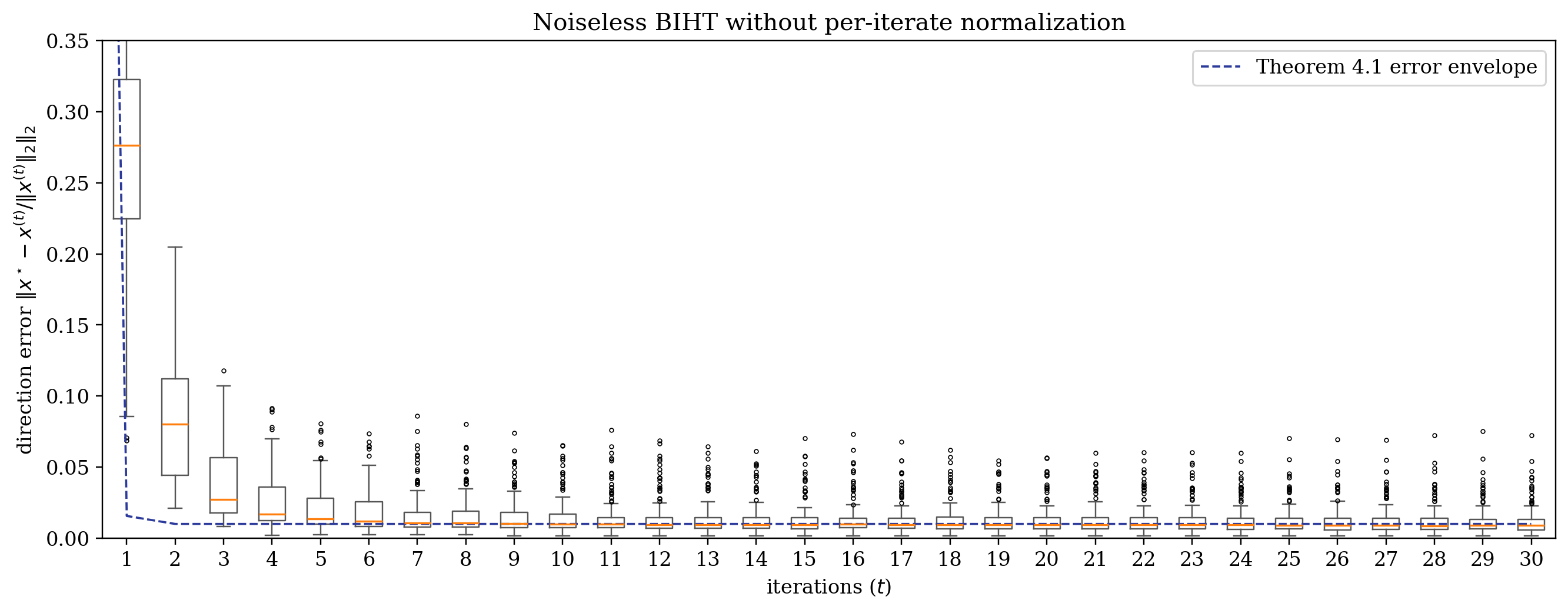

Figure 1: Numerical experiments illustrating the two regimes studied in the paper: finite-time convergence without normalization in the noiseless case, and early recovery under sign corruptions.. a — Noiseless measurements. Boxplots show the directional error of BIHT[1] for \(t=1,\ldots,30\) over \(100\) independent trials.The dashed curve is the error envelope from 4, with \(\epsilon = 0.01\)., b — A uniformly random \(\tau=0.1\) fraction of measurements is flipped, and we compare unnormalized BIHT with the per-iterate normalized variant. Boxplots show the directional error over \(100\) independent trials with \(n=2000\), \(s=5\), \(m=1000\), and \(60\) iterations. The dashed curve is the constants-suppressed rate guide from 6, and the dotted vertical line marks the corresponding stopping time.