Robust Peak-cost Constrained Reinforcement Learning
July 16, 2026
Abstract
We study robust peak-cost constrained reinforcement learning (RP-CRL), where the objective is to maximize expected reward while controlling the maximum cost encountered along a trajectory. This setting is motivated by safety-critical applications in which a single large violation can be catastrophic and therefore cannot be adequately captured by the standard CMDP framework based on expected cumulative cost. Existing reachability-constrained RL methods adopt Lagrangian-based approaches, yet the underlying duality properties of peak-cost constrained MDPs remain unclear. We show that, unlike standard CMDPs, peak-cost constrained MDPs may not admit zero duality gap. We further consider a robust formulation to address simulator-to-real-world mismatch in the transition dynamics. To solve this problem, we develop a surrogate optimization framework and a robust value estimation method based on integral probability metrics. We prove that, with appropriate hyperparameter choices, the surrogate solution attains the same robust reward value as the original problem while violating the constraint by at most \(\epsilon\). Experiments show that the proposed method effectively enforces safety under dynamics perturbations while retaining strong reward performance.
1 Introduction↩︎
Safety is a fundamental requirement in intelligent decision-making problems. Motivated by this, recent reinforcement learning (RL) research has extensively studied constrained Markov decision processes (CMDPs) [1]–[4]. In the standard CMDP framework, safety is enforced by requiring the expected cumulative cost to remain below a prescribed threshold. However, this formulation is insufficient for many practical applications, where the primary concern is not the total accumulated cost, but rather the largest cost incurred along a trajectory. In such settings, even a single large violation can be catastrophic, regardless of how small the cumulative cost is overall. For example, a trajectory may incur small costs at most time steps but experience one severe safety violation, making it significantly more dangerous than another trajectory whose maximum cost remains uniformly bounded.
To address this limitation, recent works [5], [6] have considered reachability-constrained reinforcement learning (RCRL), where the goal is to maximize expected reward subject to a peak-cost constraint, namely that the maximum cost encountered along a trajectory remains below a specified threshold (often \(0\)). These works develop Lagrangian-based methods for solving the resulting optimization problem. However, unlike the standard CMDP setting, where zero duality gap is well established, such a guarantee has not been shown for peak-cost constrained MDPs. As a result, it remains unclear whether these Lagrangian-based approaches can recover the true optimal solution.
An additional limitation of existing work is that it does not account for uncertainty in the transition dynamics [5], [6]. In practice, policies are often trained in simulation and then deployed in the real world, where the true dynamics may differ from those of the simulator. Consequently, a policy that satisfies the peak-cost constraint in simulation may still violate the same constraint after deployment due to model mismatch. This motivates the following central questions:
Does a peak-cost constrained MDP admit zero duality gap? How can we develop an algorithm for the robust peak-cost constrained problem that bridges the sim-to-real gap?
Our Contributions:
We show that, unlike the standard CMDP, a peak-cost constrained MDP may fail to admit zero duality gap, even in a two-state MDP. The key reason is that convexity with respect to the state-action occupancy measure breaks down.
We formulate a robust peak-cost constrained problem and propose a surrogate optimization framework. We show that, with appropriate hyperparameter choices, the optimal solution of the surrogate problem achieves the same robust reward value as the original problem while violating the constraint by at most an \(\epsilon\)-amount.
We develop an effective approach for estimating the robust value function based on an integral probability metric. Empirically, we show that the proposed method can effectively satisfy the constraint even when the environment is perturbed.
1.1 Related Works↩︎
CMDP : Constrained Markov Decision Processes (CMDPs) are a foundational framework for solving constrained reinforcement learning (CRL) problems [1]. CMDPs leverage the convexity of the state-action occupancy measure, enabling the use of primal-dual methods to solve the optimization problem [4], [7]–[9]. These methods have well-established convergence guarantees and have been extensively studied in the literature [2], [3], [10]. Beyond primal-dual methods, linear programming (LP)-based and model-based approaches have also been explored, directly addressing the primal problem [11]–[13]. However, peak-constained objective is different compared to the CMDP.
RCMDP: Unlike standard CMDPs, the optimization problem for RCMDPs is non-convex in the state-action occupancy measure, which complicates the use of traditional Lagrangian or primal-dual methods [14]. Some studies have attempted to address this challenge using primal-dual methods under strong duality assumptions, but these approaches often lack iteration complexity guarantees [15]. Recent work has introduced epigraph reformulations to address the limitations of primal-dual methods, but these approaches require computationally expensive binary search procedures and are sensitive to noise in policy value estimation [16]. [17] avoids these limitations by jointly optimizing for robustness and constraint satisfaction, eliminating the need for binary search with iteration guarantees. However, these methods do not consider peak cost constraint which we consider.
Feasible Sets and Reachability Analysis for Safety and Optimality in CMDPs: Characterizing feasible sets is a critical and ongoing challenge in safe control and reinforcement learning [18]. Feasible sets, often represented using safety certificates like control barrier functions (CBFs) [19], [19], [20], define the set of states from which the system can recover to safety. However, energy-based safety certificates often result in overly conservative or inaccurate feasible sets, limiting their applicability [21]. Hamilton Jacobian (HJ) reachability analysis provides a more rigorous approach to deriving feasible sets but is computationally expensive due to the non-trivial partial differential equations involved [22]. Recently, RL-based approaches are considered to find policy that will avoid unsafe sets [23]–[25], however, they did not consider on maximizing reward as an objective. [5], [6] learns a single policy that balances safety and optimality,considering peak cost constraint optimization. They used Lagrangian framework to solve the problem, however, they did not provide any strong duality guarantee. Further, none of the above work considered robust optimization framework bridging the sim-to-real gap while being trained on the simulator model which might be different from the real environment.
2 Preliminaries and Problem Formulation↩︎
2.1 Constrained Markov Decision Processes↩︎
A Constrained Markov Decision Process (CMDP) is defined by \[M=\langle \mathcal{S},\mathcal{A},P,r,c,\gamma,d_0\rangle,\] where \(\mathcal{S}\) and \(\mathcal{A}\) denote the state and action spaces, \(P(\cdot\mid s,a)\) is the (possibly unknown) transition kernel, \(r:\mathcal{S}\times\mathcal{A}\to\mathbb{R}\) is the reward function, \(c:\mathcal{S}\times\mathcal{A}\to\mathbb{R}\) is the cost function, \(\gamma\in(0,1)\) is the discount factor, and \(d_0\) is the initial state distribution. A policy is denoted by \(\pi(\cdot\mid s):\mathcal{S}\rightarrow \Delta(\mathcal{A})\).
For a given transition model \(P\) and policy \(\pi\), let \(V_r^{P,\pi}(s)\) and \(V_c^{P,\pi}(s)\) denote the discounted negative reward and cost value functions, respectively: \[V_r^{P,\pi}(s) = -\mathbb{E}\!\left[ \sum_{t=0}^{\infty}\gamma^t r(s_t,a_t)\,\middle|\, s_0=s,\pi,P\right],\] \[V_c^{P,\pi}(s) = \mathbb{E}\!\left[\sum_{t=0}^{\infty}\gamma^t c(s_t,a_t)\,\middle|\, s_0=s,\pi,P\right].\] The corresponding objective values from the initial distribution \(d_0\) are \[J^P_r(\pi)=\mathbb{E}_{s\sim d_0}\!\left[V_r^{P,\pi}(s)\right], \quad J^P_c(\pi)=\mathbb{E}_{s\sim d_0}\!\left[V_c^{P,\pi}(s)\right].\]
A standard CMDP seeks to maximize reward while keeping the expected discounted cost below a budget \(b\). Corresponding to discounted negative reward, the CMDP objective becomes: \[\min_{\pi}\; J^P_r(\pi) \qquad \text{s.t.}\qquad J^P_c(\pi)\le b.\] When Slater’s condition holds, the standard CMDP admits zero duality gap [26], and therefore Lagrangian-based methods provide an effective solution approach.
2.2 Peak-Cost Constraints↩︎
Although CMDPs are widely used, a major limitation is that the constraint is expressed only through the expected cumulative discounted cost. In many applications, however, controlling only the cumulative cost is insufficient; instead, one must ensure that the maximum cost encountered along a trajectory remains below a desired threshold.
Concrete example (reachability and persistent safety) In many safety-critical settings, we require that the system never enter an unsafe region. Let \(c(s)\) be a state-based safety function such that \(c(s)\le b\) for safe states and \(c(s)>b\) for unsafe states. Then, for a policy \(\pi\), safety along a trajectory \(\tau=(s_0,s_1,\dots)\sim\pi\) requires \(\max_{t\in\mathbb{N}} c^{\pi}(s_t)\le 0\) with probability \(1\) where \(b\) is some safety threshold. That is, the maximum safety violation encountered along the trajectory must remain non-positive.
Motivated by this, we consider the following peak-constrained problem: \[\min_{\pi}\; J_r^P(\pi) \qquad \text{s.t.}\qquad \max_{s\in \mathcal{S}^{\pi,P}} c(s)\le b,\] where \(\mathcal{S}^{\pi,P}=\{s\in \mathcal{S}:\Pr(\exists t\geq 0, s_t=s|s_0\sim d_0,\pi,P)>0\}\). We assume that the initial states always give you at least one policy which is feasible. Often times, we consider an episodic setup with length \(T\) then \(t\) will be upper bounded by \(T\).
Note that the peak constraint is difficult to evaluate as one needs to predict the future states at a given time \(t\). Reference [23] first observed that, for a fixed policy \(\pi\), this peak-cost constraint can be represented through a value function using a discounted recursion. In particular, define \[\begin{align} Q_{c,\mathrm{peak}}^{\pi,P}(s,a) &= (1-\gamma)c(s) \notag \\ & + \gamma \max\left\{c(s),\,\mathbb{E}_{P(\cdot\mid s,a)}\left[V_{c,\mathrm{peak}}^{\pi,P}(\cdot)\right]\right\} \label{eq:max95value} \end{align}\tag{1}\] and \[V_{c,\mathrm{peak}}^{\pi,P}(s)=\langle \pi(\cdot\mid s),Q_{c,\mathrm{peak}}^{\pi,P}(s,\cdot)\rangle. \label{eq:q95value}\tag{2}\] For \(\gamma<1\), the operator induced by 1 is a contraction, and hence \(V_{c,\mathrm{peak}}^\pi\) can be computed for a given policy \(\pi\) by fixed-point iteration. For finite-horizon episodic setup, we can simply take \(\gamma=1\).
This leads to the following modified optimization problem: \[\begin{align} \label{eq:rcrl} \min_{\pi}\; J^P_r(\pi) \qquad \text{s.t.}\qquad \max_{s\in \mathcal{S}^{\pi,P}}\!\left[V_{c,\mathrm{peak}}^{\pi,P}(s)\right]\le b. \end{align}\tag{3}\] A related formulation was also considered by [5]. They proposed the following Lagrangian-based objective: \[\begin{align} \min_{\pi}\max_{\beta\ge 0}\; \!\left[V_r^{\pi,P}(s)+\beta(s)V_{c,\mathrm{peak}}^{\pi,P}(s)\right], \label{eq:lagrangian} \end{align}\tag{4}\] where \(\beta(s)\) is a state-dependent Lagrange multiplier used to penalize constraint violations.
2.3 Limitations of the Lagrangian Approach in [5]↩︎
While [5] adopts the Lagrangian formulation in 4 , it does not establish a strong-duality guarantee. This is a critical issue because the peak-cost constrained problem is fundamentally different from the standard CMDP: the constraint is no longer based on an additive discounted cumulative cost, but instead depends on the maximum cost encountered along a trajectory. In particular, the reachability set \(\mathcal{S}^{\pi,P}\) inherently depends on the policy \(\pi\).
In this paper, we show that the peak-cost constrained problem does not necessarily admit zero duality gap. To the best of our knowledge, this is the first result showing that, unlike the standard CMDP, the peak-constrained problem may fail to satisfy strong duality. The key reason is that the problem is no longer convex in the state-action occupancy measure, due to its dependence on the trajectory-wise maximum cost.
Theorem 1. [informal] The problem stated in (3 ) may have a non-zero duality gap even if the Slater’s condition is satisfied.
The proof of Theorem 1 is in Appendix 6.1.
Remark 1 (Implication for primal-dual methods). Theorem 1 shows that the modified hard-max constraint can destroy the strong-duality structure that underlies standard primal-dual methods for CMDPs. In ordinary CMDPs, the objective and constraints are linear in the discounted state-action occupancy measure, which yields a convex primal problem and zero duality gap under mild conditions. By contrast, the modified hard-max constraint induces a nonlinear, nonstandard feasible set, and the associated Lagrangian relaxation can be strictly loose. Consequently, a primal-dual method applied directly to this modified constraint is not, in general, guaranteed to recover the true constrained optimum. This observation motivates the use of alternative surrogate formulations and direct policy-space optimization methods for such peak-style safety objectives.
2.4 Limitations and a Robust Formulation↩︎
Problem (3 ) does not account for the mismatch between the simulated environment used for training and the real environment in which the learned policy is ultimately deployed. In practice, policies are often trained in simulation and then transferred to the real world, where the transition dynamics may differ from those of the simulator. As a result, a policy that appears feasible in simulation may violate the safety constraints after deployment. This motivates a robust formulation in which the learned policy must remain feasible under the worst-case model within a prescribed uncertainty set. Accordingly, we consider the following robust counterpart: \[\begin{align} \label{eq:robust95rcrl} \min_{\pi}\max_{P\in \mathcal{P}}\; J_r^{P}(\pi) \qquad \text{s.t. } \max_{P\in \mathcal{P}}\max_{s\in \mathcal{S}^{\pi,P}}\!\left[V_{c,\mathrm{peak}}^{\pi,P}(s)\right]\le b. \end{align}\tag{5}\] This formulation seeks to maximize the worst-case expected cumulative reward while ensuring that the worst-case peak constraint remains below the prescribed threshold.
For the uncertainty set, one natural choice is the rectangular uncertainty set \[\mathcal{P}_{(s,a)} = \left\{ P \in \Delta(S) : D\!\left(P, P_0(\cdot \mid s,a)\right) \leq \rho \right\},\] where \(D(\cdot,\cdot)\) measures the distance between two probability distributions, and \(P_0\) is the nominal model encountered in simulator. Rectangular uncertainty sets are particularly attractive because they often lead to tractable robust dynamic programming formulations, whereas evaluating the robust value function under non-rectangular uncertainty sets is, in general, NP-hard [27].
For continuous state spaces, one may instead consider uncertainty sets defined through an integral probability metric (IPM) [28], which admits an efficient representation of the worst-case value function under linear function approximation. In particular, the IPM between two distributions \(p\) and \(q\) is defined as \[d_F(p,q) = \sup_{f\in F}\left\{p^\top f - q^\top f\right\}, \qquad F \subseteq \mathbb{R}^{|S|}.\] Under suitable choices of \(F\), the IPM recovers important distributional distances; for example, under special conditions it reduces to the total variation distance [29]. Moreover, IPM-based uncertainty sets yield a closed-form expression for the robust Bellman operator under linear approximation for value function (i.e., \(V_{c,\mathrm{peak}}^{\pi}(s)=\Psi(s)^Tw^{\pi,c}\)) \[L_P V_{c,\mathrm{peak},w}^{\pi} = (1-\gamma)c(s,a) + \gamma V_{c,\mathrm{peak},w}^{\pi} + \rho \|w_{c,2:d}\|_2. \label{eq:IPM}\tag{6}\] Here, \(L_P\) is the worst case robust Bellman operator, defined as \(L_p V_{c,\mathrm{peak}}^\pi = c(s,a)+ \sup_{P}\langle P (\cdot|s,a),V_{c,\mathrm{peak}}^{\pi,P}(\cdot)\rangle\)
3 Solution Methodology↩︎
In this section, we discuss our problem to solve peak-cost constrained robust MDP as described in (5 ).
3.1 Robust Peak-Cost Constrained MDP Formulation↩︎
Note that since the problem in (3 ) may not have a zero duality gap we have to consider a surrogate problem. Inspired from [17], we consider the following surrogate problem for \(\beta>0\). \[\min_{\pi} \max\{\max_{P} J_r^{\pi,P}/\beta, (\max_{P,s\in \mathcal{S}^{\pi,P}} V_{c,\mathrm{peak}}^{\pi,P}(s)-b)\}\label{eq:main95obj}\tag{7}\] [17] adopted this surrogate problem for the robust CMDP problem, here, we apply for the robust peak cost constrained problem. Note that when the policy \(\pi\) is infeasible and \(\beta\) is large enough, then, it would try to optimize the constraint value function to make it satisfy the constraint. On the other hand, when the policy is feasible then it would optimize the objective if the reward is positive if the peak-cost constraint is satisfied.
The effectiveness of the surrogate problem in (7 ) is shown in the following proposition.
Proposition 1. Let \(\hat{\pi}^*\) be an optimal solution of (7 ), then \(J_r^{\hat{\pi^*}}\geq J_r^{\pi^*}\) where \(\pi^*\) is an optimal solution for (5 ). Further if \(\beta\geq C_\text{max}/\epsilon\), then \((\max_{P,s\in \mathcal{S}^{\pi,P}}V_{c,\mathrm{peak}}^{\pi,P}(s)-b)_+\leq \epsilon\).
The above proof is adapted from Proposition 1 in [17], and has been shown in Appendix 6.1. [17] also provides the convergence rate guarantee for a robust natural policy gradient which solves (7 ) for the finite state-space. Our goal is to apply for the large state-space problem, hence, we do not consider the natural policy gradient. We rather consider an robust actor-critic-based approach, and we use PPO-method [30] for the actor.
4 Proposed Algorithm↩︎
In this section, we present our approach for solving the robust peak-constrained MDP problem formulated in 7 . Our algorithm is based on the Actor-Critic framework modified for the peak-constrained, and the robust value function.
4.1 Actor–Critic Optimization↩︎
To account for robustness, we adapt the temporal-difference (TD) errors for both the reward critic and the peak-cost critic using the IPM-based robustification in 6 . Specifically, we copnsider the following advantage function \[\begin{align} \delta_{t,r} &= r_t + \gamma V_r(s_{t+1}) - V_r(s_t) + \rho_r \|w_{r,2:d}\|_2, \tag{8} \\ \delta_{t,c} &= \big(1-\gamma \big)c_t+ \gamma \max\!\big(c_t,\, V_{c,\mathrm{peak}}(s_{t+1})\big) \nonumber \\ & \qquad \qquad \qquad - V_{c,\mathrm{peak}}(s_t) + \rho_c \|w_{c,2:d}\|_2. \tag{9} \end{align}\] Note that the added regularization is due to the robust value function metric as discussed in (6 ). For smooth approximation, instead of max operator, we use Log-Sum-Exponential(LSE).
Using these TD errors, we construct the generalized advantage estimates (GAEs) for the reward objective and 1-step advantage estimate for peak-cost objective as \[\begin{align} A_{t,r} &= \sum_{l=0}^{\infty} (\gamma \lambda)^l \delta_{t+l,r}, \tag{10} \\ A_{t,c} &= \delta_{t,c}. \tag{11} \end{align}\]
Here \(\lambda\) is the GAE decay. The corresponding value targets for the reward and peak-cost critics are given by \[\begin{align} v_{\text{target},r}(s_t) &= A_{t,r} + V_r(s_t), \tag{12} \\ v_{\text{target},c}(s_t) &= A_{t,c} + V_{c,\mathrm{peak}}(s_t) \tag{13} \end{align}\]
The actor is updated using the PPO-style clipped objective [30] depending on whether we are optimizing the objective or the constraint \[\begin{align} L_{\text{actor}} = \mathbb{E}_t \!\left[ \min\!\left( r_t(\theta)\, A_{t,j},\; \mathrm{clip}\!\big(r_t(\theta),\, 1-\epsilon,\, 1+\epsilon\big)\, A_{t,j} \right) \right], \label{eq:actor95loss} \end{align}\tag{14}\] where \(r_t(\theta)\) denotes the policy ratio and \(A_{t,j}\) is the advantage signal used for the policy update, for \(j=r,c\).
The robust critic losses for the reward and peak-cost value functions are defined as \[\begin{align} L_{V_r} &= \Big(V_r(s_t) - v_{\text{target},r}(s_t)\Big)^2, \tag{15} \\ L_{V_{c,\mathrm{peak}}} &= \Big(V_{c,\mathrm{peak}}(s_t) - v_{\text{target},c}(s_t)\Big)^2. \tag{16} \end{align}\]
Algorithm 1 summarizes the complete training procedure for the robust peak-constrained MDP.
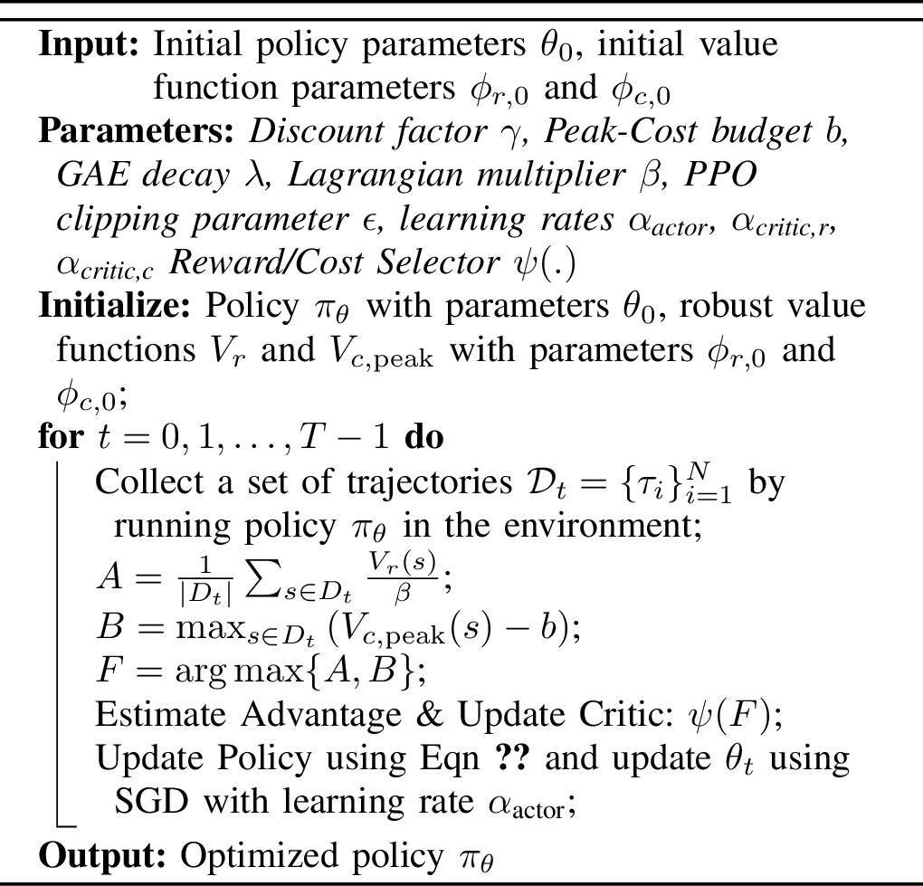
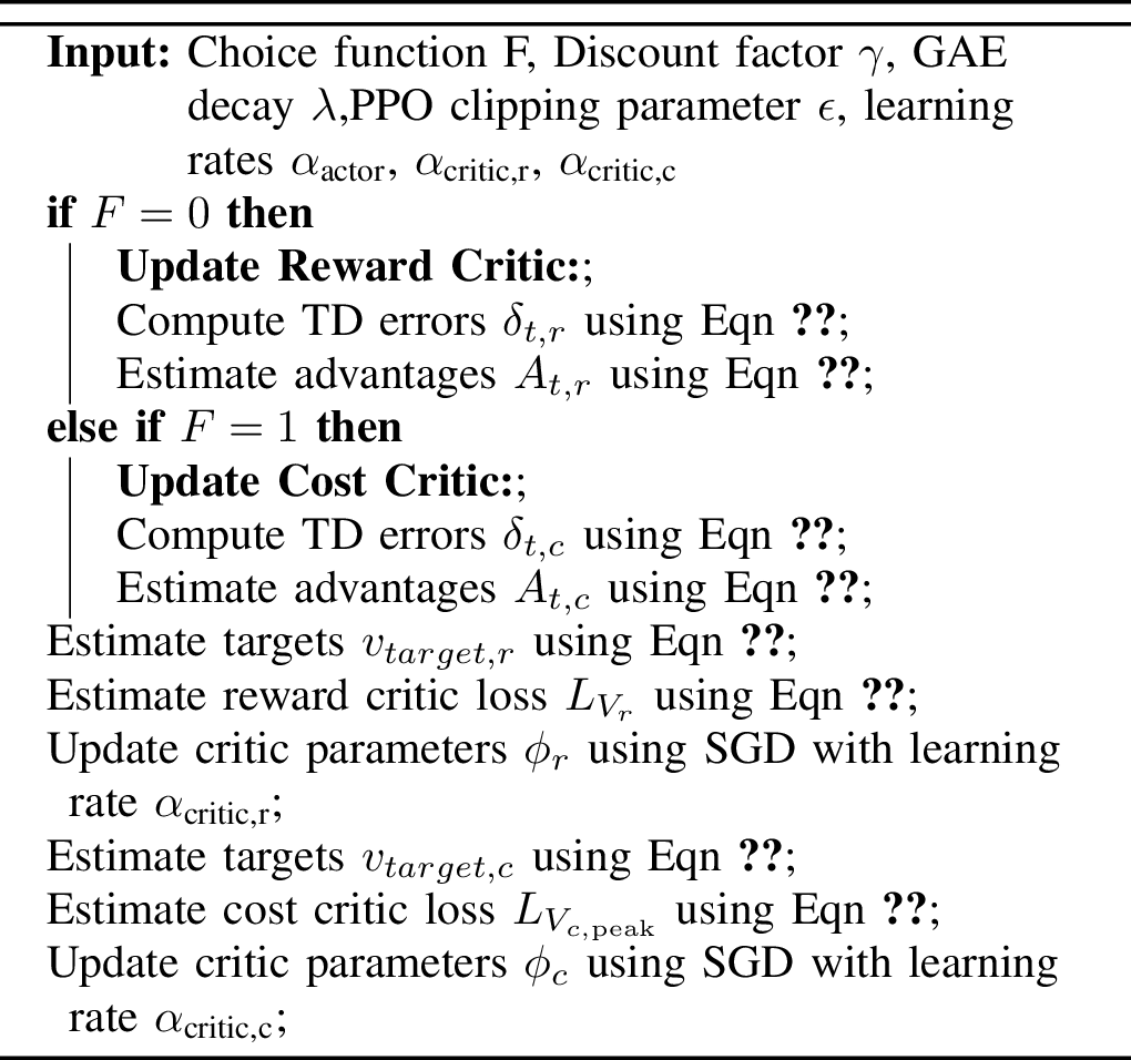
. Note that we take a sample average of the reward value function scaled by \(1/\beta\) (\(A\)), if it is higher than the maximum value function corresponding to the state sampled from the trajectory, then we update the actor based on the average reward value function, otherwise we update the actor based on the constraint value function to minimize the constraint violation.
5 Experiments↩︎
5.1 Baselines↩︎
We compare RP-CRLwith two baselines:
Primal Dual method for Peak-Cost Constraint which is used in [5], [6].
Using Surrogate Objective in 7 trained in Non-Perturbed environment
RP-CRLrefers to Surrogate Objective trained on Perturbed Environment.
5.2 OpenAI Gym Environment Results↩︎
The CartPole environment is a widely used reinforcement learning (RL) benchmark introduced in OpenAI Gym [31]. It consists of a cart
moving along a frictionless track, with a pole attached to the cart by an unactuated joint. The agent applies forces to the cart to move it left or right, aiming to balance the pole upright while keeping the cart within specified boundaries.
Constrained CartPole Environment In our work, we use a modified version of the standard CartPole environment by introducing safety and cost constraints. The state space remains the same as the standard CartPole and is
represented as: \(\text{Observation\;Space} = \{ (x, \dot{x}, \theta, \dot{\theta}) \mid x, \dot{x}, \theta, \dot{\theta} \in \mathbb{R} \}.\) where \(x\) is the cart position, \(\dot{x}\) is the cart velocity, \(\theta\) is the pole angle in radians, and \(\dot{\theta}\) is the pole angular velocity. The observation space is continuous
and unbounded. The action space differs from the standard environment. Instead of discrete actions (\(\{0, 1\}\)), we use a continuous action space where the agent can apply a force \(F \in [-10.0, 10.0]\).
The dynamics of the CartPole system are given by the following equations. The angular acceleration of the pole is: \[\ddot{\theta} = \tfrac{g \sin \theta + \cos \theta \left( -F - m_p l \dot{\theta}^2 \sin \theta \right) / (m_c + m_p)}{l \left( \tfrac{4}{3} - \tfrac{m_p \cos^2 \theta}{m_c + m_p} \right)},\] and the horizontal acceleration of the cart is: \[\ddot{x} = \tfrac{F + m_p l \left( \dot{\theta}^2 \sin \theta - \ddot{\theta} \cos \theta \right)}{m_c + m_p}.\] For our experiments, \(g = 9.8 \, \text{m/s}^2\) is the gravitational acceleration, \(m_c = 1.0 \, \text{kg}\) is the cart’s mass, \(m_p = 0.1 \, \text{kg}\) is the pole’s mass, and \(l = 0.5 \, \text{m}\) is the half-length of the pole. The time step for simulation is \(\tau = 0.02 \, \text{s}\).
The constrained environment enforces safety by requiring the cart’s position to remain within safe zone \(x \in [-1, 1]\). In general the pole angle should stay within \(x \in
[-2.4,2.4]\) and \(\theta \in [-12^\circ, 12^\circ]\). If these limits are exceeded before 450 steps, the episode terminates early, and an early termination penalty of \(10.0\) is added to the total cost. The agent incurs a cost when the cart’s position exceeds \(|x| > 1.0\), with the cost proportional to the absolute distance from the center: \[\text{cost} =
\begin{cases}
|x| & \text{if } |x| > 1.0 \\
10 & \text{if early termination}
\end{cases}\] The objective is to maximize cumulative rewards while keeping the peak cost below a predefined baseline. The maximum episode length is 500 steps.
Perturbed CartPole Environment To model transition uncertainty, we perturb gravity during training as \(g' = g + \mathcal{N}(0,0.5)\), requiring the policy to remain robust under uncertain
dynamics.
Training Details The architecture comprises three main networks: the Actor, the Critic, and the Peak-Cost Critic, each structured as a feedforward neural network with three layers (two hidden layers and one output layer). The Actor network features two hidden layers, each containing 64 neurons with a ReLU activation function, and it outputs parameters for the Gaussian distribution. Similarly, the Peak-Cost network consists of two hidden layers with 64 neurons each, utilizing a ReLU activation function, and it produces a single value representing the state value estimate. The Peak-Cost Critic follows the same architecture as the Critic, also featuring two hidden layers with 64 neurons and a ReLU activation function, outputting a single cost estimate. All the Actor and Critic networks use a learning rate of 3e-4.
5.3 Experiments and Analysis↩︎
For the experiments ([exp:pd95ours] and [exp:inference]), we used Lagrangian multiplier \(\beta= 25\), baseline \(b=2.0\), a warm start of 300 episodes(for RP-CRL).
Effectiveness of our Surrogate Objective
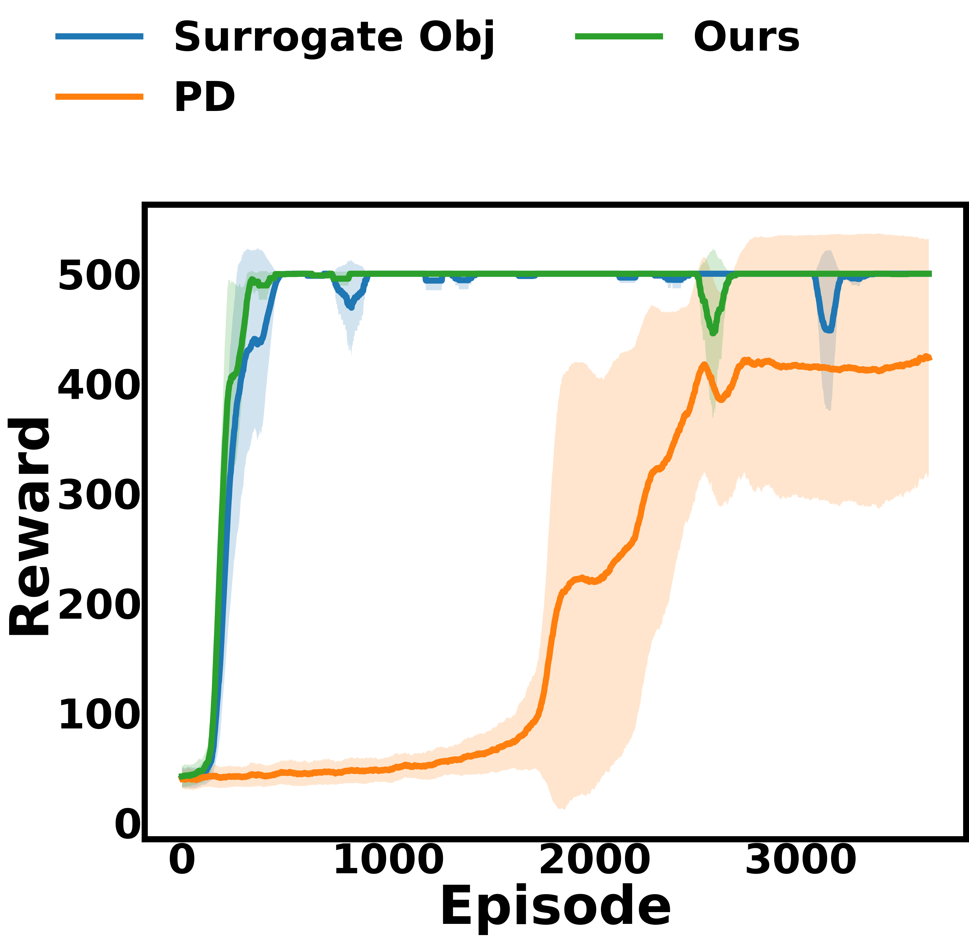
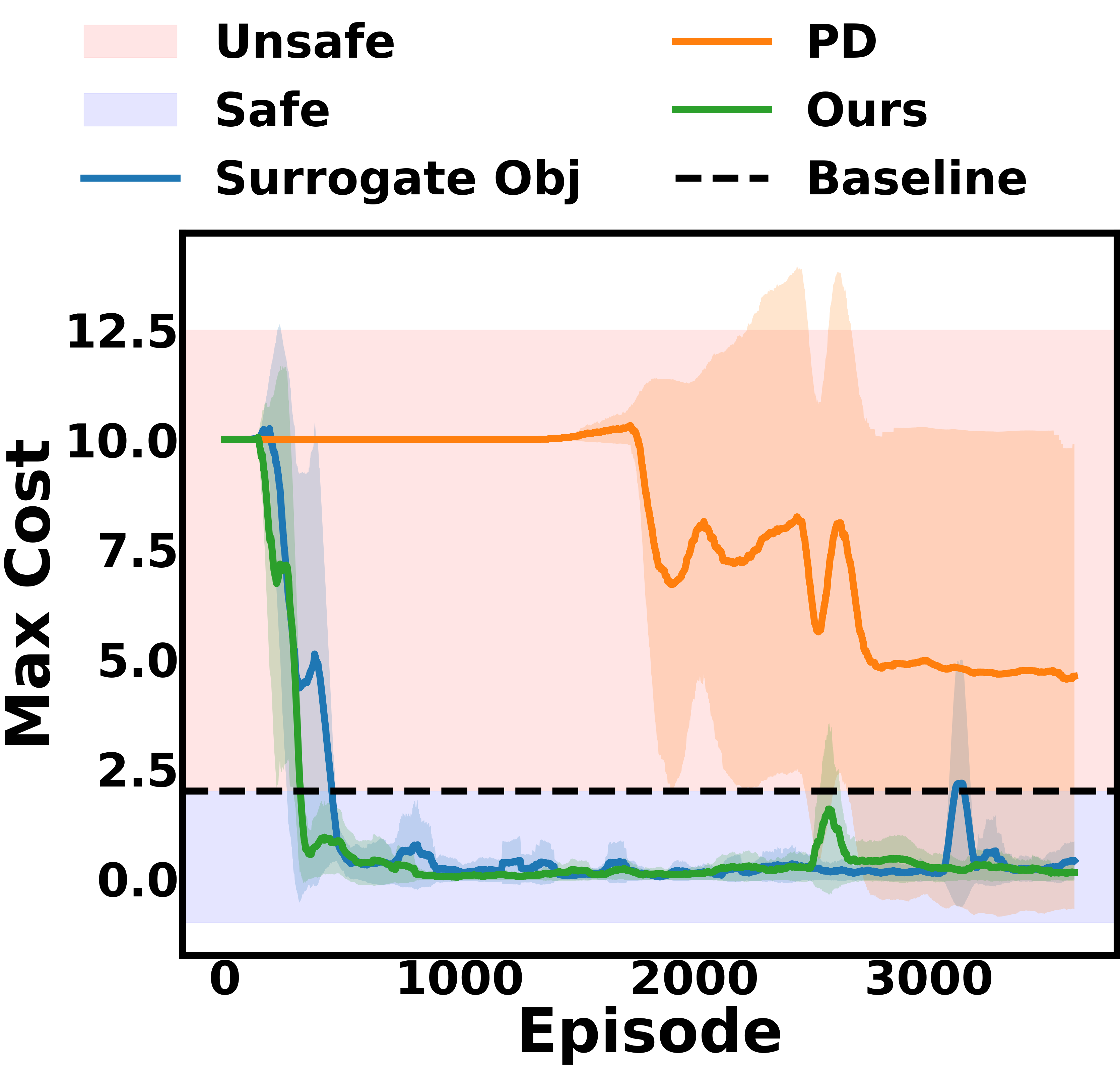
Figure 3: Comparison of Primal Dual(PD) and Surrogate Objective trained in non-perturbed environment, and RP-CRLtrained in perturbed CartPole environment. Here we want to maximize return while restrict peak-cost below baseline. RP-CRLhas learned peak-cost constraint and has higher rewards than PD.. a — Returns, b — Peak-Cost
Fig 3 compares the training of Primal-Dual (PD), Surrogate Objective in 7 on a non-perturbed CartPole environment and RP-CRL(Surrogate Objective trained on a perturbed CartPole environment). The Surrogate objective based methods successfully enforce the peak-cost constraint and achieve higher returns compared to PD. PD learns lower returns and has higher peak-cost than baseline because it learns a sub-optimal policy.
Inference in Perturbed Environment

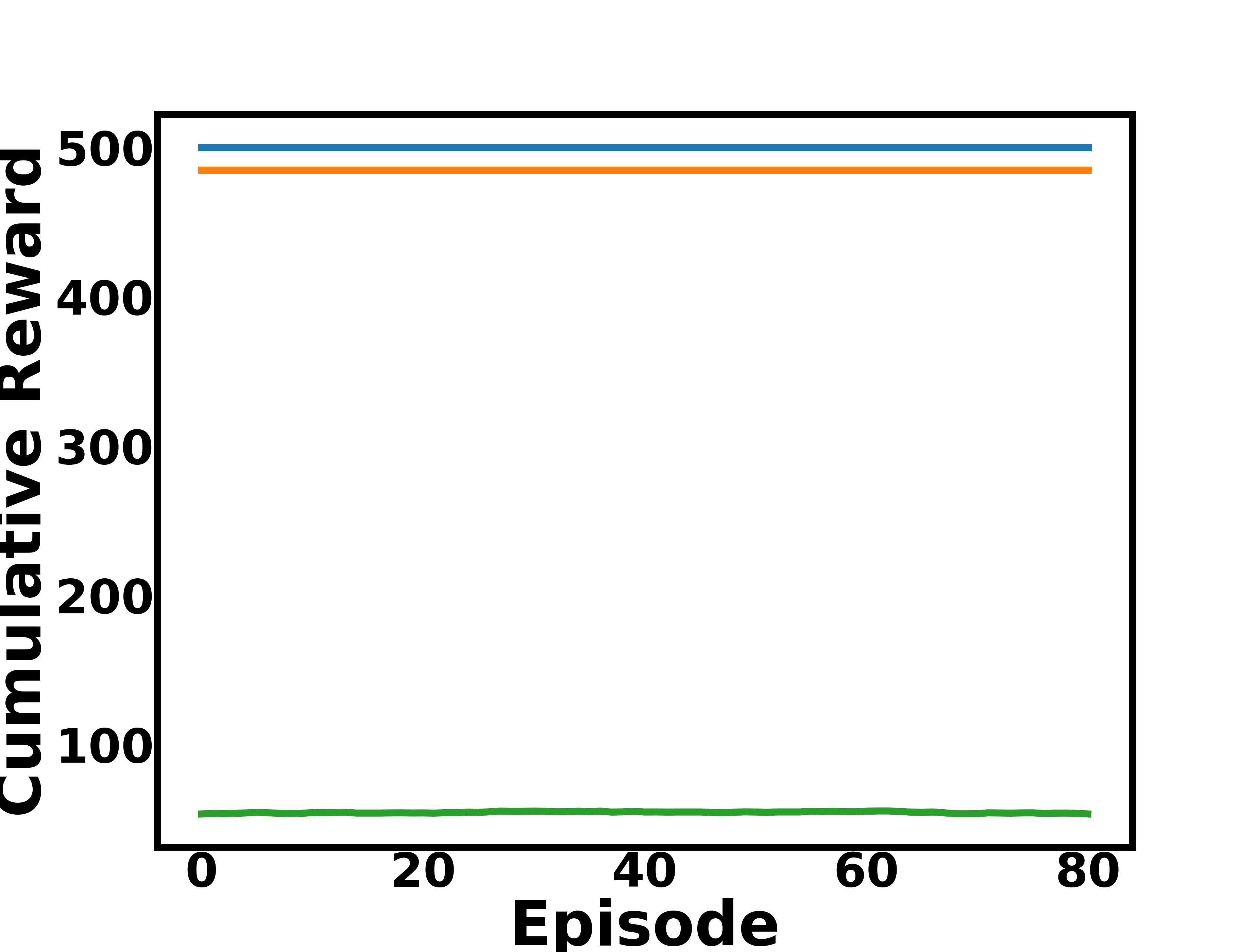
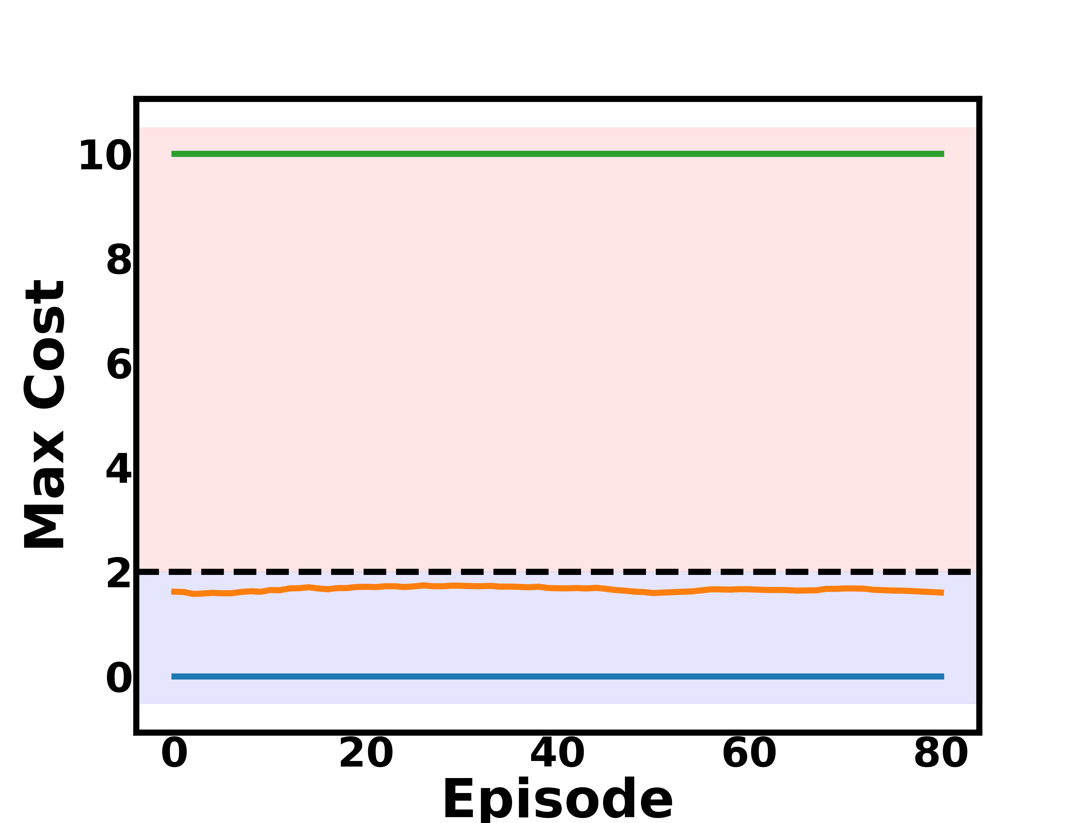
Figure 4: Comparison of inference performances of PD trained on non-perturbed(NP) environment, Surrogate Objective 7 trained on NP environment and RP-CRLtrained in perturbed (P) environment.RP-CRLperforms best with a peak-cost of zero. PD fails to adapt to a perturbed environment at inference.. b — Returns, c — Peak-Cost
The inference is done with a perturbation of \(g' = g + \mathcal{N}(0,2.0)\). The comparison in Fig 4 highlights the superior performance of RP-CRLtrained in a perturbed (P) environment, achieving the best results with a peak-cost of zero. In contrast, Surrogate Objective, trained in non-perturbed (NP) environments, has a peak-cost below baseline and PD fails to meet the peak-cost constraint and adapt to the robustness required during inference, evident from its rewards as well.
5.4 Training across Different Cost Functions↩︎
We perform a study of RP-CRLlearning two different cost functions to investigate the generalizability of training our proposed approach.
Cost1 (C1) : This cost penalizes deviations from the center and heavily penalizes early termination due to exceeding position or angle limits. A cost of equal to position error is incurred when the cart’s position exceeds a distance of 1 from origin. If the cart’s position is greater than 2.4 or pole angle is greater than \(12^\circ\) before the termination limit of 450 steps, a penalty of \(10.0\) is added to the cost. The baseline used for this cost is \(b=2\). Green line in Fig 3 shows training plots using C1 for RP-CRL.
Cost2 (C2) : This cost incentivizes staying within safe position and angle limits to avoid termination. It penalizes deviations in position greater than 1.0 from origin and pole angle greater than \(8^\circ\). These costs increase as they approach termination thresholds (position \(> 2.4\), angle \(> 12^\circ\)). The baseline used for this cost is \(b=0.5\). Fig 5 shows training plots using C2.
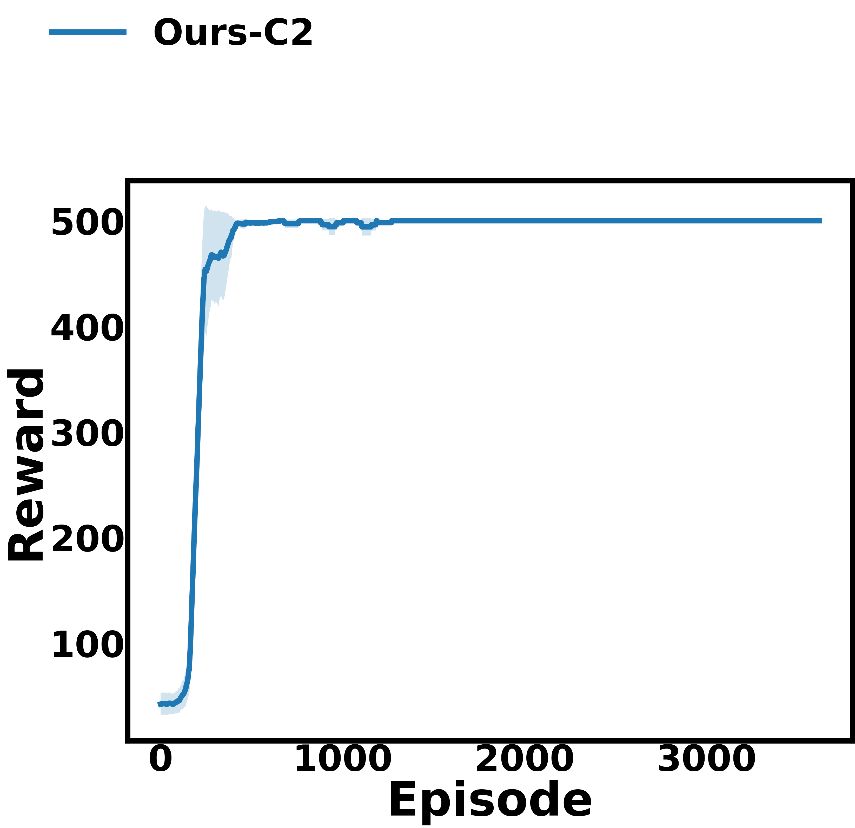
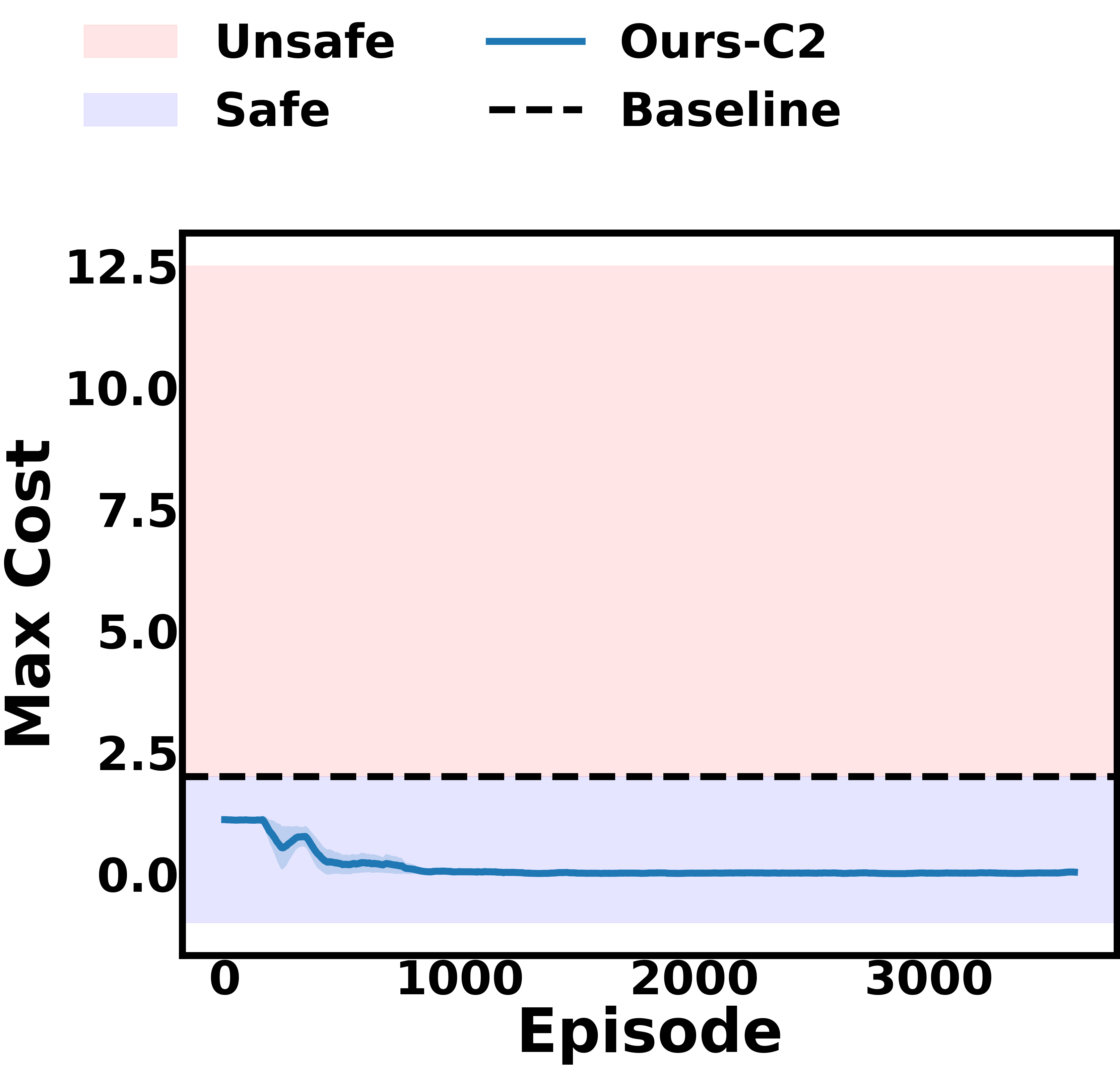
Figure 5: Learning RP-CRLon C2. The policy learns the peak-cost below baseline... a — Returns, b — Peak-Cost
These results demonstrate the robustness and adaptability of RP-CRLin effectively learning across different cost functions.
5.5 Training across Different Levels of Perturbations↩︎
We perform a study of RP-CRLlearning two different perturbation levels in the perturbed CartPole environment. This experiment is conducted to investigate how good RP-CRLlearns when perturbations in environment are different. Fig 6 shows the training curves for different perturbation levels. We perturb the gravity \(g' = g + \mathcal{N}(0,\sigma)\). For comparison, we consider \(\sigma = \{0.5,2\}\). The learning curves demonstrate RP-CRLlearns different perturbation levels effectively.
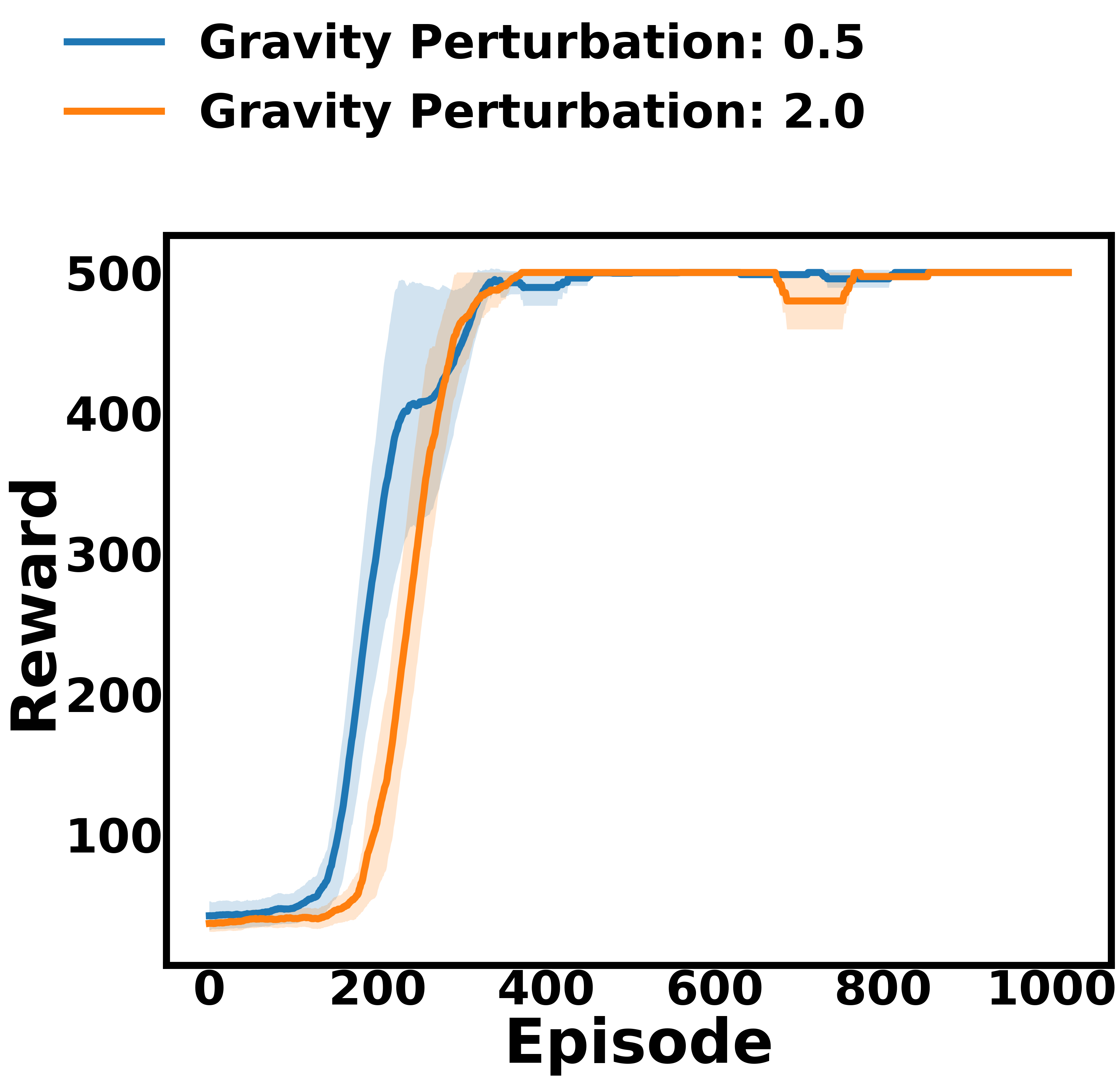
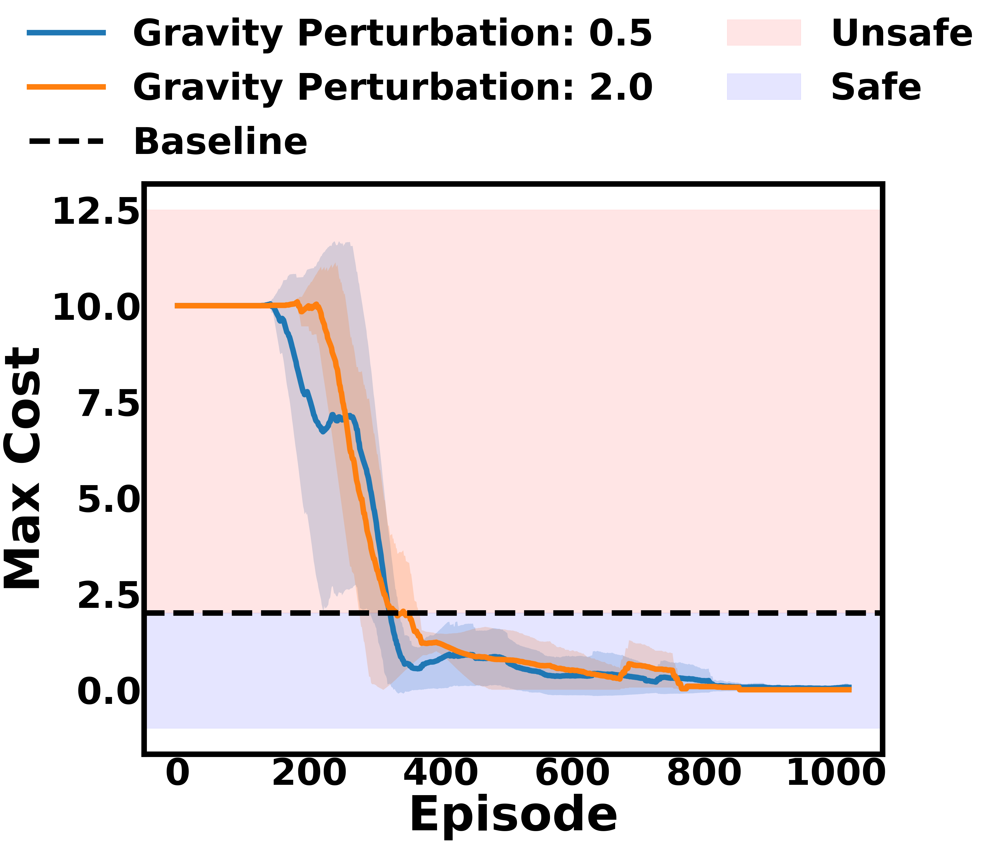
Figure 6: Comparison of training curves of RP-CRLfor different perturbation levels in the environment. The perturbation is introduced in gravity. RP-CRLlearns maximized returns and bounded peak-cost below baseline for both perturbation levels.. a — Returns, b — Peak-Cost
5.6 Mujoco Environment Results↩︎
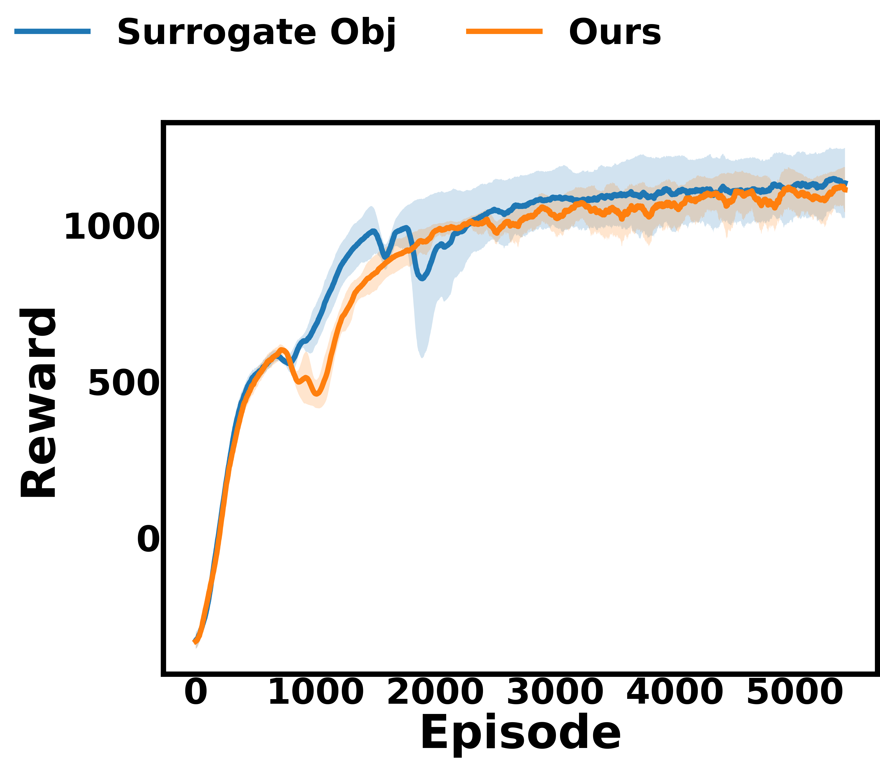
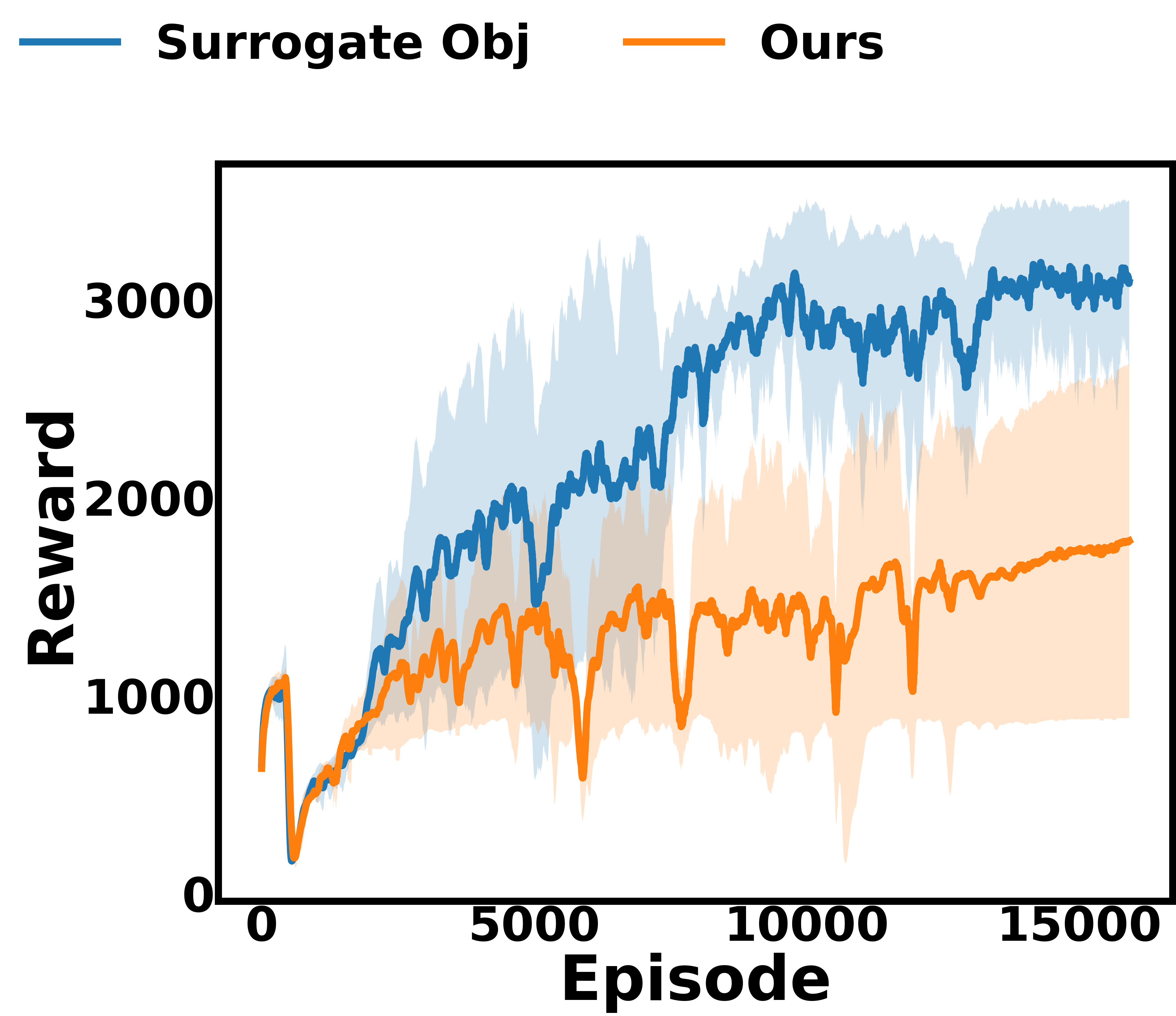
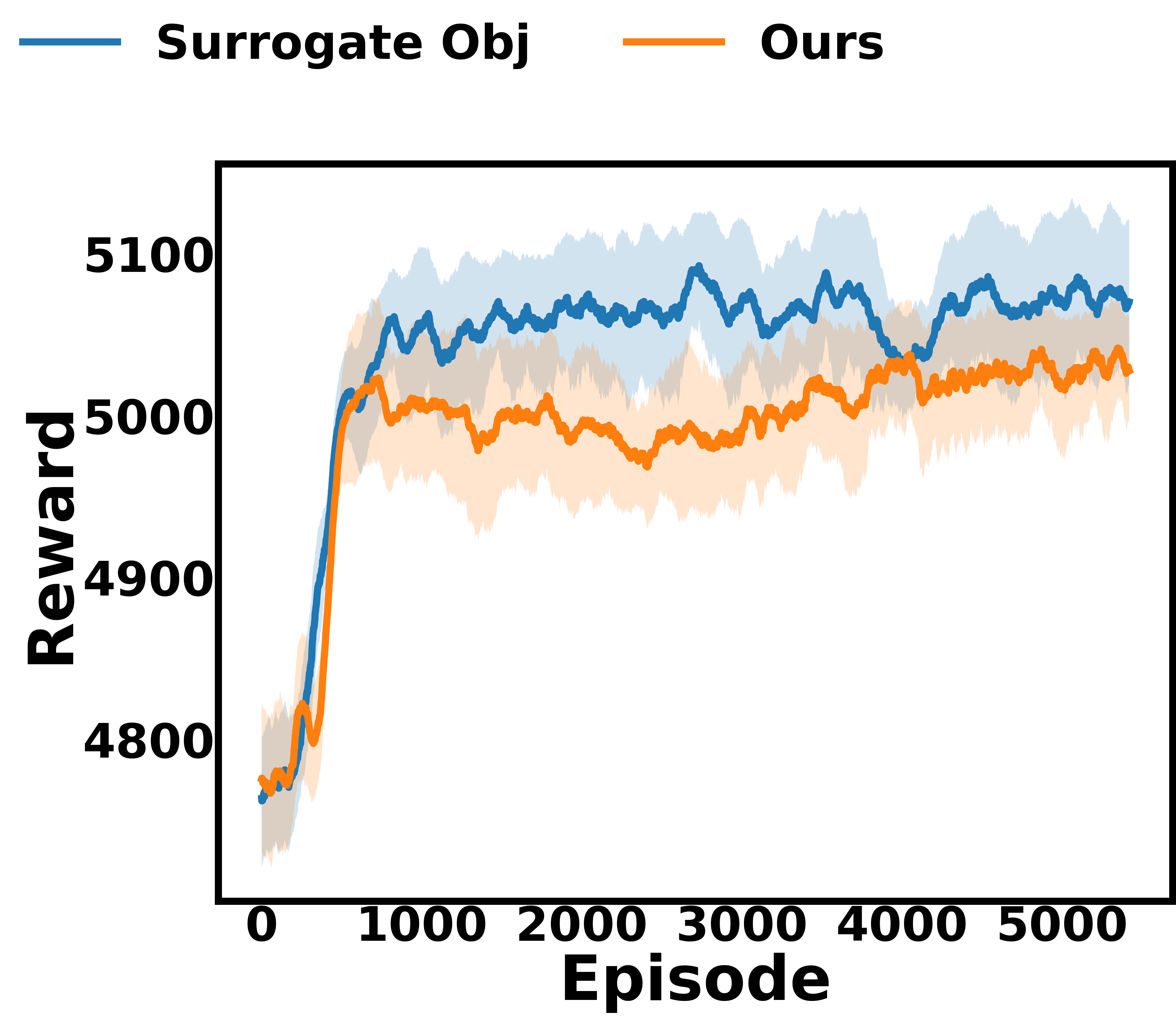
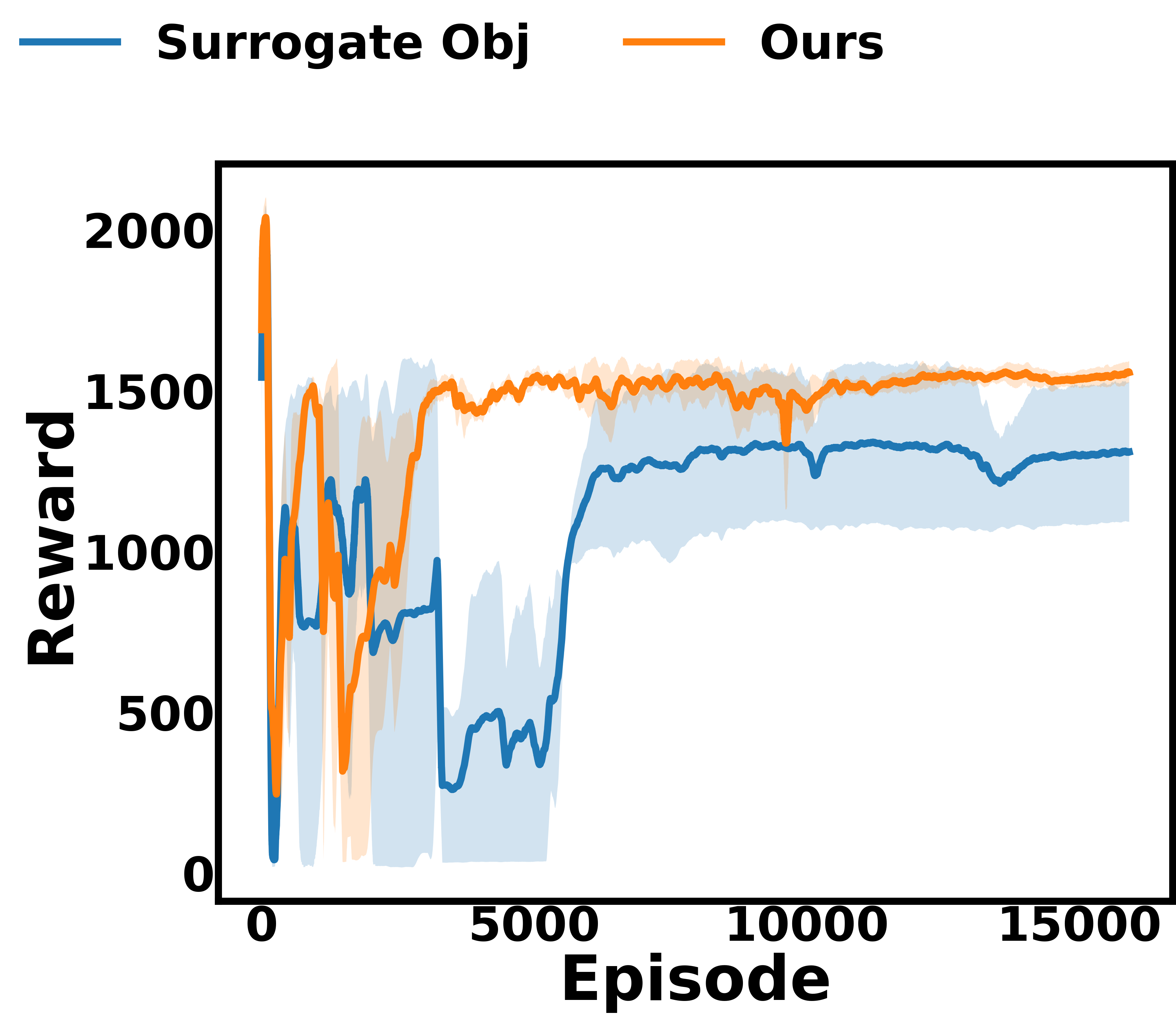

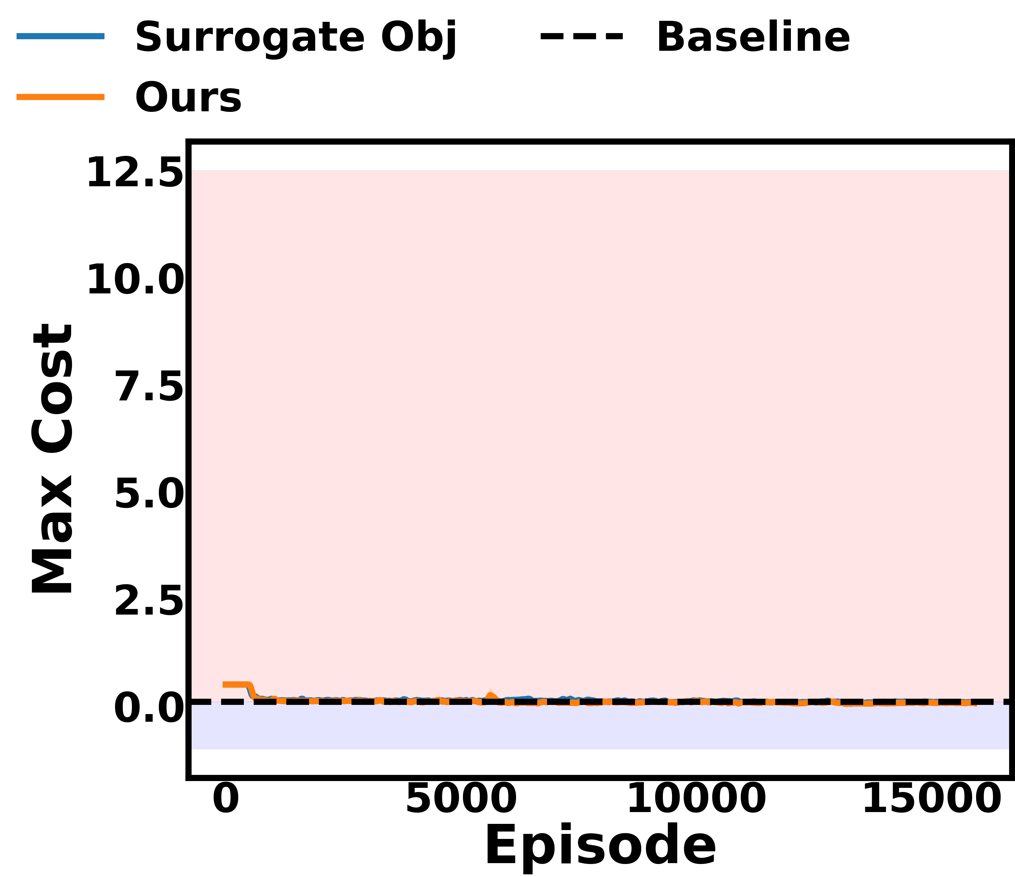
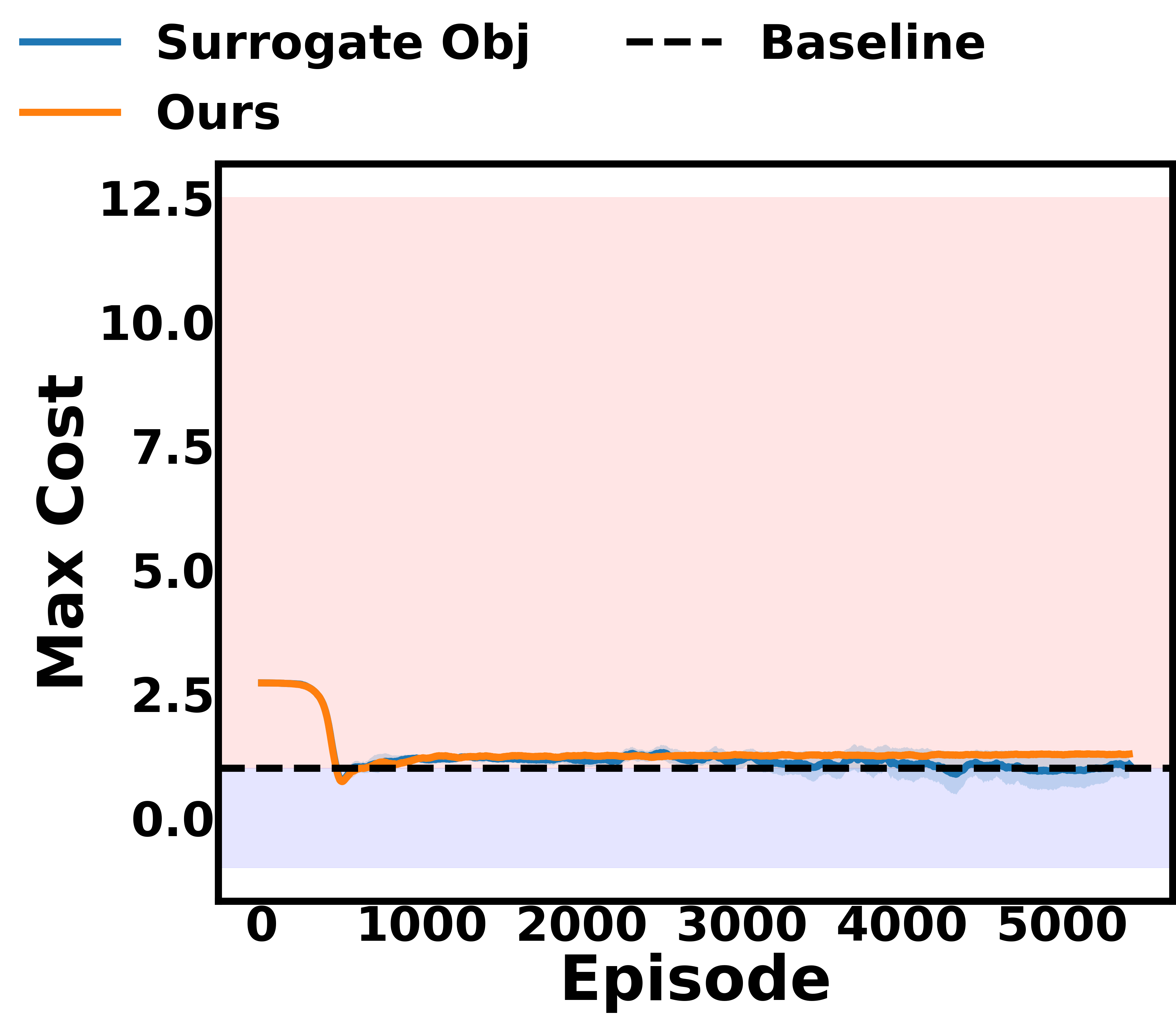
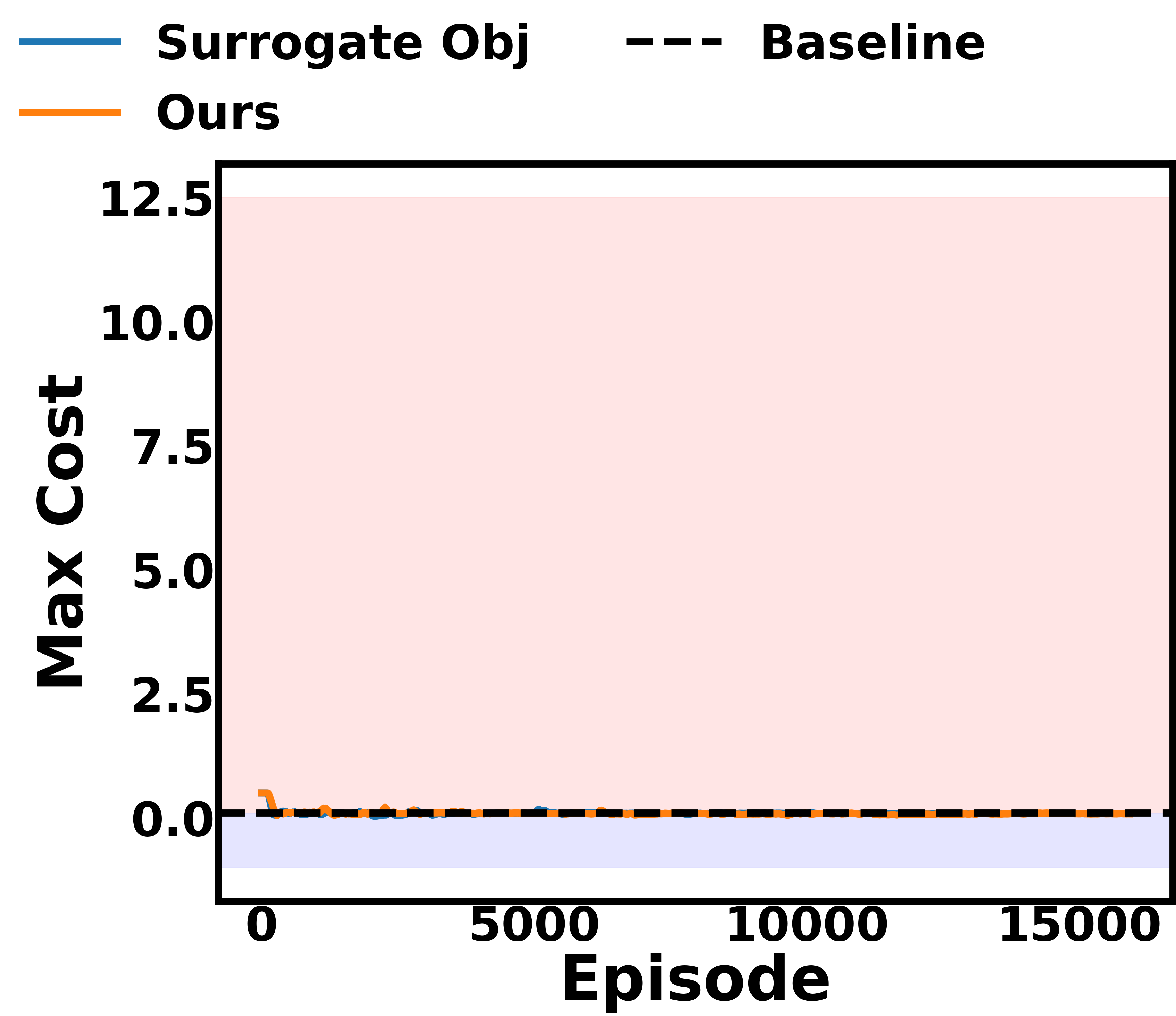
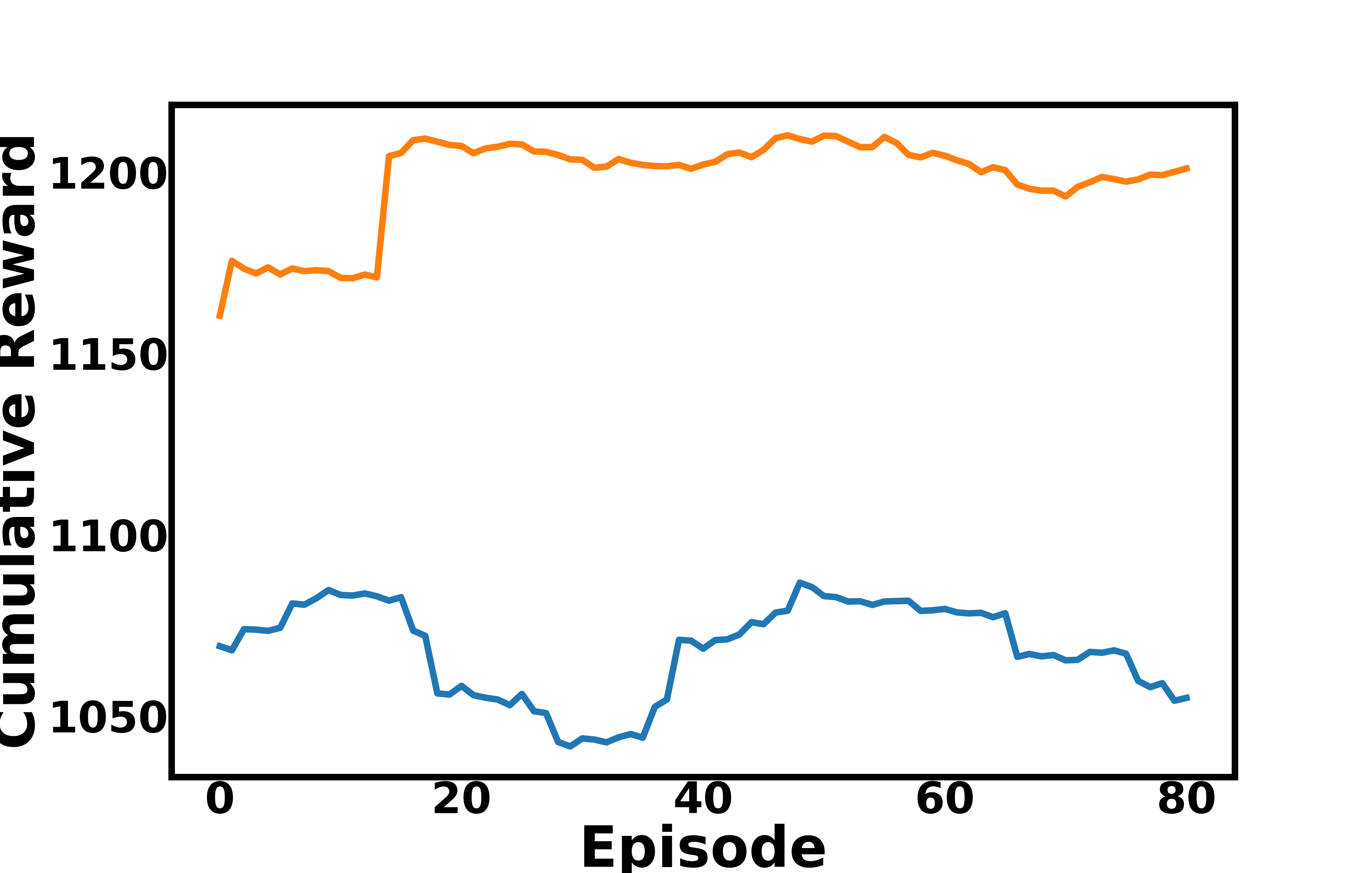
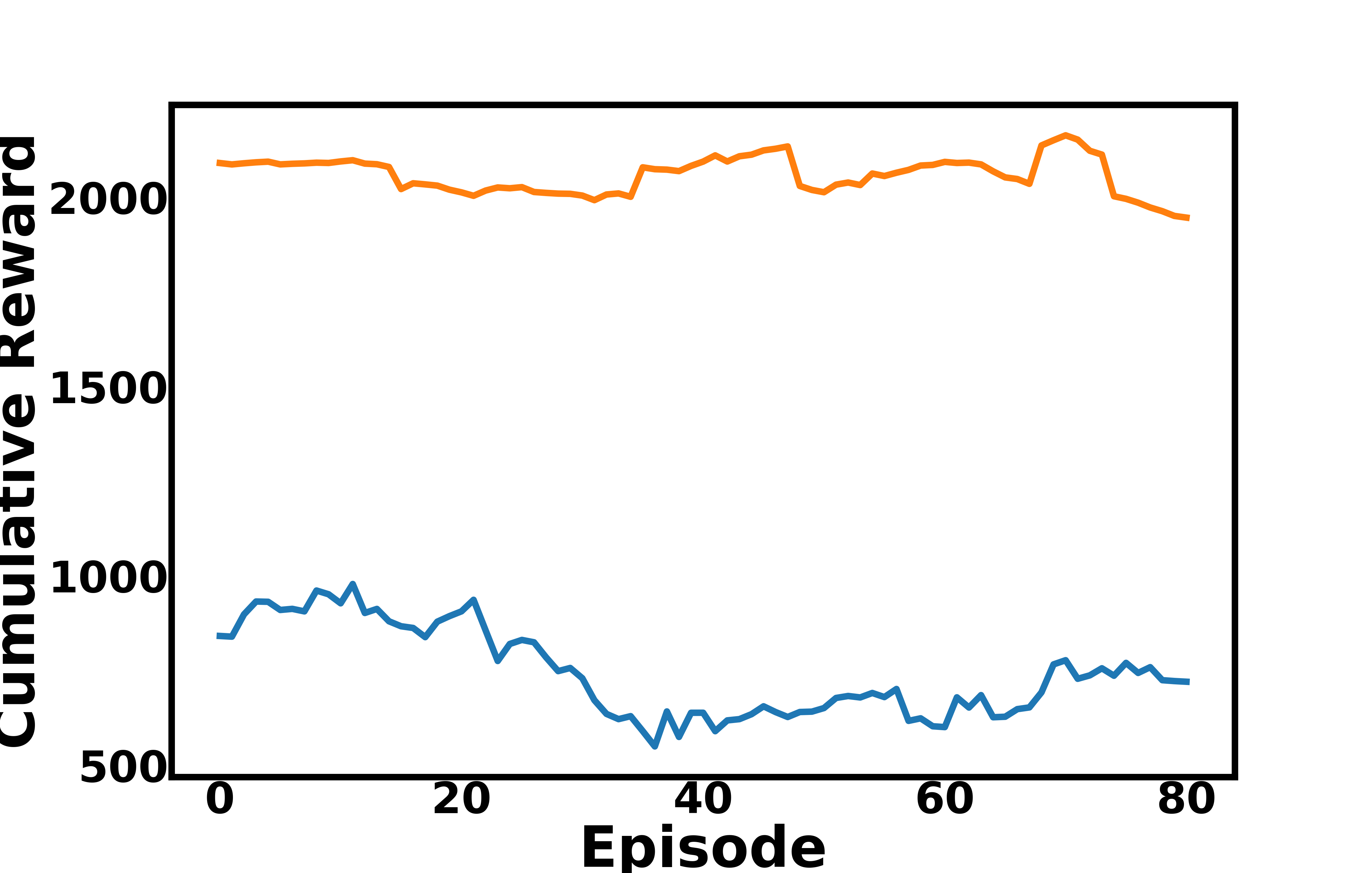
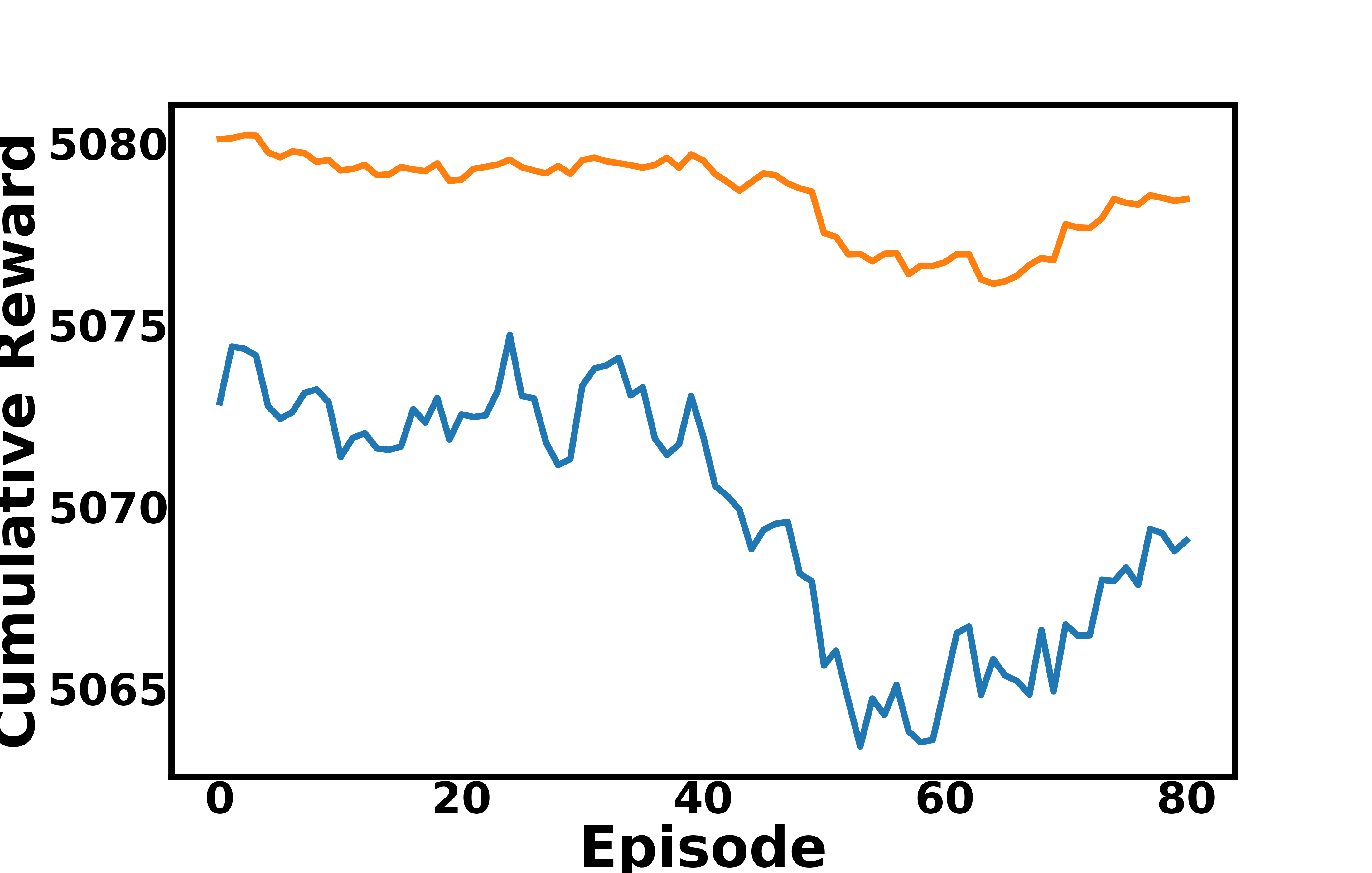
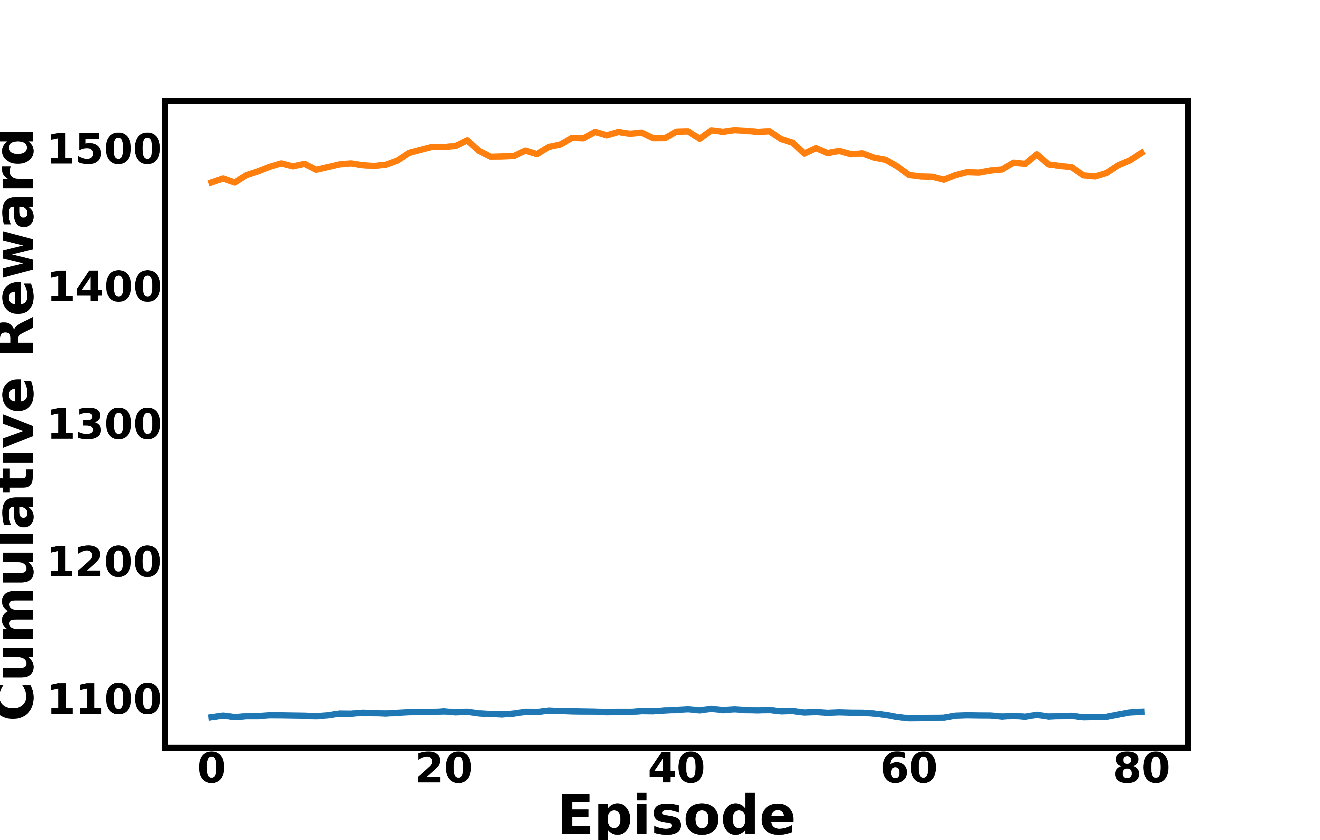
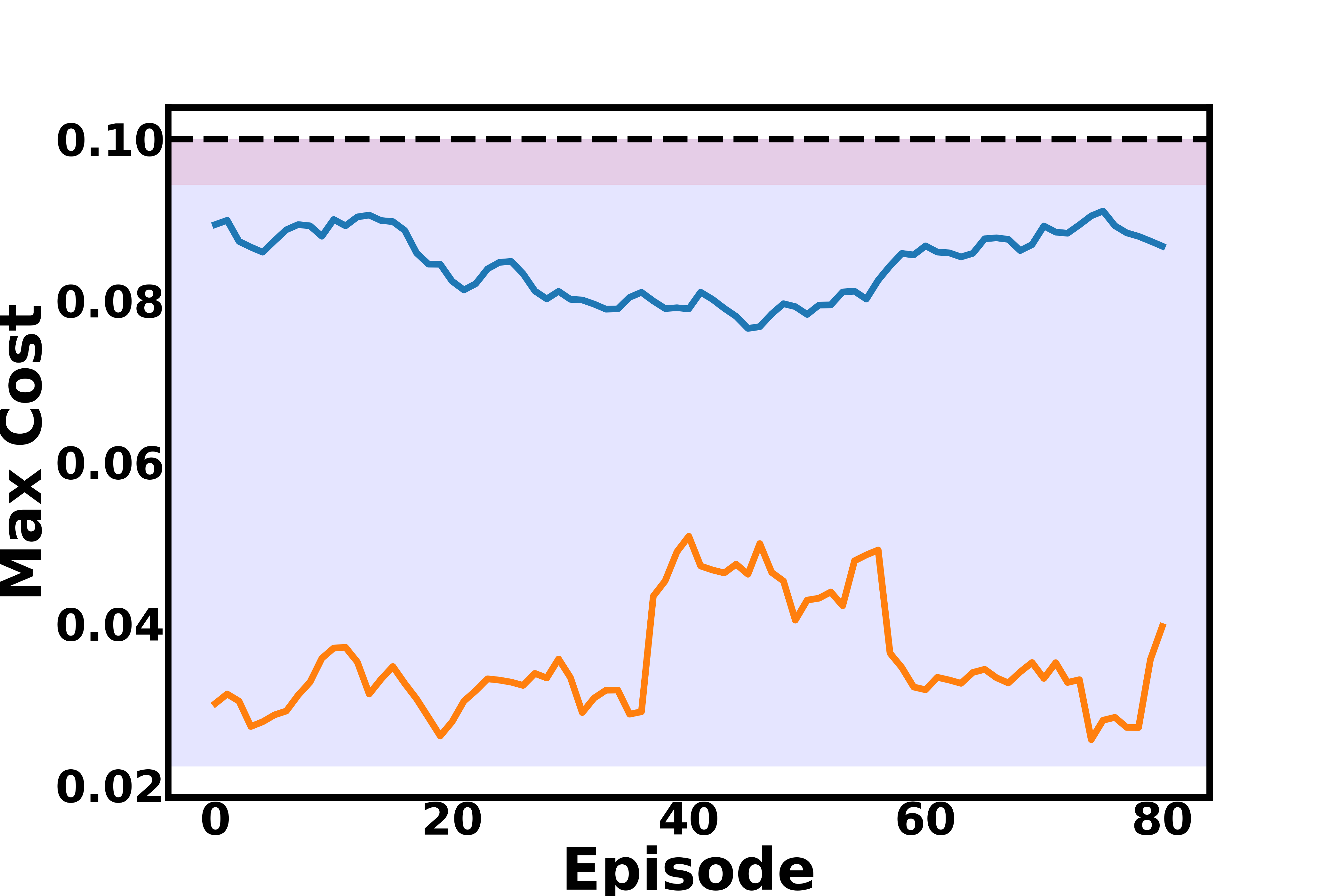
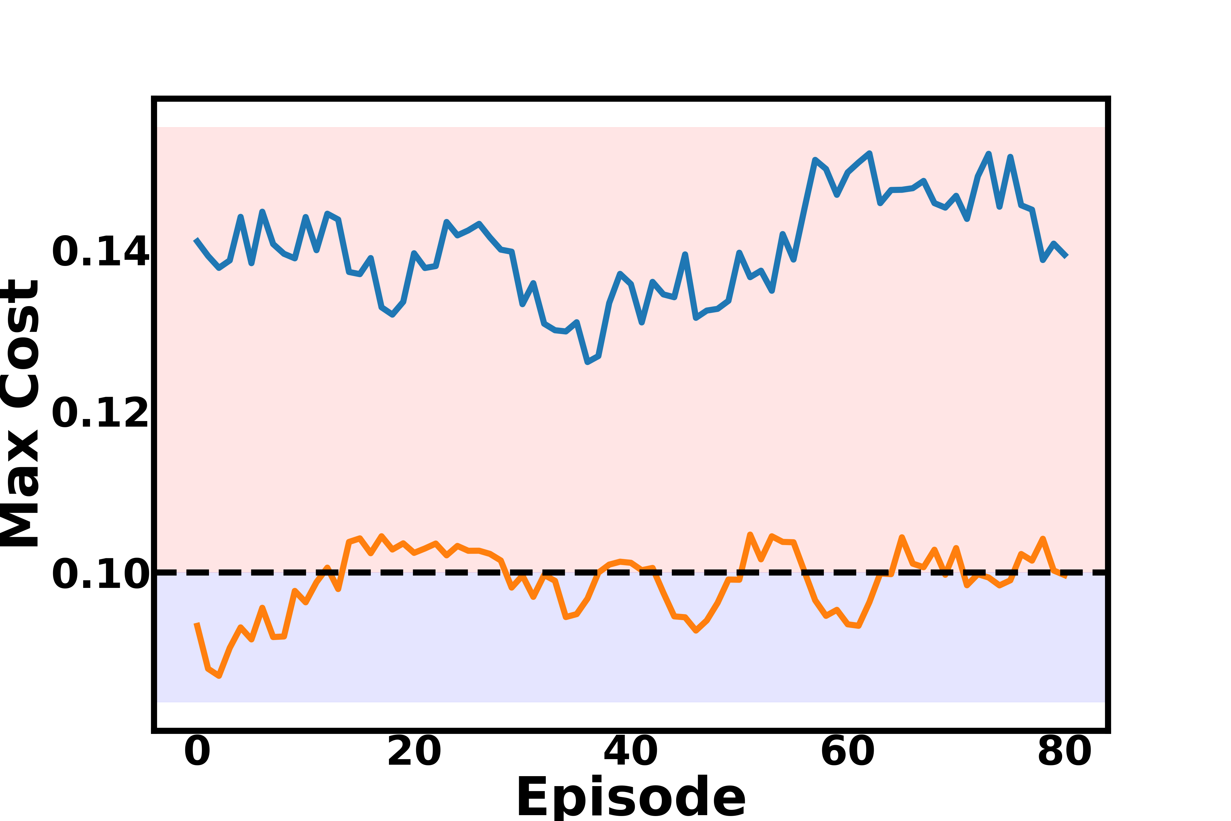
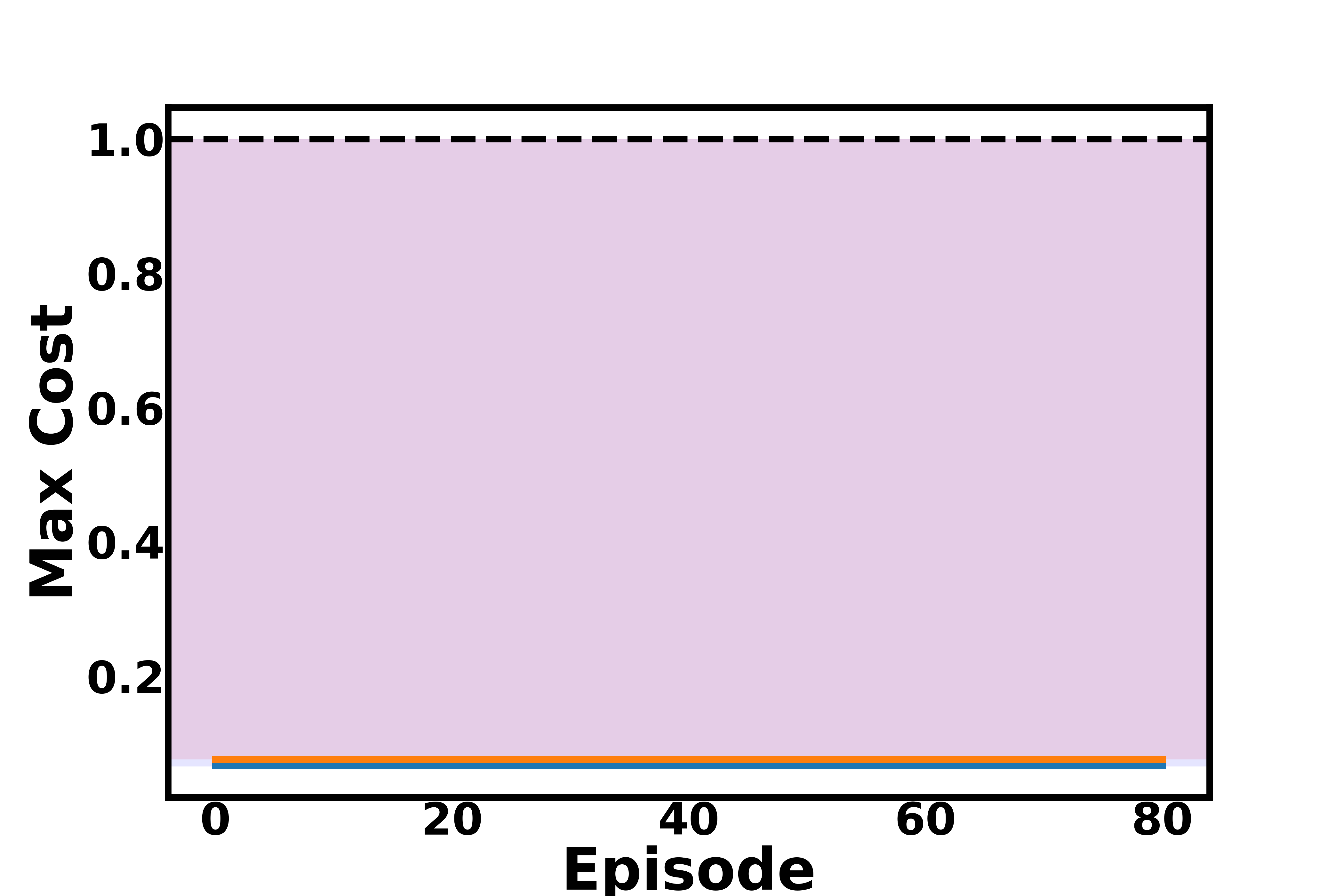
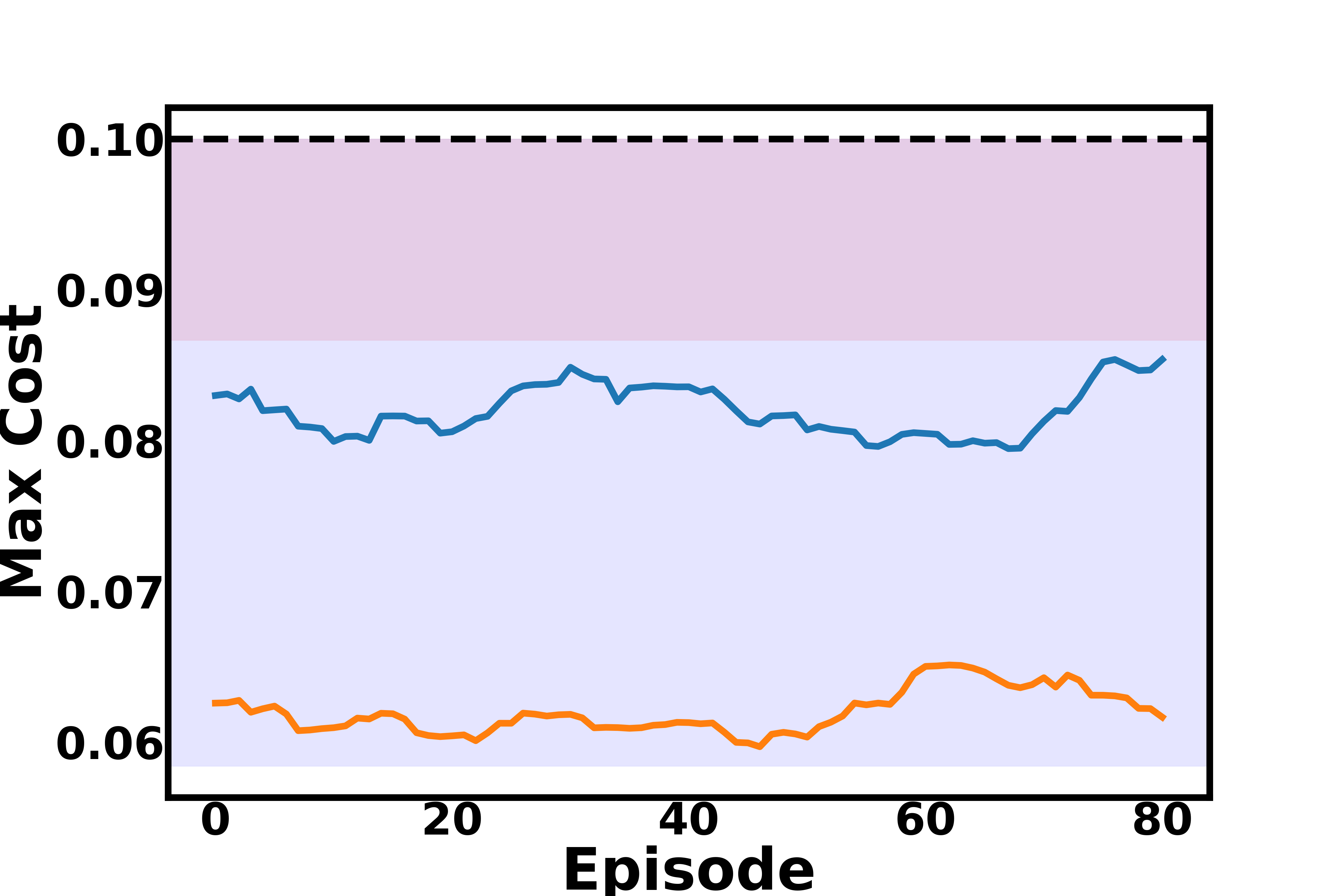

Figure 7: Training and inference performance across four MuJoCo environments. Rows show training returns, training maximum costs, inference returns, and inference maximum costs, respectively. We observe that RP-CRLhas better performance at perturbed inference, maintains persistent safety at perturbed inference, and the performance learning curve has lower standard deviation for RP-CRL..
We further evaluate RP-CRLon four MuJoCo environments: Ant, HalfCheetah, Humanoid, and Swimmer. For Ant, HalfCheetah, and Swimmer, the cost is defined using the maximum absolute action torque. The agent incurs zero cost when the maximum absolute action torque is below the threshold \(0.5\); otherwise, the cost is the amount by which this maximum torque exceeds \(0.5\). For Humanoid, the cost is defined as the energy consumption, computed as the sum of squared actions. During training, Ant and Humanoid are trained with gravity perturbations up to \(0.7\), HalfCheetah with gravity perturbations up to \(2.0\), and Swimmer with viscosity perturbations up to \(0.7\).
Fig. 7 compares the training behavior of RP-CRLwith the surrogate objective trained without robustness. During training, RP-CRLachieves smoother learning curves with lower variance while maintaining the peak-cost constraint more consistently across environments. This indicates that training under perturbed dynamics improves stability without sacrificing constraint satisfaction.
For inference, we evaluate the learned policies under stronger perturbations, with gravity perturbed up to \(2.0\) (Ant, HalfCheetah, Humanoid) and viscosity perturbed up to \(2.0\) (Swimmer). The inference results show that RP-CRLachieves better performance under perturbed dynamics and maintains persistent safety compared to the non-robust surrogate objective. These results demonstrate that robustness-aware training improves both return and safety generalization under environment uncertainty.
6 Conclusion and Future Work↩︎
In this work, we address the challenges of peak-cost constrained MDPs, demonstrating that they may not exhibit zero duality gap, unlike standard CMDPs. We propose a robust surrogate approach that achieves near-optimal solutions while ensuring constraint satisfaction within an acceptable margin \(b\). Through extensive experiments on a perturbed CartPole and Mujoco environments, we show that RP-CRLoutperforms existing methods in terms of both constraint satisfaction and reward optimization, even under uncertain dynamics. The characterization of the convergence guarantees of the proposed approach has been left for the future. Extending this framework to more complex real-world systems constitutes an important future research direction.
Acknowledgement↩︎
This work is partially supported by NSF ECCS Award #2534262.
6.1 Proof of Theorem 1and Proposition 1↩︎
Formal Statement of Theorem 1: Consider a discounted MDP with discount factor \(\gamma=0.9\), one nonterminal state \(s\), and one absorbing terminal state \(\bot\). At state \(s\), there are two actions:
action \(a_0\): reward \(r(s,a_0)=4\), cost \(c(s,a_0)=0\), and transition \[P(\bot\mid s,a_0)=1;\]
action \(a_1\): reward \(r(s,a_1)=8\), cost \(c(s,a_1)=\tfrac12\), and transition \[P(s\mid s,a_1)=1.\]
Let \(\pi_p\) denote the stationary randomized policy that chooses \(a_0\) with probability \(p\in[0,1]\) and \(a_1\) with probability \(1-p\). Define the hard-max modified constraint value \[\begin{align} V_c^{\pi_p}(s) = \sum_{a}\pi_p(a\mid s)\Bigl((1-\gamma)c(s,a) \nonumber\\ + \gamma \max\{c(s,a), \mathbb{E}[V_c^{\pi_p}(s')\mid s,a]\}\Bigr), \end{align}\] with \(V_c^{\pi_p}(\bot)=0\).
Consider the constrained optimization problem \[P^\star := \max_{p\in[0,1]} J_r(\pi_p) \qquad\text{s.t.}\qquad V_c^{\pi_p}(s)\le b,\] with threshold \(b=0.4\), where \(J_r(\pi_p)\) is the standard discounted reward value starting from \(s\). Here, note that peak cost-constraint across the trajectory is the same as here because of the two states with one state being terminal.
Then the associated Lagrangian dual \[D^\star := \inf_{\nu\ge 0}\;\sup_{p\in[0,1]} \Bigl\{ J_r(\pi_p)-\nu\bigl(V_c^{\pi_p}(s)-b\bigr) \Bigr\}\] satisfies \[D^\star>P^\star.\] More precisely, \[P^\star=\tfrac{180}{7}\approx 25.7143, \qquad D^\star=64.8,\] so that \[D^\star-P^\star=\tfrac{1368}{35}\approx 39.0857>0.\] Hence the peak-cost-constraint problem admits a strict duality gap.
Proof. Let \(J_r(\pi_p)\) denote the discounted reward value starting from \(s\). By the Bellman equation, \[J_r(\pi_p) = p\cdot 4 + (1-p)\bigl(8+\gamma J_r(\pi_p)\bigr).\] Since \(\gamma=0.9\), this becomes \[J_r(\pi_p) = 4p+(1-p)(8+0.9J_r(\pi_p)).\] Rearranging gives \[J_r(\pi_p)\bigl(1-0.9(1-p)\bigr)=8-4p,\] hence \[J_r(\pi_p)=\tfrac{8-4p}{0.1+0.9p}.\]
Next, let \(V(p):=V_c^{\pi_p}(s)\). By definition of the modified hard-max constraint, \[\begin{align} V(p) &= p\Bigl((1-\gamma)\cdot 0+\gamma\max\{0,0\}\Bigr) + \notag\\ & \qquad (1-p)\Bigl((1-\gamma)\tfrac12 +\gamma\max\{\tfrac12,V(p)\}\Bigr). \end{align}\] The first term is zero, so \[V(p) = (1-p)\Bigl(0.1\cdot\tfrac12+0.9\max\{\tfrac12,V(p)\}\Bigr).\]
We now solve this fixed-point equation. Suppose first that \(V(p)\le \tfrac12\). Then \[\max\{\tfrac12,V(p)\}=\tfrac12,\] and thus \[V(p) = (1-p)\Bigl(0.05+0.9\cdot\tfrac12\Bigr) = (1-p)\cdot\tfrac12 = \tfrac{1-p}{2}.\] Since \(\tfrac{1-p}{2}\le \tfrac12\) for all \(p\in[0,1]\), this is self-consistent. Therefore, \[V_c^{\pi_p}(s)=\tfrac{1-p}{2},\qquad \forall p\in[0,1].\]
We now solve the primal problem \[\max_{p\in[0,1]} J_r(\pi_p) \qquad\text{s.t.}\qquad \tfrac{1-p}{2}\le 0.4.\] The constraint is equivalent to \[1-p\le 0.8 \iff p\ge 0.2.\] Moreover, \[J_r(\pi_p)=\tfrac{8-4p}{0.1+0.9p},\] and differentiating yields \[\begin{align} \tfrac{d}{dp}J_r(\pi_p) = \tfrac{-4(0.1+0.9p)-(8-4p)(0.9)}{(0.1+0.9p)^2} \nonumber \\ = \tfrac{-7.6}{(0.1+0.9p)^2}<0. \end{align}\] Hence \(J_r(\pi_p)\) is strictly decreasing in \(p\), so the primal optimum is attained at the smallest feasible \(p\), namely \(p^\star=0.2\). Therefore, \[P^\star = J_r(\pi_{0.2}) = \tfrac{8-4(0.2)}{0.1+0.9(0.2)} = \tfrac{7.2}{0.28} = \tfrac{180}{7}.\]
Now consider the Lagrangian \[L(p,\nu) = J_r(\pi_p)-\nu\bigl(V_c^{\pi_p}(s)-0.4\bigr), \qquad \nu\ge 0.\] Substituting the formulas for \(J_r(\pi_p)\) and \(V_c^{\pi_p}(s)\) gives \[\begin{align} L(p,\nu) = \tfrac{8-4p}{0.1+0.9p} - \nu\left(\tfrac{1-p}{2}-0.4\right) \nonumber \\ = \tfrac{8-4p}{0.1+0.9p} -\nu(0.1-0.5p). \end{align}\]
Fix \(\nu\ge 0\). The derivative with respect to \(p\) is \[\tfrac{\partial}{\partial p}L(p,\nu) = -\tfrac{7.6}{(0.1+0.9p)^2} +\tfrac{\nu}{2},\] and the second derivative is \[\tfrac{\partial^2}{\partial p^2}L(p,\nu) = \tfrac{13.68}{(0.1+0.9p)^3}>0.\] Thus for every fixed \(\nu\), the function \(p\mapsto L(p,\nu)\) is convex on \([0,1]\). Therefore its supremum over \([0,1]\) is attained at one of the endpoints: \[g(\nu) := \sup_{p\in[0,1]}L(p,\nu) = \max\{L(0,\nu),L(1,\nu)\}.\]
Evaluating the endpoints, \[L(0,\nu)=\tfrac{8}{0.1}-0.1\nu=80-0.1\nu,\] and \[L(1,\nu)=\tfrac{4}{1}+0.4\nu=4+0.4\nu.\] Hence \[g(\nu)=\max\{80-0.1\nu,\;4+0.4\nu\}.\]
The minimum of this maximum of two affine functions occurs when they are equal: \[80-0.1\nu=4+0.4\nu \iff 76=0.5\nu \iff \nu^\star=152.\] Substituting back, \[D^\star=g(\nu^\star)=80-0.1(152)=64.8.\]
Finally, \[\begin{align} D^\star-P^\star = 64.8-\tfrac{180}{7} = \tfrac{324}{5}-\tfrac{180}{7} & = \tfrac{2268-900}{35} \\ &= \tfrac{1368}{35} >0. \end{align}\] Thus the duality gap is strict. ◻
Proof of Proposition 1:
Proof. Part (i): Reward Optimality. Since \(\pi^*\) is feasible for problem 5 , we have: \(\max_{P \in \mathcal{P},\;s \in \mathcal{S}^{\pi^*}} V_{c,\mathrm{peak}}^{\pi^*,P}(s) \leq b,\) which implies: the surrogate objective evaluated at \(\pi^*\) satisfies: \[\begin{align} & \max\left\{\frac{\max_{P \in \mathcal{P}} J_r^{\pi^*,P}}{\beta},\; \max_{P \in \mathcal{P},\;s \in \mathcal{S}^{\pi^*}} V_{c,\mathrm{peak}}^{\pi^*,P}(s) - b\right\} \nonumber\\ & = \frac{\max_{P \in \mathcal{P}} J_r^{\pi^*,P}}{\beta}, \end{align}\] since the second term inside the max is non-positive. Since \(\hat{\pi}^*\) is the minimizer of the surrogate problem 7 , we have: \[\begin{align} & \max\left\{\frac{\max_{P \in \mathcal{P}} J_r^{\hat{\pi}^*,P}}{\beta},\; \max_{P \in \mathcal{P},\;s \in \mathcal{S}^{\hat{\pi}^*}} V_{c,\mathrm{peak}}^{\hat{\pi}^*,P}(s) - b\right\} \nonumber\\& \geq \frac{\max_{P \in \mathcal{P}} J_r^{\pi^*,P}}{\beta}. \end{align}\] Since the left-hand side is greater than or equal to \(\frac{\max_{P \in \mathcal{P}} J_r^{\hat{\pi}^*,P}}{\beta}\), the result follows for the minimization objective.
Part (ii): Constraint Violation Bound. From the optimality of \(\hat{\pi}^*\) and the bound established in Part (i): \[\begin{align} & \max\left\{\frac{\max_{P \in \mathcal{P}} J_r^{\hat{\pi}^*,P}}{\beta},\; \max_{P \in \mathcal{P},\;s \in \mathcal{S}^{\hat{\pi}^*}} V_{c,\mathrm{peak}}^{\hat{\pi}^*,P}(s) - b\right\} \nonumber\\ & \geq \frac{\max_{P \in \mathcal{P}} J_r^{\pi^*,P}}{\beta}. \end{align}\] In particular, the second term inside the max satisfies: \[\max_{P \in \mathcal{P},\;s \in \mathcal{S}^{\hat{\pi}^*}} V_{c,\mathrm{peak}}^{\hat{\pi}^*,P}(s) - b \geq \frac{\max_{P \in \mathcal{P}} J_r^{\pi^*,P}}{\beta}.\] Let us consider the cost values \(c_i \in [0,C_\text{max}]\). Since \(V_{c,\mathrm{peak}}^{\pi,P}(s) \in [0, C_\text{max}]\) for all \(\pi, P, s\) by definition of the peak-cost value function, and \(J_r^{\pi^*,P} \leq C_{max}\), we obtain: \[\max_{P \in \mathcal{P},\;s \in \mathcal{S}^{\hat{\pi}^*}} V_{c,\mathrm{peak}}^{\hat{\pi}^*,P}(s) - b \leq \frac{C_\text{max}}{\beta}.\] Setting \(\beta \geq C_\text{max}/\epsilon\) completes the proof of part (ii). ◻
References↩︎
\(^{1}\)Dept. of Electrical and Computer Engineering, NJIT, Newark, NJ, USA
(E-mails: {sm3934,sg2786,arnob.ghosh}@njit.edu)↩︎\(^{2}\)School of Electrical Engineering and Computer Science Washington State University, Pullman, WA, USA
(E-mail: honghao.wei@wsu.edu)↩︎\(^{3}\) Department of Mechanical and Aerospace Engineering, The Ohio State University, Columbus, OH, USA
(E-mail: {rajkumar.36,goswami.78}@osu.edu)↩︎