Design-Based Supervised Learning
with Noisy Human Labels
July 16, 2026
Abstract
Researchers increasingly use automated classifiers to label unstructured data for statistical analysis. Existing rectification methods can correct errors in these automated labels using a probability-sampled audit set, but they usually treat the audit labels as correct. In practice, human audit labels are often noisy, and only some audited items are reviewed by an expert or adjudicator. We propose Partially Adjudicated Design-Based Supervised Learning (PA-DSL), a method for this setting. It uses adjudicated cases to correct noisy human labels and then uses the corrected audit information to debias analyses based on the full set of automated labels. The estimator is valid for a broad class of downstream analyses when the audit and adjudication probabilities are known. In synthetic and Wikipedia Detox semi-synthetic experiments, PA-DSL maintains nominal coverage and reduces RMSE by 10–17% relative to using only adjudicated labels when noisy human labels contain recoverable signal.
1 Introduction↩︎
Empirical research in the social sciences, business, law, and related fields often depends on coding raw texts, images, or records into variables that measure substantive constructs [1], [2]. Traditionally, this coding has relied on human or expert judgment, making it costly, time-consuming, and prone to inconsistency. Automated classifiers now make it possible to code data at scale, ranging from traditional supervised text classifiers to newer LLM-based systems [3]–[5]. But classifier-generated labels are noisy measurements, not observed outcomes [6]. Systematic prediction errors can bias downstream estimates and produce undercovered confidence intervals, even when classifiers achieve high overall accuracy [7].
This has motivated a growing set of rectification methods that use higher-quality validation or audit data to correct estimates based on full-population surrogate labels [6], [8]–[11]. The common structure is simple: inexpensive automated labels provide scale, while a smaller set of trusted labels anchors the correction. Design-Based Supervised Learning (DSL), for example, combines a full-population surrogate score with a probability-sampled audit to obtain valid inference for downstream estimands such as regression coefficients [10].
In many real labeling pipelines, however, the audit labels used for correction are not themselves gold standard. Human annotators disagree, and disagreement often reflects ambiguity, subjectivity, or guideline interpretation rather than only random coder error [12]–[14]. Because expert reconciliation is costly [15], [16], a common workflow is to have one or more human annotators label all items from an “audited” sample, with only selected items from it receiving expert adjudication. This multi-reviewer or adjudication design is widespread, reappearing across domains diverse as content analysis, systematic reviews, clinical endpoint assessment, and NLP annotation [17]–[20]. Existing rectification strategies do not fully address this setting because the audit used to correct the surrogate may itself be measured with error.
This paper introduces Partially Adjudicated Design-Based Supervised Learning (PA-DSL), a design-based estimator for downstream inference under hierarchical label noise. Conceptually, PA-DSL is not a new estimating principle from scratch, but a nested application of known-probability AIPW/DSL corrections to a partially adjudicated annotation design. It uses an inner correction to turn the adjudicated subset into audit-level pseudo-labels, and an outer correction to use those pseudo-labels to debias inference based on the full-population surrogate. To our knowledge, this is the first work to extend rectification methods beyond the usual gold-audit setting, allowing the human audit labels used for correction to be noisy and only partially adjudicated.
1.0.0.1 Contributions.
The paper makes three contributions. First, it formalizes a three-tier nested measurement design with noisy audit labels and partial adjudication. Second, it proves that the resulting pseudo-outcome is design-valid for any downstream estimating equation affine in the latent outcome, provided the audit and adjudication probabilities are known by design. Third, it shows in synthetic and semi-synthetic experiments that PA-DSL retains the coverage of adjudication-only DSL while improving efficiency when the noisy audit labels contain recoverable information about the adjudicated construct.
2 Setup: Hierarchical Label Noise and Target Estimand↩︎
2.0.0.1 Observed data.
We observe an i.i.d.sample of size \(N\), where each unit \(i\) contributes \[W_i \;=\; \bigl(\boldsymbol{X}_i,\, Q_i,\, R_i,\, G_{i,1},\, G_{i,2},\, V_i,\, A_i\bigr),\] generated jointly with a latent binary truth \(Y^{\star}_i \in \{0,1\}\) that the analyst does not observe. Here \(\boldsymbol{X}_i \in \mathbb{R}^{p+1}\) is a covariate vector with leading intercept; \(Q_i \in [0,1]\) is a real-valued surrogate score; \(R_i \in \{0,1\}\) is the audit indicator with known sampling probability \(\pi_i \in (0,1)\); \(G_{i,1}, G_{i,2} \in \{0,1\}\) are two human coder labels observed iff \(R_i = 1\); \(V_i \in \{0,1\}\) is the adjudication indicator with known probability \(\rho_i \equiv \mathbb{P}(V_i = 1 \mid R_i = 1, Z_i) \in (0,1)\) a known function of the inner features defined just below; and \(A_i \in \{0,1\}\) is the adjudicated label, observed iff \(R_i V_i = 1\). The score \(Q_i\) need not be calibrated; it is treated as an observed surrogate feature whose systematic errors are corrected by the audit design. We write \(B_i = (Q_i, \boldsymbol{X}_i^\top)^\top\) for the outer feature vector and \(Z_i = (Q_i, \boldsymbol{X}_i^\top, G_{i,1}, G_{i,2})^\top\) for the inner feature vector. We use two coder labels as the running case because this is a common annotation workflow and makes disagreement-based adjudication easy to describe. However, the construction does not require exactly two labels: more generally, \(Z_i\) may contain any audit-tier information observed when \(R_i=1\), including \(K_i\) coder labels, coder identities, agreement indicators, vote shares, uncertainty scores, item metadata, or other features used in the adjudication design. The probabilities \(\pi_i\) and \(\rho_i\) are design parameters chosen by the researcher, so they are known, not estimated.
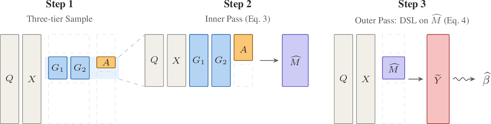
1 summarizes the nested three-tier sampling design. Throughout, the tiers refer to nested measurement availability, not mutually exclusive samples. Tier 1 contains all \(N\) units and includes \((X_i,Q_i)\). Tier 2 is the audit subset \(\{i:R_i=1\}\), which also includes noisy coder labels \((G_{i1},G_{i2})\). Tier 3 is the adjudicated subset \(\{i:R_iV_i=1\}\), which also includes the adjudicated label \(A_i\). Hence tier 3 \(\subset\) tier 2 \(\subset\) tier 1.
2.0.0.2 Target estimand.
In the applications motivating this paper, the scientific target is often not whether each individual text or record is classified correctly, but how a target construct varies across groups, treatments, or covariates. For subjective annotation tasks, we interpret \(Y^{\star}_i\) as the label that would be assigned to unit \(i\) under the target adjudication protocol, rather than as an externally verified objective truth. We therefore target a population-level regression summary for this adjudication-defined construct: the logistic projection of \(Y^{\star}_i\) onto the covariates. Formally, we focus on the parameter \(\beta \in \mathbb{R}^{p+1}\) defined as the unique solution of the population score equation \[\mathbb{E}\bigl[\boldsymbol{X}_i\,\bigl(Y^{\star}_i - \operatorname{expit}(\boldsymbol{X}_i^\top \beta)\bigr)\bigr] \;=\; \mathbf{0}, \label{eq:beta-pop}\tag{1}\] reporting the slope \(\beta_1\) on the first non-intercept covariate. This is the logistic-regression M-estimand for \(Y^{\star}\) given \(\boldsymbol{X}\). Validity for an objective construct beyond the protocol-defined target requires the additional measurement-validity assumption that the adjudication protocol itself captures that construct.
The working model serves only as a specification choice for the score equation; it has a literal conditional-probability interpretation if and only if it holds exactly, which we do not assume. 1 is outcome-affine: the score is linear in \(Y^{\star}_i\) for any fixed \(\beta\). The construction in Section 3 produces an unbiased pseudo-outcome \(\widetilde{Y}_i\) for \(Y^{\star}_i\), so any outcome-affine estimating equation (the population mean, generalized linear regression, inverse-propensity weighted treatment effects, etc.) can be solved by substituting \(\widetilde{Y}_i\) for \(Y^{\star}_i\). We treat the population prevalence \(\mathbb{E}[Y^{\star}]\) as the special case in which the score is \(Y^{\star}_i - \psi\); see 7 for that variant and its empirical results.
Importantly, we do not assume that \(Q_i\) is calibrated, unbiased, or a consistent estimator of \(Y_i^\star\). The surrogate score is treated as an observed feature available on the full frame. Its systematic errors are corrected by the audit/adjudication design, as in standard DSL. Identification comes from the known audit and adjudication probabilities together with the ignorability/correctness assumptions below, not from any correctness property of \(Q_i\). The quality of \(Q_i\) affects efficiency through the nuisance functions, but not design validity.
2.0.0.3 Identifying assumptions.
The audit/adjudication design supplies four assumptions; together they identify the population means we will need.
Assumption 1 (Audit ignorability). \(R_i \perp\!\!\!\perp Y^{\star}_i \mid (\boldsymbol{X}_i, Q_i)\), with \(\pi_i\) bounded away from \(0\) and \(1\). Holds by construction whenever audit assignment is a randomized function of observed design variables.
Assumption 2 (Adjudication ignorability). \(V_i \perp\!\!\!\perp Y^{\star}_i \mid (R_i = 1, Z_i)\), with \(\rho_i\) bounded away from \(0\) and \(1\). Holds whenever adjudication is randomized with known probability as a known function of \(Z_i\) — for example, high-probability adjudication on coder disagreement and lower but nonzero adjudication on agreement cases. Strictly deterministic prioritization rules require an additional positive sampling floor in every design stratum used for inference (14 sweeps this floor).
Assumption 3 (Protocol-level Adjudication correctness). On adjudicated units, \(A_i=Y_i^\star\), where \(Y_i^\star\) denotes the label that would be assigned under the target adjudication protocol.
Assumption 4 (Coder labels are observed noisy features). The coder labels \((G_{i,1},G_{i,2})\) and any other audit-tier metadata included in \(Z_i\) are observed on the audit set and may be arbitrary noisy functions of the latent truth, item difficulty, coder identity, task context, or other factors. We do not require coder independence, unbiasedness, a fixed number of coders, or a parametric coder-error model.
Assumption 4 is a measurement condition rather than an identifying model: All audit-tier information, including \((G_{i,1},G_{i,2})\), enter only as observed features in \(Z_i\). Their bias, dependence, and heterogeneity are absorbed into \(\mu_0(Z_i)\); design validity comes from the known adjudication probability \(\rho_i\) and adjudication correctness.
3 Estimator: Partially Adjudicated DSL↩︎
Standard DSL [10] replaces the unobserved \(Y^{\star}_i\) with a pseudo-outcome of the form \(\hat{g}(B_i) + (R_i / \pi_i)\bigl(Y_i^{\text{gold}} - \hat{g}(B_i)\bigr)\), where \(\hat{g}\) is a cross-fit nuisance regression of the gold label on \(B_i\) and the Horvitz–Thompson correction debiases that regression at the known audit weight. The construction assumes \(Y_i^{\text{gold}} = Y^{\star}_i\) on the audit set; when the audit labels are themselves noisy, substituting any one of \(G_{i,1}\), \(G_{i,2}\), or their majority vote inherits the human bias. We address this by nesting a second design-based correction inside, exploiting the fact that the adjudicated label \(A_i\) is unbiased for \(Y^{\star}_i\) on \(\{R_i V_i = 1\}\) with known sampling weight \(\rho_i\).
3.0.0.1 Step 1 — Inner correction.
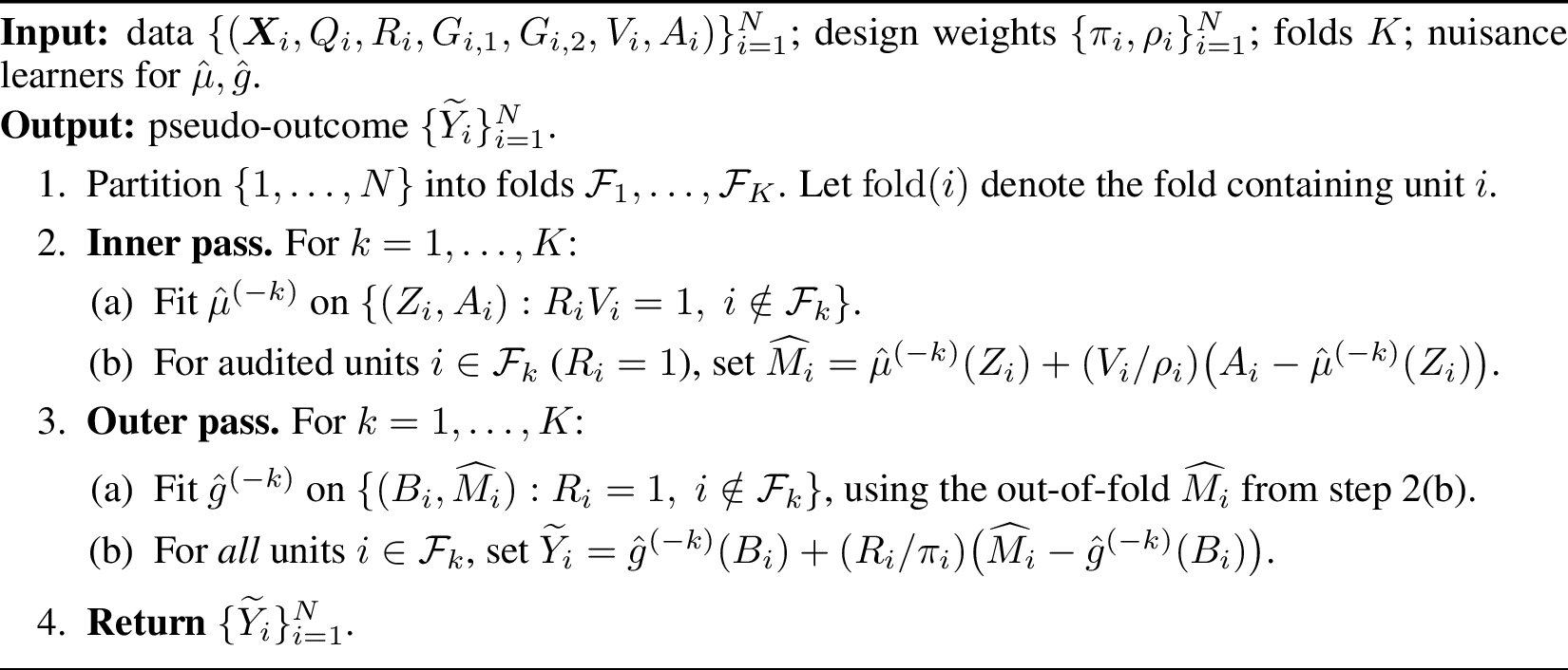
Given any cross-fit estimator \(\hat{\mu}(\cdot)\) of the inner nuisance \(\mu_0(z) = \mathbb{E}[A_i \mid Z_i = z, R_i = 1, V_i = 1]\) trained on the adjudicated subset \(\{R_i V_i = 1\}\), define the audit-level pseudo-label \[\widehat M_i \;=\; \hat{\mu}(Z_i) \;+\; \frac{V_i}{\rho_i}\,\bigl(A_i - \hat{\mu}(Z_i)\bigr), \qquad i \in \{R_i = 1\}. \label{eq:Mhat}\tag{2}\] Here \(\hat{\mu}(Z_i)\) uses the surrogate, the covariates, and the two coder labels to predict adjudicated truth, and the \(V_i/\rho_i\) term debiases that prediction on the adjudicated subset. This definition is unchanged if \(Z_i\) contains more than two coder labels or additional audit-tier metadata; the inner correction only requires that the adjudication probability \(\rho_i=P(V_i=1\mid R_i=1,Z_i)\) be known by design and bounded away from zero.
3.0.0.2 Step 2 — Outer correction.
Given a cross-fit estimator \(\hat{g}(\cdot)\) of the outer nuisance \(g_0(b) = \mathbb{E}\{\mu_0(Z_i)\mid B_i=b,R_i=1\}\) trained on the audit set \(\{R_i = 1\}\) using \(\widehat M_i\) as response, define the final pseudo-outcome \[\widetilde{Y}_i \;=\; \hat{g}(B_i) \;+\; \frac{R_i}{\pi_i}\,\bigl(\widehat M_i - \hat{g}(B_i)\bigr), \qquad i = 1, \dots, N. \label{eq:Ytilde}\tag{3}\] Under Assumptions 1–3, this target satisfies \(g_0(B_i)=\mathbb{E}(Y_i^\star\mid B_i)\); the realized pseudo-label \(\widehat M_i\) is used only to estimate this population nuisance.
Substituting 2 into 3 gives the closed form below, which makes the three roles transparent \[\boxed{\; \widetilde{Y}_i \;=\; \underbrace{\hat{g}(B_i)}_{\text{full-frame regression}} \;+\; \underbrace{\frac{R_i}{\pi_i}\,\bigl[\hat{\mu}(Z_i) - \hat{g}(B_i)\bigr]}_{\text{audit correction}} \;+\; \underbrace{\frac{R_i V_i}{\pi_i \rho_i}\,\bigl[A_i - \hat{\mu}(Z_i)\bigr]}_{\text{adjudication correction}} \;} \label{eq:Ytilde-expanded}\tag{4}\]
Thus, PA-DSL uses adjudication only to correct the part of the audit information that cannot be trusted, while still allowing the unadjudicated human labels to improve efficiency through \(\hat{\mu}(Z_i)\).
3.0.0.3 Step 3 — Downstream estimating equation.
Substitute \(\widetilde{Y}_i\) for \(Y^{\star}_i\) in the population score 1 and solve the empirical analog: \[\frac{1}{N} \sum_{i=1}^{N} \boldsymbol{X}_i\,\bigl(\widetilde{Y}_i - \operatorname{expit}(\boldsymbol{X}_i^\top \hat{\beta})\bigr) \;=\; \mathbf{0}, \label{eq:beta-emp}\tag{5}\] returning the cross-fit estimator \(\hat{\beta}\). Standard errors come from the sandwich formula evaluated at \((\boldsymbol{X}_i, \widetilde{Y}_i)\).
3.0.0.4 Why \(\widetilde{Y}_i\) is design-valid.
Both corrections in 2 3 are AIPW-style augmentations [21] with known design weights. Under , iterated expectations give \(\mathbb{E}[\widehat M_i\mid R_i=1,Z_i]=\mathbb{E}[Y^{\star}_i\mid R_i=1,Z_i]\) and \(\mathbb{E}[\widetilde{Y}_i\mid B_i]=\mathbb{E}[Y^{\star}_i\mid B_i]\), regardless of nuisance specification. Thus the nuisances affect efficiency, not design validity; full algebra and influence functions are in 8.
3.0.0.5 Cross-fitting.
Algorithm 2 uses a shared fold partition for the inner and outer passes, which is the implementation used in the experiments. For the cleanest theoretical argument, Appendix 8 first analyzes a leakage-free nested variant in which the outer nuisance for a held-out fold is trained using audit pseudo-labels constructed without any information from that fold. The shared-partition version differs only through an indirect dependence of the outer nuisance on the held-out fold through the inner pseudo-labels used in outer training. Appendix 8 isolates this difference as a stability remainder and states the high-level condition under which the shared-partition implementation has the same first-order expansion.
Write \(m(W_i; \beta, \eta) = \boldsymbol{X}_i\,(\widetilde{Y}_i(\eta) - \operatorname{expit}(\boldsymbol{X}_i^\top \beta))\) for the estimating function, with \(\eta = (\mu, g)\) now an explicit argument, and let \(\beta_0\) denote the population value of \(\beta\) defined by 1 .
Proposition 1 (Design validity and asymptotic normality). Suppose hold, the design weights \(\pi_i,\rho_i\) are known and bounded away from zero and one, \(\mathbb{E}\|\boldsymbol{X}_i\|^{2+\delta}<\infty\) for some \(\delta>0\), and \[\mathbf{H} = \mathbb{E}\!\left[ \boldsymbol{X}_i\boldsymbol{X}_i^\top \operatorname{expit}'\!\left(\boldsymbol{X}_i^\top\beta_0\right) \right]\] is nonsingular. For the leakage-free nested cross-fit estimator, under cross-fit \(L^2\)-consistent nuisance estimation, \(\hat{\beta}\) defined by 5 satisfies \[\sqrt N(\hat{\beta}-\beta_0) = \mathbf{H}^{-1} \frac{1}{\sqrt N}\sum_{i=1}^N m(W_i;\beta_0,\eta_0) + o_p(1),\] and hence \[\sqrt N(\hat{\beta}-\beta_0) \rightsquigarrow \mathcal{N}\!\left( \mathbf{0},\, \mathbf{H}^{-1}\Omega \mathbf{H}^{-1\top} \right),\] where \[\Omega = \mathbb{E}\!\left[ m(W_i;\beta_0,\eta_0)m(W_i;\beta_0,\eta_0)^\top \right] = \operatorname{Var}\{m(W_i;\beta_0,\eta_0)\}, \qquad \eta_0=(\mu_0,g_0).\] The equality to the variance holds because \(\mathbb{E}\{m(W_i;\beta_0,\eta_0)\}=\mathbf{0}\). The covariance matrix \(\mathbf{H}^{-1}\Omega\mathbf{H}^{-1\top}\) is consistently estimated by the empirical cross-fit sandwich estimator. Moreover, for any fixed nuisance pair \(\eta=(\mu,g)\), \[\mathbb{E}\!\left[ m(W_i;\beta_0,\eta) \right] = \mathbf{0},\] so the score is design-unbiased at \(\beta_0\) regardless of nuisance specification. The same expansion also holds for the shared-partition implementation in 2 under the high-level stability condition stated in 8. Full assumptions and the influence-function derivation for the leakage-free nested estimator are given in 8.
Unlike doubly robust settings with estimated sampling weights, no product-rate condition is needed because the known design weights make the linear nuisance remainder conditionally mean-zero; Appendix 8 gives the full argument and the shared-partition stability condition.
We instantiate 2 with \(K=5\) cross-fitting folds and use \(L^2\)-regularized logistic regression for both \(\hat{\mu}\) and \(\hat{g}\). In the experiments, we balance folds on the twenty \(Q\)-quintile \(\times\) \(B_{\mathrm{diff}}\)-quartile cells as a finite-sample stabilization heuristic. This fold stratification is not part of the identifying design and is not required for design validity; ordinary random folds or other balanced fold constructions could also be used. Prediction clipping, the full estimator catalogue, and an ablation over the inner feature set appear in [appx:impl] [appx:ablation].
4 Experimental Design↩︎
Because \(Y^{\star}\) is latent in real annotation problems, empirical benchmarks must either assume a proxy truth or move to simulation. We therefore combine a synthetic Monte Carlo study, where \(Y^{\star}\) is known by construction and the measurement design can be varied, with a semi-synthetic study on the Wikipedia Detox corpus [22], where real text and crowdworker labels replace the parametric annotation model but the target is necessarily a reference-panel proxy. The two studies respectively test design validity against a known target and robustness under real annotator disagreement.
4.0.0.1 Synthetic data-generating process.
Each replication generates \(N=50{,}000\) units. The design is intentionally richer than independent label-flip noise. Motivated by work on human label variation and learning from disagreement, we allow some items to be intrinsically ambiguous, some coders to be systematically more or less reliable, and machines and humans to have partially distinct error modes [13], [23], [24]. Latent labels \(Y_i^\star\) are drawn from a logistic model in \(p=5\) correlated covariates. Three latent difficulty channels then modulate human and surrogate accuracy: \(D_i\), a shared item-difficulty channel affecting both humans and machines; \(H_i\), a human-only nuisance channel; and \(M_i\), a machine-only nuisance channel. The surrogate \(Q_i\) depends on \(Y_i^\star\), covariates, \(D_i\), and \(M_i\); the coder labels \(G_{i1},G_{i2}\) depend on \(Y_i^\star\), coder-specific sensitivity/specificity, \(D_i\), and \(H_i\). Thus coder errors are heterogeneous and correlated through hard items, and surrogate errors are allowed to differ from human errors. This structure mirrors empirical annotation settings in which disagreement reflects a mixture of ambiguity, annotator effects, and task artifacts, while downstream regression remains vulnerable to response misclassification [6], [7]. The audit indicator is uniform Bernoulli(\(\pi = 0.10\)), reflecting a modest manual-review budget. Adjudication is either uniform at mean rate \(\bar\rho\) or disagreement-weighted to mean \(\bar\rho\). The latter targets cases where the two coders disagree, motivated by evidence that disagreement often reflects item ambiguity, task subjectivity, or guideline instability rather than only idiosyncratic annotator noise [13], [23], [24]. We summarize the simulation design with three primary scenarios: benign (high-quality surrogate, low coder noise, uniform adjudication, \(\bar\rho = 0.25\)); realistic (medium-quality surrogate, moderate coder noise, disagreement-driven adjudication, \(\bar\rho = 0.25\)); and hard (weak surrogate, high coder heterogeneity, sparse adjudication, \(\bar\rho = 0.10\)). Full equations, default parameter values, and the scenario parameter table appear in 11.
4.0.0.2 Semi-synthetic study (Wikipedia Detox).
The Wikipedia Detox corpus contains talk-page comments labeled by crowdworkers for whether the comment contains a personal attack (i.e., hostile or insulting language directed at another contributor). In our notation, \(Y^{\star}_i\) denotes whether comment \(i\) would be judged to contain a personal attack under the target labeling standard. Because this status is unobserved in the Wikipedia data, the study is not a field validation against external ground truth. We instead evaluate against a researcher-constructed proxy truth estimated from a held-out reference panel of crowdworkers. Thus, the Detox study evaluates recovery of a reference-panel operationalization of the construct under real annotator disagreement, not validity against an external oracle for personal attack. In each replication, we re-draw the audit and adjudication samples under known design probabilities. The corpus comprises \(N \approx 1.16 \times 10^5\) talk-page comments with multiple crowdworker attack ratings per comment. Real-world covariates retained for the analysis are the editor’s logged-in status, namespace indicator, comment year (standardized), and standardized log comment length; the surrogate \(Q_i\) is a TF–IDF logistic classifier fit out-of-fold on the comment text. We partition the crowdworkers into a reference panel (used for the proxy truth) and two audit panels (used as \(G_{i,1},G_{i,2}\)). The main-text proxy truth is a binary Dawid–Skene estimate from a held-out reference panel [25]; results under hard-majority and soft-mean-share proxies appear in 13. Audit and adjudication indicators are re-drawn each replication from \(R_i \sim \mathrm{Bernoulli}(0.10)\) and disagreement-weighted \(\rho_i\) with \(\bar\rho = 0.25\); we use \(R = 200\) replications.
4.0.0.3 Estimators.
1 summarizes the main estimators. PA-DSL uses 4 with inner features \(Z_i=(Q_i,\boldsymbol{X}_i,G_{i,1},G_{i,2})\) and L2-regularized logistic nuisances. Appendix 12 reports a variant that augments the inner feature set with coder-pair indicators.
| Group | Estimator | Description |
|---|---|---|
| Plug-in | Surrogate-only | Plug in \(Q_i\) |
| Plug-in | Human-naive | HT estimator using \(G_{i,1}\) with weight \(1/\pi\) |
| Noisy-gold DSL | DSL-MajVote | Standard DSL using two-coder majority label |
| Valid feasible | DSL-AdjOnly | DSL on adjudicated cases with weight \(1/(\pi\rho_i)\) |
| Proposed | Nested audit/adjudication pseudo-outcome | |
| Infeasible | DSL-Oracle | DSL using \(\Ystar_i\) on the audit set |
5 Results↩︎
We organize the empirical results around four claims, focusing on the logistic-regression slope \(\beta_1\) throughout. The synthetic simulation analysis uses \(R = 1{,}000\) replications per scenario with true \(\beta_1 = 1\); the Detox study uses \(R = 200\) replications with the Dawid–Skene proxy truth as the target. Prevalence and the inner-stage ablation are tabulated in [appx:prevalence] [appx:ablation].
5.0.0.1 Claim 1: noisy plug-ins fail.
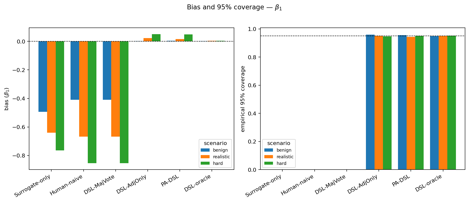
3 shows that Surrogate-only, Human-naive, and DSL-MajVote are all substantially biased, with bias ranging from \(-0.41\) in the benign scenario to \(-0.85\) in the hard scenario and empirical \(95\%\) coverage equal to \(0.000\) in every cell. Standard DSL does not repair this failure when its “gold” audit label is itself noisy: the correction removes surrogate-side bias relative to the audit label, and therefore inherits bias in that label. Majority vote also fails because coder errors are correlated through shared item difficulty, so the bias common to both coders survives aggregation.
5.0.0.2 Claim 2: audit-corrected estimators recover validity.
3 also shows that DSL-AdjOnly, PA-DSL, and the infeasible DSL-oracle all sit within Monte Carlo error of zero bias and report empirical coverage in \([0.94, 0.96]\) across all three scenarios. Adjudication-only DSL is design-valid because it uses only the adjudicated subset \(\{R_i V_i = 1\}\) with the joint sampling weight \(1/(\pi \rho_i).\) The price it pays is that the unadjudicated coder labels \(G_{i,1}, G_{i,2}\) on the rest of the audit set are simply discarded.
5.0.0.3 Claim 3: PA-DSL improves efficiency where the inner layer has signal.
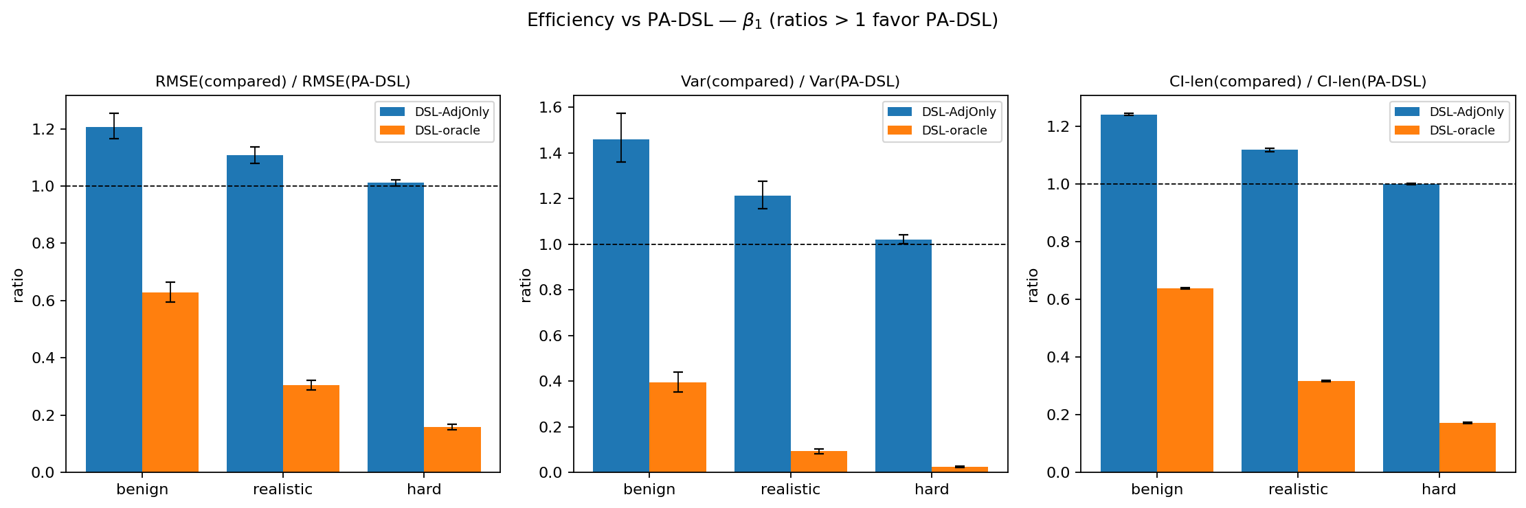
4 reports the efficiency ratios of PA-DSL versus DSL-AdjOnly (the strongest feasible baseline) and DSL-oracle (the infeasible benchmark), with paired-bootstrap \(95\%\) CIs over the \(1{,}000\) Monte Carlo replications. Relative to DSL-AdjOnly, the RMSE ratio is \(1.21\) (\(95\%\) CI \([1.17, 1.25]\)) in benign, \(1.11\) (\([1.08, 1.14]\)) in realistic, and \(1.01\) (\([1.00, 1.02]\)) in hard, with corresponding variance ratios \(1.46\) (\([1.36, 1.57]\)), \(1.21\) (\([1.16, 1.27]\)), and \(1.02\) (\([1.00, 1.04]\)). The benign and realistic gains are clear; the hard-regime ratio’s lower bound sits within \(5 \times 10^{-4}\) of \(1\), so \(\mathrm{\small PA-DSL}{}\) reverts to the adjudication-only benchmark when the inner layer has no recoverable signal. In this scenario, the surrogate is weak, the coders are noisy, and the adjudication budget is sparse, so predicting \(A_i\) from \((Q_i,X_i,G_{i,1},G_{i,2})\) buys little leverage beyond the \(\pi_i\rho_i\)-weighted adjudicated subset. The reversion is the right behavior: PA-DSL does not manufacture signal absent from the inner features. Classification-oriented diagnostics in Appendix 18 show the same pattern at the prediction level: \(\widehat\mu(Z_i)\) improves on \(\widehat g(B_i)\) in the benign and realistic settings, but adds little signal in the hard setting.
5.0.0.4 Claim 4: Detox replicates the qualitative pattern.
2 shows the same comparison on the Wikipedia Detox corpus with the Dawid–Skene proxy truth (\(\beta_1 = -1.42\) on logged_in). The plug-in baselines and the standard-DSL
variants fed with noisy gold are biased by \(0.33\)–\(0.39\) with zero empirical coverage; DSL-AdjOnly and PA-DSL both achieve
near-zero bias and coverage at or slightly above \(95\%\). PA-DSL’s RMSE ratio against DSL-AdjOnly is \(1.18\) (\(95\%\) paired-bootstrap CI \([1.10, 1.27]\)) and its CI-length ratio is \(1.13\) (\([1.12, 1.13]\)); both are clearly above
\(1\), so the efficiency gain is statistically distinguishable from the no-gain point. The same qualitative ranking is reproduced under the hard-majority and soft-mean proxies in 13.
As above, this is evidence for the sampling-and-adjudication machinery under real text and real crowdworker disagreement, with respect to the constructed proxy truth rather than an observed latent construct.
| Method | Bias | MC SD | RMSE | Coverage | CI len. |
|---|---|---|---|---|---|
| Surrogate-only | \(\phantom{-}0.387\) | \(0.000\) | \(0.387\) | \(0.000\) | \(0.043\) |
| Human-naive | \(\phantom{-}0.332\) | \(0.045\) | \(0.335\) | \(0.000\) | \(0.208\) |
| DSL-MajVote | \(\phantom{-}0.334\) | \(0.037\) | \(0.336\) | \(0.000\) | \(0.179\) |
| DSL-AdjOnly | \(\phantom{-}0.005\) | \(0.098\) | \(0.098\) | \(0.935\) | \(0.368\) |
| \(\phantom{-}0.009\) | \(\best{0.082}\) | \(\best{0.083}\) | \(0.975\) | \(\best{0.327}\) | |
| DSL-oracle | \(\phantom{-}0.005\) | \(0.035\) | \(0.036\) | \(0.965\) | \(0.144\) |
6 Discussion↩︎
PA-DSL extends design-based supervised learning to hierarchical annotation pipelines in which adjudication is treated as the gold-standard label but is available only for a subset of audited cases. The results suggest several practical lessons for designing and analyzing such pipelines.
6.0.0.1 When the proposal helps and when it does not.
PA-DSL delivers efficiency gains over adjudication-only DSL when the audit-tier features \(Z_i=(Q_i,X_i,G_{i,1},G_{i,2})\) predict the adjudicated label \(A_i\) beyond the outer features \(B_i=(Q_i,X_i)\). When this inner layer contains little additional signal, PA-DSL behaves like the adjudication-only benchmark, as in the hard synthetic regime. This pattern is formalized by the variance comparison in 8.0.0.10, where the gain over adjudication-only DSL is proportional to the \(Z\)-explainable component \(\mu_0(Z_i)-g_0(B_i)\). The inner ablations in 15 also show that the augmented-IPW form is not merely cosmetic: regression-only correction produced severe undercoverage in the realistic and hard regimes, underscoring the need to combine the outcome model with the known adjudication design.
6.0.0.2 Design implications.
The design sensitivity analysis in 14 suggests a practical operating range in the settings we studied: audit rates of roughly \(\pi \in [0.10,0.20]\) combined with disagreement-driven adjudication at \(\bar\rho \in [0.10,0.25]\). Disagreement-driven adjudication should include a positive adjudication floor even among agreement cases; otherwise, the design cannot identify error patterns in apparently easy items. More generally, the two-coder setup used in our experiments is not required by the framework: \(Z_i\) may include any audit-tier information observed when \(R_i=1\), including \(K_i\) coder labels, coder identities, agreement indicators, vote shares, uncertainty scores, or other metadata. The same inner correction applies as long as the adjudication probability \(\rho_i=P(V_i=1\mid R_i=1,Z_i)\) is known and bounded away from zero. The realized audit and adjudication probabilities should also be recorded with the labels, since PA-DSL relies on known \(\pi_i\) and \(\rho_i\) rather than estimating them after the fact. A pilot audit can help assess whether coder labels contain enough signal about the adjudicated construct to justify collecting additional human labels before increasing the adjudication budget.
6.0.0.3 Scope and limitations.
Although LLM-based annotation is one motivating use case, PA-DSL is a classifier-agnostic design-based correction: the surrogate \(Q_i\) may come from an LLM, a supervised classifier, a rules-based score, or any other automated labeling system observed on the full frame. However, PA-DSL is intended for prospective, known-probability audit/adjudication designs, or for settings in which the audit and adjudication probabilities can be reconstructed from the design record. It is not a generic post hoc correction for arbitrary deterministic review pipelines: if audited or adjudicated cases were selected using undocumented rules, or if some design strata have zero adjudication probability, the required positivity and ignorability conditions may fail.
Validity also relies on 3. We interpret this assumption as requiring adjudication to recover the target label under the adjudication protocol. 17 shows that PA-DSL inherits adjudicator bias relative to \(Y^{\star}_i\) when 3 fails. Thus, PA-DSL corrects the sampling and measurement structure only relative to the adjudicated construct; it cannot by itself guarantee that the adjudication protocol captures the substantive construct researchers intended. Estimators that remain valid under imperfect adjudication, treating \(A_i\) as a noisy proxy with a known design weight, are a natural next step.
The Detox study should be interpreted in this same spirit. It is a semi-synthetic evaluation using real text and real crowdworker disagreement, but the audit/adjudication indicators are re-drawn with known probabilities and the target is a held-out reference-panel operationalization rather than an external field-validated oracle. Non-binary outcomes, scores nonlinear in \(Y^{\star}_i\), and dependent-class missingness lie outside the current scope.
7 Prevalence as a Special Case↩︎
The population prevalence \(\psi = \mathbb{E}[Y^{\star}]\) is the special case of the outcome-affine framework in which the score is \(Y^{\star}_i - \psi\). The PA-DSL estimator instantiates as \(\hat{\psi} = N^{-1} \sum_i \widetilde{Y}_i\) with \(\widetilde{Y}_i\) from 4 , and the empirical-variance standard error \(\widehat{\mathrm{SE}}(\hat{\psi}) = (N(N-1))^{-1/2} \bigl(\sum_i (\widetilde{Y}_i - \hat{\psi})^2\bigr)^{1/2}\) is consistent for \(N^{-1/2}\) times the standard deviation of the influence function in 6 . 3 reports the synthetic results for this target across the three scenarios; the qualitative ranking matches the \(\beta_1\) results in the main text.
| Scenario | Method | Bias | MC SD | RMSE | Coverage | CI len. |
|---|---|---|---|---|---|---|
| benign | Surrogate-only | \(\phantom{-}0.0905\) | \(0.0012\) | \(0.0905\) | \(0.000\) | \(0.0047\) |
| Human-naive | \(\phantom{-}0.0010\) | \(0.0110\) | \(0.0111\) | \(0.898\) | \(0.0354\) | |
| DSL-MajVote | \(\phantom{-}0.0008\) | \(0.0085\) | \(0.0086\) | \(0.817\) | \(0.0232\) | |
| DSL-AdjOnly | \(\phantom{-}0.0003\) | \(0.0078\) | \(0.0078\) | \(0.945\) | \(0.0305\) | |
| \(\phantom{-}0.0003\) | \(\best{0.0063}\) | \(\best{0.0063}\) | \(0.949\) | \(\best{0.0247}\) | ||
| DSL-oracle | \(-0.0000\) | \(0.0042\) | \(0.0042\) | \(0.948\) | \(0.0163\) | |
| realistic | Surrogate-only | \(-0.0605\) | \(0.0012\) | \(0.0605\) | \(0.000\) | \(0.0049\) |
| Human-naive | \(\phantom{-}0.0014\) | \(0.0173\) | \(0.0174\) | \(0.692\) | \(0.0354\) | |
| DSL-MajVote | \(\phantom{-}0.0011\) | \(0.0162\) | \(0.0162\) | \(0.570\) | \(0.0266\) | |
| DSL-AdjOnly | \(-0.0002\) | \(0.0193\) | \(0.0193\) | \(0.941\) | \(0.0750\) | |
| \(-0.0003\) | \(\best{0.0170}\) | \(\best{0.0170}\) | \(0.951\) | \(\best{0.0669}\) | ||
| DSL-oracle | \(-0.0000\) | \(0.0056\) | \(0.0056\) | \(0.949\) | \(0.0220\) | |
| hard | Surrogate-only | \(-0.1434\) | \(0.0013\) | \(0.1435\) | \(0.000\) | \(0.0051\) |
| Human-naive | \(\phantom{-}0.0074\) | \(0.0223\) | \(0.0235\) | \(0.543\) | \(0.0357\) | |
| DSL-MajVote | \(\phantom{-}0.0074\) | \(0.0219\) | \(0.0231\) | \(0.434\) | \(0.0272\) | |
| DSL-AdjOnly | \(-0.0004\) | \(0.0341\) | \(0.0341\) | \(0.938\) | \(0.1294\) | |
| \(-0.0003\) | \(\best{0.0339}\) | \(\best{0.0338}\) | \(0.938\) | \(\best{0.1293}\) | ||
| DSL-oracle | \(\phantom{-}0.0000\) | \(0.0060\) | \(0.0060\) | \(0.948\) | \(0.0237\) |
8 Identification, Influence Function, and Variance↩︎
8.0.0.1 Notation and population nuisances.
For notational simplicity, this appendix writes the audit and adjudication probabilities as \(\pi(B_i)\) and \(\rho(Z_i)\). If the actual audit probability depends on additional observed design variables, those variables are either included in \(B_i\) or added to the conditioning set below. Likewise, any observed variables used to set adjudication probabilities are included in \(Z_i\). The arguments require only that the relevant conditional inclusion probabilities are known by design and bounded away from zero.
We write the population nuisance functions as \[\mu_0(z)=\mathbb{E}(A_i\mid Z_i=z,R_i=1,V_i=1), \qquad g_0(b)=\mathbb{E}\{\mu_0(Z_i)\mid B_i=b,R_i=1\}.\] Under Assumptions 1–3, \(\mu_0(Z_i)=\mathbb{E}(Y_i^\star\mid Z_i,R_i=1)\) and \(g_0(B_i)=\mathbb{E}(Y_i^\star\mid B_i)\). Thus \(g_0\) is a population target; it does not depend on the realized nuisance estimate or on a particular cross-fit pseudo-label.
8.0.0.2 Pointwise identification.
Under 1, \(\mathbb{E}[Y^{\star}_i \mid \boldsymbol{X}_i, Q_i] = \mathbb{E}[Y^{\star}_i \mid \boldsymbol{X}_i, Q_i, R_i = 1]\). Under 2 3, \(\mathbb{E}[Y^{\star}_i \mid Z_i, R_i = 1] = \mathbb{E}[A_i \mid Z_i, R_i V_i = 1] = \mu_0(Z_i)\). Composing, \(\mathbb{E}[\mu_0(Z_i) \mid B_i, R_i = 1] = \mathbb{E}[Y^{\star}_i \mid B_i, R_i = 1] = \mathbb{E}[Y^{\star}_i \mid B_i] = g_0(B_i)\).
8.0.0.3 Design-validity of \(\tilde{Y}_i\).
Fix arbitrary nuisance functions \(\eta=(\mu,g)\). For audited units define \[M_i(\mu)=\mu(Z_i)+\frac{V_i}{\rho(Z_i)}\{A_i-\mu(Z_i)\}.\] When the nuisances are estimated by cross-fitting, the following argument is understood conditionally on the training folds, so that \(\mu\) and \(g\) are fixed functions for the evaluation fold.
First consider the inner correction. Conditional on \(R_i=1\) and \(Z_i\), \[\begin{align} E\{M_i(\mu)\mid R_i=1,Z_i\} &= \mu(Z_i)+ E\left[ \frac{V_i}{\rho(Z_i)}\{A_i-\mu(Z_i)\} \mid R_i=1,Z_i \right] \\ &= \mu(Z_i)+ E\{A_i-\mu(Z_i)\mid R_i=1,Z_i,V_i=1\} \\ &= E(A_i\mid R_i=1,Z_i,V_i=1). \end{align}\] By adjudication correctness, \(A_i=Y_i^\star\) on \(\{R_iV_i=1\}\), and by adjudication ignorability, \[E(A_i\mid R_i=1,Z_i,V_i=1) = E(Y_i^\star\mid R_i=1,Z_i).\] Hence \[E\{M_i(\mu)\mid R_i=1,Z_i\} = E(Y_i^\star\mid R_i=1,Z_i).\]
No restriction on the joint distribution of \((G_{i,1},G_{i,2})\) is used here: once we condition on \(Z_i\), the coder labels are simply observed covariates, and all coder dependence or bias is part of the conditional mean \(\mu_0(Z_i)\).
Now consider the outer correction. Conditional on \(B_i\), \[\begin{align} E\{\tilde{Y}_i(\eta)\mid B_i\} &= g(B_i)+ E\left[ \frac{R_i}{\pi(B_i)} \{M_i(\mu)-g(B_i)\} \mid B_i \right] \\ &= g(B_i)+ E\{M_i(\mu)-g(B_i)\mid R_i=1,B_i\} \\ &= E\{M_i(\mu)\mid R_i=1,B_i\}. \end{align}\] Using iterated expectations and the inner result, \[\begin{align} E\{M_i(\mu)\mid R_i=1,B_i\} &= E\left[ E\{M_i(\mu)\mid R_i=1,Z_i\} \mid R_i=1,B_i \right] \\ &= E\left[ E(Y_i^\star\mid R_i=1,Z_i) \mid R_i=1,B_i \right] \\ &= E(Y_i^\star\mid R_i=1,B_i). \end{align}\] Finally, by audit ignorability, \[E(Y_i^\star\mid R_i=1,B_i)=E(Y_i^\star\mid B_i).\] Therefore \[E\{\tilde{Y}_i(\eta)\mid B_i\} = E(Y_i^\star\mid B_i).\] Since \(X_i\) is measurable with respect to \(B_i\), \[E\left[ X_i\{\tilde{Y}_i(\eta)-\operatorname{expit}(X_i^\top\beta)\} \right] = E\left[ X_i\{Y_i^\star-\operatorname{expit}(X_i^\top\beta)\} \right].\] At \(\beta=\beta_0\), the right-hand side is zero by definition of \(\beta_0\). Thus \(E\{m(W_i;\beta_0,\eta)\}=0\) for every fixed nuisance pair \(\eta\). This fixed-nuisance statement establishes design-unbiasedness of the score, but it does not imply that arbitrary inconsistent nuisance estimators have the same first-order expansion. The influence-function representation below is obtained by expanding around \(\eta_0=(\mu_0,g_0)\) and therefore requires the stated cross-fit nuisance convergence conditions.
8.0.0.4 Influence function.
The cross-fit estimator \(\hat{\psi}\) admits the asymptotic linear expansion \(\sqrt N (\hat{\psi} - \psi) = N^{-1/2} \sum_i \varphi(W_i; \mu_0, g_0) + o_p(1)\) with influence function \[\varphi(W_i; \mu_0, g_0) = g_0(B_i) - \psi + \frac{R_i}{\pi_i}\bigl[\mu_0(Z_i) - g_0(B_i)\bigr] + \frac{R_i V_i}{\pi_i \rho_i}\bigl[A_i - \mu_0(Z_i)\bigr]. \label{eq:if}\tag{6}\] The estimator \(\hat{\beta}\) from 5 has influence function \[\mathbf{H}^{-1}\,\boldsymbol{X}_i\,\bigl(\widetilde{Y}_i(\eta_0) - \operatorname{expit}(\boldsymbol{X}_i^\top \beta_0)\bigr), \qquad \mathbf{H} = \mathbb{E}[\boldsymbol{X}_i \boldsymbol{X}_i^\top\,\operatorname{expit}'(\boldsymbol{X}_i^\top \beta_0)],\] obtained directly from the M-estimator score \(m(W_i; \beta_0, \eta_0)\); the prevalence-target \(\varphi\) is not the right object for \(\hat{\beta}\) because the logistic score is not the prevalence influence function.
8.0.0.5 Why no product-rate condition is required.
Let \(\delta_g(B) = \hat{g}(B) - g_0(B)\) and \(\delta_\mu(Z) = \hat{\mu}(Z) - \mu_0(Z)\). Direct expansion of \(\widetilde{Y}_i\) gives \[\widetilde{Y}_i(\hat{\eta}) - \widetilde{Y}_i(\eta_0) = \Bigl(1 - \frac{R_i}{\pi_i}\Bigr)\delta_g(B_i) + \frac{R_i}{\pi_i} \Bigl(1 - \frac{V_i}{\rho_i}\Bigr)\delta_\mu(Z_i), \label{eq:nuis-perturb}\tag{7}\] so that \(m(W_i;\beta_0,\hat{\eta}) - m(W_i;\beta_0,\eta_0) = \boldsymbol{X}_i \cdot [\text{r.h.s.\;of \ref{eq:nuis-perturb}}]\). The two nuisance errors enter linearly, but each is multiplied by a known-design, conditionally mean-zero sampling residual. This is why the argument requires only \(L^2\) consistency of the nuisance estimators, rather than a product-rate condition.
8.0.0.6 Leakage-free nested cross-fitting.
We first analyze a leakage-free nested version of the estimator. For a held-out evaluation fold \(\mathcal{F}_k\), the inner nuisance used to construct audit pseudo-labels for the outer training sample is fit without using observations from \(\mathcal{F}_k\). The outer nuisance used to evaluate \(\mathcal{F}_k\) is therefore trained on pseudo-labels that contain no information from the held-out fold. Conditional on the training data for that fold, the nuisance functions are fixed with respect to the evaluation observations.
For such an evaluation observation, the conditional means of both bracketed factors in 7 are zero: \[\mathbb{E}\!\left[1 - \frac{R_i}{\pi_i} \,\middle|\, B_i\right] = 0\] by 1, and \[\mathbb{E}\!\left[ \frac{R_i}{\pi_i} \Bigl(1 - \frac{V_i}{\rho_i}\Bigr) \,\middle|\, Z_i,B_i \right] = 0\] by 2; the inner factor has conditional mean zero given \(R_i=1\) and \(Z_i\). Hence \[\mathbb{E}\!\Bigl[ m(W_i;\beta_0,\hat{\eta}) - m(W_i;\beta_0,\eta_0) \,\Big|\, \text{training data} \Bigr] = \mathbf{0}. \label{eq:cond-zero-rem}\tag{8}\] Thus the nuisance error contributes only a centered empirical-process remainder.
Because \(\pi_i\) and \(\rho_i\) are bounded away from zero, and \(\mathbb{E}\|\boldsymbol{X}_i\|^{2+\delta}<\infty\), there is a finite constant \(C\) such that \[\mathbb{E}\!\Bigl[ \bigl\| m(W_i;\beta_0,\hat{\eta}) - m(W_i;\beta_0,\eta_0) \bigr\|^2 \,\Big|\, \text{training data} \Bigr] \leq C\left( \|\hat{g}-g_0\|_{2,X,B}^2 + \|\hat{\mu}-\mu_0\|_{2,X,Z}^2 \right), \label{eq:l2-rem-bound}\tag{9}\] where \[\|h\|_{2,X,B}^2 = \mathbb{E}\!\left[\|\boldsymbol{X}_i\|^2 h(B_i)^2\right], \qquad \|r\|_{2,X,Z}^2 = \mathbb{E}\!\left[\|\boldsymbol{X}_i\|^2 r(Z_i)^2\right].\] Therefore, \[\sqrt N(P_N-P) \{m(W;\beta_0,\hat{\eta})-m(W;\beta_0,\eta_0)\} = O_p\!\left( \|\hat{g}-g_0\|_{2,X,B} + \|\hat{\mu}-\mu_0\|_{2,X,Z} \right) = o_p(1),\] under cross-fit \(X\)-weighted \(L^2\)-consistent nuisance estimation.
Combining this centered empirical-process bound with the fixed-nuisance design-unbiasedness result above and a standard mean-value expansion in \(\beta\) around \(\beta_0\) gives the asymptotic linear expansion in 1 for the leakage-free nested estimator. No product-rate condition appears because the known design weights make the linear nuisance remainder conditionally mean-zero.
8.0.0.7 Shared-partition cross-fitting.
Algorithm 2 uses a computationally simpler shared-partition implementation, in which the same folds are used in the inner and outer passes. For fold \(\mathcal{F}_k\), write \(\hat{g}_{\mathrm{sp}}^{(-k)}\) for the outer nuisance actually used by the algorithm. Let \(\hat{g}_{\mathrm{lf}}^{(-k)}\) denote the leakage-free counterpart: the outer nuisance that would be obtained by constructing each training pseudo-label \(\widehat M_j\), \(j\notin\mathcal{F}_k\), using an inner fit that excludes both \(\mathcal{F}_k\) and \(\mathcal{F}_{\mathrm{fold}(j)}\).
The shared-partition estimator has the same first-order expansion as the leakage-free estimator provided the leakage remainder satisfies \[\frac{1}{\sqrt N}\sum_{k=1}^{K}\sum_{i \in \mathcal{F}_k} X_i\Bigl(1 - \frac{R_i}{\pi_i}\Bigr) \bigl\{ \hat{g}_{\mathrm{sp}}^{(-k)}(B_i) - \hat{g}_{\mathrm{lf}}^{(-k)}(B_i) \bigr\} = o_p(1). \label{eq:sp}\tag{10}\] To see this, add and subtract the leakage-free score: \[\begin{align} &\frac{1}{\sqrt N} \sum_{k=1}^{K} \sum_{i \in \mathcal{F}_k} \left[ m\bigl(W_i;\beta_0,\hat{\mu}^{(-k)},\hat{g}_{\mathrm{sp}}^{(-k)}\bigr) - m(W_i;\beta_0,\eta_0) \right] \notag\\ &\quad= \frac{1}{\sqrt N} \sum_{k=1}^{K} \sum_{i \in \mathcal{F}_k} \left[ m\bigl(W_i;\beta_0,\hat{\mu}^{(-k)},\hat{g}_{\mathrm{lf}}^{(-k)}\bigr) - m(W_i;\beta_0,\eta_0) \right] \notag\\ &\qquad+ \frac{1}{\sqrt N}\sum_{k=1}^{K}\sum_{i \in \mathcal{F}_k} X_i\Bigl(1 - \frac{R_i}{\pi_i}\Bigr) \bigl\{ \hat{g}_{\mathrm{sp}}^{(-k)}(B_i) - \hat{g}_{\mathrm{lf}}^{(-k)}(B_i) \bigr\}. \label{eq:sp-decomp} \end{align}\tag{11}\] The first term is \(o_p(1)\) by the leakage-free argument. The second term is \(o_p(1)\) by condition 10 . Hence the shared-partition estimator has the same asymptotic linear representation as the leakage-free estimator whenever condition 10 holds.
8.0.0.8 Discussion of the shared-partition stability condition.
Condition 10 is a stability condition on the indirect leakage created by reusing the same fold partition in the inner and outer stages. It is expected to hold when the inner learner is stable under adding or removing one fold, the outer learner is Lipschitz-stable in its training responses, and the resulting difference \[\|\hat{g}_{\mathrm{sp}}^{(-k)}-\hat{g}_{\mathrm{lf}}^{(-k)}\|_{2,X} = o_p(1)\] is sufficiently small that the weighted empirical average in 10 is \(o_p(1)\). This is plausible for stable nuisance learners in fixed-dimensional smooth classes, such as the fixed-hyperparameter \(L^2\)-regularized logistic regressions used in the experiments, under standard nonsingularity and bounded-moment conditions. A formal verification requires learner-specific deletion stability controlling the effect of excluding \(\mathcal{F}_k\) from the inner fits on the resulting outer nuisance. The condition may fail for highly adaptive nuisance procedures, including tuning, stacking, or model selection performed inside the cross-fitting loop, because such procedures can transmit evaluation-fold information into \(\hat{g}_{\mathrm{sp}}^{(-k)}\).
8.0.0.9 Variance decomposition.
Let \[H(Z, B) \;=\; \mu_0(Z) - g_0(B), \qquad \varepsilon \;=\; A - \mu_0(Z),\] so that \(\varphi(W; \mu_0, g_0) = \bigl(g_0(B) - \psi\bigr) + \tfrac{R}{\pi(B)} H(Z,B) + \tfrac{R V}{\pi(B)\,\rho(Z)} \varepsilon\). Because \(\mathbb{E}[H(Z, B) \mid B, R = 1] = 0\) (by definition of \(g_0\)) and \(\mathbb{E}[\varepsilon \mid Z, R = 1, V = 1] = 0\) (by definition of \(\mu_0\)), the three summands are mutually orthogonal martingale increments. Iterated expectations give \(\mathbb{E}[(R/\pi(B))^2 H(Z,B)^2] = \mathbb{E}[H(Z,B)^2 / \pi(B)]\) and \(\mathbb{E}[(R V/(\pi(B)\rho(Z)))^2 \varepsilon^2] = \mathbb{E}[\sigma_A^2(Z) / (\pi(B)\,\rho(Z))]\) where \(\sigma_A^2(Z) = \mathrm{Var}(A \mid Z, R = 1, V = 1)\), so \[\mathrm{Var}[\varphi] \;=\; \mathrm{Var}[g_0(B)] \;+\; \mathbb{E}\!\left[\frac{H(Z, B)^2}{\pi(B)}\right] \;+\; \mathbb{E}\!\left[\frac{\sigma_A^2(Z)}{\pi(B)\,\rho(Z)}\right]. \label{eq:var-ng}\tag{12}\] For constant \(\pi(B) \equiv \pi\) and \(\rho(Z) \equiv \rho\), \(\mathrm{Var}[\varphi] = \mathrm{Var}[g_0(B)] + \pi^{-1} \mathbb{E}[(\mu_0(Z) - g_0(B))^2] + (\pi \rho)^{-1} \mathbb{E}[\sigma_A^2(Z)]\). At \(\pi = \rho = 1\) this collapses to \(\mathrm{Var}(A)\) via the law of total variance, as it must.
8.0.0.10 Efficiency gain over DSL-AdjOnly.
The adjudication-only DSL pseudo-outcome treats \(R_i V_i\) as the sampling indicator and uses the joint design weight \(1/(\pi(B_i)\,\rho(Z_i))\) to debias the outer regression \(\hat{g}\), giving influence function \(\varphi_{\mathrm{adj}} = (g_0(B) - \psi) + (R V/(\pi(B)\,\rho(Z)))(A - g_0(B))\) — structurally a single-stage AIPW with the joint sampling indicator. Decomposing \(A - g_0(B) = H(Z, B) + \varepsilon\) and applying the same orthogonality argument, \[\mathrm{Var}[\varphi_{\mathrm{adj}}] \;=\; \mathrm{Var}[g_0(B)] \;+\; \mathbb{E}\!\left[\frac{H(Z, B)^2}{\pi(B)\,\rho(Z)}\right] \;+\; \mathbb{E}\!\left[\frac{\sigma_A^2(Z)}{\pi(B)\,\rho(Z)}\right]. \label{eq:var-adj}\tag{13}\] Subtracting 12 from 13 gives \[\mathrm{Var}[\varphi_{\mathrm{adj}}] - \mathrm{Var}[\varphi] \;=\; \mathbb{E}\!\left[ \frac{1 - \rho(Z)}{\pi(B)\,\rho(Z)}\, \bigl(\mu_0(Z) - g_0(B)\bigr)^2 \right] \;\geq\; 0, \label{eq:var-gain}\tag{14}\] which simplifies to \(((1-\rho)/(\pi\rho))\,\mathbb{E}[(\mu_0(Z) - g_0(B))^2]\) for constant \(\pi, \rho\).
For the logistic-regression target in the main text, the same comparison applies to the covariance of the score influence function \(X_i\{\widetilde{Y}_i(\eta_0)-\operatorname{expit}(X_i^\top\beta_0)\}\). In particular, the corresponding difference in score covariance matrices is \[\Omega_{\mathrm{adj}} - \Omega \;=\; \mathbb{E}\!\left[ X_i X_i^\top \frac{1 - \rho(Z_i)}{\pi(B_i)\,\rho(Z_i)}\, \bigl(\mu_0(Z_i) - g_0(B_i)\bigr)^2 \right], \label{eq:omega-gain}\tag{15}\] which is positive semidefinite. Applying the usual M-estimation transformation, the corresponding asymptotic covariance difference for \(\hat{\beta}\) is \[H^{-1}(\Omega_{\mathrm{adj}}-\Omega)H^{-1\top},\] also positive semidefinite. Thus the scalar comparison in 14 has the same interpretation for the main logistic-regression estimand: PA-DSL removes the extra \(\rho(Z_i)^{-1}\) inflation from the component of adjudicated truth explained by audit-tier features beyond \(B_i\).
The PA-DSL estimator does not reduce the residual adjudication noise term \(\sigma_A^2(Z)\), which can only be learned from adjudicated units and remains weighted by \(1/(\pi(B)\rho(Z))\) in both estimators. What PA-DSL does is move the \(Z\)-explainable component \(\mu_0(Z) - g_0(B)\) from the sparse adjudication weight \(1/(\pi(B)\rho(Z))\) to the larger audit weight \(1/\pi(B)\). The gain in 14 is therefore large precisely when (i) adjudication is sparse, so \(\rho(Z)\) is small, and (ii) the audit-level features \(Z\) explain substantial variation in the adjudicated label, and collapses to zero when \(Z\) has no incremental predictive power over \(B\).
9 Why build on DSL rather than PPI?↩︎
Prediction Powered Inference (PPI) is a closely related prediction-assisted inference framework [9]. We build on DSL because our measurement process is explicitly design-based: the audit and adjudication samples are drawn with known probabilities chosen by the analyst. The DSL pseudo-outcome is therefore the natural object to extend, and partial adjudication is handled by nesting a second known-weight correction inside the usual audit correction. This is not a claim that PPI is inappropriate; rather, deriving a partially adjudicated PPI analogue is a separate extension. Recent benchmarking finds that DSL can be competitive with, and often more efficient than, PPI for LLM-based parameter estimation, though performance varies by setting [26].
10 Implementation Details↩︎
All nuisances are L2-regularized logistic regression unless otherwise noted (\(C = 1\), max-iter \(2000\)); predictions are clipped to \([10^{-3}, 1 - 10^{-3}]\) to bound the importance weights in 4 . Cross-fitting uses \(K = 5\) folds, stratified on twenty \(Q\)-quintile \(\times\) \(B_{\mathrm{diff}}\)-quartile strata where \(B_{\mathrm{diff}} = 1 - 2|p^\star - 0.5|\) is the boundary statistic. \(\beta\) is fit by damped iteratively reweighted least squares with a \(10^{-6}\) ridge for numerical stability; standard errors use the empirical sandwich on the cross-fit pseudo-outcome.
The estimators evaluated in the main text and appendices are: Surrogate-only, Human-naive, DSL-MajVote (two coders, ties randomly broken), DSL-AdjOnly, DSL-oracle, PA-DSL (logistic, baseline inner features), PA-DSL-coder (logistic, coder-pair features), PA-DSL-IPW-only (inner \(\hat{\mu} \equiv 0\); pure Horvitz–Thompson at the inner stage), and PA-DSL-Reg-only (no \(V/\rho\) debias at the inner stage; pure regression).
11 Synthetic Data-Generating Process↩︎
Each replication generates \(N = 50{,}000\) units. Covariates \(\boldsymbol{X}_i\) comprise an intercept and \(p = 5\) continuous features drawn from a multivariate normal with unit variances and equicorrelation \(\rho_{\mathrm{cov}} = 0.2\). Latent labels are \(Y^{\star}_i \mid \boldsymbol{X}_i \sim \text{Bernoulli}(\operatorname{expit}(\boldsymbol{X}_i^\top \boldsymbol{\beta}))\), with \(\boldsymbol{\beta}= (-0.4,\, 1.0,\, -0.8,\, 0.6,\, 0.0,\, 0.0)^\top\). The boundary statistic is \(B_{i,\mathrm{diff}} = 1 - 2|\operatorname{expit}(\boldsymbol{X}_i^\top \boldsymbol{\beta}) - 0.5|\).
Three latent difficulty channels are \[\begin{align} D_i &= \delta_0 + \delta_1 B_{i,\mathrm{diff}} + \delta_2 |X_{i,1}| + \delta_3 |X_{i,2}| + U_i, \quad U_i \sim N(0, \sigma_D^2),\\ H_i &= \eta_1 X_{i,3} + \eta_2 X_{i,4} + \xi_i, \quad \xi_i \sim N(0, \sigma_H^2),\\ M_i &= \zeta_1 X_{i,4} + \zeta_2 X_{i,5} + \nu_i, \quad \nu_i \sim N(0, \sigma_M^2). \end{align}\] The surrogate is \(Q_i = \operatorname{expit}(\tau_0 + \tau_1 Y^{\star}_i + \tau_2 X_{i,1} + \tau_3 X_{i,2} - \lambda_D D_i - \lambda_M M_i + \varepsilon_i)\) with \(\varepsilon_i \sim N(0, \sigma_Q^2)\). Coder \(j\) has sensitivity intercept \(\alpha^{(1)}_j \sim N(a_{\text{sens}}, \sigma_{\text{coder}}^2)\) and specificity intercept \(\alpha^{(0)}_j \sim N(a_{\text{spec}}, \sigma_{\text{coder}}^2)\); conditional on \(Y^{\star}_i\) and the difficulty channels, \(\mathbb{P}(G_{ij} = 1 \mid Y^{\star}_i = 1) = \operatorname{expit}(\alpha^{(1)}_j - \gamma_D D_i - \gamma_H H_i)\) and the symmetric expression on \(Y^{\star}_i = 0\). The audit indicator is uniform Bernoulli(\(\pi\)); audited units draw two distinct coders without replacement. Under uniform adjudication \(\rho_i \equiv \bar\rho\); under disagreement-based adjudication \(\rho_i \propto d_0 + d_1 \mathbf{1}\{G_{i,1} \neq G_{i,2}\}\) rescaled to mean \(\bar\rho\).
| Parameter | Benign | Realistic | Hard |
|---|---|---|---|
| \(\tau_1\) | 2.0 | 1.5 | 1.0 |
| \(\lambda_D\) | 0.5 | 1.0 | 1.4 |
| \(\lambda_M\) | 0.4 | 0.8 | 1.2 |
| \(\sigma_Q\) | 0.7 | 1.0 | 1.4 |
| \(\sigma_{\text{coder}}\) | 0.20 | 0.35 | 0.50 |
| \(\gamma_D\) | 0.5 | 1.0 | 1.4 |
| \(\gamma_H\) | 0.35 | 0.7 | 1.0 |
| Adjudication policy | uniform | disagreement | disagreement |
| \(\bar\rho\) | 0.25 | 0.25 | 0.10 |
12 Inner-Stage Feature Ablation↩︎
5 ablates the inner nuisance feature set (\(R = 200\) replications). Coder-pair features add no detectable improvement over the baseline feature set in any scenario. We adopt the baseline-feature logistic variant as the default PA-DSL throughout the main text.
| Scenario | Inner stage | Bias | MC SD | RMSE | Coverage | CI len. |
|---|---|---|---|---|---|---|
| benign | DSL-AdjOnly (no inner) | \(0.006\) | \(0.057\) | \(0.057\) | \(0.965\) | \(0.213\) |
| (logistic, baseline) | \(0.005\) | \(\best{0.047}\) | \(\best{0.047}\) | \(0.950\) | \(\best{0.173}\) | |
| (logistic, +coder) | \(0.006\) | \(0.048\) | \(0.048\) | \(0.935\) | \(0.174\) | |
| realistic | DSL-AdjOnly (no inner) | \(0.027\) | \(0.130\) | \(0.133\) | \(0.960\) | \(0.524\) |
| (logistic, baseline) | \(0.015\) | \(\best{0.116}\) | \(\best{0.117}\) | \(0.945\) | \(\best{0.466}\) | |
| (logistic, +coder) | \(0.016\) | \(0.118\) | \(0.118\) | \(0.940\) | \(0.469\) | |
| hard | DSL-AdjOnly (no inner) | \(0.052\) | \(\best{0.248}\) | \(\best{0.253}\) | \(0.950\) | \(\best{0.932}\) |
| (logistic, baseline) | \(0.051\) | \(0.250\) | \(0.255\) | \(0.945\) | \(\best{0.932}\) | |
| (logistic, +coder) | \(0.052\) | \(0.251\) | \(0.255\) | \(0.950\) | \(0.948\) |
13 Detox: Additional Proxy Truths↩︎
6 reports the Detox \(\beta_1\) comparison under the two proxy-truth constructions not shown in the main text: hard majority vote on the reference panel (\(R = 50\) replications, target \(\beta_1 = -1.50\)) and the soft mean attack share (\(R = 50\), target \(\beta_1 = -1.10\)). The qualitative ranking is unchanged: the plug-in baselines and DSL-MajVote fed with noisy gold miss the proxy with zero coverage on the hard-majority proxy; DSL-AdjOnly and PA-DSL both achieve nominal coverage; PA-DSL reduces RMSE relative to DSL-AdjOnly by \(13\)–\(16\%\). Because \(Y^{\star}\) is unobservable in the field, the displayed truth is the proxy refit on the full reference panel; DSL-oracle is therefore an upper bound on achievable accuracy under each proxy, not an oracle for the latent attack construct.
| Proxy | Method | Bias | MC SD | RMSE | Coverage | CI len. |
|---|---|---|---|---|---|---|
| hard maj. | Surrogate-only | \(\phantom{-}0.393\) | \(0.000\) | \(0.393\) | \(0.00\) | \(0.050\) |
| Human-naive | \(\phantom{-}0.409\) | \(0.046\) | \(0.412\) | \(0.00\) | \(0.208\) | |
| DSL-MajVote | \(\phantom{-}0.416\) | \(0.039\) | \(0.418\) | \(0.00\) | \(0.180\) | |
| DSL-AdjOnly | \(-0.005\) | \(0.102\) | \(0.101\) | \(0.98\) | \(0.443\) | |
| \(-0.006\) | \(\best{0.088}\) | \(\best{0.087}\) | \(0.98\) | \(\best{0.398}\) | ||
| DSL-oracle | \(-0.000\) | \(0.047\) | \(0.046\) | \(0.96\) | \(0.179\) | |
| soft mean | Surrogate-only | \(\phantom{-}0.285\) | \(0.000\) | \(0.285\) | \(0.00\) | \(0.035\) |
| Human-naive | \(\phantom{-}0.009\) | \(0.046\) | \(0.046\) | \(0.98\) | \(0.208\) | |
| DSL-MajVote | \(\phantom{-}0.017\) | \(0.038\) | \(0.041\) | \(1.00\) | \(0.179\) | |
| DSL-AdjOnly | \(\phantom{-}0.013\) | \(0.067\) | \(0.068\) | \(0.90\) | \(0.259\) | |
| \(\phantom{-}0.012\) | \(\best{0.056}\) | \(\best{0.057}\) | \(0.98\) | \(\best{0.225}\) | ||
| DSL-oracle | \(\phantom{-}0.003\) | \(0.019\) | \(0.019\) | \(1.00\) | \(0.097\) |
14 Design Curves: Audit and Adjudication Sweep↩︎
The three benign / realistic / hard scenarios in the main text are static design points. To answer the practical question “how much adjudication should an analyst buy, and how should adjudicated items be selected?", we sweep the audit rate \(\pi \in \{0.05, 0.10, 0.20\}\), the mean adjudication rate \(\bar\rho \in \{0.10, 0.25, 0.50\}\), the adjudication policy \(\in \{\)uniform, disagreement\(\}\), and an optional positivity floor \(\rho_{\min,\text{agree}} \in \{0, 0.05\}\) on agreement cases (under disagreement-driven adjudication, units with \(G_{i,1} = G_{i,2}\) would otherwise receive \(\rho \approx d_0/(d_0 + d_1)\,\bar\rho\), which can be very small). Other parameters are fixed at the realistic-scenario values (4); each cell uses \(R = 200\) replications.
5 reports the \(\beta_1\) RMSE ratio \(\mathrm{RMSE}(\mathrm{\small DSL-AdjOnly}) / \mathrm{RMSE}(\mathrm{\small PA-DSL}{})\) across the sweep, with paired-bootstrap \(95\%\) CIs. Three patterns emerge. First, disagreement-driven adjudication is consistently higher in point estimate than uniform adjudication across the grid: the disagreement panels (bottom row) sit roughly \(5\)–\(10\) percentage points above the uniform panels at matched mean budget, with overlapping but offset CIs at \(R = 200\) replications per cell. The mechanism is that adjudication concentrates on the cases where coder labels disagree — exactly where the inner \(\hat{\mu}\) has the largest residual to debias and the most leverage to add over DSL-AdjOnly. Second, the gain is largest at the moderate audit rate \(\pi = 0.10\) under disagreement (orange line, peak ratio \(1.15\) at \(\bar\rho = 0.10\)); \(\pi = 0.05\) leaves too little inner training data, while \(\pi = 0.20\) already buys enough adjudicated truth that the inner correction has less to add and the ratio drops toward \(1.06\) at \(\bar\rho = 0.50\). Third, the positivity floor on agreement cases has only small, mostly within-CI effects on the realistic-scenario sweep. The \(\rho_{\min,\text{agree}} = 0.05\) panels are nearly indistinguishable from the no-floor panels. The floor would matter more at scenarios with very small \(d_0/(d_0 + d_1)\) ratios (where the unfloored agreement-case \(\rho_i\) is close to zero); we leave that exploration to future work. For practical pipelines, the sweep suggests targeting \(\pi \in [0.10, 0.20]\) with disagreement-driven adjudication at \(\bar\rho \in [0.10, 0.25]\) as a sweet spot of audit cost vs.inferential efficiency.

15 Inner-Stage AIPW Ablation↩︎
PA-DSL’s inner stage combines an outcome model \(\hat{\mu}(Z)\) with a Horvitz–Thompson correction \(V/\rho\) around it. We isolate the contribution of each piece by re-running the synthetic analysis with inner-stage variants:
IPW-only. Set \(\hat{\mu} \equiv 0\), so \(\widehat M_i = (V_i/\rho_i)\,A_i\). Pure Horvitz–Thompson at the inner stage. Design-valid (unbiased for any nuisance choice) but does not exploit the surrogate or coder labels at the inner stage, and is sensitive to small \(\rho_i\) values.
IPW-only (trunc). As IPW-only but with the truncated weight \(\rho_i \mapsto \max(\rho_i, 0.05)\), capping \(1/\rho_i \le 20\). This is a numerical sensitivity check that disentangles weight-stability failures from fundamental design issues; truncation breaks design-validity under the original sampling weights.
Reg-only. Skip the \(V/\rho\) debias; set \(\widehat M_i = \hat{\mu}(Z_i)\). Pure regression. Lower variance than IPW-only when \(\hat{\mu}\) fits well, but the sandwich SE no longer accounts for the nuisance estimation noise, so confidence intervals can severely undercover.
7 reports the comparison on the three synthetic scenarios at \(R = 200\).
The IPW-only variant pays a steep variance price for not exploiting the inner features. In benign and realistic, RMSE roughly triples; in hard the estimator becomes numerically unstable. The disagreement-weighted adjudication policy at \(\bar\rho = 0.10\) produces audited units with \(\rho_i\) as low as \(\sim\!0.02\) (\(1/\rho_i \approx 45\)), and the \(\widetilde{Y}_i\) pseudo-outcomes inherit those weights. Two of \(R = 200\) hard-scenario replications produce pseudo-outcome distributions extreme enough to push the logistic IRLS solver outside its convergence regime, yielding \(|\hat{\beta}_1|\) on the order of \(10^5\)–\(10^6\) and dominating the column means.1
The Reg-only variant achieves lower MC variance than full PA-DSL in benign and realistic, and looks nearly unbiased, but the empirical coverage drops to \(0.645\) in benign, \(0.260\) in realistic, and \(0.070\) in hard. The sandwich SE on \((\boldsymbol{X}_i, \widetilde{Y}_i)\) is computed as if \(\widehat M_i = \hat{\mu}(Z_i)\) were a fixed quantity, but \(\hat{\mu}\) is itself a noisy estimator; without the \(V/\rho\) correction term to absorb that noise into the estimating equation, the SE underestimates the true variability and CIs miss the truth far more often than nominal.
The full PA-DSL estimator avoids both failure modes: the regression component \(\hat{\mu}(Z)\) stabilizes the inner pseudo-label relative to IPW-only (cutting variance by an order of magnitude), while the \(V/\rho\) correction restores design validity and makes the sandwich variance reflect the adjudication-stage uncertainty.
| Scenario | Inner stage | Bias | MC SD | RMSE | Coverage | CI len. |
|---|---|---|---|---|---|---|
| benign | DSL-AdjOnly | \(\phantom{-}0.006\) | \(0.057\) | \(0.057\) | \(0.965\) | \(0.213\) |
| (full) | \(\phantom{-}0.005\) | \(\best{0.047}\) | \(\best{0.047}\) | \(0.950\) | \(\best{0.173}\) | |
| (IPW-only) | \(\phantom{-}0.020\) | \(0.139\) | \(0.140\) | \(0.970\) | \(0.559\) | |
| (IPW-only, trunc)\(^\dagger\) | \(\phantom{-}0.020\) | \(0.139\) | \(0.140\) | \(0.970\) | \(0.559\) | |
| (Reg-only) | \(\phantom{-}0.001\) | \(0.046\) | \(0.046\) | \(0.645\) | \(0.079\) | |
| DSL-oracle | \(\phantom{-}0.006\) | \(0.029\) | \(0.030\) | \(0.935\) | \(0.110\) | |
| realistic | DSL-AdjOnly | \(\phantom{-}0.027\) | \(0.130\) | \(0.133\) | \(0.960\) | \(0.524\) |
| (full) | \(\phantom{-}0.015\) | \(\best{0.116}\) | \(\best{0.117}\) | \(0.945\) | \(\best{0.466}\) | |
| (IPW-only) | \(\phantom{-}0.085\) | \(0.285\) | \(0.296\) | \(0.970\) | \(1.115\) | |
| (IPW-only, trunc)\(^\dagger\) | \(\phantom{-}0.085\) | \(0.285\) | \(0.296\) | \(0.970\) | \(1.115\) | |
| (Reg-only) | \(-0.007\) | \(0.066\) | \(0.066\) | \(0.260\) | \(0.053\) | |
| DSL-oracle | \(\phantom{-}0.009\) | \(0.039\) | \(0.040\) | \(0.925\) | \(0.148\) | |
| hard | DSL-AdjOnly | \(\phantom{-}0.052\) | \(\best{0.248}\) | \(\best{0.253}\) | \(0.950\) | \(\best{0.932}\) |
| (full) | \(\phantom{-}0.051\) | \(0.250\) | \(0.255\) | \(0.945\) | \(\best{0.932}\) | |
| (IPW-only) | numerically unstable; see footnote in prose | |||||
| (IPW-only, trunc) | \(-0.258\) | \(0.176\) | \(0.312\) | \(0.655\) | \(0.695\) | |
| (Reg-only) | \(-0.014\) | \(0.123\) | \(0.123\) | \(0.070\) | \(0.023\) | |
| DSL-oracle | \(\phantom{-}0.010\) | \(0.042\) | \(0.043\) | \(0.945\) | \(0.158\) | |
16 Shared-Partition vs.\(K^2\)-fold Cross-fit↩︎
1(b) covers two implementations: leakage-free nested cross-fitting and the shared-partition 2 under stability condition 10 . 8 reports a paired sanity check on the realistic scenario (\(N=50{,}000\), \(\bar\rho=0.25\), disagreement-weighted adjudication, \(R=200\) replications, paired per-rep seeds): the two implementations give the same point estimate to within Monte Carlo error, consistent with 10 holding for the fixed-hyperparameter L2-regularized logistic nuisances used here.
| Cross-fit scheme | Bias | MC SD | RMSE | Coverage | CI len. | Mean abs.diff. |
|---|---|---|---|---|---|---|
| Shared partition ([alg:ngdsl]) | \(0.0148\) | \(0.1160\) | \(0.1166\) | \(0.945\) | \(0.4664\) | — |
| \(K^2\)-fold double cross-fit | \(0.0148\) | \(0.1159\) | \(0.1165\) | \(0.945\) | \(0.4666\) | \(0.0009\) |
The mean absolute paired difference \(0.0009\) is two orders of magnitude smaller than either implementation’s MC SD (\(\approx 0.116\)), and the sample correlation between the two paired estimates is \(0.99995\). The shared-partition shortcut reproduces the leakage-free estimator essentially exactly at the cost of \(K - 1\) fewer inner fits per outer fold.
17 Imperfect-Adjudication Sensitivity↩︎
3 (\(A_i = Y^{\star}_i\) on adjudicated units) is load-bearing for design-validity with respect to \(Y^{\star}_i\). To illustrate what happens when adjudication is systematically wrong, 9 compares the realistic scenario (\(N=50{,}000\), \(R=500\) replications) under correct adjudication against a biased-adjudication mechanism that flips \(A_i\) with probability \(0.075\) when \(X_{i,1} > 0\) and \(0.025\) otherwise — a 5% average error correlated with the regression’s primary covariate.
Under correct adjudication, both DSL-AdjOnly and PA-DSL are unbiased and have nominal coverage. Under biased adjudication, both inherit the adjudicator bias relative to \(Y^{\star}_i\) and miss the truth at higher rates. PA-DSL retains its design-validity for the adjudicated construct (the function \(\mathbb{E}[A_i \mid \boldsymbol{X}_i]\)), but that construct is no longer \(\mathbb{E}[Y^{\star}_i \mid \boldsymbol{X}_i]\) when adjudicators systematically disagree with the latent label. The audit/adjudication design probabilities cannot recover information adjudicators do not provide; designs that further relax 3 require an additional measurement tier (e.g. treating \(A_i\) as a noisy proxy of \(Y^{\star}_i\) with a known design weight).
| Adjudication target | Method | Bias | MC SD | RMSE | Coverage | CI len. |
|---|---|---|---|---|---|---|
| Correct \(A = \Ystar\) | DSL-AdjOnly | \(\phantom{-}0.020\) | \(0.135\) | \(0.136\) | \(0.952\) | \(0.522\) |
| \(\phantom{-}0.013\) | \(\best{0.123}\) | \(\best{0.123}\) | \(0.940\) | \(\best{0.467}\) | ||
| DSL-oracle | \(\phantom{-}0.007\) | \(0.037\) | \(0.038\) | \(0.946\) | \(0.148\) | |
| Biased \(A\) | DSL-AdjOnly | \(-0.124\) | \(0.131\) | \(0.180\) | \(0.790\) | \(0.508\) |
| \(-0.129\) | \(\best{0.122}\) | \(\best{0.178}\) | \(0.784\) | \(\best{0.472}\) | ||
| DSL-oracle | \(\phantom{-}0.007\) | \(0.037\) | \(0.038\) | \(0.946\) | \(0.148\) |
18 Classification-oriented predictor diagnostics.↩︎
Although PA-DSL targets downstream estimating equations rather than individual classification, we report supplemental prediction diagnostics to help interpret the efficiency mechanism. Table 10 compares the full-frame surrogate \(Q_i\), the outer nuisance prediction \(\widehat g(B_i)\), and the inner nuisance prediction \(\widehat\mu(Z_i)\), evaluated against the adjudicated/proxy target. The final AIPW pseudo-outcomes are not included as classifiers because they are estimating-equation devices and need not be calibrated probabilities or lie in \([0,1]\).
The diagnostics support the mechanism described in Appendix 8. In the benign and realistic synthetic settings, \(\widehat\mu(Z_i)\) improves prediction relative to \(\widehat g(B_i)\), indicating that the audit-tier features add adjudication-relevant information beyond \(B_i=(Q_i,X_i)\). In the hard setting, this incremental signal is small and the inner prediction does not improve on \(\widehat g(B_i)\), matching the near-zero efficiency gain reported in the main results. The Detox study shows a modest but consistent improvement from \(\widehat\mu(Z_i)\), consistent with the observed PA-DSL efficiency gain.
| \(Q_i\) | \(\widehat g(B_i)\) | \(\widehat\mu(Z_i)\) | |||||
|---|---|---|---|---|---|---|---|
| 2-3(lr)4-5(lr)6-7 Study / scenario | AUC | Brier | AUC | Brier | AUC | Brier | RMS\((\widehat\mu-\widehat g)\) |
| Synthetic: benign | 0.949 | 0.118 | 0.968 | 0.070 | 0.990 | 0.037 | 0.300 |
| Synthetic: realistic | 0.776 | 0.206 | 0.864 | 0.150 | 0.869 | 0.146 | 0.156 |
| Synthetic: hard | 0.639 | 0.292 | 0.810 | 0.176 | 0.794 | 0.182 | 0.064 |
| Detox | 0.903 | 0.096 | 0.902 | 0.095 | 0.908 | 0.088 | 0.096 |
References↩︎
The truncated variant PA-DSL-IPW-only-trunc caps \(1/\rho_i \le 20\) and restores numerical stability on the hard scenario at the cost of a small bias relative to the original design. We report it as a sensitivity check that disentangles a small-\(\rho\) stability artefact from a fundamental design defect; under the original (un-truncated) sampling weights, IPW-only is the design-valid pure-Horvitz–Thompson baseline.↩︎