Mutable Low-Rank Sketches for Retrain-Free Recommendation
July 16, 2026
Abstract
A common bottleneck in two-stage recommendation is embedding staleness: when a user rates a new item, their embedding remains fixed until the next retrain cycle. We propose mutable sketches, which store each user’s preferences in a KP-tree (a sparse segment tree with sum aggregation), fit a low-rank projection once, and recompute embeddings on-the-fly as ratings arrive. We prove that each new observation monotonically tightens the prediction error envelope (Theorem [thm:monotone]), a guarantee that FunkSVD and eALS lack. On KuaiRec, the mutable sketch achieves 0.810 RMSE at 1.8% data read vs.ALS 0.822 at 100%, with 8\(\times\) faster per-batch updates. A new user receives personalized recommendations in \(<\)1 ms after their first rating, with no model retraining required. A comparison of sampling strategies across density regimes shows that the KP-tree’s norm-proportional sampling provides 40–130% better item coverage on sparse data (\(<\)1% density), while uniform sampling suffices on dense matrices.
1 Introduction↩︎
In two-stage recommendation [1], [2], user embeddings typically cannot update until the model retrains — hours for neural methods, minutes for ALS [3]. Even incremental methods such as eALS [4] and FunkSVD [3] modify the factorization directly, coupling data freshness to model recomputation.
In production feature stores, this decomposition is standard: user features are updated continuously while the model remains fixed [5]. We apply the same principle to collaborative filtering: each user’s preference vector lives in a KP-tree [6], [7] — structurally a sparse segment tree with sum aggregation — and embeddings are recomputed by projecting through a fixed low-rank basis fitted once from a sublinear sketch. When a user rates a new item, a logarithmic-time tree insert changes the stored preference vector, and the user’s embedding is recomputed by projecting through the fixed basis — no gradient computation, no model parameters touched. Each insert also keeps the sampling distribution consistent by propagating through internal sums, so the sketch can be rebuilt from the current state at any time without reconstructing auxiliary structures — a property that dense segment trees share but Fenwick trees and hash-map-based alternatives do not support with logarithmic-time weighted sampling.
Prior KP-tree work [7]–[10] used the structure for static sketch construction only; we exploit its mutation capability. Our contributions are:
Mutable sketches: user-side embedding updates in \(O(\log n)\) per rating with no gradient computation — retrain-free between drift-triggered refits (§2.1, §4).
Monotonic improvement: a proof that each new observation tightens the projected-error envelope (Theorem 1), a guarantee FunkSVD and eALS lack (§2.2).
Consistent sampling under mutation: the sampling distribution remains valid after every insert, enabling immediate sketch patches and near-free drift signals (§2.3, §4).
Evaluation across density regimes: six datasets spanning six orders of magnitude in density, locating the crossover (\(\sim\)5%) below which norm-proportional sampling beats uniform (§3).
Randomized matrix sketching [11], [12] produces static low-rank approximations; streaming extensions [13] handle sliding windows but cannot incorporate arbitrary updates without full rebuilds. Sarwar et al. [14] and Brand [15] update the thin SVD via rank-one perturbation with periodic re-orthogonalization to control numerical drift; eALS [4] uses element-wise factor updates per rating. All three modify the factorization itself, coupling data freshness to model recomputation. Streaming recommenders such as RMFX [16] use pairwise BPR [17] over a fixed-size reservoir with SGD updates; dynamic-embedding methods (AutoEmb [18], DESS [19]) optimize embedding dimension allocation rather than update latency. All of these approaches pay gradient or solver cost per update, whether on explicit ratings or implicit feedback [20]. Our approach is orthogonal: hold the model fixed and update only the data structure, eliminating gradient computation on the user side entirely.
A parallel line of systems work accelerates freshness at other layers of the serving stack. Ekko [21] disseminates trained model updates across geo-distributed inference clusters in seconds via peer-to-peer synchronization; LiveUpdate [22] refreshes embedding tables on idle inference-node CPUs, exploiting the low-rank structure of embedding-table gradients (LoRA-style) to reach minute-scale freshness with negligible serving impact. Both accelerate model freshness — how quickly new parameters reach serving. We target the layer upstream of both: data freshness, where a new rating changes the served embedding with no parameters trained or shipped at all. The distinction from LiveUpdate is instructive: both exploit low-rank structure, but LiveUpdate uses it to compress gradient updates, while we use it to project fresh data through a fixed basis — no gradients anywhere in the update path. The three layers compose rather than compete.
2 Mutable Sketches via KP-Trees↩︎
The key idea is to decouple data freshness from model freshness. We store each user’s preference vector in a data structure that supports efficient sampling and point updates, fit a low-rank projection \(V_k\) once from a small sketch, and recompute user embeddings on-the-fly by projecting through the fixed \(V_k\) whenever the data changes. The projection never degrades as observations accumulate (Theorem 1).
2.1 Sketch Construction and Serving↩︎
Definition 1 (KP-Tree). Given \(\mathbf{a} \in \mathbb{R}^n\), the KP-tree is a binary tree of depth \(\lceil \log_2 n \rceil\) where leaf \(j\) stores \(|a_j|\) and each internal node stores the sum of its children. It supports Sample (draw \(j \propto |a_j|\)), Query (look up \(a_j\)), and Update (modify \(a_j\) and propagate sums) — all in \(O(\log n)\).
To build the sketch, sample \(r\) rows (users) proportional to row norms; for each, sample \(c\) columns proportional to entry magnitudes. Extract values at the union of sampled columns to form an \(r \times |\mathcal{C}|\) sketch \(S\), then fit truncated SVD: \(S \approx U_k \Sigma_k V_k^T\), producing item embeddings (rows of \(V_k\)). Total cost: \(O(m + rc \log n)\) where \(m\) is the number of users (rows), independent of the number of non-zero entries (\(\text{nnz}\)) in the rating matrix.
At serving time, for user \(i\), read their preference values over the sketch’s column set from the KP-tree, center, and project: \(\mathbf{u}_i = (\mathbf{a}_i - \bar{\mathbf{c}}) V_k \in \mathbb{R}^k\). This embedding is used for ANN retrieval (e.g., FAISS [23]) or direct prediction via \(\hat{a}_{ij} = \mathbf{u}_i V_k^T + \bar{c}_j\), where \(\bar{c}_j\) is the per-item mean rating over the sketch columns, correcting for item popularity bias. When user \(i\) rates item \(j\), insert \(a_{ij}\) into their KP-tree in \(O(\log n)\). The next query reads the updated tree, producing a better projection through the same \(V_k\) — no model parameters change.
2.2 Monotonic Improvement Guarantee↩︎
Theorem 1 (Shrinking projected-error envelope). Let \(V_k\) be a fixed orthonormal basis, \(P = V_k V_k^T\), and \(\mathbf{a}^*\) a user’s true preference vector. Let \(\mathbf{a}^{(t)}\) be the observed version at time \(t\) (unobserved entries zero). If \(\mathbf{a}^{(t+1)}\) sets one unobserved entry \(j\) to its true value \(a^*_j\), then: \[\| P\mathbf{a}^{(t+1)} - P\mathbf{a}^* \| \;\leq\; \sqrt{\|\mathbf{a}^{(t)} - \mathbf{a}^*\|^2 - (a^*_j)^2} \;<\; \|\mathbf{a}^{(t)} - \mathbf{a}^*\|.\]
Proof. Let \(\mathbf{e}^{(t)} = \mathbf{a}^{(t)} - \mathbf{a}^*\) denote the error at time \(t\). Since entry \(j\) is unobserved at time \(t\), we have \(e^{(t)}_j = -a^*_j\). At time \(t{+}1\), entry \(j\) is set to \(a^*_j\), so \(e^{(t+1)}_j = 0\) and \(e^{(t+1)}_i = e^{(t)}_i\) for \(i \neq j\). That is, \(\mathbf{e}^{(t+1)}\) equals \(\mathbf{e}^{(t)}\) with component \(j\) zeroed out, giving \(\|\mathbf{e}^{(t+1)}\|^2 = \|\mathbf{e}^{(t)}\|^2 - (a^*_j)^2\). Since \(P = V_k V_k^T\) is an orthogonal projection, \(\|P\mathbf{x}\| \leq \|\mathbf{x}\|\) for all \(\mathbf{x}\). Applying this to \(\mathbf{x} = \mathbf{e}^{(t+1)}\) yields the result. (Note: we assume the observed rating equals the true preference. With zero-mean observation noise of variance \(\sigma^2\), the squared bound holds in expectation with an additive \(\sigma^2\) term: \(\mathbb{E}\|P\mathbf{e}^{(t+1)}\|^2 \leq \|\mathbf{e}^{(t)}\|^2 - (a^*_j)^2 + \sigma^2\), which is monotone whenever the signal exceeds the noise variance.) ◻
The common incremental baselines lack this property. FunkSVD offers no monotonicity guarantee (SGD on new batches can overwrite base-data signal), eALS stagnates without item-factor updates, and Brand’s rank-one perturbation [15] accumulates numerical drift over many updates. The mutable sketch sidesteps these failure modes because it does not modify the factorization — only the data changes.
2.3 Consistent Sampling Under Mutation↩︎
Any key-value store can serve the projection step — reading a user’s preferences and multiplying by \(V_k\) — following the feature-store pattern common in production systems [5]. The KP-tree’s contribution is to the sketch construction step, where \(V_k\) is built or rebuilt by sampling rows proportional to norms and columns proportional to entry magnitudes (Section 2.1). A key-value store would require scanning all users to compute norms and maintaining per-user alias tables for weighted column sampling, both at cost proportional to the total number of ratings and both invalidated by each new insert. The KP-tree avoids this by providing norm-proportional sampling in \(O(\log n)\) with consistency maintained after each update. As we show experimentally (Section 3.4), this advantage is density-dependent: norm-proportional sampling outperforms uniform sampling below \(\sim\)5% density, a regime that covers many production workloads. On denser data, uniform sampling suffices and the KP-tree’s sampling capability offers no benefit, though its \(O(\log n)\) point queries remain useful for embedding computation.
3 Experimental Evaluation↩︎
We evaluate primarily on KuaiRec [24] (4.7M interactions, 1.4K users, 3.3K items, 99.6% dense — a fully-observed dataset), with four sparse benchmarks: Amazon Electronics 2023 [25] (5M ratings, 3.3M users, 672K items, 0.0002% dense), Amazon Video Games 2023 [25] (4.6M ratings, 2.8M users, 137K items, 0.001% dense), Amazon Music 2023 [25] (128K ratings, 101K users, 71K items, 0.002% dense), and Book-Crossing [26] (247K ratings, 3.7K users, 186K items, 0.048% dense). All experiments use rank \(k{=}10\), sketch size \(200{\times}100\). We report RMSE on a held-out test set throughout: static experiments use an 80/20 random split; streaming experiments train on 60% of the data and stream the remaining 40% in equal-sized batches. Most experiments run on a single-core laptop; ML-25M [27] and Goodreads Comics [28] experiments run on a 32-vCPU ARM server with 256 GB RAM. Table 1 summarizes asymptotic costs.
| Method | Fit / Retrain | Online update |
|---|---|---|
| ALS | \(O(T \cdot \text{nnz} \cdot k)\) | Full refit |
| eALS | \(O(T \cdot \text{nnz} \cdot k)\) | \(O(k^2 \cdot |R_u|)\)/user |
| FunkSVD | \(O(T \cdot \text{nnz} \cdot k)\) | \(O(b \cdot k \cdot T)\) |
| Ours | \(O(m + rc \log n)\) | \(O(b \log n)\) |
3.1 Static Accuracy↩︎
We first ask how the sketch compares to full-data baselines when all ratings are available at training time. On KuaiRec (Table 2), the mutable sketch achieves 0.810 RMSE while reading 1.8% of the matrix, compared to 0.822 for ALS at 100%. On sparser benchmarks the gap widens: Amazon Music (0.002% dense) yields 1.029 RMSE, competitive with mean baselines while reading \(<\)1% of a matrix too large for full SVD. Amazon Video Games (0.001% dense) yields 1.562 RMSE with norm-proportional sampling. In these regimes most full-data methods either exceed memory (Full SVD) or overfit (ALS achieves 4.62 on Amazon Music). On ML-1M (4.2% dense), the gap is larger (Table 3), reflecting sparser sampling coverage. Increasing the sketch size from \(200{\times}100\) (2% data) to \(800{\times}200\) (10.8%) narrows the gap from 0.113 to 0.085, illustrating the accuracy-data tradeoff at moderate density.
| Method | RMSE |
|---|---|
| Full SVD | 0.8037 |
| ALS [3] | 0.8216 |
| eALS [4] | 0.8240 |
| FunkSVD [3] | 0.8037 |
| Item Mean | 0.8556 |
| Mutable sketch + bias (ours, 1.8% data) | 0.8099 |
| Method | RMSE | Data |
|---|---|---|
| ALS [3] | 0.863 | 100% |
| Ours (\(800{\times}200\)) | 0.948 | 10.8% |
| Ours (\(200{\times}100\)) | 0.976 | 2.0% |
| Item Mean | 0.979 | 100% |
3.2 Online Updates↩︎
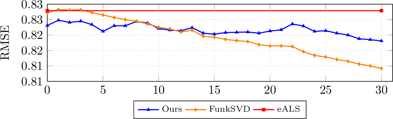
Static accuracy matters less if the model cannot incorporate new ratings without a full retrain. We hold out 40% of the training ratings and stream them in 30 equal-sized batches (\({\sim}\)50K ratings each on KuaiRec), measuring test RMSE after each batch (Table 4, Figure 1). All methods start from the same 60% base data and receive identical streaming input.
| Ours | FunkSVD | eALS | |
|---|---|---|---|
| Final RMSE | 0.818\(\downarrow\) | 0.809\(\downarrow\) | 0.828\(\downarrow\) |
| Avg batch | 90ms | 200ms | 730ms |
| Monotonic? | Yes | No | No |
| Obs.-to-serve | 2.5ms | 200ms | 730ms |
The sketch’s RMSE improves from 0.823 to 0.818 over 30 batches (Figure 1), consistent with Theorem 1. FunkSVD starts slightly worse (0.827) but converges steadily, crossing the sketch around batch 12 and reaching 0.809 by batch 30. eALS converges from 0.828 at batch 0 to 0.828 at batch 30 after re-solving affected user factors with each batch. Per-batch latency is 90 ms for the sketch vs. ms for FunkSVD and 730 ms for eALS. End-to-end observation-to-serve latency is 2.5 ms P95.
3.3 Cold-Start Latency↩︎
A key operational concern is how quickly a brand-new user receives personalized recommendations. With the mutable sketch, a new user’s KP-tree can be created, their ratings inserted, and their embedding computed via the existing \(V_k\) in a single serving call — no model retrain required (Table 5, Figure 2).
| Ratings | P50 (ms) | P95 (ms) | RMSE |
|---|---|---|---|
| 1 | 0.49 | 1.36 | 0.873 |
| 3 | 0.66 | 2.48 | 0.874 |
| 10 | 0.75 | 2.48 | 0.865 |
| 50 | 5.06 | 9.75 | 0.863 |
| eALS per-user solve: \(\sim\)5 ms. ALS requires full retrain (\(\sim\)36 s). | |||
With a single rating, the sketch serves a personalized recommendation in 0.49 ms P50, and RMSE (0.873) is within 0.06 of full-data ALS (0.822) — the projection through \(V_k\) leverages the latent structure learned from all other users. Latency scales with rating count but remains sub-10 ms even at 50 ratings.

3.4 Sampling Strategy and Density↩︎
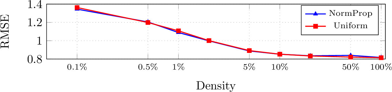
The KP-tree’s norm-proportional sampling maintains \(O(\log n)\) consistency under mutation. We compare it against uniform random sampling across density regimes (Table 6). On sparse data, norm-proportional sampling concentrates on signal-carrying rows, yielding 40–130% more sketch columns (e.g., 591 vs. on Amazon Music). On dense data, uniform coverage is already representative. Bias correction (subtracting per-item means \(\bar{c}_j\)) helps on moderately sparse datasets like Goodreads Comics (0.930\(\to\)0.844) and Amazon Music (1.087\(\to\)1.060), but can hurt on extremely sparse data where the column means are poorly estimated.
| Dataset | Density | NormProp | +Bias | Uniform | +Bias |
|---|---|---|---|---|---|
| Amazon Electronics | 0.0002% | 1.407 | 1.498 | 1.680 | 1.709 |
| Amazon Video Games | 0.001% | 1.485 | 1.562 | 1.729 | 1.747 |
| Amazon Music | 0.002% | 1.087 | 1.060 | 1.152 | 1.354 |
| Goodreads Comics | 0.018% | 0.930 | 0.844 | 1.049 | 0.984 |
| ML-25M | 0.048% | 0.944 | 0.897 | 0.999 | 0.955 |
| KuaiRec | 99.6% | 0.821 | 0.818 | 0.819 | 0.815 |
A density sweep on KuaiRec subsamples (Figure 3) places the crossover at roughly 5–10% density: norm-proportional sampling helps below this; the methods converge at 10–20%; uniform wins above 50%. Since many production systems operate well below 1% density, the KP-tree’s ability to maintain a consistent sampling distribution under mutation has practical value beyond its theoretical motivation.
4 Discussion↩︎
The mutable sketch has clear limitations. Accuracy depends on the sketch covering enough items; the approach works well when the item space is compact relative to the sketch size (KuaiRec: 3.3K items, 99% coverage) but degrades on large catalogs (Amazon Video Games: 137K items, \(<\)1% coverage). The fixed \(V_k\) accumulates staleness as the data distribution shifts, but the rate is density-dependent. On ultra-sparse data (Amazon Music, \(\sim\)1.3 ratings/user), \(V_k\) never goes stale: the sketch holds at 1.05 RMSE over 30 streaming batches while ALS degrades from 1.50 to 1.93 — periodic refit is indistinguishable from no refit because ALS cannot learn a better low-rank space from so few observations. On denser data (ML-1M), accuracy without refit plateaus \(\sim\)0.08 RMSE above periodic refit after 30 batches; refitting every 10 batches closes the gap at \(\sim\)13 s per refit. A hybrid strategy — continuous tree updates (milliseconds) with periodic SVD refit (seconds) — captures most of ALS’s accuracy on dense datasets and exceeds it on sparse ones. To trigger refits only when warranted, the KP-tree exposes two signals at negligible cost: norm divergence — total variation between the current and snapshot sampling distributions, \(O(1)\) per tree root — and projection residuals — \(\|\mathbf{a}_i - V_k V_k^T \mathbf{a}_i\| / \|\mathbf{a}_i\|\), the fraction of user signal outside \(V_k\). A three-tier controller monitors these: (1) tree-only updates when both signals are small, (2) a warm sketch patch — extract fresh values from updated trees for stale sketch rows, then re-run SVD on the patched sketch, skipping the distributed sampling phase — when residuals grow, or (3) a full \(V_k\) rebuild when norm divergence is large. On both Amazon Music and ML-1M, the controller stays on Tier 1 throughout (norm divergence reaches only 0.012–0.035), achieving 2.7–5.4\(\times\) speedup over periodic ALS by correctly avoiding unnecessary refits; multi-backend implementation details are in [29]. The formulation is pure collaborative filtering; non-ID features enter via the downstream ranker. Jointly encoding side features in the sketch is future work.
We validated serving latency on ML-10M (72K users, 10K items) using a ConcurrentHashMap-backed serving prototype on a single core (Table 8). KP-tree memory scales as \(O(r_i \log n)\) per user with \(r_i\) ratings; at 100M users with 50 ratings each, this totals \(\sim\)1 TB partitioned across cluster nodes, reducible via tiered storage since user trees are independent.
A related body of systems-ML work observes that tree-based sampling structures, while asymptotically optimal, are poorly suited to GPU workloads: tree traversals require pointer chasing across non-contiguous memory, and concurrent updates to shared internal nodes create thread contention that destroys parallelism. The prevailing alternative is to use Walker’s Alias Method [30] (\(O(1)\) sampling from a flat table), accept intentionally stale sampling probabilities for a fixed number of steps, and periodically rebuild the table using dense tensor operations. Our consistency experiment (Table 7) quantifies the cost of this staleness assumption: on Amazon Music (0.002% dense), sampling from stale distributions after streaming updates degrades RMSE by 0.32; on KuaiRec (99.6% dense), the cost is zero. This suggests that the alias-table approach is appropriate for dense or GPU-oriented workloads, while the KP-tree’s consistent sampling is more valuable for sparse, CPU-based serving — the regime we target. Our serving measurements (Table 8) are single-core CPU; we do not claim GPU compatibility. The same regime distinction applies to inference-side update systems: LiveUpdate [22] targets dense DLRM embedding tables of tens of terabytes on GPU inference clusters with terabytes of RAM per node, where LoRA gradient steps on idle CPUs are cheap relative to the serving fleet. We target the opposite corner — sparse rating matrices served from a single CPU core, where even one gradient step per update would dominate the sub-millisecond budget. These are different production niches, and the two mechanisms could compose: a mutable sketch for the sparse long tail alongside a LiveUpdate-style pipeline for the dense head.
The mutable sketch targets a different point in the latency-accuracy tradeoff than neural embeddings: sub-millisecond cold-start and monotonic safety, at the cost of initial accuracy below full-data methods on sparse matrices. It is weakest when maximum accuracy is required, when non-ID features are needed at retrieval, or when the pipeline is GPU-oriented. The low rank (\(k{=}10\)) of the sketch embedding is itself an advantage for retrieval: it avoids the curse of dimensionality that degrades tree-based and exact nearest-neighbor indices beyond \({\sim}20\) dimensions, and keeps ANN index sizes small.
| Dataset | Fresh | Stale | Gap |
|---|---|---|---|
| Amazon Music (0.002%) | 0.914 | 1.234 | 0.320 |
| KuaiRec (99.6%) | 0.818 | 0.818 | 0.000 |
5 Conclusion↩︎
We presented mutable sketches for recommendation that is retrain-free between drift-triggered refits: user-side updates never touch the model, and the model is refit only when cheap drift signals warrant it. The KP-tree’s ability to maintain a consistent sampling distribution under mutation enables instant embedding updates, immediate sketch patches, and a monotonic improvement guarantee. On KuaiRec, the sketch achieves competitive accuracy at 1.8% data read with 8\(\times\) faster updates than eALS; a new user gets personalized recommendations in \(<\)1 ms. The sampling advantage is density-dependent: valuable on sparse data typical of production systems, and unnecessary on dense research benchmarks. Code, datasets, and experiment scripts are available upon request.
| Component | P95 |
|---|---|
| User embedding computation | 2.45 ms |
| FAISS retrieval (top-10, Flat index) | 0.020 ms |
| End-to-end | \(\sim\)2.5 ms |
| P50: 0.71 ms. Mean: 1.08 ms. Throughput: 927 QPS. | |