Divergent Gaze Patterns in Artistic Viewing:
Spatial and Temporal Signatures of Attention Across
Autistic Individuals, Artists, and Neurotypical Observers
July 16, 2026
Abstract
How different populations visually explore artworks bears on cognitive science and on accessibility design, yet most eye-tracking work in autism has used social scenes rather than art, and has analysed where the eyes land while ignoring when and in what order. We present a comparative free-viewing study across three groups, autistic adults (ASD), trained artists, and neurotypical observers, who each viewed 30 paintings for 15 s. We introduce a directed, metric-grounded framework that compares groups along two complementary axes: a spatial axis, in which one group’s fixation-density map predicts another’s fixations under six saliency metrics (AUC-Judd, NSS, CC, SIM, KL, Information Gain); and a temporal axis, in which individual scanpaths are compared with MultiMatch, ScanMatch, a foveal-disc IoU score (FDISS), and dynamic time warping (DTW). Fixations are extracted uniformly for all groups with a dispersion-threshold algorithm. Three results converge. (i) Artists and neurotypicals are almost indistinguishable in both space (density-map correlation \(\text{CC}=0.96\)) and time (they form the most alignable scanpath pair), whereas ASD gaze diverges from both. (ii) ASD attention is dissociated: it matches artists’ wide spatial exploration (dispersion, explored area) but carries a distinct temporal signature, shorter fixations, less dwell, and the most idiosyncratic (least self-consistent) scanpaths of any group. (iii) ASD gaze is not selectively artist-like on any metric; if anything it is marginally closer to neurotypical. Together these findings indicate that autistic viewing of art is a distinct, group-specific attentional profile in both space and time, and they motivate population-conditioned models of aesthetic attention. We release all analysis code and per-stimulus results.
1 Introduction↩︎
Paintings are among the richest naturalistic stimuli for studying overt visual attention. Unlike sparse laboratory displays, an artwork combines low-level salience, recognisable objects and faces, and deliberate compositional structure, so that where a viewer chooses to look reflects the interplay of bottom-up conspicuity, semantic interest, and higher-level viewing strategy [1], [2]. Free-viewing of artworks therefore offers a natural setting in which to ask how perceptual expertise, prior experience, and cognitive style reshape the distribution, and the dynamics, of gaze.
Two populations are classic “non-normative” viewers. Artists, trained to attend to structural and compositional relationships rather than to isolated objects, distribute gaze more evenly and rely less on the semantically obvious [2], [3]. Autistic individuals (ASD) show atypical attention to faces and social cues [4]–[6], heightened engagement with local low-level features, and reduced influence of global semantic context; these tendencies are consistent with the weak-central-coherence account [7] and the enhanced-perceptual-functioning model [8], and free-viewing gaze in ASD is more strongly tied to pixel-level salience than to object- and semantic-level content [9]. Yet almost all of this evidence comes from social scenes and faces; how autistic observers deploy attention during aesthetic viewing of artworks is comparatively unexplored.
This leaves a deceptively simple question. Both artists and autistic observers attend to detail rather than to the single obvious focal point. Does ASD gaze during artwork viewing therefore resemble the detail-oriented gaze of trained artists, the gaze of neurotypical observers, or neither? A preliminary late-breaking study [1] suggested a dissociation at the level of spatial density maps, but it was limited in three ways that this paper addresses: it analysed only spatial density (discarding the temporal order of fixations), it relied on a single map per group per stimulus, and it was statistically underpowered.
We make four contributions. (1) A two-axis, directed, metric-grounded framework for cross-group gaze comparison that treats group-to-group similarity both as a saliency-prediction problem (spatial axis) and as a scanpath-comparison problem (temporal axis), using a uniform fixation-extraction pipeline applied identically to every group. (2) A three-group free-viewing comparison (artists, neurotypical observers, autistic adults) over 30 paintings, with fixations re-extracted from the raw signal, yielding \(2{,}091\) scanpaths and \(95{,}282\) fixations. (3) Evidence of a spatial–temporal dissociation in ASD: autistic gaze matches artists’ wide spatial exploration but has a distinct temporal signature, and is the most idiosyncratic (least self-consistent) of the three groups. (4) A clear ordering: artists and neurotypicals converge in both space and time, while ASD is not selectively artist-like on any of ten metrics.
2 Related Work↩︎
2.0.0.1 Expertise and gaze in art perception.
A substantial literature establishes that formal training reshapes how art is viewed. [2] found that artists distribute gaze more evenly across a composition and rely less on the salient objects that dominate novice viewing, and [3] report converging eye-movement correlates of visual-arts expertise. Because gaze on artworks is driven by compositional and stylistic structure that differs from everyday scenes, predicting it computationally is itself a domain-specific problem, addressed through domain adaptation [10], self-supervised learning [11], and dedicated art-viewing datasets [12]. We build on this line but ask a comparative, population-level question rather than modelling a single population.
2.0.0.2 Visual attention in autism.
Atypical gaze is among the most robust behavioural markers associated with ASD. Early scanning studies showed autistic individuals fixate faces and social scenes differently from neurotypical viewers [4], and eye-movement measures have been used as implicit indices of face processing [5], [6]. Two influential accounts predict a bias away from global, semantically driven looking: weak central coherence [7] and enhanced perceptual functioning [8]. Directly relevant, [9] used model-based eye tracking to show that free-viewing gaze in ASD is atypically driven by low-level pixel salience. Prior work concentrated on social and naturalistic scenes; free-viewing of paintings, where composition and aesthetics matter, remains largely unaddressed.
2.0.0.3 Comparing gaze: distributions and scanpaths.
For distribution-level comparison we build on the saliency-evaluation literature: [13] provide a systematic account of what location-based (AUC, NSS) and distribution-based (CC, SIM, KL) metrics measure, and [14] introduce an information-theoretic formulation (Information Gain). Although designed to score models, these metrics apply to any pair of fixation distributions: treating one group’s density map as the “model” and another group’s fixations as the “ground truth” yields a principled directional measure of cross-group similarity. The order and timing of fixations, however, are discarded by density maps. Scanpath-comparison measures recover them: MultiMatch decomposes similarity into shape, direction, length, position and duration [15]; ScanMatch adapts sequence alignment to binned fixation strings [16]; perceptually grounded overlap can be quantified with foveal discs [17]; and semantic similarity can be computed with vision–language models [18]. We combine both families into a single directed framework and, crucially, apply it to human populations rather than algorithms.
3 Data & Participants↩︎
Eye-tracking data were recorded with an SMI RED500 remote eye tracker at 500 Hz while participants freely viewed 30 colour paintings. Each stimulus was presented at \(1650\times1050\) px for \(\approx\)15 s (verified from the per-trial export timings), with no explicit task, so that recorded gaze reflects spontaneous exploration. The 30 paintings span landscapes, still lifes, portraits and abstract compositions. Each participant saw all 30 paintings, split across two blocks with no repetition, giving one scanpath per participant per painting. Three groups were recruited:
Artists (\(n=24\)): trained visual artists with \(\geq\)10 years of professional or semi-professional experience.
Neurotypical (\(n=32\)): no formal art training and no neurological diagnosis.
ASD (\(n=15\)): autistic adults diagnosed per ICD-11 [19] without co-occurring intellectual disability.
After quality control (Sec. 4.1), the analysis set comprises \(2{,}091\) scanpaths and \(95{,}282\) fixations (Art 712, Typ 940, ASD 439 scanpaths).
4 Methodology↩︎
We compare groups along two axes. The spatial axis (Sec. 4.2) asks how well one group’s fixation distribution predicts another’s. The temporal axis (Sec. 4.3) asks how similar the ordered fixation sequences are. Both consume a single set of fixations extracted uniformly for every group.
4.1 Fixation extraction↩︎
The averaged binocular point of regard was median-smoothed (15-sample window, \(\approx\)30 ms) to suppress remote-tracker jitter, then classified into fixations with the dispersion-threshold identification algorithm
(IDT) [20] as implemented in the eyefeatures library [21] (maximum dispersion \(\approx\)90 px \(\approx2^\circ\), minimum duration 100 ms). We deliberately did not use the
tracker’s own per-sample event labels, which on this recording are implausible (\(\sim\)47% of samples labelled saccade); a single dispersion rule applied to all groups avoids confounding group differences with
per-participant classifier behaviour. Scanpaths with fewer than four fixations were discarded. The procedure recovers physiological fixations (mean duration \(\approx\)200 ms, \(\approx\)46
fixations per 15 s viewing).
4.2 Spatial axis: density-map prediction↩︎
For each group \(g\) and stimulus \(s\) we pool the fixations of all participants in \(g\) and rasterise them, on a down-scaled \(210\times131\) grid, into a binary map \(Q^s_g\); smoothing with a 2-D Gaussian (\(\sigma\!\approx\!1^\circ\)) and normalising yields a continuous density map \(P^s_g\). A directed comparison \(g\!\rightarrow\!h\) uses \(P^s_g\) as a pseudo-predictor of group \(h\)’s fixations, scored against \(h\)’s continuous map (distribution metrics CC, SIM, KL) or against \(h\)’s fixation locations \(\mathcal{F}^s_h\) (location metrics AUC-Judd, NSS, Information Gain over a centre-prior baseline). We report the stimulus-averaged score for every ordered pair of distinct groups; CC and SIM are symmetric, the other four are directional.
Writing \(P\) for the (probability-normalised) predictor map, \(Q\) for the target’s map, \(\mathcal{F}\) for the target’s fixation locations, and \(B\) for a centred Gaussian baseline, the six metrics are \[\begin{align} \text{CC} &= \operatorname{cov}(P,Q)/(\sigma_P\sigma_Q), \\ \text{SIM} &= \textstyle\sum_i \min(P_i,Q_i), \\ \text{KL} &= \textstyle\sum_i Q_i \log(Q_i/P_i), \\ \text{NSS} &= \tfrac{1}{|\mathcal{F}|}\textstyle\sum_{x\in\mathcal{F}} (P(x)-\mu_P)/\sigma_P, \\ \text{IG} &= \tfrac{1}{|\mathcal{F}|}\textstyle\sum_{x\in\mathcal{F}} \big[\log_2 P(x)-\log_2 B(x)\big], \\ \text{AUC} &= \text{ROC-area}(P;\mathcal{F}), \end{align}\] where AUC-Judd sweeps a threshold over \(P\), treating target fixations as positives [13], [14]. Higher is better except KL (lower = closer).
4.3 Temporal axis: scanpath comparison↩︎
A scanpath is the ordered sequence of fixations \((x_i,y_i,d_i)\) for one participant on one painting. For every pair of participants viewing the same painting we compute four complementary measures:
MultiMatch [15], giving five similarity sub-scores (shape, direction, length, position, duration);
ScanMatch [16], a Needleman–Wunsch alignment score over a \(12\times8\) spatial
grid; FDISS [17], a symmetric foveal-disc IoU score in \([0,1]\) (foveal radius \(=1^\circ\)); and DTW, the dynamic-time-warping distance between the two \((x,y)\) sequences. Each unordered participant pair is labelled by the sorted pair of group codes,
yielding three within-group cells (art-art, typ-typ, tsa-tsa) and three between-group cells (art-typ, art-tsa, tsa-typ); this gives \(71{,}840\)
pairwise comparisons.
4.4 Per-scanpath features↩︎
To characterise what differs, we compute nine features per scanpath: fixation count, mean fixation duration, total dwell time, mean saccade amplitude, total scanpath length, spatial dispersion (mean distance of fixations from their centroid), explored area (convex-hull fraction of the screen), and the horizontal/vertical centroid of fixations.
4.5 Statistical analysis↩︎
The primary question, whether ASD gaze is selectively closer to artists or to neurotypicals, is tested by contrasting the two ASD-source comparisons (ASD\(\rightarrow\)Artvs.ASD\(\rightarrow\)Typspatially; art-tsa vs.tsa-typ temporally), treating the 30 paintings as paired
observations with paired \(t\)-tests, Cohen’s \(d\), and post-hoc power. Per-scanpath features are compared across groups with Kruskal–Wallis omnibus tests and Holm-corrected pairwise
Mann–Whitney tests (rank-biserial effect sizes). All code and per-stimulus outputs are released with the paper.
5 Results↩︎
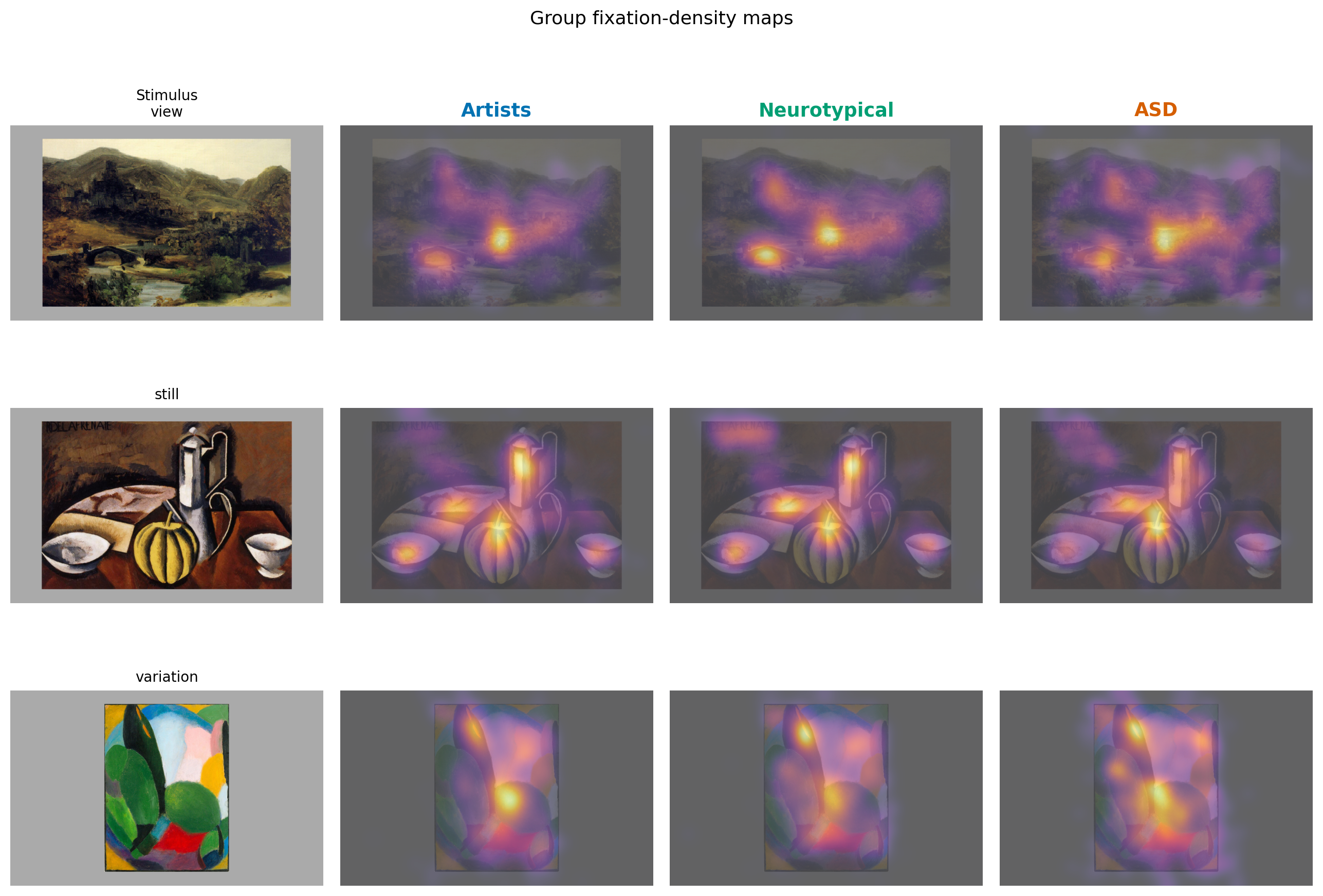
Figure 1 shows example group density maps; artist and neurotypical maps are visibly concentrated on shared regions, whereas ASD maps are more diffuse and shifted.
5.1 Spatial axis: artists \(\approx\) neurotypicals, ASD distinct↩︎
Table 1 and Fig. 2 summarise the directed spatial comparison. Two patterns stand out. First, the symmetric distribution metrics place artists and neurotypicals almost on top of each other
(art--typ \(\text{CC}=0.959\), \(\text{SIM}=0.856\)), while every pair involving ASD is lower and nearly identical to one another (ASD–Art\(\text{CC}=0.938\); ASD–Typ\(\text{CC}=0.937\)): the ASD density map is the odd one out, and about
equally distant from both other groups. Second, the directional location metrics show that ASD fixations are the hardest to predict: any group predicting ASD scores lowest (e.g. Art\(\rightarrow\)ASD\(\text{AUC}=0.873\), Typ\(\rightarrow\)ASD\(=0.876\)), whereas ASD as a predictor is only slightly worse than the third group. Absolute agreements are high across the board, all groups are drawn to the same strongly salient regions, so the effect is a modulation on top
of a large shared, stimulus-driven scaffold rather than the presence or absence of alignment.
| pair | AUC\(\uparrow\) | NSS\(\uparrow\) | CC\(\uparrow\) | SIM\(\uparrow\) | KL\(\downarrow\) | IG\(\uparrow\) |
|---|---|---|---|---|---|---|
| 0.908 | 2.094 | 0.959 | 0.856 | 0.092 | 0.980 | |
| 0.888 | 1.909 | 0.959 | 0.856 | 0.114 | 0.832 | |
| 0.902 | 2.035 | 0.937 | 0.822 | 0.156 | 0.866 | |
| 0.876 | 1.877 | 0.937 | 0.822 | 0.216 | 0.724 | |
| 0.879 | 1.852 | 0.938 | 0.831 | 0.171 | 0.724 | |
| 0.873 | 1.871 | 0.938 | 0.831 | 0.198 | 0.733 |
3.5pt
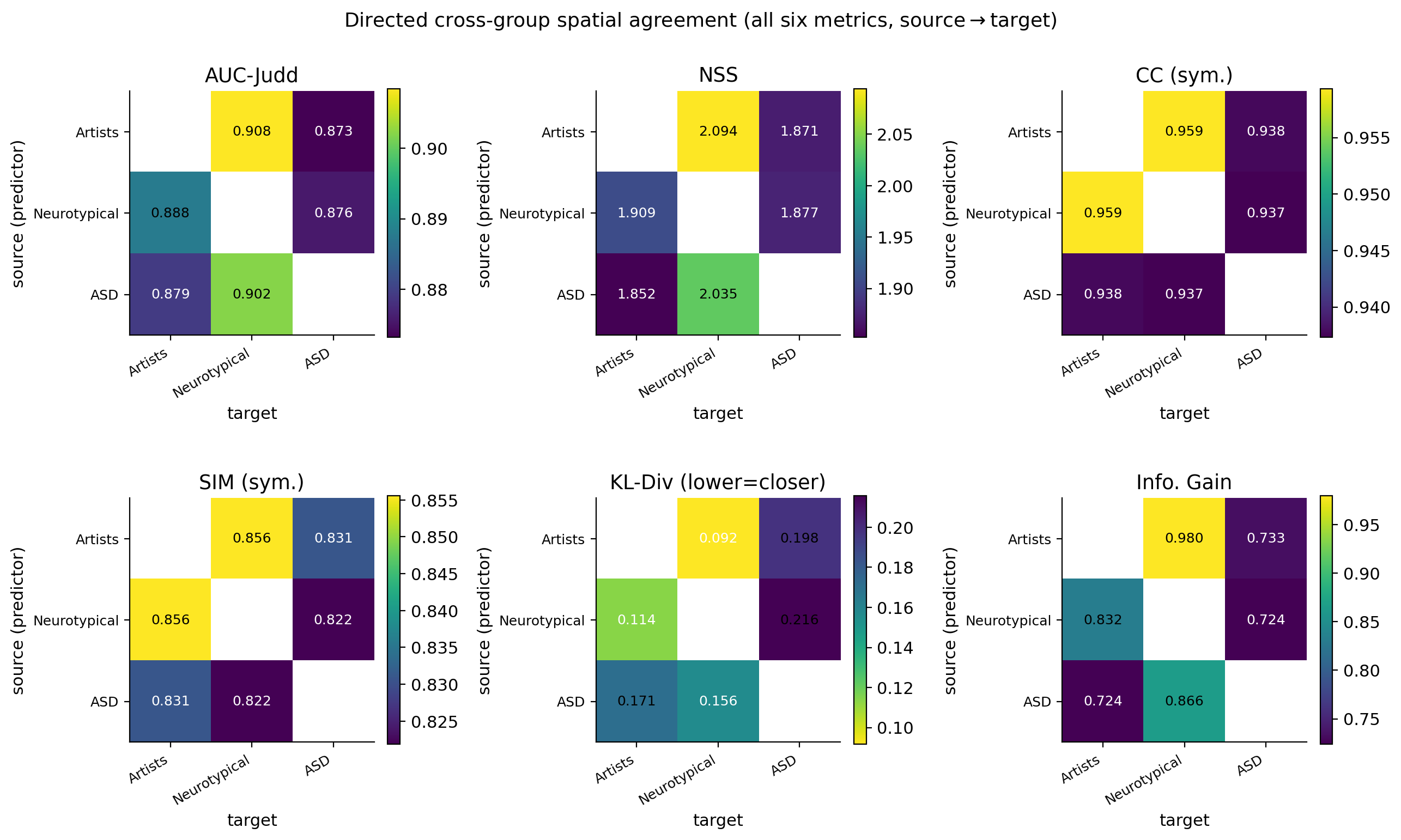
The primary contrast (ASD\(\rightarrow\)Artvs.ASD\(\rightarrow\)Typ) is significant on the directional metrics (AUC \(d=-1.65\), NSS \(d=-1.52\), IG \(d=-0.89\); all \(p<10^{-4}\)) but not on the symmetric ones (CC \(d=0.03\), \(p=0.88\); SIM \(d=0.34\), \(p=0.07\)). The directional difference reflects that neurotypical fixations are more predictable in general, not that ASD is selectively similar to either group, symmetrically, ASD is equidistant from artists and neurotypicals.
5.2 Per-scanpath features: ASD explores widely but briefly↩︎
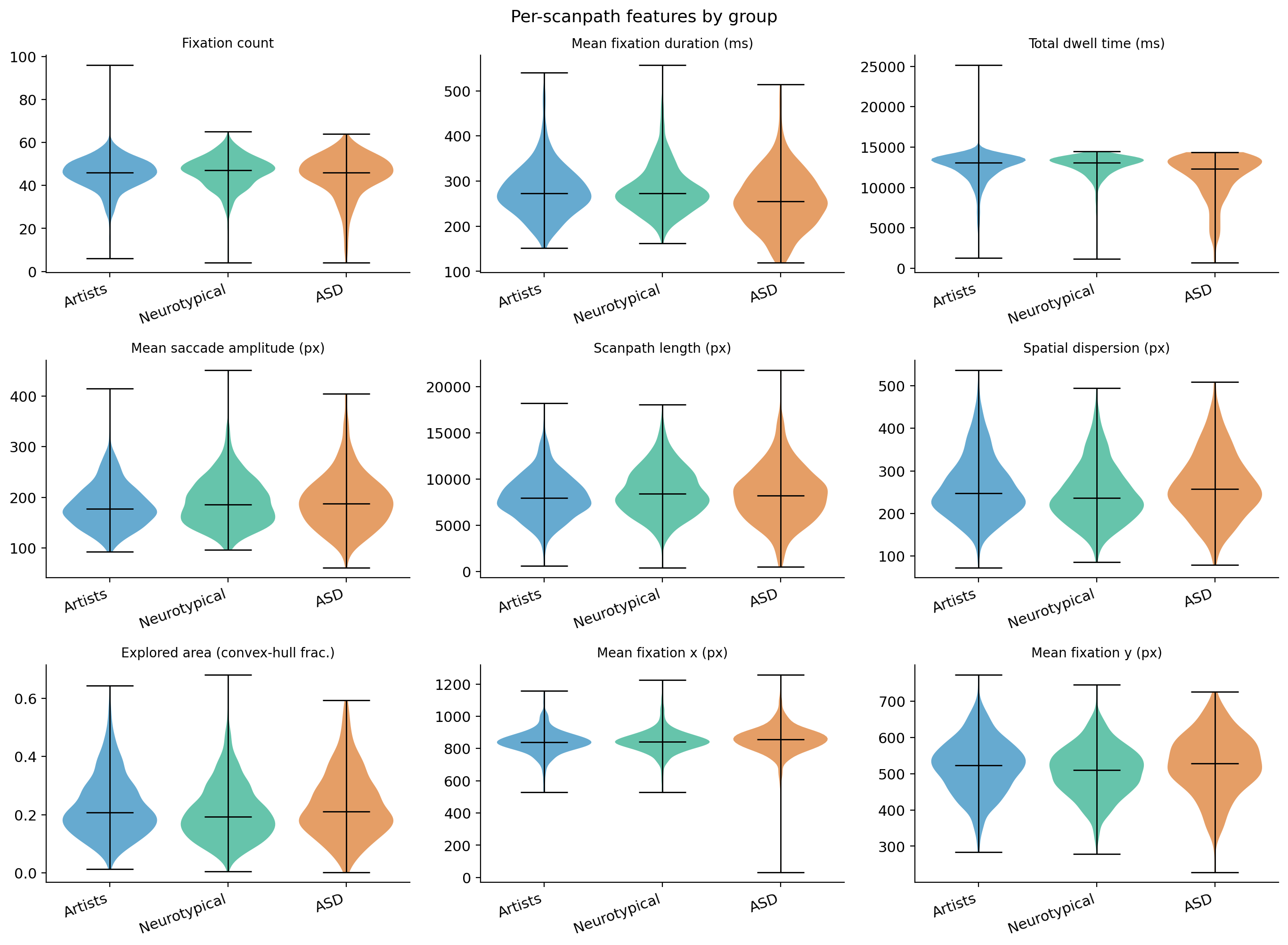
Table 2 reports per-scanpath features by group; all nine differ across groups (Kruskal–Wallis, \(p<0.03\); \(p<10^{-3}\) for seven of nine). ASD viewers make fixations that are significantly shorter (258 ms vs./281 ms; Holm \(p<10^{-4}\)) and accumulate less total dwell time, despite a similar number of fixations. Spatially, ASD scanpaths are more dispersed and cover a larger explored area than neurotypical ones (\(p<10^{-3}\)), matching artists, and are the least centre-biased (fixation centroid shifted right and downward, \(p<10^{-3}\)). In short (Fig. 3), ASD shares artists’ wide spatial exploration but couples it with a distinct temporal profile of shorter, less dwelling fixations.
| feature | \(p\) | |||
|---|---|---|---|---|
| Fixations | 45.3 | 46.2 | 44.6 | 0.02 |
| Dur.mean (ms) | 278.8 | 280.6 | 258.3 | \(<10^{-4}\) |
| Total dwell (ms) | 12388 | 12680 | 11318 | \(<10^{-4}\) |
| Saccade amp.(px) | 183.6 | 191.4 | 192.6 | 0.003 |
| Scanpath length (px) | 8148 | 8670 | 8373 | \(<10^{-3}\) |
| Dispersion (px) | 261.3 | 246.7 | 265.5 | \(<10^{-4}\) |
| Explored area (hull) | 0.23 | 0.21 | 0.23 | \(10^{-4}\) |
| Centroid \(x\) (px) | 839.6 | 843.9 | 856.0 | \(10^{-4}\) |
| Centroid \(y\) (px) | 520.7 | 507.3 | 526.5 | \(<10^{-4}\) |
4pt
5.3 Temporal axis: ASD scanpaths are the most idiosyncratic↩︎
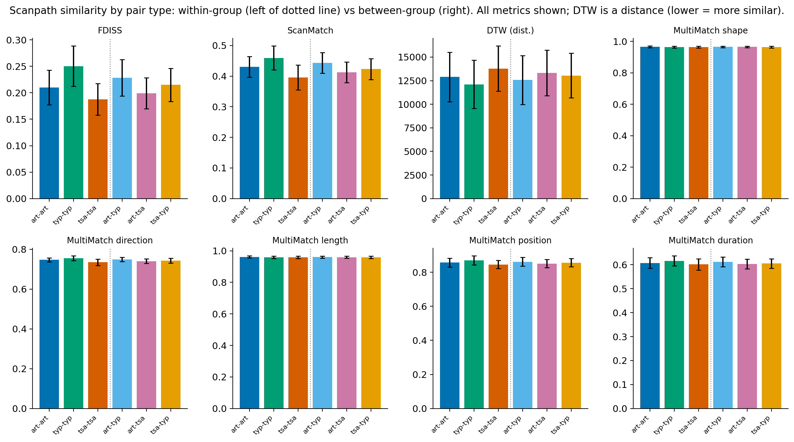
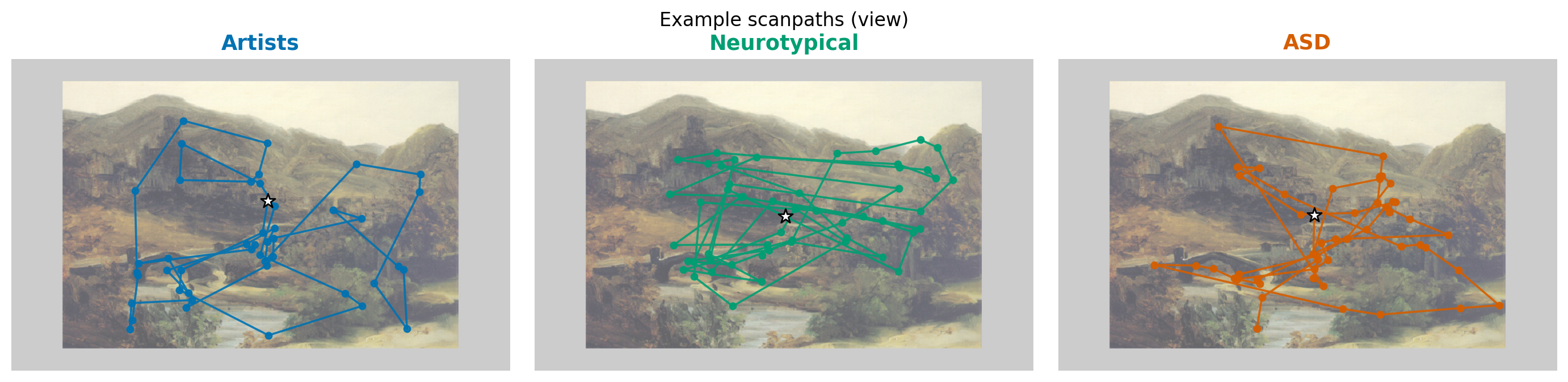
Table 3 reports within- and between-group scanpath similarity, and the ordering is remarkably consistent across MultiMatch, ScanMatch, FDISS and DTW (Fig. 4). Figure 5 illustrates the qualitative difference with one representative scanpath per group. Three findings mirror and extend the spatial axis.
Within-group cohesion. Neurotypical scanpaths are the most self-consistent, artists intermediate, and ASD the least (tsa-tsa lowest on every metric: FDISS 0.188 vs./0.250; ScanMatch 0.395 vs./0.460; DTW largest
distance). Autistic viewers are as different from one another as they are from other groups, their “group-specific” pattern is better described as a set of heterogeneous individual styles than a single shared one.
Between-group alignment. art--typ is the most alignable between-group pair, significantly exceeding both art--tsa (FDISS \(d=+2.32\)) and tsa--typ (FDISS \(d=+1.01\); all \(p<10^{-3}\)), reinforcing the artist–neurotypical convergence seen spatially. The ordering is stimulus-general rather than driven by a few paintings: by FDISS,
art--typ is the most alignable between-group pair on 25 of 30 paintings, and tsa--typ exceeds art--tsa on 29 of 30 (spatially, Art–Typ has the highest CC
on 26 of 30).
Not selectively artist-like. The key temporal contrast (art--tsa vs.tsa--typ) is significant on every metric, and in the direction opposite to an “ASD-is-artist-like” hypothesis: ASD scanpaths are marginally
more similar to neurotypical than to artist ones (FDISS \(d=-1.99\), ScanMatch \(d=-0.98\), DTW \(d=+0.86\), MultiMatch-position \(d=-1.41\); all \(p<0.002\)).
| pair | FDISS\(\uparrow\) | ScanM.\(\uparrow\) | DTW\(\downarrow\) | MM-pos\(\uparrow\) |
|---|---|---|---|---|
| art-art | 0.210 | 0.430 | 12888 | 0.857 |
| typ-typ | 0.250 | 0.460 | 12114 | 0.869 |
| tsa-tsa | 0.188 | 0.395 | 13781 | 0.846 |
| art-typ | 0.228 | 0.443 | 12569 | 0.862 |
| art-tsa | 0.199 | 0.413 | 13318 | 0.851 |
| tsa-typ | 0.215 | 0.423 | 13047 | 0.856 |
4pt
6 Stimulus Properties and Low-Level Determinants of Gaze↩︎
Having established the group ordering in space and time, we now characterise the stimuli themselves and the low-level and individual-level structure of gaze. Table 4 consolidates the group contrasts that recur below.
| measure | KW \(p\) | |||
|---|---|---|---|---|
| Central distance (norm.) | 0.41 | 0.39 | 0.42 | \(<10^{-4}\) |
| Saccade amplitude (°) | 3.61 | 3.80 | 3.56 | \(<10^{-10}\) |
| Pupil diameter (mm) | 4.46 | 4.93 | 4.90 | \(<10^{-300}\) |
| On-painting fraction | 0.95 | 0.97 | 0.94 | — |
| IOC (CC) | 0.67 | 0.74 | 0.61 | \(<10^{-5}\) |
5pt
6.1 Stimulus image properties↩︎
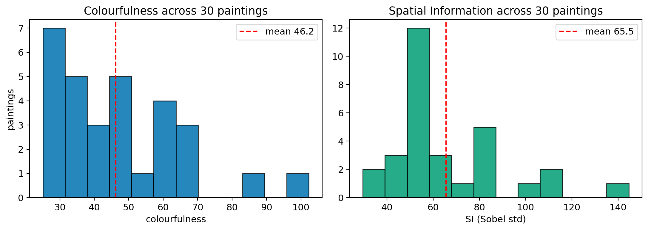
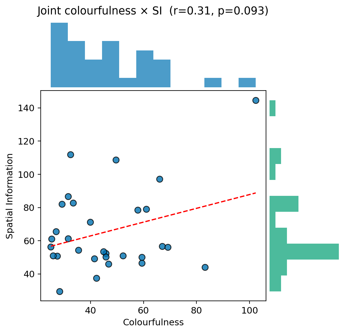
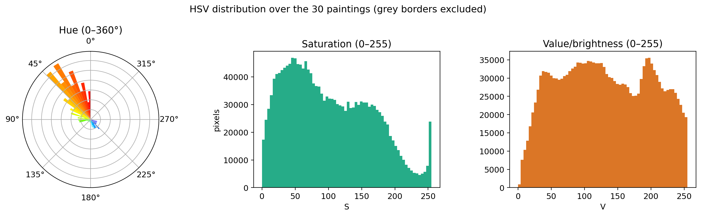
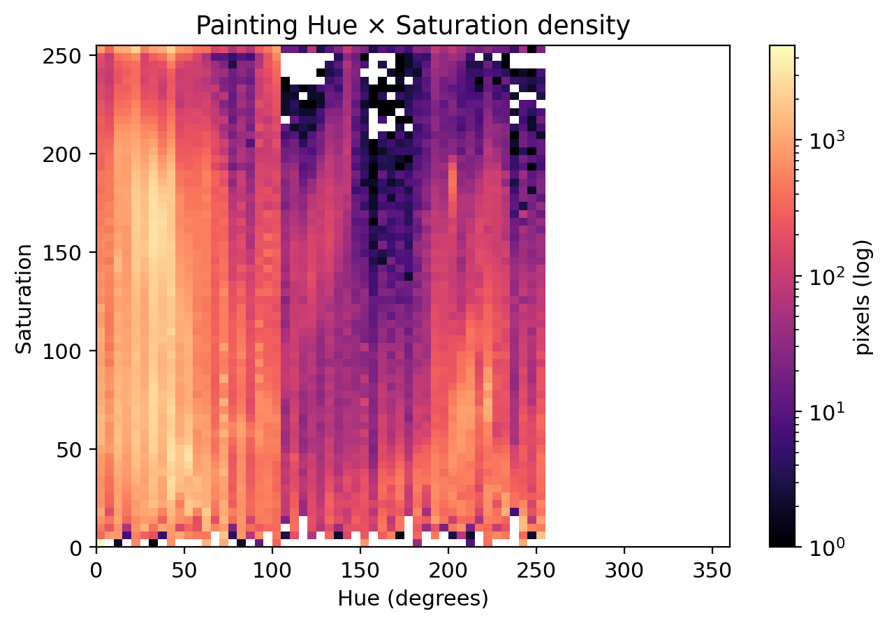
We first quantify the paintings themselves on content pixels only, having removed the uniform grey letterbox (RGB 170,170,170) in which each image was displayed. Per painting we compute colourfulness (Hasler–Süsstrunk) and spatial information (SI; the standard deviation of the Sobel gradient of luminance, ITU-T P.910). The set spans a wide range (colourfulness \(46.2\pm18.8\), range \(25{-}102\); SI \(65.5\pm25.0\), range \(30{-}145\); Fig. 6, Table 5). The two properties are only weakly and non-significantly correlated (\(r=0.31\), \(p=0.09\); Fig. 7), so colour richness and edge/detail density are largely independent axes of stimulus complexity here. The palette is warm-dominated, with hue mass concentrated in reds–oranges–yellows, mid-range saturation, and a broad brightness distribution (Fig. 8; Hue\(\times\)Saturation density in Supplement Fig. 18).
| Colourf. | SI | Hue | Sat. | Val. | |
|---|---|---|---|---|---|
| mean | 46.2 | 65.5 | 48.4 | 101.0 | 131.2 |
| SD | 18.8 | 25.0 | 20.3 | 31.3 | 28.9 |
6.2 Saccadic dynamics↩︎
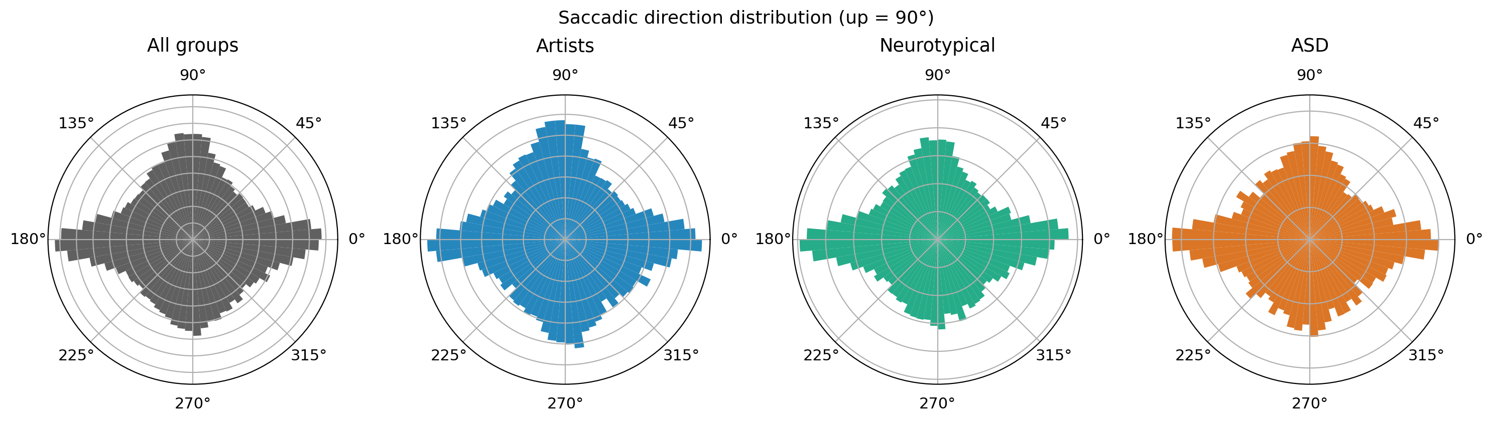
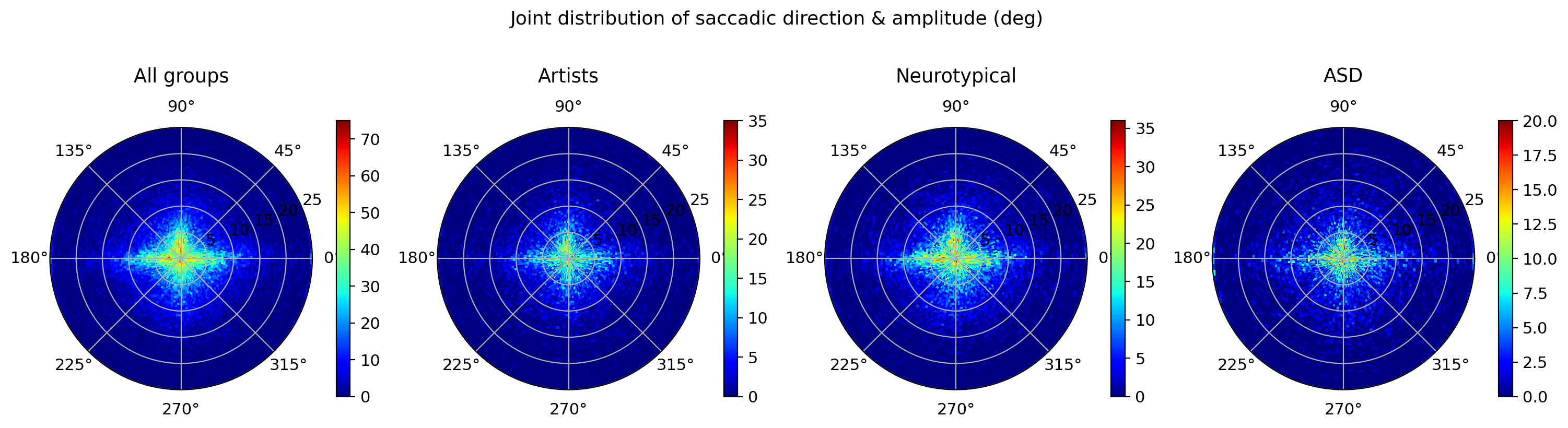
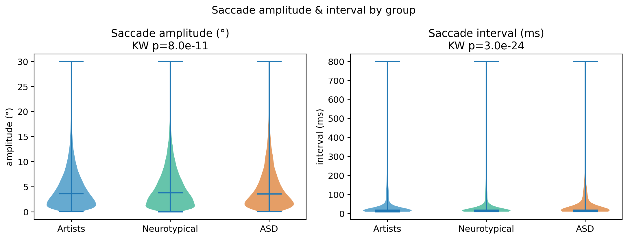
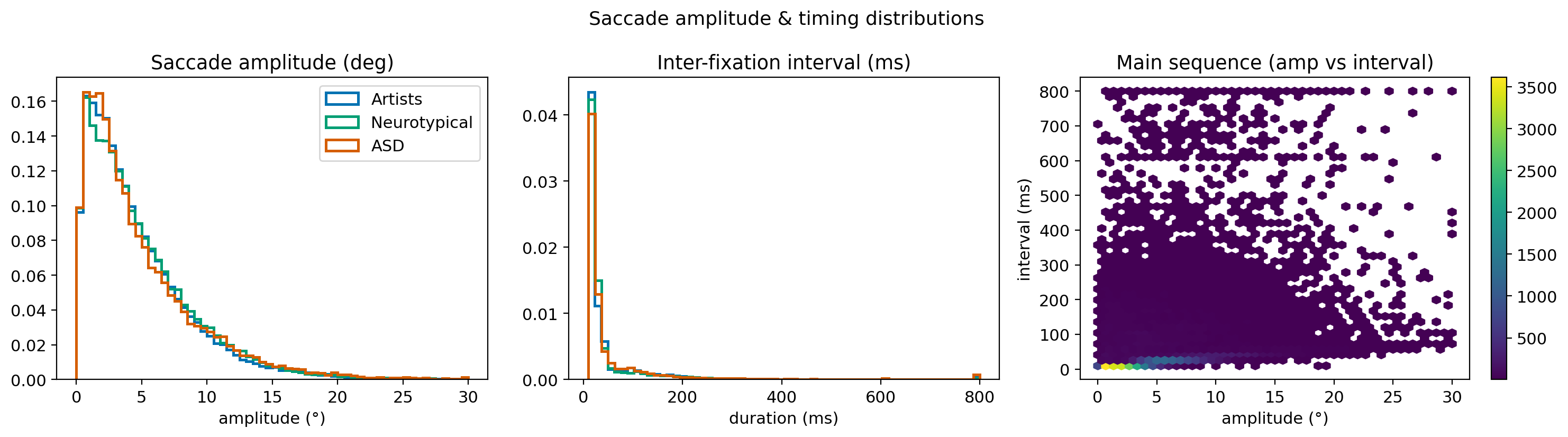
Saccades (transitions between consecutive fixations) are strongly anisotropic: the direction distribution is dominated by the horizontal axis in all three groups (Fig. 9), and the joint direction × amplitude distribution (Fig. 10) shows the characteristic horizontal "cross" with mass concentrated at small amplitudes. Amplitudes differ by group (median \(3.8^\circ\) Typ, \(3.6^\circ\) Art, \(3.6^\circ\) ASD; Kruskal–Wallis \(p=8\times10^{-11}\); Fig. 11): neurotypical observers make the largest saccades, consistent with their broader, more centre-anchored scanning, whereas ASD makes the smallest. The amplitude–interval main sequence is shown in Supplement Fig. 19.
6.3 Spatial fixation distribution and central bias↩︎
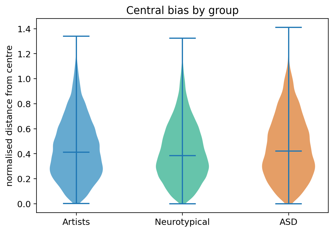
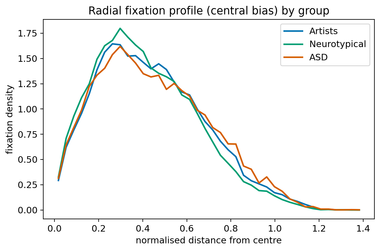
Pooling all \(95{,}282\) fixations reveals a strong central bias in every group (Fig. 12), but its strength differs: neurotypical fixations are the most centre-anchored and ASD the least (median normalised distance from centre \(0.39\) Typ \(<0.41\) Art \(<0.42\) ASD; Kruskal–Wallis \(p<10^{-4}\); pairwise Holm \(p<10^{-4}\) for both ASD/Typ and Art/Typ; Fig. 13, radial profile in Supplement Fig. 20). ASD observers also land off the painting (on the grey surround) more often than the others (\(4.3\%\) vs.\(3.5\%\) neurotypical). The reduced central bias converges with the wider spatial dispersion reported in Section 5.

6.4 Colour selection at fixation↩︎
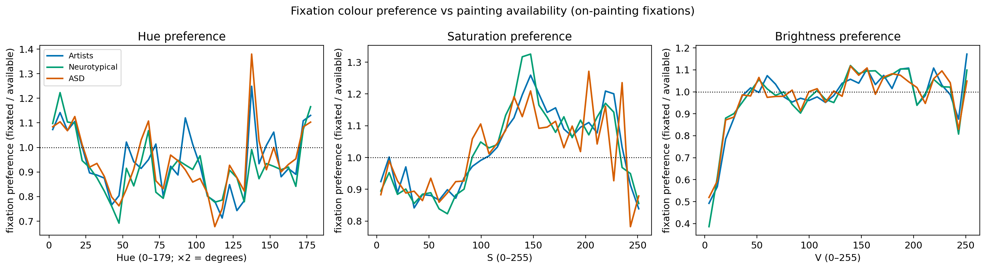
Sampling each fixation’s painting pixel shows that gaze is not colour-neutral: in all three groups, fixated pixels are significantly more saturated (median \(103\) vs.available \(92\); Mann–Whitney \(p<10^{-140}\)) and slightly brighter (median \(133\) vs.\(128\); \(p<10^{-28}\)) than the painting average (Fig. 14, per-hue preference in Supplement Fig. 21). The preference for saturated, luminous regions is shared across groups, indicating a common low-level colour driver of attention on top of the group-specific spatial and temporal differences.

6.5 Pupillometry↩︎
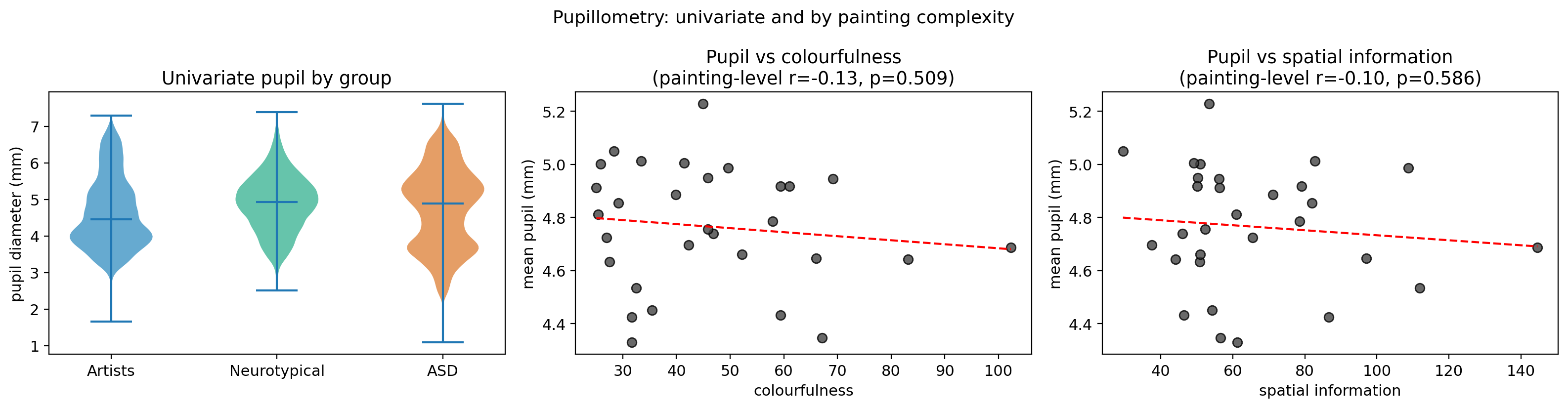
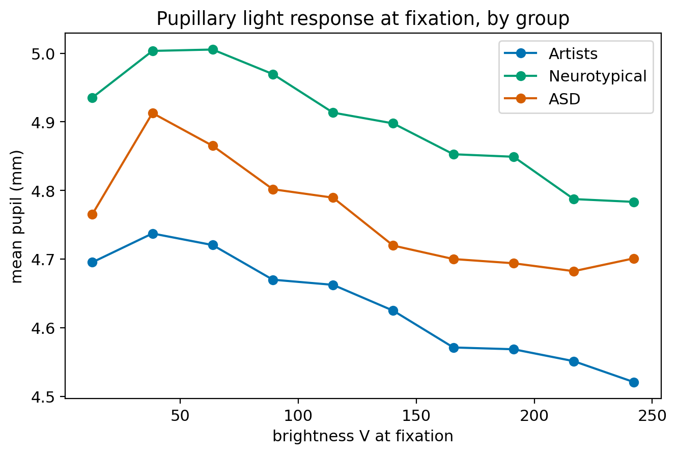
Mean pupil diameter differs by group, with artists showing the smallest pupils (\(4.46\) mm) and neurotypical and ASD observers larger and similar (\(4.93\)/\(4.90\) mm; Fig. 15). Pupil size tracks the brightness at the fixated location in the expected direction of the pupillary light response — pupils constrict on brighter regions — in every group (Art \(r=-0.07\), Typ \(r=-0.09\), ASD \(r=-0.06\); all \(p<10^{-16}\); Fig. 16), with the response weakest in ASD. At the painting level, pupil size is only weakly related to colourfulness and SI (Fig. 15, right), so the dominant modulator of pupil here is local luminance rather than global stimulus complexity.
6.6 Inter-observer congruency↩︎
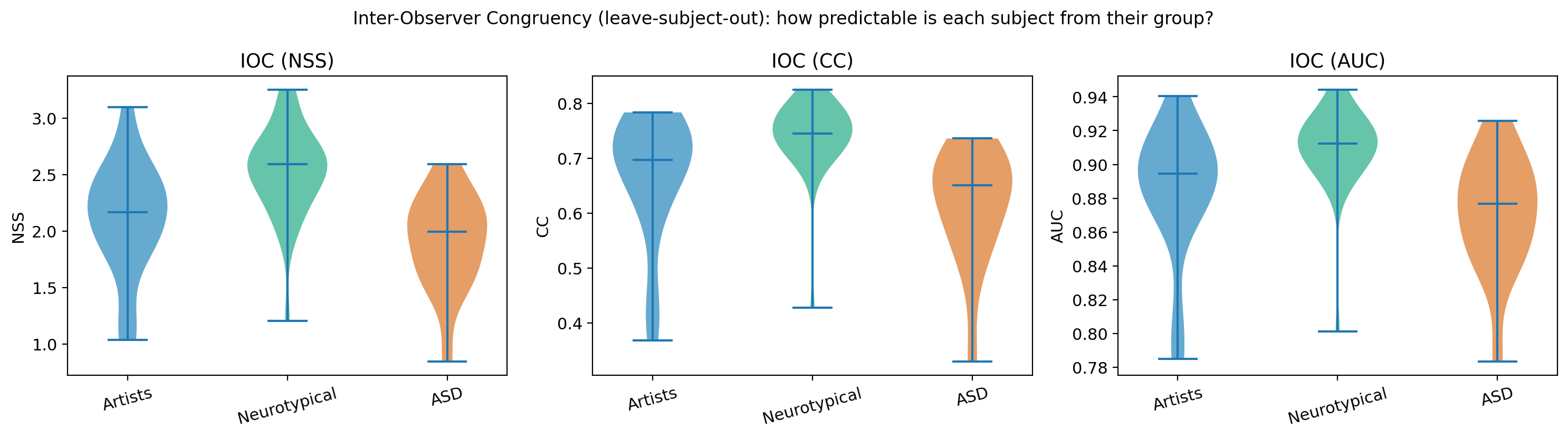
Finally, a leave-one-subject-out analysis quantifies how predictable each observer is from the rest of their own group: each subject’s fixations are scored (NSS, CC, AUC-Judd) against the density map of the remaining same-group members. Congruency is ordered Neurotypical \(>\) Artists \(>\) ASD on every measure (CC \(0.74>0.67>0.61\); Kruskal–Wallis \(p<10^{-5}\), \(\varepsilon^2\approx0.34\); Table 6, Fig. 17). Neurotypical observers are significantly more congruent than both other groups, and ASD the least (Holm-corrected CC: Typ\(>\)ASD \(p<10^{-3}\), Typ\(>\)Art \(p=0.004\), Art\(>\)ASD \(p=0.025\)). This is an entirely independent confirmation, at the individual level, of the within-group scanpath result in Section 5: autistic viewing is not merely different from the other groups, it is the least internally consistent.
| group | NSS | CC | AUC |
|---|---|---|---|
| Artists | \(2.12\pm0.50\) | \(0.67\pm0.11\) | \(0.885\pm0.039\) |
| Neurotypical | \(\mathbf{2.53\pm0.40}\) | \(\mathbf{0.74\pm0.07}\) | \(\mathbf{0.910\pm0.025}\) |
| ASD | \(1.91\pm0.43\) | \(0.61\pm0.11\) | \(0.871\pm0.035\) |
7 Discussion↩︎
7.0.0.1 A convergent artist–neurotypical baseline.
Across ten metrics and both axes, artists and neurotypicals are strikingly similar: near-identical density maps and the most alignable scanpaths. Under brief, untasked free-viewing, much of what both groups do is a shared, conspicuity-driven exploration of the same compositional structure, and expertise modulates gaze on top of that scaffold rather than replacing it. The strong artist–neurotypical alignment should thus be read as evidence of shared bottom-up looking under these conditions, not as proof that expertise leaves gaze unchanged; a longer or explicitly analytic task would be expected to widen the gap.
7.0.0.2 A spatial–temporal dissociation in ASD.
The central new result is that autistic viewing cannot be summarised by a single scalar of “similarity.” Spatially, ASD gaze resembles artists: widely dispersed, covering more of the canvas, and less centre-biased than neurotypical gaze. Temporally, it is distinct from both: fixations are shorter, dwell is lower, and the ordered sequences are the least self-consistent of any group. The same-where, different-how pattern is consistent with a detail-focused, locally biased style [7], [8] and with gaze being tied more to low-level salience than to semantic structure [9]: rapid, broadly distributed sampling produces wide spatial coverage but short, idiosyncratic temporal trajectories. Critically, this is not an exaggerated form of expert looking, on no metric is ASD selectively artist-like.
7.0.0.3 Heterogeneity and personalised models.
That tsa-tsa is the least cohesive cell indicates the ASD “profile” is partly an aggregate of divergent individual strategies. This has a direct methodological consequence: saliency and scanpath models for art are trained and evaluated
against neurotypical fixations [10]–[12],
and our results imply that such models predict artist gaze well but ASD gaze poorly, because viewer population is a latent variable they ignore. Treating population identity, and, given the heterogeneity, individual identity, as an explicit conditioning
variable is a concrete direction, especially for accessibility settings where the intended viewer is by definition not neurotypical. The directed two-axis framework here offers a ready way to audit such models: not only how well a model predicts aggregate
gaze, but whose gaze, and whether it reproduces the temporal as well as the spatial signature. The leave-subject-out inter-observer congruency (Section 6.6) makes the heterogeneity concrete and quantitative: ASD observers are the least predictable
from their own group on every measure, independently confirming the aggregate scanpath result at the level of individual subjects.
7.0.0.4 Low-level drivers beneath the group differences.
The low-level analyses locate the group effects on a shared perceptual substrate. All three groups fixate more saturated and brighter pixels than the painting average, saccade predominantly along the horizontal, and show the pupillary light response, so a common bottom-up machinery is engaged throughout. The group differences ride on top of it: neurotypical gaze is the most centre-anchored and makes the largest saccades, artists sit between, and ASD is the least centre-biased, makes the smallest saccades, and most often leaves the painting altogether. That colourfulness and spatial information are only weakly correlated (\(r=0.31\)) yet neither strongly modulates pupil size suggests that, under brief free-viewing, local luminance rather than global stimulus complexity is the dominant low-level driver, and that the group signature is carried by how gaze is deployed over that substrate rather than by differential sensitivity to stimulus complexity.
7.0.0.5 A reusable two-axis auditing framework.
Beyond the specific findings, the analysis itself is a contribution. Casting group comparison as a directed problem, one population’s map or scanpath used to predict another’s gaze, turns any saliency or scanpath metric into a measure of cross-group (dis)similarity, and pairing a spatial axis with a temporal one exposes structure that either alone would miss. Here, a purely spatial analysis would have reported that ASD “explores like an artist,” while a purely temporal one would have missed the shared spatial breadth; only the two together reveal the dissociation. The same framework generalises directly to model auditing: a gaze model can be scored not only by aggregate accuracy but by whose gaze it reproduces and on which axis, and its directional (a)symmetries, for instance, that every group predicts ASD fixations better than ASD predicts theirs, become first-class, testable quantities. Because the pipeline applies one identical fixation-extraction rule to all groups and reports ten complementary metrics with effect sizes and power, it offers a transparent, reproducible template for characterising attentional differences in other clinical or expert populations.
8 Limitations↩︎
Several limitations bound interpretation. The ASD sample is modest (\(n=15\)) and the groups are not matched on age or sex, so group, age, sex and expertise are partially confounded. Absolute cross-group similarities are high because pooled maps over many participants are smooth and dominated by shared stimulus structure; our conclusions are therefore comparative, about the ordering of group pairings, rather than statements about absolute predictive quality. Density maps pool participants and discard individual variability on the spatial axis (the temporal axis, computed per participant, partially addresses this). Fixation extraction uses one dispersion rule; while applied uniformly, different thresholds would shift absolute counts (we report a robustness check in the supplement). Finally, we do not yet include a computational bottom-up saliency baseline or object/face/semantic annotations that would let us separate stimulus-driven overlap from genuinely group-specific strategy.
9 Conclusion & Future Work↩︎
We presented a directed, two-axis (spatial and temporal), metric-grounded comparison of free-viewing gaze on paintings across autistic, artist and neurotypical observers. Artists and neurotypicals converge in both space and time; ASD gaze is distinct on both axes, exhibits a spatial–temporal dissociation (artist-like spatial breadth, a unique temporal signature), is the most idiosyncratic group, and is not selectively artist-like. Future work should scale the sample and match groups on demographics; move from pooled to individual- and subgroup-level analyses to characterise ASD heterogeneity; add bottom-up and semantic baselines to separate stimulus-driven from group-specific gaze; and develop population- and person-conditioned models of aesthetic attention, evaluated on both axes, for accessibility applications.
Declarations↩︎
Ethics. The study was conducted in accordance with the Declaration of Helsinki. Participation was voluntary and informed consent was obtained from all participants. Data were anonymised before analysis and no personally identifiable information was collected or retained.
Data and code availability. Analysis code, the extracted fixation/scanpath tables, and all per-stimulus results are released at https://github.com/kmamine/TSA-Art-Typ-results. Raw eye-tracking recordings are available from the corresponding author on reasonable request, subject to the participants’ consent terms.
Author contributions (CRediT). M.A.K.: conceptualisation, methodology, software, formal analysis, writing – original draft. D.S., R.J., O.L.: investigation, data curation. M.T., A.C.: methodology, software, writing – review & editing. C.W., E.H.-D., S.M.-K.: investigation, resources, validation. N.A.-H.: conceptualisation, supervision, funding acquisition, writing – review & editing.
Conflict of interest. The authors declare no competing interests.
Funding. This work received no specific grant from funding agencies in the public, commercial, or not-for-profit sectors.
Generative-AI usage disclosure. An AI coding assistant (Claude, Anthropic) was used under author supervision to help implement the analysis pipeline, run the statistical computations, and draft and format the manuscript. All methods, results, and interpretations were verified by the authors, who take full responsibility for the content. No text or citation was included without author verification.
Supplementary Material
Divergent Gaze Patterns in Artistic Viewing: Spatial and Temporal Signatures
This supplement provides the full statistical tables underlying the main results (the main text reports condensed versions), an additional qualitative figure, and the exact methodological parameters and software versions needed to reproduce the analysis. All tables are regenerated by the released code from the raw SMI exports.
10 Fixation extraction and dataset details↩︎
Fixations were extracted uniformly for all groups from the median-smoothed, averaged binocular point of regard using dispersion-threshold identification (IDT) [20]. Parameters: median-filter window \(=15\) samples (\(\approx\)30 ms at 500 Hz); down-sampling factor \(=3\) (500 \(\approx\)167 Hz) for tractable IDT; minimum fixation duration \(=100\) ms; maximum duration \(=1500\) ms; maximum dispersion \(=90\) px (\(\approx 2.3^{\circ}\) at 39 px/deg). Scanpaths with fewer than four fixations were discarded. The final set contains 95,282 fixations in 2,091 scanpaths (Artists 712, Neurotypical 940, ASD 439), mean 45.6 fixations per scanpath and mean fixation duration \(\approx\)200 ms. The vendor per-sample event labels were not used: on this recording they label \(\sim\)47% of samples as saccade, which fragments fixations and, because the fragmentation depends on per-participant tracking quality, would confound group comparison.
Spatial density maps were built on a \(210\times131\) grid (screen down-scaled \(8\times\)), with a Gaussian kernel \(\sigma=40\) px (\(\approx1^{\circ}\)); the Information-Gain baseline is a centred Gaussian prior. Scanpath metrics used a foveal radius of \(1^{\circ}\) (39 px) for FDISS and a \(12\times8\) ScanMatch grid.
11 Spatial axis: full ASD selectivity contrast↩︎
Table 7 gives the paired contrast ASD\(\rightarrow\)Artvs. ASD\(\rightarrow\)Typover the 30 paintings for all six metrics. The directional metrics (AUC, NSS, IG) differ significantly (ASD predicts neurotypical fixations better than artist fixations), but the symmetric distribution metrics (CC, SIM) do not: ASD is spatially equidistant from the two groups.
| metric | mean\(_a\) | mean\(_b\) | diff | \(t\) | \(p\) | Cohen’s \(d\) | power |
|---|---|---|---|---|---|---|---|
| AUC | 0.879 | 0.902 | \(-0.023\) | \(-9.06\) | \(<10^{-4}\) | \(-1.65\) (L) | 1.00 |
| NSS | 1.853 | 2.035 | \(-0.183\) | \(-8.30\) | \(<10^{-4}\) | \(-1.52\) (L) | 1.00 |
| CC | 0.938 | 0.937 | \(+0.001\) | \(0.15\) | \(0.884\) | \(+0.03\) (T) | 0.05 |
| SIM | 0.831 | 0.822 | \(+0.009\) | \(1.87\) | \(0.072\) | \(+0.34\) (S) | 0.44 |
| KL | 0.171 | 0.156 | \(+0.015\) | \(1.28\) | \(0.211\) | \(+0.23\) (S) | 0.24 |
| InfoGain | 0.724 | 0.866 | \(-0.141\) | \(-4.89\) | \(<10^{-4}\) | \(-0.89\) (L) | 1.00 |
12 Temporal axis: full similarity table↩︎
Table 8 reports all four measures and the five MultiMatch sub-dimensions for every pair type (mean over paintings; standard deviations are in the released CSV). The MultiMatch shape, length and direction sub-dimensions saturate near ceiling for the \(\sim\)46-fixation scanpaths here and are therefore weakly discriminative; FDISS, ScanMatch, DTW and MultiMatch-position carry the group structure.
| pair | FDISS | SM | DTW | MM-shape | MM-dir | MM-len | MM-pos | MM-dur | |
|---|---|---|---|---|---|---|---|---|---|
| art-art | 0.210 | 0.430 | 12888 | 0.966 | 0.747 | 0.961 | 0.857 | 0.607 | |
| typ-typ | 0.250 | 0.460 | 12114 | 0.965 | 0.755 | 0.959 | 0.869 | 0.616 | |
| tsa-tsa | 0.188 | 0.395 | 13781 | 0.964 | 0.735 | 0.959 | 0.846 | 0.601 | |
| art-typ | 0.228 | 0.443 | 12569 | 0.965 | 0.750 | 0.960 | 0.862 | 0.612 | |
| art-tsa | 0.199 | 0.413 | 13318 | 0.965 | 0.740 | 0.960 | 0.851 | 0.603 | |
| tsa-typ | 0.215 | 0.423 | 13047 | 0.964 | 0.743 | 0.959 | 0.856 | 0.605 |
4.5pt
Table 9 gives the temporal primary contrast (art-tsa vs.tsa-typ); every metric is significant and in the direction of ASD being closer to neurotypical than to artist. Table 10 confirms the art-typ pair is the most alignable, significantly exceeding both ASD-involving between-group pairs.
| metric | mean\(_a\) | mean\(_b\) | \(t\) | \(p\) | Cohen’s \(d\) | power |
|---|---|---|---|---|---|---|
| FDISS | 0.199 | 0.215 | \(-10.92\) | \(<10^{-4}\) | \(-1.99\) (L) | 1.00 |
| ScanMatch | 0.413 | 0.423 | \(-5.35\) | \(<10^{-4}\) | \(-0.98\) (L) | 1.00 |
| DTW | 13318 | 13047 | \(4.71\) | \(10^{-4}\) | \(+0.86\) (L) | 1.00 |
| MM-shape | 0.965 | 0.964 | \(3.47\) | \(0.002\) | \(+0.63\) (M) | 0.92 |
| MM-direction | 0.740 | 0.743 | \(-3.80\) | \(<10^{-3}\) | \(-0.69\) (M) | 0.96 |
| MM-length | 0.960 | 0.959 | \(3.99\) | \(<10^{-3}\) | \(+0.73\) (M) | 0.97 |
| MM-position | 0.851 | 0.856 | \(-7.73\) | \(<10^{-4}\) | \(-1.41\) (L) | 1.00 |
| MM-duration | 0.603 | 0.605 | \(-1.63\) | \(0.115\) | \(-0.30\) (S) | 0.35 |
| vs.art-tsa | vs.tsa-typ | |||
|---|---|---|---|---|
| 2-3(lr)4-5 metric | \(d\) | \(p\) | \(d\) | \(p\) |
| FDISS | \(+2.32\) | \(<10^{-4}\) | \(+1.01\) | \(<10^{-4}\) |
| ScanMatch | \(+1.72\) | \(<10^{-4}\) | \(+1.21\) | \(<10^{-4}\) |
| DTW | \(-1.11\) | \(<10^{-4}\) | \(-0.74\) | \(<10^{-3}\) |
| MM-direction | \(+1.27\) | \(<10^{-4}\) | \(+0.80\) | \(10^{-4}\) |
| MM-position | \(+1.43\) | \(<10^{-4}\) | \(+0.80\) | \(10^{-4}\) |
| MM-duration | \(+1.20\) | \(<10^{-4}\) | \(+0.71\) | \(<10^{-3}\) |
13 Per-scanpath features: pairwise ASD contrasts↩︎
Table 11 reports Holm-corrected Mann–Whitney contrasts of ASD vs. the other two groups (rank-biserial correlation, rbc; positive = first group higher). ASD has shorter fixations and less dwell than both groups, and greater dispersion, larger explored area and a less centred fixation centroid than neurotypicals.
| feature | contrast | med\(_1\) | med\(_2\) | rbc (\(p\)) |
|---|---|---|---|---|
| Dur.mean | art / tsa | 272.8 | 254.5 | \(-0.19\;(<10^{-4})\) |
| tsa / typ | 254.5 | 272.7 | \(+0.21\;(<10^{-4})\) | |
| Total dwell | art / tsa | 13053 | 12338 | \(-0.20\;(<10^{-4})\) |
| tsa / typ | 12338 | 13074 | \(+0.26\;(<10^{-4})\) | |
| Dispersion | tsa / typ | 257.2 | 235.8 | \(-0.15\;(<10^{-3})\) |
| Explored area | tsa / typ | 0.211 | 0.192 | \(-0.12\;(<10^{-3})\) |
| Centroid \(x\) | art / tsa | 838.9 | 856.5 | \(+0.14\;(10^{-4})\) |
| Centroid \(y\) | tsa / typ | 527.9 | 510.0 | \(-0.16\;(<10^{-4})\) |
| Saccade amp. | art / tsa | 177.7 | 187.3 | \(+0.09\;(0.02)\) |
14 Robustness to the fixation-extraction threshold↩︎
Because IDT requires a dispersion threshold, we re-ran the full extraction at a stricter (\(60\) px) and a looser (\(120\) px) value, bracketing the \(90\) px used in the main text, and recomputed the headline quantities (Table 12). Absolute fixation counts and durations shift with the threshold, as expected, but every conclusion is preserved
at all three settings: ASD has the shortest mean fixation duration; within-group cohesion is always ordered typ-typ\(>\)art-art\(>\)tsa-tsa; and
the ASD selectivity contrast art-tsa\(<\)tsa-typ holds with a large effect (\(d\!\le\!-1.95\), \(p<10^{-10}\)). The headline
findings are therefore not artefacts of a particular threshold choice.
| quantity | \(60\) px | \(90\) px (main) | \(120\) px |
|---|---|---|---|
| Fixations / scanpath | 50.1 | 45.6 | 41.8 |
| Dur.art / typ / tsa (ms) | 232/226/214 | 279/281/258 | 313/308/288 |
| Cohesion art / typ / tsa | .22/.26/.19 | .21/.25/.19 | .20/.24/.18 |
| art-tsa / tsa-typ | .204/.222 | .199/.215 | .191/.207 |
| Contrast \(d\) (\(p\)) | \(-2.08\;(10^{-12})\) | \(-1.99\;(10^{-11})\) | \(-1.95\;(10^{-11})\) |
4pt
15 Additional low-level figures↩︎
This section collects the supporting figures referenced from Section 6 (stimulus properties and low-level determinants of gaze).

16 Software and reproducibility↩︎
Analyses were run in Python 3.12 with: eyefeatures 2.0.2 (IDT extraction), scanpath-nlp-metrics 0.0.1 (MultiMatch, ScanMatch, DTW), fdiss 0.1.0 (FDISS), numpy 1.26, pandas 2.2,
scipy 1.14, statsmodels 0.14, opencv 4.11, and matplotlib 3.8. The pipeline (fixation extraction, spatial metrics, scanpath comparison, feature extraction, statistics, figures) and all per-stimulus
outputs are released at https://github.com/kmamine/TSA-Art-Typ-results.