Subjective Risk Decomposition:
A New View for Uncertainty Quantification
July 16, 2026
Abstract
We present a novel viewpoint for uncertainty quantification. Uncertainty measures are not primitives, in need of axioms and argumentation, but instead consequences, of higher-level modeling decisions. We show how epistemic and aleatoric uncertainty measures can be derived via decomposition of a subjective risk, based on a strictly proper loss. Reverse cross-entropy provides a prominent example, where decomposition recovers the classic information-theoretic uncertainty terms. The same approach recovers numerous measures previously proposed across the UQ literature, providing them a common theoretical foundation. From a practical point of view, this suggests a new approach to UQ: given a modeling scenario and strictly proper loss, the corresponding epistemic and aleatoric terms are induced by the subjective-risk decomposition. We then extend our view to learning theory: we introduce and analyze subjective risk analogues of excess risk, approximation error and estimation error, and identify the connections to UQ. We consider this a first step towards a full learning-theoretic framework for uncertainty quantification.
epistemic, aleatoric, subjective risk, bias–variance, mutual information.
1 Introduction↩︎
A popular framework for uncertainty quantification is the aleatoric/epistemic decomposition introduced by [1]. This adopts a Bayesian viewpoint, where \(\bar{q}:=q(y\mid {\boldsymbol{x}},D)\) is the predictive distribution obtained by marginalising parameters \(\theta\) under a posterior \(q(\theta\mid D)\), given observed data \(D\). The entropy of this predictive distribution admits a decomposition,
\[H(\hat{Y}\mid {\boldsymbol{x}}, D) = I(\hat{Y};\Theta\mid {\boldsymbol{x}}, D) + \mathbb{E}_{\theta\sim q(\theta\mid D)} \!\left[ H(\hat{Y}\mid \theta,{\boldsymbol{x}},D) \right],\]
whose terms are widely interpreted as epistemic (reducible) and aleatoric (irreducible) uncertainty, respectively. The decomposition itself follows directly from the chain rule of entropy, but it rapidly became one of the most influential frameworks in the field.
The success of this formulation inspired a large body of follow-up work. Researchers proposed alternative measures of epistemic and aleatoric uncertainty, motivated by different modelling assumptions, and application domains As a result, the literature now contains many competing definitions of total, epistemic, and aleatoric uncertainty, often motivated from quite different perspectives.
One response to this proliferation has been to define and justify axioms for the UQ terms [2], [3], sparking fascinating community discussion [4]. Others have questioned whether the A/E dichotomy itself is meaningful, arguing for alternative taxonomies of uncertainty [5], [6], balanced by other voices [7] arguing that the dichotomy is alive and well, with issues attributed to limitations of current mathematical frameworks.
Most recently, [8] proposed a decision-theoretic perspective of uncertainty based on subjective risk [9]. They equate uncertainty with the minimum subjective risk achieved by a Bayes-optimal action, and study its reduction through the acquisition of more data and Bayesian updating. We broaden this perspective by considering subjective risk away from the minimum, and as a random variable influenced by uncertainties such as training data, procedural randomness, and hyperparameters.
We show that for the expected subjective risk, a reverse bias–variance decomposition naturally induces measures of uncertainty through the decomposition terms. To illustrate the significance of this proposal, we show how Gal’s classic information theoretic A/E terms arise naturally by decomposing the reverse cross-entropy. Various previously published uncertainty measures can be derived with the same approach, understood as instantiations of the same underlying principle, rather than as competing alternatives. We then extend our viewpoint to learning theory. We introduce and analyse subjective risk analogues of excess risk, approximation error and estimation error, showing how epistemic and aleatoric uncertainty terms relate to standard statistical learning-theoretic notions [10].
Thus, we do not suggest (another) definition of aleatoric and epistemic uncertainty; rather, we explain how the current measures can co-exist in a common view, and can be related to standard learning theoretic notions. In short, we propose that uncertainty measures are not primitives in need of axioms and argumentation. Instead, they are consequences of higher level modelling decisions — and can be derived once the modelling and evaluation choices are fixed. Our headline contributions are as follows.
Contributions↩︎
We show how measures of aleatoric and epistemic uncertainty emerge naturally as components of an expected subjective risk based on a strictly proper loss;
We recover numerous existing measures as special cases. In particular, the information-theoretic framework [1] arises from the expected subjective log-loss. Under this formulation, epistemic uncertainty is the loss-induced Bregman variance, and aleatoric uncertainty is the expected generalized entropy;
We explain why different uncertainty measures behave differently. Disagreements between entropy-based, variance-based, and divergence-based measures are not contradictions, but instead consequences of loss geometries on the same model;
We define and analyse the subjective risk analogues of common learning-theoretic notions: excess subjective risk, subjective estimation error, and the subjective approximation gap. This serves to highlight how epistemic uncertainty and subjective estimation error are intertwined, and lays a foundation for future study, bridging UQ with classical learning theory.
2 Background: Proper Losses and Bregman Divergences↩︎
We review the basics of proper losses and Bregman divergences, and establish our notation. Define a convex class of probability distributions \(\mathcal{P}\) over an outcome space \(\mathcal{Y}\), all dominated by a common reference measure \(\nu\). We define a loss as a function \(\ell: {\mathcal{P}}\times {\mathcal{Y}}\rightarrow \mathbb{R}\cup\{+\infty\}\), where the first argument is a model probability distribution, and the second a realised outcome at which we evaluate the loss. The (pointwise) risk of a reported model \(q\in{\mathcal{P}}\) is its loss in expectation over the true \(p\in{\mathcal{P}}\), i.e., \[R_p(q) = \mathbb{E}_{Y\sim p}\Big[ \ell(q,Y)\Big] := \int_{{\mathcal{Y}}} \ell(q,y)\,p(y)\, d\nu(y). \label{eq:properrisk}\tag{1}\] If \({\mathcal{Y}}\) is at most countable, the expectation is taken as a weighted sum of the loss with respect to the probability mass function. In the remainder of the paper, for ease of notation, we do not distinguish between probability measures, and their density or mass functions. For example, if \(p,q\) are categorical, \(\nu\) is the counting measure, and \(\ell(q,Y)=-\ln q(Y)\), this is the cross-entropy, \(R_p(q) = -\sum_{y\in{\mathcal{Y}}}p(y)\ln q(y)\). The loss \(\ell\) is proper when \(\forall p,q\in{\mathcal{P}}\), \[R_p(p) \leq R_p(q) ~~\iff~~ \mathbb{E}_{Y\sim p}\left[ \ell(p,Y)\right] \leq \mathbb{E}_{Y\sim p}\left[ \ell(q,Y)\right]\] i.e. the expected loss is minimised when the reported model is \(q=p\). The loss is said to be strictly proper if \(q=p\) is the unique minimizer. The minimum achievable expected loss is called the Bayes risk (or generalized entropy), defined by \(H_\ell(p) := \inf_{z\in{\mathcal{P}}} R_p(z) = \int_{\mathcal{Y}}\ell(p,y)\,p(y)d\nu(y)\). Assuming \(\phi\) is differentiable on \(ri({\mathcal{P}})\), then the loss admits the Savage representation [9]. This says \(R_p(q)\) can be written in terms of the convex function \(\phi(p) := -H_\ell(p)\), as, \[R_p(q) = -\phi(q) - \langle \nabla\phi(q), \, p-q \rangle.\] In this form, the regret of a proper loss can be written, \[\begin{align} \label{eq:properregretisbregman} R_p(q) - R_p(p) &=& \phi(p)-\phi(q)- \langle \nabla\phi(q), \, p-q \rangle ~=~ B_\phi(p,q). \end{align}\tag{2}\] This has the form of a Bregman divergence [11], a broad loss family which includes many popular losses as special cases. A simple rearrangement of equation 2 yields, \[\label{eq:divergenceplusentropy} R_p(q) = B_\phi(p,q) + H_\ell(p).\tag{3}\] That is, a proper risk is a divergence plus a generalized entropy term. The latter is often identified as ‘aleatoric’ (irreducible) risk, and the former as ‘epistemic’ (reducible) risk, an understanding adopted by many authors, e.g. [12], [13]. When \(\ell\) depends on \(q\) only through distributional parameters, the Bregman geometry is induced on the lower-dimensional parameter space rather than the full support of the densities/distributions. For example, \(\ell(q,Y)=(\mu_q-Y)^2\) yields \(\phi(\mu)=\mu^2\) and \(B_{\phi}(\mu_p,\mu_q)\), in which case the proper loss elicits the mean, but not the full distribution.
Bregman divergences have two important properties that we rely on. Firstly, \(B_\phi(p,q)\) is, in general, asymmetric—the squared/Mahalanobis loss is the only symmetric Bregman divergence [14]. Secondly, they admit a bias–variance decomposition [15]. In fact, subject to mild conditions, they are the only class of losses to have this property [16]. In the next section we build upon these properties to introduce our proposal for uncertainty quantification via subjective risk decomposition.
3 Our proposal↩︎
Our proposition is that aleatoric/epistemic uncertainty measures are not primitives that need to be defined through axioms and argumentation. Instead, they are consequences. They are decomposition terms, that can be derived from an expected risk. Our proposal, based on the notion of subjective risk, is a methodology that explains the classic information-theoretic terms of [1], as well as numerous other well-known uncertainty measures.
3.1 Subjective vs Objective Risks↩︎
Our starting point is the decision-theoretic notion of subjective risk, introduced by [17] and formalised by [9]. Rather than evaluating predictions by the true data-generating distribution, subjective risk evaluates them under the agent’s own beliefs. Let \({\mathcal{P}}\) be a convex class of distributions, and \({\mathcal{H}}\subseteq {\mathcal{P}}\) be the agent’s hypothesis class, not necessarily convex.1 Given a model \(q\in{\mathcal{H}}\), the subjective risk is defined as follows.
Definition 1 (Subjective Risk). Assume a proper loss \(\ell:{\mathcal{P}}\times{\mathcal{Y}}\rightarrow \mathbb{R}\). Given a model \(q\in{\mathcal{H}}\subseteq {\mathcal{P}}\), and another arbitrary distribution \(z\in{\mathcal{P}}\), the subjective* risk for \(z\) is defined, \[\label{eq:subjectiverisk} R_q(z) = \mathbb{E}_{\hat{Y} \sim q} \left[ \ell(z,\hat{Y}) \right] := \int_{\mathcal{Y}}\ell(z,y)\,q(y)\, d\nu(y).\tag{4}\] If \(\ell\) is strictly proper, the unique minimizer is \(z=q\), this gives the generalized entropy \(H_\ell(q) := \int_{\mathcal{Y}}\ell(q,y)q(y)\,d\nu(y)\), i.e. the agent is incentivised to truthfully report its belief \(q\).*
In the original literature of [9], this concept is known as subjective utility, but we adopt a loss minimization viewpoint for alignment with the modern ML literature. The subjective risk can be contrasted with objective risk, \(R_p(z):=\mathbb{E}_{Y \sim p}\left[ \ell(z,Y) \right]\), which evaluates \(z\) by averaging loss over the true \(p\). We use the terminology ‘objective risk’ to clearly disambiguate, but it is the conventional ‘risk’ used to evaluate ML models. Analogously to 3 , the subjective (proper) risk can be written as a Bregman divergence plus a generalized entropy term, \[R_q(z) = B_\phi(q,z) + H_\ell(q). \label{eq:subjective95Bregman}\tag{5}\] For the remainder of the paper we assume \(\ell\) is a strictly proper loss, hence this property holds. For log loss on categorical distributions, the subjective risk for the true \(p\) is, \[\begin{align} R_q(p) &=& -\sum_{y\in{\mathcal{Y}}}q(y)\ln p(y) ~~ = ~~ K(q\mid\mid p) + H(q). \end{align}\]
In this case, the subjective risk \(R_q(p)\) is the ‘reverse’ cross-entropy, and the right hand side yields the ‘reverse’ KL divergence, plus the Shannon entropy \(H(q)\). The forward and
reverse KL have notably different behaviours—the forward KL is said to exhibit a mean-seeking behaviour, where the model covers the true distribution well on average, whereas reverse KL is mode-seeking, incentivizing the model to put all
probability mass on the mode set of \(p\). It is exactly this difference that we will exploit in the coming sections.
3.2 Why Subjective Risk is a natural foundation for UQ↩︎
An important question for UQ is: “when can I trust this model’s prediction?”. [8] argue:
“Uncertainty alone is not a reliable indicator of whether we can trust a model. Some kind of external grounding is crucial for well-informed practical deployment.”
[8]
We argue that the subjective risk, augmented with external grounding, is well-aligned with answering this, and provides a natural foundation to understand uncertainty.
Subjective risk is not merely an interesting evaluation functional, but has an axiomatic foundation in statistical decision theory. Savage showed that to minimize subjective risk is to behave according to a set of 7 postulates — these encode desirable
behaviours, such as avoiding contradictions in the rank-ordering for a set of acts [18]. As such, the subjective risk quantifies whether a model’s
internal beliefs can be trusted as a basis for rational action, where “rational” is made precise by Savage’s postulates. However rational our models may be, as [8] state, it is crucial to be grounded in reality if we want trustworthy models. This is where we shift from Savage’s classical framework. We do not use subjective risk as a decision-making framework. Instead, we
use it as an evaluation functional for the model against reality, \(\mathbb{E}_{\hat{Y}\sim q}[\ell(p,\hat{Y})]\). This fills the gap between internal rationality and external grounding.
We can also make a more pragmatic argument, from the viewpoint of an ML practitioner. The motivation is clearest in the case of reverse cross-entropy and reverse KL-divergence, but the idea is more general. \(K(q\mid\mid
p)\) strongly penalizes mass assigned by \(q\) where \(p\) is small, becoming infinite when \(q\) assigns positive mass where \(p\) assigns zero mass. Thus, it penalises confident belief in outcomes that are poorly supported by reality—which can be interpreted as measuring a form of predictive hallucination. In the LLM literature, there is
growing empirical evidence that hallucinations and reverse KL are strongly linked [19]–[21]. Furthermore, reverse KL regularization is the dominant technique in RLHF [22], [23], forcing the learned policy to stay close to a reference policy. This again can be interpreted as
avoiding low-probability tokens that may lead to hallucinated actions. [24] show that using reverse KL as a training criterion for their
Prior Networks, results in better estimates of uncertainty and detection of adversarial attacks—that is, inputs that are implausible under reality. We will show how these hallucination-sensitive behaviours extend beyond log-loss, and are
interesting for UQ.
The objective risk \(\mathbb{E}_{{Y}\sim p}[\ell(q,{Y})]\) answers the question “how correct is this model?”. The subjective risk \(\mathbb{E}_{\hat{Y}\sim
q}[\ell(p,\hat{Y})]\) answers the question “how realistic is this model?”, assigning high2 penalizes when the model predicts outcomes that \(p\) regards as implausible.
3.3 Subjective Risk Decompositions as a framework for UQ↩︎
A primary goal of UQ is to quantify aspects of predictive uncertainty that are relevant to whether a model can be trusted in a given decision problem. We argue that decompositions of the subjective risk provide a principled way to derive such quantities. To support our claim we present the following result.
Theorem 1 (Bias-Variance Decomposition of the Subjective Risk). Assume a convex class of distributions \({\mathcal{P}}\) over \({\mathcal{Y}}\), \(q_\theta\in{\mathcal{H}}\subseteq{\mathcal{P}}\) denotes a model defined by parameters \(\theta\), and let \(p\in{\mathcal{P}}\) be the true distribution. Define a strictly proper loss \(\ell\), whose generalized entropy \(H_\ell(q):=\mathbb{E}_{\hat{Y}\sim q}[\ell(q,Y)]\) is differentiable on the relative interior of \({\mathcal{P}}\). The expected subjective risk decomposes as, \[\begin{align} \underbrace{ \vrule width 0pt height 0pt depth 1em\relax \mathbb{E}_\theta\Bigg[ \mathbb{E}_{\hat{Y}\sim q_\theta}\left[ \ell(p,\hat{Y}) \right] \Bigg]}_{\textrm{expected subjective risk}} &=& \underbrace{ \vrule width 0pt height 0pt depth 1em\relax B_{\phi}(q_R^*\,,\,p)}_{\textrm{bias}} ~+~ \underbrace{ \vrule width 0pt height 0pt depth 1em\relax \textcolor{black}{\mathbb{E}_\theta\Big[ B_{\phi}(q_\theta\,,\,q_R^*) \Big]}}_{\textrm{variance}} ~+ \underbrace{ \vrule width 0pt height 0pt depth 1em\relax \textcolor{black}{\mathbb{E}_\theta\Big[ H_\ell(q_\theta) \Big]} }_{\textrm{generalized entropy}}, \end{align}\] where \(q_R^* := \arg\min_{z\in{\mathcal{P}}} \mathbb{E}_\theta [B_\phi (q_\theta,z)]\) is the right Bregman centroid, and \(\phi(q) = -H_\ell(q)\).
This is a reverse-argument counterpart to the standard bias–variance decomposition. For \(\ell\) as a squared loss, this makes no difference due to symmetry, but for any other loss, the forward/reverse decompositions are
around different centroids. The ‘forward’ case is around the left Bregman centroid, \(q_L^* := \arg\min_{z\in{\mathcal{P}}} \mathbb{E}_\theta[B_\phi(z, q_\theta)] = [\nabla\phi]^{-1}( \mathbb{E}_\theta
\nabla\phi(q_\theta) )\). In the reverse-argument case as above, it is the right centroid, \(q_R^* := \arg\min_{z\in{\mathcal{P}}} \mathbb{E}_\theta [B_\phi (q_\theta,z)]\). For a functional Bregman
divergence [25] the right centroid is the mixture, i.e. \(q^*_R (y)=\bar{q}(y) := \int q_\theta(y)
q(\theta| D)\,d\theta\). For a finite-dimensional Bregman divergence, it is the expectation in the relevant (convex) domain. The two directions also differ in their entropy terms. The forward case has \(H_\ell(p)\),
the ‘noise’ in the true distribution, whereas the reverse case has \(\mathbb{E}_\theta[ H_\ell(q_\theta) ]\), the average (generalized) entropy of the models.
To illustrate 1, we give examples of the bias/variance/entropy terms, for common distributional assumptions and losses. We emphasize the significance here, in that
we can recover effectively all previous proposals as special cases, from this single viewpoint. The methodology in all Examples is identical: we define \({\mathcal{H}}\), choose a strictly
proper loss \(\ell\), and apply 1. Full derivations are presented in 7.
Example 1. . Information-theoretic measures [1]. Define \({\mathcal{P}}={\mathcal{H}}\) as the class of categorical distributions over \(\mathcal{Y}=\{1,\ldots,K\}\). Let \(p\in{\mathcal{P}}\) be the true distribution, and \(q_\theta\) a model with unknown parameters \(\theta \sim q(\theta \mid D)\). We obtain label predictions \(\hat{Y}\) by sampling, as \(\hat{Y}\mid \theta\sim q_\theta\). We define \(\ell(p, \hat{Y})=-\ln p(\hat{Y})\), which induces \(-H_\ell(p) = \phi(p)=\sum_{k=1}^K p(y_k)\ln p(y_k)\). For this \(\phi\) the Bregman is a KL-divergence, and 1 becomes, \[\begin{align} \underbrace{-\mathbb{E}_\theta\Bigg[ \sum_{y\in{\mathcal{Y}}} q_\theta(y) \ln p(y) \Bigg]}_{\textrm{expected subjective risk}} &=& \underbrace{ \vrule width 0pt height 0pt depth 1em\relax K(\bar{q}\mid\mid p)}_{\textrm{bias}} ~~+~~ \underbrace{ \vrule width 0pt height 0pt depth 1em\relax \textcolor{OliveGreen}{I(\hat{Y};\Theta)}}_{\textrm{variance}} ~~+~ \underbrace{ \vrule width 0pt height 0pt depth 1em\relax \textcolor{red}{H(\hat{Y}\mid\Theta)} }_{\textrm{generalized entropy}} \end{align}\] where \(\bar{q}\) is the categorical mixture. The variance is exactly the mutual information \(I(\hat{Y};\Theta)\), and the generalized entropy term is the Shannon conditional entropy \(H(\hat{Y}\mid \Theta)\).
Decomposing the expected reverse cross-entropy yields exactly Gal’s epistemic/aleatoric terms, plus a systematic bias. The epistemic uncertainty is the variance of the expected subjective risk, and the aleatoric uncertainty is the corresponding generalized entropy. In other words: expected subjective risk \(=\) bias + epistemic + aleatoric.
This single example makes concrete our ‘new view’ of uncertainty quantification. The uncertainty terms here are not primitive objects that need to be defined and debated. Instead, they are components of the expected subjective risk, when appropriately decomposed. The information-theoretic approach generalizes beyond just categorical distributions. Next, we show the case for Gaussians with unknown mean/variance.
Example 2. . Gaussians with unknown \(\mu,\sigma^2\) [26]. Let \({\mathcal{H}}\subset{\mathcal{P}}\) be the class of Gaussians with unknown* mean and variance, and denote the true \(p={\mathcal{N}}(\mu_p,\sigma_p^2)\), and \(q_\theta={\mathcal{N}}(\mu_\theta,\sigma_\theta^2)\). Define \(\ell(p,\hat{Y})=-\ln p(\hat{Y})\). This induces \(\phi(q)=\int_{{\mathcal{Y}}} q(y)\ln q(y)\,dy\), and a reverse KL-divergence between densities. Then, 1 becomes, \[\begin{align} \underbrace{ \vrule width 0pt height 0pt depth 1.2em\relax \mathbb{E}_\theta \Bigg[- \int_{{\mathcal{Y}}} q_\theta(y) \ln p(y)\, dy \Bigg]}_{\textrm{expected subjective risk}} &=& \underbrace{ \vrule width 0pt height 0pt depth 1em\relax K(\bar q \mid\mid p)}_{\textrm{bias}} ~~+~~ \underbrace{ \vrule width 0pt height 0pt depth 1em\relax \textcolor{BrightOlive}{ I(\hat{Y};\Theta)}}_{\textrm{variance}} ~~+~~ \underbrace{ \vrule width 0pt height 0pt depth 1em\relax \textcolor{red} {\mathbb{E}_\theta\Big[ \tfrac12\ln\left(2\pi e\,\sigma_\theta^2\right) \Big]}}_{\textrm{generalized entropy }} \end{align}\] This recovers the Gaussian information-theoretic terms, which extend to regression through the differential entropy [26], [27]. Here, the right centroid \(\bar{q}(y)=\int_\theta q_\theta(y) q(\theta|D)\,d\theta\) is a Gaussian mixture, which is in \({\mathcal{P}}\) but not \({\mathcal{H}}\). The variance (epistemic) term is the mutual information, \(\int_\theta\int_{\mathcal{Y}}q_\theta(y)\ln q_\theta(y)/\bar{q}(y)\, dyd\theta\); and the aleatoric uncertainty is the expected differential entropy of the Gaussian.*
Recall from Section 2 that the loss \(\ell(q,y)=-\ln q(y)\) and the generalized entropy \(H_\ell\) are defined relative to the reference measure \(\nu\). A change of \(\nu\) rescales the loss and the entropy term together, so the decomposition remains consistent. In Example 1 the categorical case, all terms are invariant, because \(\nu\) is the counting measure and is fixed. However, in the continuous case of Example 2, we have a differential entropy, whose value depends on \(\nu\).
It is safe to say the information-theoretic approach dominates the literature—it is therefore important that our methodology recovers this in the first instance. Below we present a non-information theoretic example.
Example 3. . Label-wise Uncertainty [28]. Let \({\mathcal{P}}={\mathcal{H}}\) be the class of Bernoullis, and denote \(p=\mathrm{Ber}(\mu_p)\), \(q_\theta = \mathrm{Ber}(\mu_\theta)\), with uncertainty over \(\theta\). Instead of using the log-loss, here we impose* a different geometry by choosing a different proper loss. Define \(\ell(p,\hat{Y}) = (\mu_p-\hat{Y})^2\), inducing \(\phi(\mu)=\mu^2\), and 1 becomes, \[\underbrace{ \vrule width 0pt height 0pt depth 1em\relax \mathbb{E}_\theta \Big[ \mathbb{E}_{\hat{Y} \sim q_\theta}\big[ (\mu_p-\hat{Y})^2\big]\Big]}_{\textrm{expected subjective risk}} = \underbrace{ \vrule width 0pt height 0pt depth 1em\relax \Big( \mathbb{E}_\theta[\mu_{\theta} ] - \mu_p \Big)^2}_{\textrm{bias}} ~+~ \underbrace{ \vrule width 0pt height 0pt depth 1em\relax \textcolor{BrightOlive}{ \mathbb{E}_\theta\Big[ ( \mu_{\theta} - \mathbb{E}_\theta[\mu_{\theta} \big] )^2\Big]}}_{\textrm{variance}} ~+ \underbrace{ \vrule width 0pt height 0pt depth 1em\relax \textcolor{red}{ \mathbb{E}_\theta \Big[\mu_\theta \cdot (1-\mu_\theta)\Big].} }_{\textrm{generalized entropy}}\] These are exactly the “label-wise” uncertainty terms proposed in [28].*
Many more examples can be found in 8, including cases for ‘variance-based’ vs ‘entropy-based’ methods [29], Deep Ensembles [30], and cases with multiple uncertainties. These illustrate generality of our approach.
3.4 What makes a good uncertainty measure?↩︎
What make Gal’s mutual information so successful as an uncertainty measure? We showed how it can be derived using the subjective risk perspective, which for log-loss is the reverse cross-entropy. However, its success is not just due to the “reverse” property, but also to the geometry of the proper loss itself. The reverse cross-entropy assigns large loss when the model places mass in areas where the true distribution \(p\) has low probability. The same qualitative phenomenon applies for other losses, so long as they exhibit large curvature near the boundary of the probability simplex, as \(p\rightarrow 0\).
For a proper loss, the local geometry of the associated Bregman divergence is governed by the Hessian of the generator \(\phi=-H_\ell\), via \(B_\phi(q,p)\approx \frac{1}{2}(q-p)^\top\nabla^2\phi(p)(q-p)\). Note that this is not, in general, the same as the second derivative of the pointwise loss \(\ell(p,y)\). For log loss, for example, \(\nabla^2\phi(p)\) scales as \(1/p_i\), whereas \(\partial^2[-\log p_i]/\partial p_i^2\) scales as \(1/p_i^2\). Below we plot the log, Brier, and pseudo-spherical losses, alongside the second derivatives \(\nabla^2\phi(p)\).
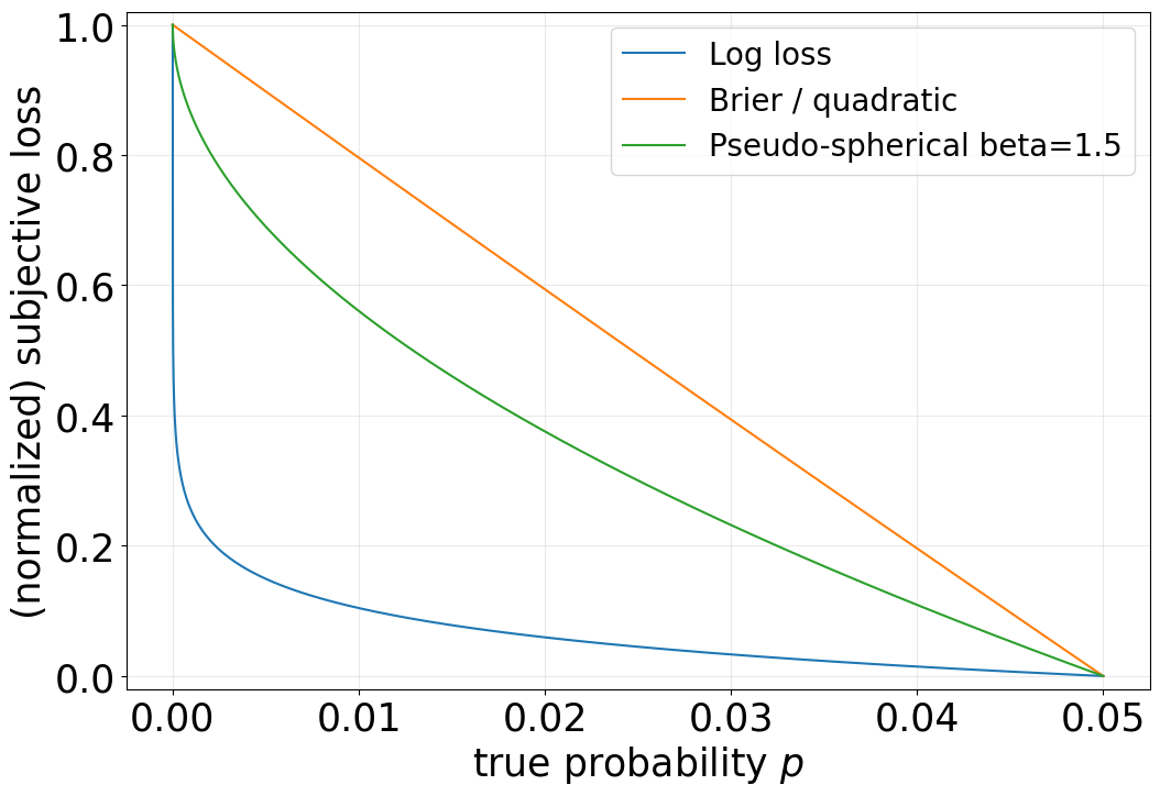
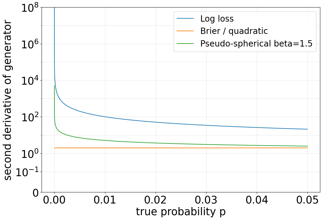
Figure 1: LEFT: Log, Brier, and Pseudo-spherical loss, normalized to a common maximum. RIGHT: Second derivatives of the associated generator function, i.e. \(\nabla^2\phi(p)\)..
The case of log and pseudo-spherical (with \(\beta=1.5\)) rise rapidly as \(p\) approaches zero, affording them sensitivity to probability mass being placed on implausible events, the far left side of the x-axis. The Brier (squared loss) has a slower growth (constant second derivative) and thus less sensitive to mass placed on events that \(p\) regards as implausible.
Objective risk answers the question “how correct is this model?”, whilst subjective risk answers “how realistic is this model?”. Large second derivatives near the boundary are what make a subjective risk sensitive to deviations from reality.
3.5 Summary↩︎
We have presented a novel viewpoint for uncertainty quantification, based on decomposing the subjective risk. This led naturally to many known measures of epistemic and aleatoric uncertainty emerging as decomposition terms, explaining much of the existing literature from a single viewpoint. This provides an interesting point on the additive TU\(=\)AU\(+\)EU view, debated in the literature. From our work, we see AU\(+\)EU is the expected subjective risk with the bias term removed. Those who adopt the additive view are therefore implicitly equating total uncertainty with the ‘de-biased’ expected subjective risk.
4 A Bridge to Statistical Learning Theory↩︎
Classical statistical learning theory (SLT) has provided a rigorous theoretical foundation for supervised learning, enabling the analysis of generalization, sample complexity, and the trade-offs between model capacity and estimation from limited data. It is desirable for uncertainty quantification to have a similar theoretical foundation.
SLT relies on notions such as approximation error, estimation error, and the best-in-class model [10]. These notions are defined with respect to the objective risk, \(R_p(z):=\mathbb{E}_{Y\sim p}[\ell(z,Y)]\). In this section, we introduce corresponding notions induced by subjective risk, \(R_q(z):=\mathbb{E}_{\hat{Y}\sim q}[\ell(z,\hat{Y})]\) and establish basic properties. We consider this as a first step toward a full learning-theoretic framework for uncertainty quantification.
4.1 Defining a Learning Theory nomenclature for Subjective Risk↩︎
Define a hypothesis class \({\mathcal{H}}\subseteq {\mathcal{P}}\), where \({\mathcal{P}}\) is convex, but \({\mathcal{H}}\) is not necessarily convex. As
before, we assume a strictly proper loss with associated regularity/differentiability assumptions. In classical SLT, the expected excess risk of \(q_\theta\in {\mathcal{H}}\) is defined, with the objective risk as
defined throughout the paper, \[\Delta_{obj} := \mathbb{E}_\theta\Big[ R_p(q_\theta) - R_p(p) \Big] = \mathbb{E}_\theta\Big[ B_\phi(p,q_\theta) \Big].\] This quantifies the additional risk (on average w/r uncertainty in
\(\theta\)) that we will have from using a \(q_\theta\), as opposed to the true \(p\). A corresponding notion can be defined for the subjective
risk—the expected excess subjective risk is, \[\Delta_{subj} := \mathbb{E}_\theta\Big[ R_{q_\theta}(p) - R_{q_\theta}(q_\theta) \Big] = \mathbb{E}_\theta \Big[ B_\phi(q_\theta,p)\Big].\] The roles of \(p,q\) have been switched, including the ordering of terms in the expression, since by definition, given our proper loss assumption, \(R_q(q)\leq R_q(p)\), for all \(p,q\). Note however that the expression is still a (non-negative) Bregman divergence.
SLT defines the best-in-class model as the model in \({\mathcal{H}}\) with the smallest expected risk, \[q_{obj}^* := \arg\min_{z\in{\mathcal{H}}} \Big\{ R_p(z) \Big\}.\] Again, we
can define a corresponding subjective version of this as, \[q_{subj}^* := \arg\min_{z\in{\mathcal{H}}} \Big\{ \mathbb{E}_\theta\left[ R_{q_\theta}(z) \right] \Big\}\]
We note that the expected subjective risk is3 the subjective risk of the Bayesian Model Average, i.e., \(\mathbb{E}_\theta \Big [R_{q_\theta}(z) \Big] = R_{\bar{q}}(z)\), which implies \(\bar{q}=\arg\min_{z\in{\mathcal{P}}} \{~ \mathbb{E}_\theta [R_{q_\theta}(z)] ~\}\), but this may not be attainable with non-convex \({\mathcal{H}}\). Therefore, if the BMA \(\bar q \in{\mathcal{H}}\), we have \(q^*_{subj}=\bar{q}\), otherwise \(q^*_{subj}\) is a (sub-optimal) projection to \({\mathcal{H}}\).
Given these definitions, it is interesting to consider when \(q_{\mathrm{obj}}^\ast\) and \(q_{\mathrm{subj}}^\ast\) might coincide—that is, when the argmin of the objective and subjective risks is in fact the same model.
Assume the strictly proper loss admits the Bregman representation in equation 5 , and that the right Bregman projection \(\Pi_{\mathcal{H}}^{R}(r)
:=
\operatorname*{arg\,min}_{z\in\mathcal{H}} B_\phi(r,z)\) exists and is unique for every distribution \(r\) considered below. Then \[q_{\mathrm{obj}}^\ast
=
\Pi_{\mathcal{H}}^{R}(p),
\qquad
q_{\mathrm{subj}}^\ast
=
\Pi_{\mathcal{H}}^{R}(\bar q).\]
Consequently, \(q_{\mathrm{obj}}^\ast=q_{\mathrm{subj}}^\ast\) if and only if \(\Pi_{\mathcal{H}}^{R}(p)
=
\Pi_{\mathcal{H}}^{R}(\bar q).\) In particular, if \(\mathcal{H}=\mathcal{P}\), then \(q_{\mathrm{obj}}^\ast=p\) and \(q_{\mathrm{subj}}^\ast=\bar
q,\) and therefore \(q_{\mathrm{obj}}^\ast=q_{\mathrm{subj}}^\ast\) if and only if \(p=\bar q.\)
Now let \(\bar q_n\) denote the predictive mixture obtained from \(n\) observations. If \(\bar q_n\to p\) and the projection map \(r\mapsto\Pi_{\mathcal{H}}^{R}(r)\) is continuous at \(p\), then \[q_{\mathrm{subj},n}^\ast
=
\Pi_{\mathcal{H}}^{R}(\bar q_n)
\longrightarrow
\Pi_{\mathcal{H}}^{R}(p)
=
q_{\mathrm{obj}}^\ast.\]
Proof. By the proper risk decomposition, \(R_p(z)=B_\phi(p,z)+H_\ell(p),\) where the entropy term does not depend on \(z\). Hence \(q_{\mathrm{obj}}^\ast = \operatorname*{arg\,min}_{z\in\mathcal{H}}B_\phi(p,z) = \Pi_{\mathcal{H}}^{R}(p).\) Similarly, we have \(\mathbb{E}_\theta[R_{q_\theta}(z)] = R_{\bar q}(z) = B_\phi(\bar q,z)+H_\ell(\bar q),\) and therefore \(q_{\mathrm{subj}}^\ast = \operatorname*{arg\,min}_{z\in\mathcal{H}}B_\phi(\bar q,z) = \Pi_{\mathcal{H}}^{R}(\bar q).\) The exact characterization follows immediately. If \(\mathcal{H}=\mathcal{P}\), strict propriety implies that \(B_\phi(r,z)\) is uniquely minimized at \(z=r\). The asymptotic statement follows from the continuity of \(\Pi_{\mathcal{H}}^{R}\). ◻
The proposition distinguishes two notions of optimality. The objective best-in-class model is the element of \(\mathcal{H}\) that best approximates reality \(p\), whereas the subjective best-in-class model best approximates the aggregate predictive belief \(\bar q\). Their coincidence means that internal model beliefs and external reality select the same optimal model within the available hypothesis class. This is desirable when subjective risk is intended to support reliable prediction or action under the true data-generating distribution: minimizing subjective risk then targets the same model as minimizing objective risk.
When \(\mathcal{H}=\mathcal{P}\), coincidence requires the strongest possible form of agreement, namely \(\bar q=p\). For a restricted hypothesis class, however, \(p\) and \(\bar q\) may differ while still having the same projection onto \(\mathcal{H}\). Thus, the result separates disagreement between the distributions themselves from disagreement that actually changes the selected model. The asymptotic statement is particularly useful: if the predictive mixture is consistent and the projection is stable, then the subjective learning target converges to the objective target. In that case, subjective and objective learning are asymptotically aligned.
Conversely, if the two projections differ, the subjective criterion targets a different model from the one preferred under reality. This mismatch is driven by the discrepancy between \(\bar q\) and \(p\), which is measured globally by the bias term \(B_\phi(\bar q,p)\). However, a non-zero bias does not necessarily imply different best-in-class models when \(\mathcal{H}\) is restricted, since two distinct distributions may still have the same projection onto \(\mathcal{H}\).
4.2 Approximation and Estimation from the Subjective Risk↩︎
Classical learning theory decomposes the expected excess (objective) risk as,
\[\Delta_{obj} = \underbrace{ \vrule width 0pt height 0pt depth 1em\relax \mathbb{E}_\theta\Big[ R_p(q_\theta) - R_p(q_{obj}^*) \Big]}_{\textrm{estimation error}} + \underbrace{ \vrule width 0pt height 0pt depth 1em\relax R_p(q_{obj}^*) - R_p(p).}_{\textrm{approximation error}}\] Here, both terms4 are non-negative. The estimation error is the part of the excess risk which can be attributed to insufficient data. We compare models with different parameters \(\theta\), but cannot distinguish their performance on a small dataset—in effect, an instance of the multiple hypothesis testing problem. The estimation error is there because we could not identify the best-in-class model \(q^*_{obj}\in{\mathcal{H}}\). The approximation error is, by contrast, independent of data. It quantifies the notion of model capacity for us—and is non-zero when \({\mathcal{H}}\) is not sufficiently expressive to capture the true \(p\). A well-appreciated tenet of learning theory is the trade off between these terms. As we increase the size of \({\mathcal{H}}\), approximation error decreases monotonically, but estimation error may grow, as it becomes harder to find the best-in-class model with limited data.
We can define a corresponding subjective risk version of this decomposition as, \[\Delta_{subj} = \underbrace{ \vrule width 0pt height 0pt depth 1em\relax \mathbb{E}_\theta\Big[ R_{q_\theta}(p) - R_{q_\theta}(q_{subj}^*) \Big] }_{\textrm{{\boldsymbol{s}ubjective} approximation gap}} + \underbrace{ \vrule width 0pt height 0pt depth 1em\relax \mathbb{E}_\theta\Big[R_{q_\theta}(q_{subj}^*) - R_{q_\theta}({q_\theta}) \Big]}_{\textrm{{\boldsymbol{s}ubjective} estimation error}}\]
We can observe two important differences from the objective risk case. Firstly, the approximation part can be negative—as such we name it a ‘gap’ rather than an ‘error’. Secondly, both terms depend on the model parameters \(\theta\)—this is because \(q_\theta\) is key to the evaluation protocol in the subjective case.
We note that the subjective approximation gap can be written as a difference of two Bregman divergences, \[\mathbb{E}_\theta\Big[ R_{q_\theta}(p) - R_{q_\theta}(q_{subj}^*) \Big] = B_\phi(\bar q , p) - B_\phi(\bar q,q_{subj}^*).\]
If \(q^*_{subj}\) is far from the optimal \(\bar{q}\), then the gap will be negative. On the hand, if \(\bar q=q^*_{subj}\), as in the case of a convex hypothesis class, the subjective approximation gap is non-negative, and in fact equal to the bias term \(B_\phi(\bar{q},p)\).
In contrast to the subjective approximation gap, the subjective estimation error is non-negative, as shown below.
Theorem 2. The subjective estimation error, \(\mathbb{E}_\theta\Big[R_{q_\theta}(q_{subj}^*) - R_{q_\theta}({q_\theta}) \Big]\), is non-negative.
Proof. Using the proper risk decomposition \(R_{q_\theta}(z)=B_\phi(q_\theta,z)+H_\ell(q_\theta)\), it can be written \[\begin{align} \mathbb{E}_\theta\!\left[ R_{q_\theta}(q_{\mathrm{subj}}^*) - R_{q_\theta}(q_\theta) \right] &= \mathbb{E}_\theta\!\left[ B_\phi(q_\theta,q_{\mathrm{subj}}^*) \right] \ge 0. \end{align}\] ◻
4.3 Relation to the Bias–Variance Decomposition↩︎
[32] identified the relationships between bias–variance decompositions and approximation/estimation error, for the case of excess objective risk. We can do the same here, for excess subjective risk. In the objective risk, [32] showed the relationships as, \[\begin{align} \Delta_{obj} &=& \underbrace{ \vrule width 0pt height 0pt depth 1em\relax \mathbb{E}_\theta\Big[ R_p(q_\theta) - R_p(q^*_L) \Big] + R_p(q^*_L) -R_p(q_{obj}^*)}_{\textrm{estimation error}} + \underbrace{ \vrule width 0pt height 0pt depth 1em\relax R_p(q_{obj}^*) - R_p(p)}_{\textrm{approximation error}} \\ &&\underbrace{\phantom{}}_{\textrm{variance}} ~~~ \underbrace{\phantom{}}_{\textrm{bias}} \notag \end{align}\] The corresponding subjective version of this is, \[\begin{align} \Delta_{subj} &=& \underbrace{ \vrule width 0pt height 0pt depth 1em\relax \mathbb{E}_\theta\Big[ R_{q_\theta}(p) - R_{q_\theta}(q_{subj}^*) \Big] }_{\textrm{{\boldsymbol{s}ubjective} approximation gap}} + \underbrace{ \vrule width 0pt height 0pt depth 1em\relax \mathbb{E}_\theta\Big[R_{q_\theta}(q_{subj}^*) - R_{q_\theta}(\bar{q})\Big] + \mathbb{E}_\theta\Big[ R_{q_\theta}(\bar{q}) - R_{q_\theta}(q_\theta) \Big] }_{\textrm{{\boldsymbol{s}ubjective} estimation error}} \notag \\ &&\underbrace{\phantom{}}_{\textrm{bias}} ~~~~ \underbrace{\phantom{}}_{\textrm{variance}} \notag\\ \end{align}\]
From here, we can see an important conclusion.
Theorem 3. For the log proper loss, \(\ell(z,y)=-\ln z(y)\), the variance of the subjective risk (one part of the subjective estimation error) is the mutual information, that is, Gal’s epistemic uncertainty \(I(\hat{Y};\Theta)\).
Proof. Using the proper risk decomposition \(R_{q_\theta}(z)=B_\phi(q_\theta,z)+H_\ell(q_\theta)\), it can be written \[\begin{align} \mathbb{E}_\theta\!\left[ R_{q_\theta}(\bar q) - R_{q_\theta}(q_\theta) \right] &= \mathbb{E}_\theta\!\left[ B_\phi(q_\theta\,,\,\bar q) \right] \ge 0. \end{align}\] Choosing the log loss induces the generalized entropy \(H_\ell(q_\theta)=-\int_{\mathcal{Y}}q_\theta(y)\ln q_\theta(y)\,dy\), whose corresponding Bregman divergence is the (reverse) KL divergence, \[\mathbb{E}_\theta\!\left[ B_\phi(q_\theta\,,\,\bar q) \right] = \mathbb{E}_\theta \left[KL (q_\theta\mid\mid \bar q)\right] = I(\hat{Y};\Theta).\] ◻
The mutual information is only one part of the subjective estimation error—but remaining part is also non-negative, i.e., \(\mathbb{E}_\theta\big[ R_{q_\theta}(q^*_{subj}) - R_{q_\theta}(\bar{q}) \big] = \mathbb{E}_\theta\big[ B_\phi(\bar{q}\,,\,q^*_{subj}) \Big] \geq 0\). The proof of this claim is similar to other results in this section, though we can also see non-negativity via \(\mathbb{E}_\theta\big[ R_{q_\theta}(\bar{q}) \big] = R_{\bar{q}}(\bar{q}) := \inf_{z\in{\mathcal{P}}} R_{\bar{q}}(z)\).
Corollary 1. Mutual information as an epistemic uncertainty measure is a systematic under-estimate of the true subjective estimation error.
Consequently, mutual information captures only one component of subjective estimation error, that represented by posterior disagreement. It ignores the additional error induced by restricting predictions to the hypothesis class. If we take subjective estimation error to be the ‘true’ reducible/epistemic component of the subjective risk, then mutual information should therefore be interpreted as a lower bound on epistemic uncertainty, rather than as its complete characterization.
5 Discussion↩︎
We present a brief discussion of relations to recent work.
5.1 [8]↩︎
The closest work to our own is [8], who identify incoherence in existing discussions across the UQ literature. They state that the community is looking for
“Researchers are looking for concrete notions of a model’s predictive uncertainty and how that uncertainty might or might not change with more data [...] but also related notions of predictive performance and data dispersion. The aleatoric-epistemic view cannot satisfy all these needs: many concepts stand to be defined, while the view fundamentally only has capacity for two concepts.” [8]
To remedy this, they suggest a decision-theoretic perspective. In particular, they use the subjective expected loss of acting Bayes-optimally under a model’s beliefs. They proceed to define epistemic uncertainty as how much this is expected to reduce once future data is observed under Bayesian updating. To account for predictive performance and data dispersion, they separately examine the (objective) risk and entropy of the true \(p\). In summary, they treat uncertainty, external evaluation, and data dispersion as separate objects.
We instead evaluate the subjective risk at the true distribution, \(R_q(p) = \mathbb{E}_{\hat{Y}\sim q}[\ell(p, \hat{Y})]\). We consider it as a quantity that varies with the modelling process, and decompose its expectation. Hence with our approach, the external grounding is built into the risk itself: the bias term accounts for external grounding, while the variance and generalized entropy terms recover the uncertainty quantities.
5.2 [33]↩︎
[33] present a position paper, arguing that epistemic uncertainty estimation methods are fundamentally incomplete. As [34] before them, they discuss uncertainty in the context of statistical learning theory. Critically, they only consider existing theory, i.e., properties of the objective risk. They utilise results from [32] to argue that certain aspects are missing from the community’s understanding of uncertainty. In particular, they consider model bias as a reducible part of epistemic uncertainty that current estimators fail to capture, and conclude on this basis that epistemic estimates are incomplete. We instead view bias as evidence of external grounding rather than an uncertainty component. This distinction is crucial, since a model can have completely certainty, but also be completely wrong. Finally, in their conclusion, they state,
“epistemic uncertainty is generally not well defined and is still a heuristic concept for machine learning models”
We posit that our work has resolved this—providing well-defined terms, with solid links to standard notions from learning theory, and showing how they generate numerous existing proposals as special cases.
5.3 [13]↩︎
Just as in our work, [13], building on [35] also derive uncertainty measures from proper scoring rules and risk decomposition. Their starting point however is what we would refer to as ‘objective’ risk, evaluating expected loss against the true distribution. They consider Bayesian approximations to the risk expressions, substituting various estimates for the unavailable true distribution. Since the approximations can be inserted into either argument of the induced divergence, this generates several candidate measures. By enumerating all combinations of argument orderings, they recover many previously proposed epistemic and aleatoric terms as special cases.
The “all combinations” strategy produces the measures, but does not say which is appropriate for a given modelling scenario, or explain why they behave differently. We instead fix the modelling and evaluation choices first and obtain a single bias–variance–entropy decomposition in which each term has a clear role. The particular measure that appears is then a consequence of the loss geometry rather than a free choice, and disagreements between measures are explained directly by differences in loss curvature (See 3.4).
In the following section, we examine the different epistemic uncertainty measures that arise from varying the arguments and their order.
5.4 The Various Proposals for Epistemic Uncertainty↩︎
The seminal work of [1] introduced the world to mutual information as a measure of epistemic uncertainty. In particular, written in the form \(I(\hat{Y};\Theta) = \mathbb{E}_\theta\left[K(q_\theta\mid\mid\bar{q})\right]\), it has an appealing structure that has led to multiple very similar proposals, from various authors. Here we briefly review these, showing relations to our work.
For simplicity, we restrict discussion to the case of KL divergences on categorical distributions, but the conclusions hold more generally for arbitrary Bregman divergences. As a preliminary step, we remind the reader of the definitions of right and left centroids, defined briefly earlier. The right centroid is, \(q^*_R := \arg\min_{c\in{\mathcal{P}}}\,\,\mathbb{E}_\theta \Big[ K(q_\theta \mid\mid c) \Big] = \mathbb{E}_\theta[q_\theta]\), and the left centroid is, \(q^*_L := \arg\min_{c\in{\mathcal{P}}}\,\,\mathbb{E}_\theta \big[K(c \mid\mid q_\theta)\big] \propto \exp\big( E_\theta \big[ \ln q_\theta \big]\big)\). The left centroid here is a normalized geometric mean, denoted below as \(\mathring{q}\). Note that this is the left centroid only for KL, and for general Bregman divergences \(q^*_L\) is a quasi-arithmetic mean [14]. Given this, we can state the various epistemic uncertainty definitions—see 1.
| Name | KL form | First suggested by |
|---|---|---|
| Mutual Information | \(\E_{\theta} \big[ K (q_\theta \mid\mid \bar{q}) \big]\) | [1] |
| Expected Pairwise KL (EPKL) | \(\E_{\theta}\big[ \E_{\theta'} \left[ K(q_\theta \mid\mid q_{\theta'}) \right]\big]\) | [27] |
| Reverse Mutual Information (RMI) | \(\E_\theta \big[ K(\bar{q}\mid\mid q_\theta) \big]\) | [36] |
| Modified Bregman information | \(\E_\theta \big[ K(q_\theta \mid\mid \mathring{q}) \big]\) | [35] |
| Reverse modified Bregman information | \(\E_\theta\big[ K(\mathring{q}\mid\mid q_\theta) \big]\) | [35] |
These measures follow a common template, with each a variant of the original mutual information form. The template form is \(\mathbb{E}_\theta\big[K(a,b)\big]\), and explores all possible substitutions of arguments \(a,b\) —e.g. with \(a=\mathring{q}\), and \(b=q_\theta\), we get the ‘reverse modified Bregman information’. As mentioned, exactly this, the strategy of ‘all possible combinations’ is adopted by [13]. We note that only two of the terms are ‘standard’ variances in the sense that they are a Jensen gap. These are the first and last rows above: \(\mathbb{E}_\theta[K(q_\theta \mid\mid \bar{q})]\), and \(\mathbb{E}_\theta[K(\mathring{q}\mid\mid q_\theta)]\). As we showed earlier, the mutual information comes from a bias–variance decomposition of the subjective risk. The term \(\mathbb{E}_\theta[K(\mathring{q}\mid\mid q_\theta)]\) is the corresponding variance from the objective risk decomposition. These ‘standard’ Bregman variances are also special in that they are guaranteed to be finite. Reversing the order of arguments, as in RMI and Modified Bregman information, yields non-standard quantities that can be infinite in some cases.
The Expected Pairwise KL, \(\mathbb{E}_{\theta}\big[ \mathbb{E}_{\theta'} \left[ K(q_\theta \mid\mid q_{\theta'}) \right]\big]\), was proposed as an epistemic uncertainty by [27] and later analysed in depth by [37], who found it to have several favourable properties. It is particularly interesting in that it is guaranteed to be finite, and makes intuitive sense as a measure of uncertainty—taking all possible pairwise disagreements. Theorem 4 shows that this is in fact one term in an expansion of the mutual information, and in many cases, the dominant term.
Theorem 4 (Asymmetry decomposition of mutual information). Let \(q_\theta := q(\cdot \mid \theta)\) with \(\theta \sim q(\cdot \mid D)\). Then \[\label{eq:MI95EPKL95RMI46} I(\hat{Y}; \Theta) = \underbrace{ \vrule width 0pt height 0pt depth 0.9em\relax \frac{1}{2}\mathbb{E}_{\theta,\theta'} \Big[ K(q_\theta \mid\mid q_{\theta'})\Big]}_{\textrm{symmetric component}} + \underbrace{ \vrule width 0pt height 0pt depth 0.9em\relax \frac{1}{2} \mathbb{E}_{\theta} \Big[ K(q_\theta \mid\mid \bar{q}) - K(\bar{q} \mid\mid q_\theta) \Big],}_{\textrm{asymmetric component}}\qquad{(1)}\] where \(\bar{q} = \mathbb{E}_\theta[q_\theta]\) and \(\theta, \theta' \overset{\text{i.i.d.}}{\sim} q(\cdot \mid D)\)
Thus, the mutual information contains a symmetric component, and an asymmetric one. The following theorem characterises when the asymmetric term is negligible.
Theorem 5 (EPKL is a 2nd-order approximation of Mutual Information). When the distributions involved are close, i.e.\[q_\theta(y)=q_{\theta'}(y)\bigl(1+\epsilon h(y)\bigr), \qquad \int h(y)q_{\theta'}(y)\,d\nu(y)=0,\] with \(\epsilon\) small, the symmetric component dominates: \[I(\hat{Y};\Theta) ~=~ \frac{1}{2}\mathbb{E}_{\theta,\theta'}\Big[K(q_\theta\mid\mid q_{\theta'})\Big] + O(\epsilon^3).\] This follows because each \(K(q_\theta, q_{\theta'})\) in the symmetric term is of order \(\epsilon^2\), while each asymmetric difference \(K(q_\theta, \bar q) - K(\bar q, q_\theta)\) is of order \(\epsilon^3\). When \(\epsilon\) is small, this implies, \[\mathbb{E}_{\theta,\theta'} \Big[K(q_\theta \mid\mid q_{\theta'})\Big] ~\approx~ 2I(\hat{Y};\Theta).\]
See 9.
The claim is supported by the empirical results in [37]; we replicate selected cases in Figure 2.

6 Conclusion↩︎
We have presented a new view of uncertainty quantification. Rather than treating aleatoric and epistemic uncertainty as primitive quantities that must be independently defined, axiomatized, and defended, we view them as consequences of a more fundamental modelling choice: the risk under which predictive beliefs are evaluated.
Our starting point was Savage’s notion of subjective risk under a strictly proper loss. We adopt this not as a decision-making framework, but as an evaluation functional against reality. Such a loss induces a Bregman divergence geometry, and the corresponding reverse bias–variance decomposition separates the expected subjective risk into systematic bias, variance between predictive distributions, and their generalized entropy. These terms give intuitive meanings to epistemic and aleatoric uncertainty. The epistemic term is the loss-induced Bregman variance of the random predictive distribution, while the aleatoric term is its expected generalized entropy. The validity of this claim is evidenced by exactly recovering numerous previously published proposals as special cases, e.g. [1], [3], [13], [28], [33], [38]. Therefore, these measures should not be understood as competing alternatives, or mutually incompatible definitions: they arise from different losses, geometries, and assumptions.
We proceeded to explore connections with classical statistical learning theory, defining subjective risk analogues of notions such as approximation and estimation error, and their relation to bias–variance decompositions. This yielded various insights, including how existing measures of epistemic uncertainty can fit into a classical learning theoretic framework.
In conclusion, uncertainty measures need not be regarded as primitives requiring independent justification. Instead, they emerge naturally from modelling and evaluation choices through decompositions of subjective risk. Beyond unifying existing uncertainty measures, our perspective shows intriguing connections to statistical learning theory, with analogous definitions of approximation and estimation but for subjective risk. Our hope is that this ‘new view’ will help establish a deeper theoretical foundation for uncertainty quantification.
7 Proofs for 3↩︎
1, the ‘reverse-argument’ BV decomposition, uses the divergence/entropy decomposition of a strictly proper loss to obtain a Bregman divergence, then applies the
right-centroid decomposition from [15] to obtain bias and variance components. We present the full proof here in our notation for completeness.
Proof. of 1. Since \(\ell\) is strictly proper, its generalized entropy \(H_\ell\) is strictly concave, and \(\phi:=-H_\ell\) is strictly convex. Also, as \(\phi\) is differentiable on the relative interior of \({\mathcal{P}}\), this gives the Bregman representation in equation 5 . Hence, \[R_{q_\theta}(p)=\mathbb{E}_{\hat{Y}\sim q_\theta}[\ell(p,\hat{Y})] =B_\phi(q_\theta,p)+H_\ell(q_\theta), \label{eq:thm2-pointwise}\tag{6}\] and assuming expectations are finite,
\[\mathbb{E}_\theta\big[R_{q_\theta}(p)\big] =\mathbb{E}_\theta\big[B_\phi(q_\theta,p)\big]+\mathbb{E}_\theta\big[H_\ell(q_\theta)\big]. \label{eq:thm2-expected}\tag{7}\]
By definition \(q_R^\ast=\arg\min_{z\in{\mathcal{P}}}\mathbb{E}_\theta[B_\phi(q_\theta,z)]\), which is the mixture \(q_R^\ast=\bar q=\mathbb{E}_\theta[q_\theta]\). The Bregman three-point
identity [14], \[B_\phi(q_\theta,p) =B_\phi(q_\theta,\bar q)+B_\phi(\bar q,p)
+\big\langle\nabla\phi(\bar q)-\nabla\phi(p),\,q_\theta-\bar q\big\rangle. \label{eq:thm2-3pt}\tag{8}\] Taking the expectation \(\mathbb{E}_\theta\), the inner-product term vanishes since \(\mathbb{E}_\theta[q_\theta-\bar q]=0\), giving \[\mathbb{E}_\theta\big[B_\phi(q_\theta,p)\big] =\underbrace{B_\phi(\bar q,p)}_{\textrm{bias}}
+\underbrace{\mathbb{E}_\theta\big[B_\phi(q_\theta,\bar q)\big]}_{\textrm{variance}}, \label{eq:thm2-split}\tag{9}\] which is the “reverse-argument” bias–variance decomposition in [15].
Substituting equation 9 into equation 7 yields the stated decomposition, \[\underbrace{\mathbb{E}_\theta\big[\mathbb{E}_{\hat{Y}\sim
q_\theta}[\ell(p,\hat{Y})]\big]} _{\textrm{expected subjective risk}} =\underbrace{B_\phi(\bar q,p)}_{\textrm{bias}} +\underbrace{\mathbb{E}_\theta\big[B_\phi(q_\theta,\bar q)\big]}_{\textrm{variance}}
+\underbrace{\mathbb{E}_\theta\big[H_\ell(q_\theta)\big]}_{\textrm{generalized entropy}}.\] ◻
7.0.0.1 Derivations to support Example 1.
Proof. Let \(\ell(p,\hat{Y})=-\ln p(\hat{Y})\) with \(\hat{Y}\sim q_\theta\), so the pointwise subjective risk of reporting \(p\) under belief \(q_\theta\) is \[R_{q_\theta}(p)=\mathbb{E}_{\hat{Y}\sim q_\theta}\ell(p,\hat{Y}) =-\mathbb{E}_{\hat{Y}\sim q_\theta}\ln p(\hat{Y}) =-\sum_{y\in{\mathcal{Y}}} q_\theta(y)\ln p(y).\] Its generalized entropy is, \[H_\ell(q_\theta):=R_{q_\theta}(q_\theta) =-\sum_{y\in{\mathcal{Y}}} q_\theta(y)\ln q_\theta(y) =H(q_\theta),\] the Shannon entropy of the categorical \(q_\theta\). Hence the generator is \(\phi(q)=-H_\ell(q)=\sum_{y\in{\mathcal{Y}}} q(y)\ln q(y)\), the negative Shannon entropy. The risk decomposes into a generalized entropy and a Bregman divergence (see 5 ): \[R_{q_\theta}(p)=B_\phi(q_\theta,p)+H_\ell( q_\theta ). \label{eq:reverse-cat}\tag{10}\] As \(H_\ell(q)\) is the negative Shannon entropy, the induced Bregman divergence is the reverse KL, \(B_\phi(q_\theta,p)=K(q_\theta\mid\mid p)\). Take expectation \(\mathbb{E}_\theta\) of equation 10 and apply the bias–variance decomposition where \(\bar q:=\mathbb{E}_\theta[q_\theta]\) is the categorical mixture, \[\begin{align} \underbrace{\mathbb{E}_\theta\mathbb{E}_{\hat{Y}\sim q_\theta}[-\ln p(\hat{Y})]} _{\textrm{expected risk}} =& \underbrace{K(\bar q\mid\mid p)}_{\textrm{bias}} + \underbrace{\mathbb{E}_\theta[ K(q_\theta\mid\mid\bar q)]}_{\textrm{variance}} + \underbrace{\mathbb{E}_\theta\big[H(q_\theta)\big]}_{\textrm{generalized entropy}} \end{align}\] The variance term is the mutual information. With \(\hat{Y}\mid\theta\sim q_\theta\) and marginal \(\hat{Y}\sim\bar q\), \[\mathbb{E}_\theta\big[K(q_\theta\mid\mid\bar q)\big] = H(\bar q)-\mathbb{E}_\theta\big[H_\ell(q_\theta)\big] =H(\hat{Y})-H(\hat{Y}\mid\Theta) =I(\hat{Y};\Theta),\] where \(H(\bar q):=-\sum_{y}\bar q(y)\ln\bar q(y)\). Thus the variance is the mutual information \(I(\hat{Y};\Theta)\), understood as epistemic, and the generalized entropy \(\mathbb{E}_\theta[H_\ell(q_\theta)]=H(\hat{Y}\mid\Theta)\), the Shannon conditional entropy, as aleatoric. ◻
7.0.0.2 Derivations to support Example 2.
Proof. Let \(\ell(p,\hat{Y})=-\ln p(\hat{Y})\) with \(\hat{Y}\sim q_\theta\), so the pointwise subjective risk of reporting \(p\) under belief \(q_\theta\) is \[R_{q_\theta}(p)= \mathbb{E}_{\hat{Y}\sim q_\theta} \ell(p,\hat{Y}) = - \mathbb{E}_{\hat{Y}\sim q_\theta}\ln p(\hat{Y}) = - \int_{{\mathcal{Y}}} q_\theta(y) \ln p(y)\, dy.\] Its generalized entropy is, \[H_\ell(q_\theta):=R_{q_\theta}(q_\theta) =-\int_{\mathcal{Y}}q_\theta(y)\ln q_\theta(y)\,dy =\tfrac12\ln(2\pi e\,\sigma_\theta^2),\] the differential entropy of a Gaussian. Thus, \(\phi(q)=-H_\ell(q)=\int_{\mathcal{Y}}q(y)\ln q(y)\,dy\), the negative differential entropy. The risk decomposes into a generalized entropy and a functional Bregman divergence (see 5 ): \[R_{q_\theta}(p) = B_{\phi}(q_\theta,p) + H_\ell(q_\theta) \label{eq:reverse-log}\tag{11}\] as \(H_\ell(q)\) is the negative differential entropy, The induced Bregman divergence is the reverse KL. Take expectation \(\mathbb{E}_\theta\) of equation 11 and apply the bias–variance decomposition where \(\bar q:=\mathbb{E}_\theta[q_\theta]\) is a mixture of distributions, \[\begin{align} \underbrace{\mathbb{E}_\theta\mathbb{E}_{\hat{Y}\sim q_\theta}[-\ln p(\hat{Y})]}_{\textrm{expected risk}} =& \underbrace{K(\bar q \mid\mid p)}_{\textrm{bias}} + \underbrace{\mathbb{E}_\theta[ K(q_\theta\mid\mid \bar q)]}_{\textrm{variance}} + \underbrace{\mathbb{E}_\theta\big[\tfrac12\ln(2\pi e\,\sigma_\theta^2)\big]}_{\textrm{generalized entropy}} \end{align}\] The variance term is the mutual information. With \(\hat{Y}\mid\theta\sim q_\theta\) and marginal \(\hat{Y}\sim\bar q\), \[\mathbb{E}_\theta\big[K(q_\theta\mid\mid\bar q)\big] =\mathbb{E}_\theta \int q_\theta\ln q_\theta-\int\bar q\ln\bar q =H(\bar q)-\mathbb{E}_\theta\big[H_\ell(q_\theta)\big] =H(\hat{Y})-H(\hat{Y}\mid\Theta) =I(\hat{Y};\Theta),\] where \(H(\bar q) := -\int\bar q(y)\ln\bar q(y) dy\). ◻
7.0.0.3 Derivations to support Example 3.
Label-wise UQ [28] treats each label separately as a present/absent event. The indicator of a single label is a Bernoulli variable, so its uncertainty
is fully described by \(\mathrm{Ber}(\mu)\). We show the squared loss example but the idea is more general.
Proof. As in Example 4, the loss is \(\ell(p,\hat{Y})=(\mu_p-\hat{Y})^2\), which induces the same Bregman generator \(\phi(\mu)=\mu^2\) and hence the same divergence \(B_\phi(\mu_\theta,\mu_p)\) between the means. The bias and variance components are therefore identical to Example 2. However, the generalised entropy is the predictive variance, which for the Bernoulli distribution is \[H_\ell(\mu_\theta) := R_{q_\theta}(q_\theta) = \mathbb{E}_{\hat{Y}\sim q_\theta}\big[(\mu_\theta-\hat{Y})^2\big] = \mathbb{E}_{\hat{Y}\sim q_\theta}\big[\hat{Y}^2\big] - \big(\mathbb{E}_{\hat{Y}\sim q_\theta}[\hat{Y}]\big)^2\] Since \(\hat{Y}\sim Ber(\mu_\theta)\) takes values in \(\{0,1\}\), we have \(\hat{Y}^2=\hat{Y}\), so this gives, \[H_\ell(\mu_\theta) = \mu_\theta - \mu_\theta^2 = \mu_\theta \cdot (1-\mu_\theta).\] ◻
8 Further Examples of Bias/Variance for Subjective Risk↩︎
Example 4.
. Variance-based measures [38]. Let \({\mathcal{P}}\) be the class of Gaussians with fixed variance \(\sigma^2=\frac{1}{2}\), and denote the true \(p={\mathcal{N}}(\mu_p,\frac{1}{2})\), and \(q_\theta = {\mathcal{N}}(\mu_\theta,\frac{1}{2})\). Define \(\ell(p,\hat{Y}) = (\mu_p-\hat{Y})^2\). Ignoring affine terms, this induces \(\phi(\mu)=\mu^2\), and 1 becomes, \[\underbrace{ \vrule width 0pt height 0pt depth 1em\relax \mathbb{E}_\theta \Big[ \mathbb{E}_{\hat{Y} \sim q_\theta}\big[ (\mu_p-\hat{Y})^2\big]\Big]}_{\textrm{expected subjective risk}} = \underbrace{ \vrule width 0pt height 0pt depth 1em\relax \Big( \mathbb{E}_\theta[\mu_{\theta} ] - \mu_p \Big)^2}_{\textrm{bias}} ~+~ \underbrace{ \vrule width 0pt height 0pt depth 1em\relax \textcolor{BrightOlive}{ \mathbb{E}_\theta\Big[ ( \mu_{\theta} - \mathbb{E}_\theta[\mu_{\theta} \big] )^2\Big]}}_{\textrm{variance}} ~+ \underbrace{ \vrule width 0pt height 0pt depth 1em\relax \textcolor{red}{ ~\sigma_q^2~} }_{\textrm{generalized entropy}}\] These are the “variance-based” terms studied by many authors for UQ in regression, e.g. [3], [26], [33], [38]. The variance of \(\mu_\theta\), also written as \(Var_\theta(\mathbb{E}_{\hat{Y}\sim q_\theta}[\hat{Y}])\), is again understood as epistemic, and the generalized entropy \(\mathbb{E}_\theta[Var(\hat{Y}\mid\Theta=\theta)]\) as aleatoric. Note, this is constant w/r \(\theta\), and so equal to our assumed \(\sigma^2_q=\tfrac{1}{2}\). The “total uncertainty’ (TU) is their sum, \(Var(\hat{Y})\).
*Furthermore we note that, since we assume \(\sigma_p^2=\sigma_q^2\), this decomposition is exactly equivalent to the classic squared loss bias–variance decomposition [39], with \(\mu_\theta\) as the predictor and \(Y\sim p\) as the true label.*
Proof. Let \(\ell(p,\hat{Y})=(\mu_p-\hat{Y})^2\) with \(\hat{Y}\sim q_\theta\), so the pointwise subjective risk of reporting \(p\) under belief \(q_\theta\) is \[R_{q_\theta}(p)=\mathbb{E}_{\hat{Y}\sim q_\theta}\ell(p,\hat{Y}) =\mathbb{E}_{\hat{Y}\sim q_\theta}\big[(\mu_p-\hat{Y})^2\big].\] Its generalized entropy is, \[H_\ell(q_\theta):=R_{q_\theta}(q_\theta) =\mathbb{E}_{\hat{Y}\sim q_\theta}\big[(\mu_\theta-\hat{Y})^2\big] =\mathbb{E}_{\hat{Y}\sim q_\theta}[\hat{Y}^2]-\big(\mathbb{E}_{\hat{Y}\sim q_\theta}[\hat{Y}]\big)^2 =\sigma_q^2=\tfrac12,\] the predictive variance of \(\hat{Y}\sim q_\theta\), which under the fixed-variance assumption is constant in \(\theta\). Since \(-H_\ell(\mu_\theta)\) equals \(\mu_\theta^2\) up to an affine term, the generator is \(\phi(\mu)=-H_\ell(\mu)=\mu^2\), and the induced Bregman divergence is the squared difference of means, \(B_\phi(\mu_\theta,\mu_p)=(\mu_\theta-\mu_p)^2\). The risk decomposes into a generalized entropy and a Bregman divergence: \[R_{q_\theta}(p)=B_\phi(\mu_\theta,\mu_p)+H_\ell(q_\theta). \label{eq:reverse-var}\tag{12}\] Take expectation \(\mathbb{E}_\theta\) of equation 12 and apply the bias–variance decomposition where \(\bar\mu:=\mathbb{E}_\theta[\mu_\theta]\); the cross term vanishes since \(\mathbb{E}_\theta[\bar\mu-\mu_\theta]=0\), \[\begin{align} \underbrace{\mathbb{E}_\theta\mathbb{E}_{\hat{Y}\sim q_\theta}\big[(\mu_p-\hat{Y})^2\big]} _{\textrm{expected risk}} =& \underbrace{(\bar\mu-\mu_p)^2}_{\textrm{bias}} + \underbrace{\mathbb{E}_\theta\big[(\mu_\theta-\bar\mu)^2\big]}_{\textrm{variance}} + \underbrace{\sigma_q^2.}_{\textrm{generalized entropy}} \end{align}\] ◻
Many ML models have multiple sources of uncertainty—due to uncertainty in training data, initial parameters, procedural training issues, etc. [40] showed how to decompose epistemic uncertainty into procedural and data uncertainty, separating these sources of uncertainty. We can again explain this within our framework. In addition to the bias–variance decomposition, we need the Bregman Law of Total Variance [41], to obtain a finer-grained variance decomposition where appropriate.
Theorem 6 (Bregman Law of Total Variance [41] ). Let \(B_{\phi}\) be a Bregman divergence generated by a strictly convex, differentiable function \(\phi\). Assume a convex class of distributions \({\mathcal{P}}\) over an outcome space \({\mathcal{Y}}\). Let \(q_{\scriptscriptstyle Z}\in{\mathcal{P}}\) be a model induced by a joint* random variable \(Z=(A,B)\). For the reverse-argument Bregman divergence, the variance \(\mathbb{E}_{Z}\big[ B_{\phi}(q_{\scriptscriptstyle Z}, q_R^*) \big]\) can be decomposed by the law of total variance as follows: \[\underbrace{ \vrule width 0pt height 0pt depth 1em\relax \mathbb{E}_{Z} \Big[ B_\phi (q_{\scriptscriptstyle Z}, q_R^*)\Big]}_{\textrm{total variance}} = \underbrace{ \vrule width 0pt height 0pt depth 1em\relax \textcolor{black}{\mathbb{E}_A\Big[ B_{\phi}(q_{\scriptscriptstyle{B\mid A}}^*\,,\,q_R^*) \Big]}}_{\textrm{between-group variance}} + \underbrace{ \vrule width 0pt height 0pt depth 1em\relax \textcolor{black}{\mathbb{E}_A\Big[\mathbb{E}_{B\mid A} \big[B_{\phi}(q_{\scriptscriptstyle Z}\,,\,q_{\scriptscriptstyle{B\mid A}}^*) \big]\Big]}}_{\textrm{within-group variance}}.\] Here \(q_R^* := \arg\min_c \mathbb{E}_{Z} [B_\phi (q_{\scriptscriptstyle Z},c)]\) is the right centroid wrt the joint random variable \(Z\). The conditional right centroid is \(q_{\scriptscriptstyle{B\mid A}}^* := \arg\min_c \mathbb{E}_{B\mid A} [B_\phi (q_{\scriptscriptstyle Z},c)]\). This result is due to [41], with the functional form we use given by [42].*
Proof. The result follows by applying the three-point identity at the conditional centroid and taking iterated expectations, \[B_\phi(q_Z,q_R^\ast) =B_\phi(q_Z,q_{B\mid A}^\ast)+B_\phi(q_{B\mid A}^\ast,q_R^\ast) +\big\langle\nabla\phi(q_{B\mid A}^\ast)-\nabla\phi(q_R^\ast),\,q_Z-q_{B\mid A}^\ast\big\rangle .\] Take \(\mathbb{E}_{B\mid A}\) the inner-product term vanishes since \(\mathbb{E}_{B\mid A}[q_Z-q_{B\mid A}^\ast]=0\), \[\mathbb{E}_{B\mid A}\big[B_\phi(q_Z,q_R^\ast)\big] =B_\phi(q_{B\mid A}^\ast,q_R^\ast) +\mathbb{E}_{B\mid A}\big[B_\phi(q_Z,q_{B\mid A}^\ast)\big].\] Taking \(\mathbb{E}_A\) and using the tower rule \(\mathbb{E}_Z=\mathbb{E}_A\mathbb{E}_{B\mid A}\) gives \[\underbrace{\mathbb{E}_Z\big[B_\phi(q_Z,q_R^\ast)\big]}_{\textrm{total variance}} =\underbrace{\mathbb{E}_A\big[B_\phi(q_{B\mid A}^\ast,q_R^\ast)\big]} _{\textrm{between-group variance}} +\underbrace{\mathbb{E}_A\big[\mathbb{E}_{B\mid A}[B_\phi(q_Z,q_{B\mid A}^\ast)]\big]} _{\textrm{within-group variance}} .\] ◻
If our subjective risk has a joint variable \(Z\), the decomposed variance term from 1 will be \(\mathbb{E}_Z[B_\phi(q_Z\,,\,q^*_R)]\). We can then apply the LTV above, to recover the procedural/data uncertainty split of [40], [43].
Example 5. . Data vs Procedural Uncertainty [33]. Let \({\mathcal{P}}\) be the class of Gaussians with fixed variance \(\sigma^2=\frac{1}{2}\). Define the joint random variable \(Z = (\theta, D)\), where \(\theta\) captures procedural randomness (e.g. weight initialization) and \(D\) captures dataset variations. Denote the true \(p={\mathcal{N}}(\mu_p,\frac{1}{2})\), and \(q_{\scriptscriptstyle Z} = {\mathcal{N}}(\mu_{\scriptscriptstyle Z},\frac{1}{2})\). Define \(\ell(p,\hat{Y}) = (\mu_p-\hat{Y})^2\). Ignoring affine terms, this induces \(\phi(\mu)=\mu^2\), and 1 becomes, \[\underbrace{ \vrule width 0pt height 0pt depth 1em\relax \mathbb{E}_Z \Big[ \mathbb{E}_{\hat{Y} \sim q_Z}\big[ (\mu_p-\hat{Y})^2\big]\Big]}_{\textrm{expected subjective risk}} = \underbrace{ \vrule width 0pt height 0pt depth 1em\relax \Big( \mathbb{E}_{\scriptscriptstyle Z}[\mu_{\scriptscriptstyle Z} ] - \mu_p \Big)^2}_{\textrm{bias}} ~+~ \underbrace{ \vrule width 0pt height 0pt depth 1em\relax \textcolor{BrightOlive}{ \mathbb{E}_{\scriptscriptstyle Z}\Big[\mu_{\scriptscriptstyle Z} - \mathbb{E}_{\scriptscriptstyle Z}[\mu_{\scriptscriptstyle Z} \big] )^2\Big]}}_{\textrm{variance}} ~+ \underbrace{ \vrule width 0pt height 0pt depth 1em\relax \textcolor{red}{ ~\sigma_{q_z}^2~}, }_{\textrm{generalized entropy}}\] where, \[\underbrace{ \vrule width 0pt height 0pt depth 1em\relax \textcolor{BrightOlive}{ \mathbb{E}_{\scriptscriptstyle Z}\Big[\mu_{\scriptscriptstyle Z} - \mathbb{E}_{\scriptscriptstyle Z}[\mu_{\scriptscriptstyle Z} \big] )^2\Big]}}_{\textrm{variance}} ~=~ \underbrace{ \vrule width 0pt height 0pt depth 1em\relax \textcolor{BrightOlive}{ \mathbb{E}_D\Big[ ( \mathbb{E}_{\theta \mid D}[\mu_{\scriptscriptstyle Z}] - \mathbb{E}_{\scriptscriptstyle Z}[\mu_{\scriptscriptstyle Z} \big] )^2\Big]}}_{\textrm{data uncertainty}} ~+~ \underbrace{ \vrule width 0pt height 0pt depth 1em\relax \textcolor{BrightOlive}{ \mathbb{E}_D\Big[\mathbb{E}_{\theta \mid D}\Big[ ( \mu_{\scriptscriptstyle Z} - \mathbb{E}_{\theta \mid D}[\mu_{\scriptscriptstyle Z}] \big] )^2\Big].}}_{\textrm{procedural uncertainty}}\]
Proof. This is Example 4 with the expectation taken wrt a joint variable \(Z=(\theta,D)\), so the squared loss gives \(\phi(\mu)=\mu^2\), bias \((\mathbb{E}_Z[\mu_{\scriptscriptstyle Z}]-\mu_p)^2\), variance \(\mathbb{E}_Z[(\mu_{\scriptscriptstyle Z}-\mathbb{E}_Z[\mu_{\scriptscriptstyle Z}])^2]\), and the constant generalized entropy \(\sigma_{q_{\scriptscriptstyle Z}}^2\). The only new step is to decompose the variance by its source. Applying the Bregman law of total variance (Theorem 6) to \(Z=(A,B)=(D,\theta)\) splits it into a between-group term over datasets and a within-group term over procedural randomness, \[\mathbb{E}_Z\big[(\mu_{\scriptscriptstyle Z}-\mathbb{E}_Z[\mu_{\scriptscriptstyle Z}])^2\big] =\underbrace{\mathbb{E}_D\big[(\mathbb{E}_{\theta\mid D}[\mu_{\scriptscriptstyle Z}]-\mathbb{E}_Z[\mu_{\scriptscriptstyle Z}])^2\big]} _{\textrm{data}} +\underbrace{\mathbb{E}_D\big[\mathbb{E}_{\theta\mid D}[(\mu_{\scriptscriptstyle Z}-\mathbb{E}_{\theta\mid D}[\mu_{\scriptscriptstyle Z}])^2]\big]} _{\textrm{procedural}},\] recovering the data/procedural decomposition discussed in [40], [43], and [33]. ◻
Example 6. . Deep Ensembles. [3] propose an axiomatic framework, with Deep Ensembles [30] as an exemplar. Assume the same setting as Example 4, but now with unknown variance* and a finite set of \(m\) models: each \(\theta_i\) induces \(q_{\theta_i}={\mathcal{N}}(\mu_i,\sigma_i^2)\), so the expectation over \(\theta\) becomes a finite average \(\tfrac{1}{m}\sum_{i=1}^m\). \[\underbrace{ \vrule width 0pt height 0pt depth 1.8em\relax \frac{1}{m}\sum_{i=1}^m \Bigg[ \mathbb{E}_{\hat{Y} \sim q_{\theta_i}}\left[ (\mu_p-\hat{Y})^2\right]\Bigg] }_{\textrm{expected subjective risk}} = \underbrace{ \vrule width 0pt height 0pt depth 1.8em\relax \left( \frac{1}{m}\sum_{i=1}^m \mu_i - \mu_p \right)^2}_{\textrm{bias}} + \underbrace{ \vrule width 0pt height 0pt depth 1.8em\relax \textcolor{BrightOlive}{ \vrule width 0pt height 0pt depth 1em\relax \frac{1}{m}\sum_{i=1}^m\mu_i^2 - \left(\frac{1}{m}\sum_{i=1}^m\mu_i\right)^2 }}_{\textrm{variance}} + \underbrace{ \vrule width 0pt height 0pt depth 1.8em\relax \textcolor{red}{ \frac{1}{m}\sum_{i=1}^m\sigma_i^2}}_{\substack{\textrm{generalized}\\ \textrm{entropy}}} \notag\] The epistemic/aleatoric terms are exactly those derived in [3].*
Proof. This is Example 4 with the posterior over \(\theta\) replaced by the distribution over a finite set of \(m\) members, so every expectation \(\mathbb{E}_\theta\) becomes the average \(\tfrac 1m\sum_{i=1}^m\) and each member contributes \(q_{\theta_i}=\mathcal{N}(\mu_i,\sigma_i^2)\). Allowing \(\sigma_i^2\) to vary across members is the only difference from Example 4. ◻
9 Proofs for 5↩︎
We prove the relation between mutual information and EPKL [37].
Proof. of 4. Multiplying the expression by \(2\) and rearranging gives \[\begin{align} 2 \cdot I (\hat{Y}; \Theta) &= \mathbb{E}_{\theta,\theta'} K(q_\theta \mid\mid q_{\theta'}) + \mathbb{E}_{\theta} \Big[ K(q_\theta \mid\mid \bar q) - K(\bar q \mid\mid q_\theta) \Big]\notag\\ I (\hat{Y}; \Theta) &= \mathbb{E}_{\theta,\theta'} K(q_\theta \mid\mid q_{\theta'}) - \mathbb{E}_{\theta} K(\bar q \mid\mid q_\theta)\notag \end{align}\] Rearranging this final equation yields exactly [36], \(RMI = EPKL - MI\), which completes the proof. ◻
Proof. of [thm:smallDisagreementExpansion]. Let \((\mathcal{Y},\mathcal{A},\lambda)\) be a measure space, and let \(q_0\) be a strictly positive probability density with respect to \(\lambda\). For each \(\theta\), suppose \[q_\theta(y)=q_{\theta'}(y)\bigl(1+\epsilon h(y)\bigr), \qquad \int h(y)q_{\theta'}(y)\,d\nu(y)=0,\] where the perturbations satisfy \(\|r_\theta\|_\infty \leq M \quad\text{almost surely},\) for \(|\epsilon|M<1\), and \[\int q_0(y)r_\theta(y)\,d\lambda(y)=0 \quad\text{for every }\theta .\] Assume also that \(\mathbb{E}_\theta[r_\theta(y)] = 0\), for \(q_0\text{-almost every }y\). Then, \(\bar q(y):=\mathbb{E}_\theta[q_\theta(y)] = q_0(y)\). Let \(\theta,\theta'\) be independent draws from the posterior over parameters, and define \(\mathrm{EPKL}_\epsilon := \mathbb{E}_{\theta,\theta'} K(q_\theta\mid\mid q_{\theta'})\) and \(A_\epsilon := \mathbb{E}_\theta \left[ K(q_\theta\mid\mid \bar q) - K(\bar q\mid\mid q_\theta) \right]\). Then, as \(\epsilon\to 0\), \[\label{eq:epkl95second95order} \mathrm{EPKL}_\epsilon = \epsilon^2 \mathbb{E}_\theta \left[ \int q_0(y)r_\theta(y)^2\,d\lambda(y) \right] + O(\epsilon^3),\tag{13}\] whereas \[\label{eq:asymmetry95third95order} A_\epsilon = \frac{\epsilon^3}{6} \mathbb{E}_\theta \left[ \int q_0(y)r_\theta(y)^3\,d\lambda(y) \right] + O(\epsilon^4).\tag{14}\] Consequently, if \[V_2 := \mathbb{E}_\theta \left[ \int q_0(y)r_\theta(y)^2\,d\lambda(y) \right] >0,\] then \[\frac{A_\epsilon}{\mathrm{EPKL}_\epsilon} = O(\epsilon).\] Therefore the asymmetry correction is negligible relative to the expected pairwise KL in the small-disagreement regime. In particular, since \[I(\hat{Y};\Theta) = \frac{1}{2} \mathrm{EPKL}_\epsilon + \frac{1}{2} A_\epsilon,\] we have \[\label{eq:mi95epkl95approx} I(\hat{Y};\Theta) = \frac{1}{2} \mathbb{E}_{\theta,\theta'} K(q_\theta\mid\mid q_{\theta'}) + O(\epsilon^3).\tag{15}\] Equivalently, \[\mathbb{E}_{\theta,\theta'} K(q_\theta\mid\mid q_{\theta'}) = 2I(\hat{Y};\Theta) + O(\epsilon^3).\] ◻
References↩︎
Convexity (or lack thereof) here has a relevant and natural philosophical interpretation: given two distributions \(P_1, P_2 \in \mathcal{P}\), then any convex combination \(\lambda P_1 + (1-\lambda)P_2\), with \(\lambda \in [0,1]\), may also be regarded as ‘plausible’. Thus, \({\mathcal{H}}\) may or may not be closed under mixtures of ‘plausible’ distributions.↩︎
Depending on loss geometry, as we will see later.↩︎
Trivially, \(\mathbb{E}_\theta \left[ R_{q_\theta}(z) \right] = \mathbb{E}_\theta \left[\int_{{\mathcal{Y}}} \ell(z,y) q_\theta(y) \,d\nu(y) \right] = \int_{{\mathcal{Y}}} \ell(z,y) \bar q(y) \,d\nu(y) := R_{\bar q}(z)\).↩︎
We follow the convention of [31] in that the first term in the decomposition is called ‘estimation error’ as opposed to ‘expected estimation error’.↩︎