Can We Trust Item Response Theory
for AI Evaluation?
July 16, 2026
Abstract
AI benchmarks increasingly leverage item-level statistical models, particularly item response theory (IRT), to estimate model capabilities, rank systems, select informative examples, and diagnose benchmark quality. However, AI benchmark data often departs from the data regime of human testing, for which standard IRT estimation tools were originally developed: benchmarks typically involve fewer evaluated models, far more items, and capability distributions that may be skewed, clustered, or multimodal. We examine how these regime mismatches challenge the reliability of IRT modeling for AI evaluation. Using item parameters and capability distributions derived from six widely used LLM benchmarks, we simulate response matrices under three common IRT models and compare four estimation tools used in recent benchmark studies: marginal maximum likelihood, Markov chain Monte Carlo, variational inference, and a neural pseudo-Siamese estimator. Across 18,000 simulation conditions, we systematically evaluate computational feasibility, scalability, and the reliability of IRT inferences about model rankings, predicted performance, and item characteristics. Results show that classical estimators can become infeasible in large benchmark settings, whereas scalable estimators can produce unreliable item-level and ranking inferences with small or nonnormally distributed model sets. This study identifies when latent trait models reliably support or risk distorting AI benchmarking claims, and what sample sizes and diagnostics are needed for trustworthy use.
1 Introduction↩︎
AI benchmarks have become the primary instrument for evaluating model capabilities, comparing AI systems, and informing deployment decisions. Yet the dominant practice of relying on aggregate metrics such as mean accuracy is deceptively simple: it reduces a rich response matrix to a single number, treating all items as equally informative regardless of their difficulty or discriminative power [1], [2]. This simplification dilutes informative signals in evaluation data, renders model rankings sensitive to benchmark composition, and hinders the accumulation of comparable findings across evaluation efforts, reflecting a deep tension between validity, reliability, and efficiency [3], [4].
This tension naturally directs attention to psychometrics, the discipline devoted to the science of human testing and assessment, for well-established measurement tools. Item response theory (IRT), the most widely adopted statistical framework, offers a principled alternative. Instead of treating each item equally, IRT jointly estimates parameters of item characteristics and examinee ability on a shared latent scale, enabling in-depth diagnosis of item quality, efficient testing through adaptive item selection, and cross-benchmark comparison of ability estimates [5]. Motivated by these advantages, a growing body of work has adopted IRT for AI evaluation, applying it to produce finer-grained model and item diagnostics (e.g., [6], [7]) and enable more efficient evaluation strategies, such as adaptive AI testing (e.g., [8], [9]) and benchmark compression (e.g., [10]).
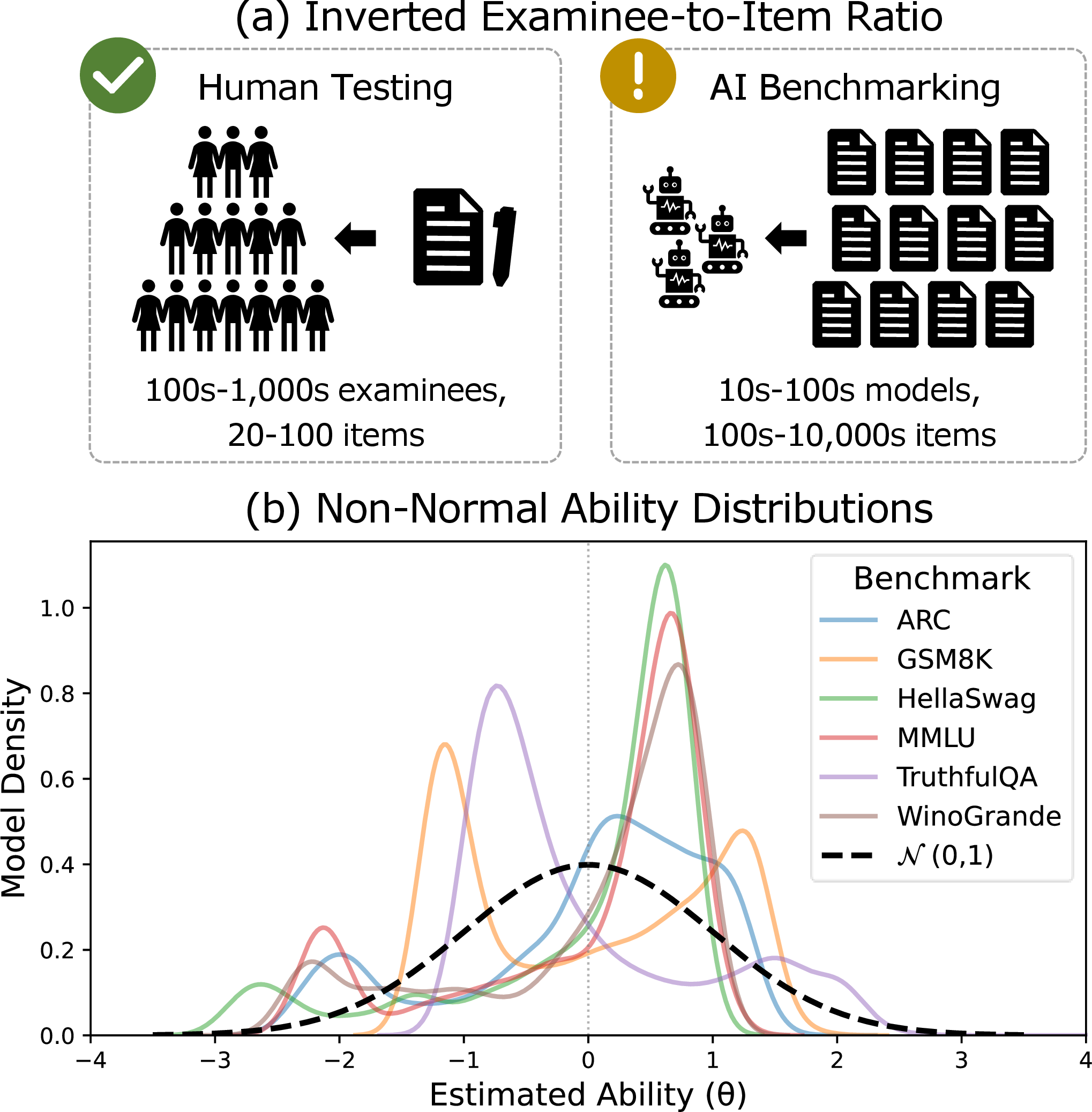
Nevertheless, the adoption has outpaced validation. A crucial concern is that AI benchmark data fundamentally depart from the human testing regime for which IRT estimation methods were developed and validated. As illustrated in Fig. 1, the number of evaluated models is typically small (fewer than 100) while the number of items can reach tens of thousands – an inversion of the typical psychometric setting, where hundreds to thousands of examinees respond to tests of 20-100 items [11]. Furthermore, the model capability distributions are frequently non-normal, exhibiting multimodality or skewness that conflicts with the normality assumptions underlying standard estimation procedures [12], [13]. These departures matter because IRT’s statistical validity depends directly on the sample-to-parameter ratio and the match between the assumed distribution and the true one; dual violations risk producing systematically biased estimates of both item characteristics and model capabilities.
Existing studies that apply IRT do not focus on verifying whether the chosen IRT models and estimation methods produce reliable estimates under this regime mismatch, leaving critical questions unanswered. It remains unknown how small model populations, non-normal ability distributions, and long benchmarks affect parameter recovery and downstream inferences such as model rankings and item-level diagnostics. Practical guidance for conducting such studies is equally lacking: for instance, when constructing an item-level benchmark repository (e.g., [14]), how many evaluated models will be sufficient to fit a given IRT model reliably?
To the best of our knowledge, no prior work has systematically addressed these questions. This paper fills this gap through three contributions:
A literature review surveying 19 studies that apply IRT to AI benchmarking, characterizing the current landscape of IRT usage and empirically identifying the range of application conditions that inform the design of our simulation study (Sec. 3).
A simulation study calibrated to representative AI evaluation data regimes, systematically evaluating computational feasibility, parameter recovery, and downstream inference validity across six benchmarks, three IRT models, four estimators, and five sample sizes (Secs. 4 & 5).
Practical guide based on the findings, including recommendations on minimum sample sizes, IRT model selection, and estimation methods, clarifying when IRT reliably supports AI benchmarking claims and when it risks distorting them (Sec. 6).
Sec. 2 provides the necessary background on IRT and simulation methodology, and Sec. 7 concludes.
2 Background↩︎
2.1 Item response theory↩︎
The limitations of aggregate metrics for AI evaluation naturally motivate the adoption of item response theory (IRT), a family of statistical models from psychometrics. Unlike simpler measurement methods such as classical test theory [15], [16], it does not assume that each item is equally difficult, but separately quantifies item characteristics and examinee ability on a common latent scale [5], [17].
Specifically, IRT models the probability of the correct response to an item as a function of a latent ability parameter \(\theta\) and one or more item-level parameters capturing item characteristics [18]. Its simplest form, the one-parameter logistic model (1PL, also known as the Rasch model [19]), characterizes each item solely by its difficulty \(b\): \(p(y\!=\!1|\theta, b)=\sigma(\theta\!-\!b)\), where \(y\!\in\!\{0, 1\}\) denotes the response correctness and \(\sigma(\cdot)\) is the sigmoid function. The two-parameter logistic model (2PL) introduces a discrimination parameter \(a\), allowing items to differ in how effectively they distinguish between high- and low-ability examinees: \(p(y\!=\!1|\theta, a,b)=\sigma(a(\theta\!-\!b))\). The three-parameter logistic model (3PL) further adds a guessing parameter \(c\), representing the probability that an extremely low-ability examinee responds correctly: \(p(y\!=\!1|\theta, a,b)=c\!+\!(1\!-\!c)\sigma(a(\theta\!-\!b))\) [20]. Extensions such as the 4PL [21] and the graded response model [22] incorporate additional parameters into the response function.
In practice, IRT models are calibrated using observed response data from settings such as educational testing and AI benchmarking. Given a response matrix \(Y \in \{0,1\}^{N\!\times\!J}\) where each entry \(y_{i,j}\) records whether examinee \(i\) answered item \(j\) correctly, an IRT model is fit to jointly estimate \(\theta_i\) for each examinee and the item parameter(s) \(\boldsymbol{\zeta}_j=\{b_j, ...\}\), for each item. Standard estimators include marginal maximum likelihood via EM (MML-EM [23]), Markov chain Monte Carlo (MCMC [24], [25]), and variational inference (VI [26]), which we elaborate on in Sec. 3. These estimates enable downstream analyses such as flagging problematic items, constructing shorter yet equally diagnostic tests, and producing examinee rankings on a common scale with associated uncertainty.
Despite these benefits, we highlight that key assumptions underlying IRT fundamentally conflict with the data regime of AI evaluation, which calls into question the trustworthiness of IRT-based AI benchmark analysis. Standard IRT estimators require large examinee samples (typically \(N\!\geq\)500 for 2PL and \(N\!\geq\)1,000 for 3PL [11]) for estimation accuracy, and most further impose normal ability distribution assumptions, either as an explicit population assumption (MML-EM) or through prior specification (Bayesian and VI). AI benchmarking data often violate both assumptions: the number of examinees (models) is typically small, while the number of items often reaches tens of thousands [27]; and model ability distributions could be bimodal or skewed, bearing little resemblance to the assumed normal distributions [12], [13]. The evaluated model population is also rapidly evolving, further questioning the assumption of distributional norms for model capability.
2.2 Simulation studies: evaluating the evaluator↩︎
Simulation studies, also known as Monte Carlo studies or parameter recovery studies, are the standard methodology for evaluating the performance of statistical methods under controlled conditions [28]. The general procedure follows a well-established workflow:
specify true values for parameters that are ordinarily unobservable,
generate simulated response data from these known parameters,
fit the model of interest to the simulated data, and
compare the estimated parameters against the data-generating ground truth,
which has been formalized as the ADEMP framework: Aims of the study, Data generation mechanisms, Estimated parameters, Methods being evaluated, and Performance measures, which provides coherent guidance for planning and reporting simulation studies [29]. The methodology enables direct manipulation of simulation conditions and measurement of estimation quality against known ground truth, isolating the effects of specific conditions on method performance.
A simulation study for IRT thus serves as a means of evaluating the evaluator itself: by systematically varying simulation conditions such as the number of evaluated models, the distribution of model capabilities, the size of AI benchmarks, and the choice of IRT models, we can gain direct evidence on whether the resulting estimates (i.e., model capabilities and item parameters) genuinely reflect targeted latent traits. In psychometrics, a substantial body of simulation research has investigated the conditions under which IRT estimates for human testing are trustworthy (e.g., [30], [31]), establishing the practical guidelines and assumptions outlined in Sec. 2.1. For example, recommended minimum sample sizes are 250–500 for 1PL and 2PL [11], [32], [33], and 1,000–3,000 for 3PL [11]. These studies also document how assumption violations, such as non-normal ability distributions or short test lengths, degrade estimation quality (e.g. [34]–[36]). However, these guidelines were developed under the human testing conditions described above. The AI evaluation setting departs from all those conditions simultaneously, yet no prior work has conducted such simulations in this context. This paper thus addresses this gap with a comprehensive simulation study calibrated to representative AI evaluation conditions observed in our literature review.
3 Item response theory for AI evaluation↩︎
Taking the simple average score on a benchmark ignores that not all benchmark items are equally informative [1]. Items with poor discriminative power, such as those on which models perform similarly regardless of overall capability, do not contribute capability-relevant signal [37]. As models rapidly evolve and more items become trivially easy, this becomes increasingly common [38], [39]. Worse, some items may capture shortcuts such as spurious correlations or format heuristics rather than the intended capability, jeopardizing the validity of score interpretations. Without principled methods to identify and down-weight such uninformative items, they contribute equally to aggregate scores alongside more diagnostic items. Furthermore, benchmark-specific average score lacks mechanisms to place models evaluated on different benchmarks on a common scale [40], hindering the accumulation of comparable findings across evaluation efforts.
IRT emerged as a viable approach to address these AI benchmarking challenges. As a survey of current IRT applications to address these limitations, we conducted a scoping review. We searched arXiv using keywords related to item response theory (IRT), AI evaluation, and AI benchmarking, covering publications from 2016 to 2026. Two authors independently screened the results against predefined inclusion criteria: studies must apply IRT or related item-factor models to model evaluation in AI, ML, or NLP contexts; studies that merely cite IRT without applying it were excluded. This process identified 19 studies.
Across these studies, IRT-style probablistic models have been used to support (1) latent capability scoring that accounts for item difficulty or discrimination in place of simple aggregate scores [1], [6], [41], [42]; (2) item and benchmark analysis, including the identification of difficult, informative, saturated or weakly discriminating examples [1], [7], [12], [43]–[45]; and (3) efficient evaluation through smaller item subsets, adaptive item administration or generation, and prediction of performance on unseen items or tasks, reducing the need to run every model on full benchmarks [3], [6], [8]–[10], [46]–[48]. IRT model specifications ranged from standard binary 1PL, 2PL, 3PL and 4PL, with either unidimensional or multidimensional latent ability spaces, to adaptations for data formats including pairwise comparisons (e.g., [49]), continuous scores (e.g., [47]), response-length information [50], and item text features (e.g., [48]). The unidimensional 2PL with item-specific difficulty and discrimination parameters was the most commonly adopted model.
Most of these studies fitted IRT models to binary response matrices, in which rows represent evaluated models and columns represent benchmark examples, or items. However, the row and column dimensions differed substantially from typical human-testing contexts and varied substantially across studies. Many included tens to low hundreds of evaluated models, including cases below 50, with analyses based on OpenLLM Leaderboard [51] as the main exception, where model counts exceeded 5,000. Benchmark length, by contrast, ranged from a few hundred to more than 80,000 examples. Estimation methods were also heterogeneous, including marginal or full-information maximum likelihood via the EM algorithm [6], [9], MCMC [3], [7], [47], variational inference [1], [8], [10], [52], and neural-network representations of IRT models fit with gradient-based optimization [8], [12].
This variation motivates a methodological study that examines how evaluated model count, benchmark length, capability distribution, IRT model specification and estimation method affect the reliability of item- and model-level inferences used to construct and interpret AI benchmark claims.
4 Simulation design↩︎
The simulation aims to examine when existing IRT estimation approaches provide reliable item- and model-level inferences under data regimes observed in AI evaluation. The data conditions, estimation methods, and evaluation metrics were chosen to reflect common practices in recent applications of IRT to AI benchmark analysis.
4.1 Data generation↩︎
4.1.0.1 IRT model, sample size, and benchmark.
For IRT model, we focus on unidimensional 1PL, 2PL, and 3PL as the most commonly adopted specifications in the reviewed studies.
Sample sizes, i.e., the number of evaluated model, were chosen from the empirical range observed across the studies in Sec. 3: \(N\!=\!30\), similar to sample sizes found in in [9], [10], [12]; \(N\!=\!100\), similar to [3], [8], [10], [52]; \(N\!=\!180\), similar to [1], [9]; \(N\!=\!400\), similar to [10]; and \(N\!=\!1000\), as a reference condition closer to sample-size recommendations for 3PL estimation in human testing.
Benchmark conditions were based on the OpenLLM Leaderboard v1 benchmarks analyzed in [3], [6], [10]. The leaderboard aggregates results from over 6,000 community-contributed models across six benchmark datasets: ARC-Challenge [53], HellaSwag [54], MMLU [55], TruthfulQA [56], WinoGrande [57], and GSM8K [58], spanning tasks from commonsense reasoning to mathematical problem solving, with benchmark lengths ranging from approximately 800 to 15,000 items. In total, this yields \(3\!\times\!5\!\times\!6\!=\!\boldsymbol{90}\) unique simulation conditions.
4.1.0.2 True parameters and response matrices.
The true item parameters and model capability distributions were derived from the preprocessed OpenLLM response matrices used in [6], which contain binary responses from over 6,000 models across the six benchmarks. Following their preprocessing, models with the lowest 0.1% of scores were removed to reduce noise, and items with standard deviations below 1% or mean accuracies above 95% were excluded as uninformative or nearly saturated. The retained matrices dimensions (\(N\) models \(\times J\) items) were as following: \(5,222\!\times\!644\) for TruthfulQA, \(5,221\!\times\!844\) for ARC-Challenge, \(6,550\!\times\!1,045\) for WinoGrande, \(6,068\!\times\!1,306\) for GSM8K, \(5,221\!\times\! 5,711\) for HellaSwag, and \(5,219\!\times\!12,508\) for MMLU.
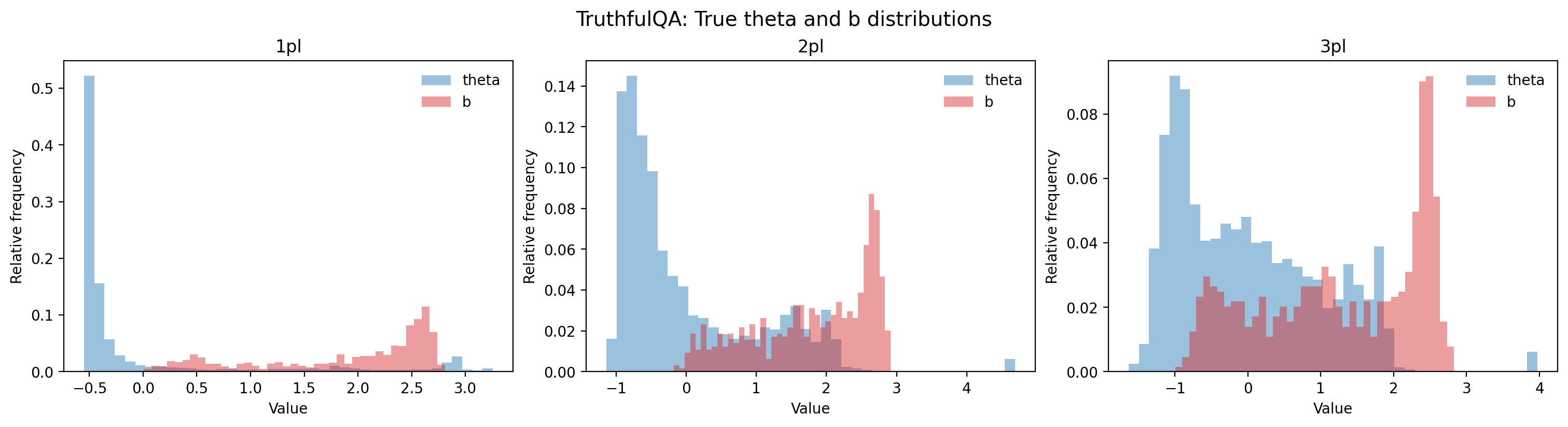
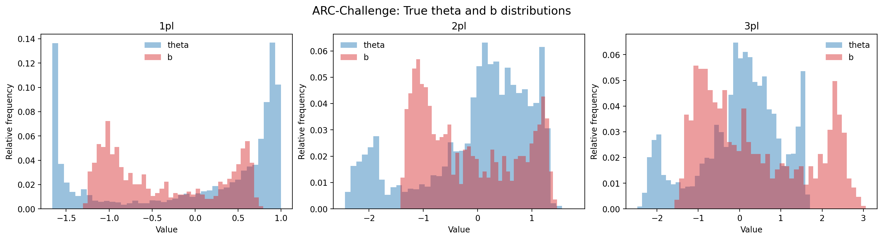
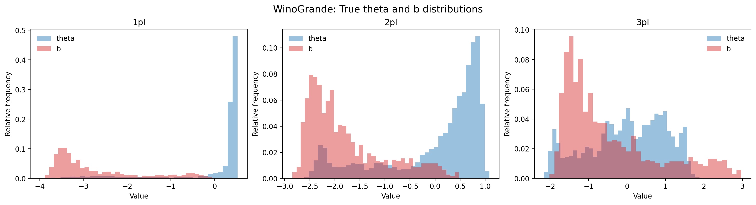
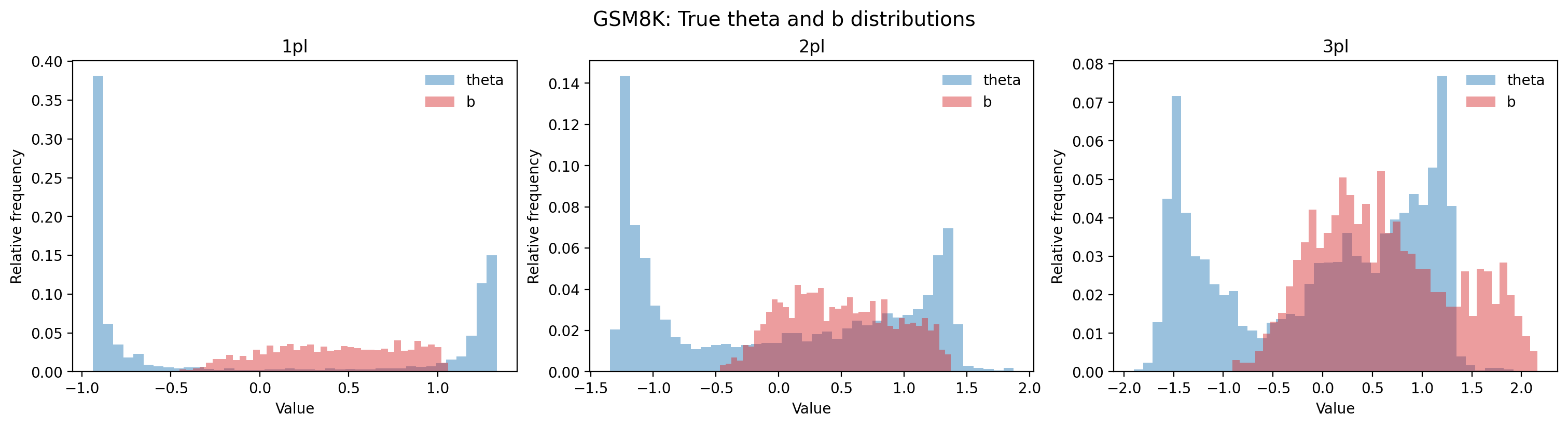
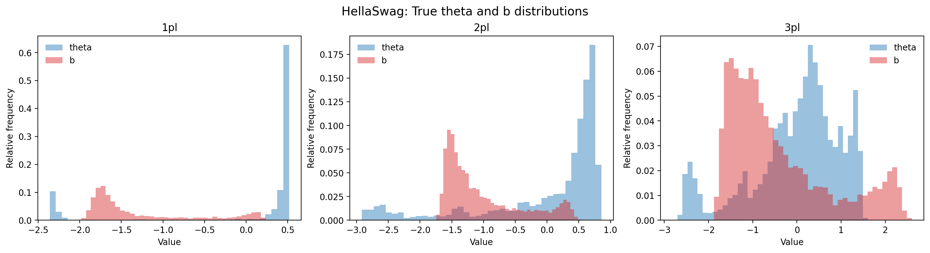
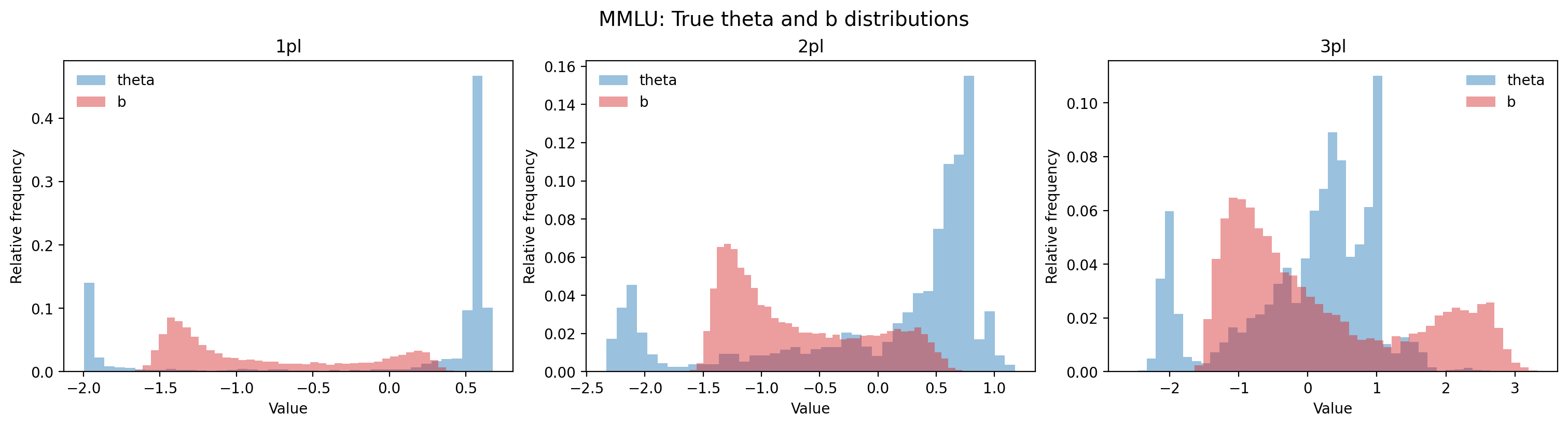
For each benchmark, we fit the 1PL, 2PL and 3PL models to the empirical response matrix using variational inference, which allowed us to estimate parameters for all items and models in each benchmark jointly while remaining computationally tractable. The resulting item parameter estimates were treated as the true item parameters in the simulation. Figs. 6–11 in App. 9 present the distributions of the estimated model capabilities and true difficulty parameters for each benchmark, illustrating the preserved distributional features such as skewness, clustering, and multimodality.
For each of the 90 conditions, we generated 50 replications. In each replication, \(N\) true capability values were sampled from the empirical distribution of the estimated abilities for the corresponding condition. The sampled ability values and the item parameters were then used to generate a full binary response matrix, which was used as the input data for IRT estimation.
4.2 Estimation↩︎
We evaluated four IRT estimatiors spanning the major paradigms used in recent IRT-based AI evaluation studies (Sec. 3): MML-EM, MCMC, VI, and PSN. Full technical details, including formulations, prior specifications, and implementation settings, are provided in App 8.
MML-EM estimates item parameters by maximizing the marginal likelihood, integrating out latent abilities under an assumed population distribution, typically standard normal. It is the conventional approach in psychometrics, implemented
here via the Metropolis-Hastings Robbins-Monro algorithm, a stochastic variant of EM, in the mirt R package [59] for improved computational
efficiency. MML assumes a fixed, known ability distribution and its statistical consistency guarantees require \(N \to \infty\) with \(J\) fixed, which is inverted in AI benchmarking.
MCMC performs full Bayesian inference, sampling from the joint posterior over item parameters and examinee abilities. We used Stan’s Hamiltonian Monte Carlo via the brms R package [60]. MCMC iteratively samples parameters from the posterior distribution with computational demand scaling in \(N\), \(J\) and chain length.
VI approximates the Bayesian posterior with a factorized variational distribution, optimized via KL divergence minimization. We used the implementation in the Python package, py-irt [61]. VI is computationally attractive for larger response matrices as it replaces the posterior sampling with gradient-based optimization. However, it inherits the prior assumptions of the Bayesian model
and adds approximation error from the chosen variational family. PSN is a neural-network estimator that learns ability and item parameter embeddings, which are passed through an IRT response function to predict binary responses, trained
with gradient-based optimization [12]. Unlike the other estimators, PSN does not impose a parametric distribution on abilities, but it does not directly provide
uncertainty quantification or consistency guarantees for its estimates.
4.3 Evaluation metrics↩︎
The evaluation covers computational feasibility and the three IRT use cases identified in Sec. 3: latent capability scoring, item analysis, and efficient benchmarking, resulting in four corresponding subsections in Sec. 5.
4.3.0.1 Computational feasibility.
Computational feasibility was summarized by failure rate (the proportion of replications that failed to produce parameter estimates) and per-replication runtime for completed runs. For MML-EM, failures also included non-convergence when the algorithm terminated without satisfying the convergence criterion after 2,000 cycles.
4.3.0.2 Latent capability scoring.
For model capability, ranking recovery was evaluated using Kendall’s rank (\(\tau\)) correlation between true and estimated capability values. Additionally, we measured aggregate score error: the absolute difference between expected full-benchmark scores under true and estimated parameters, \(\left|\frac{1}{J}\sum_{j=1}^{J}\pi_{ij}-\frac{1}{J}\sum_{j=1}^{J}\hat{\pi}_{ij}\right|\), averaged across models, where \(\pi_{ij}=P(Y_{ij}=1\mid \theta_i,\boldsymbol{\zeta}_j)\) and \(\hat{\pi}_{ij}=P(Y_{ij}=1\mid \hat{\theta}_i,\hat{\boldsymbol{\zeta}}_j)\) denote model \(i\)’s correct response probability on item \(j\) based on true and estimated parameters, respectively.
4.3.0.3 Item analysis.
Recovery of item-level properties was evaluated using Pearson correlations between true and estimated item parameters, including difficulty recovery and discrimination recovery (2/3PL), and the average absolute error in estimated guessing probability (3PL), i.e., \(\frac{1}{J}\sum_{j=1}^{J}|\hat{c}_j-c_j|\). Similar to aggregate score error, we measured mean item error as absolute deviation between item-level correct response probabilities computed from estimated and true parameters, \(\left|\frac{1}{N}\sum_{i=1}^{N}\pi_{ij}-\frac{1}{N}\sum_{i=1}^{N}\hat{\pi}_{ij}\right|\), averaged across items.
4.3.0.4 Efficient benchmarking.
To assess IRT’s effectiveness in AI benchmark compression, Fisher information \(\mathcal{F}\) [5] was computed for each item \(j\) given each model’s estimated capability value \(\hat{\theta}_i\): \[\hat{\mathcal{F}}_{j}(\hat{\theta}_i) = \hat{a}_j^2 \cdot \frac{(\hat{\pi}_{ij}-\hat{c}_j)^2}{(1-\hat{c}_j)^2} \cdot \frac{1-\hat{\pi}_{ij}}{\hat{\pi}_{ij}} .\] For 1PL and 2PL, \(\hat{c}_j=0\), and for 1PL, \(\hat{a}_j= 1\). The top 10% of items with tha largest Fisher information averaged across \(\hat{\theta}_i\) formed the short benchmark. Using 4,000 held-out models not used for IRT estimation, short-form ranking recovery was computed as Kendall correlation between average scores on the short benchmark and the full benchmark. This measures whether IRT-based item selection can support benchmark compression while preserving full-benchmark model rankings.
5 Results↩︎
5.1 Which IRT estimators are computationally feasible?↩︎

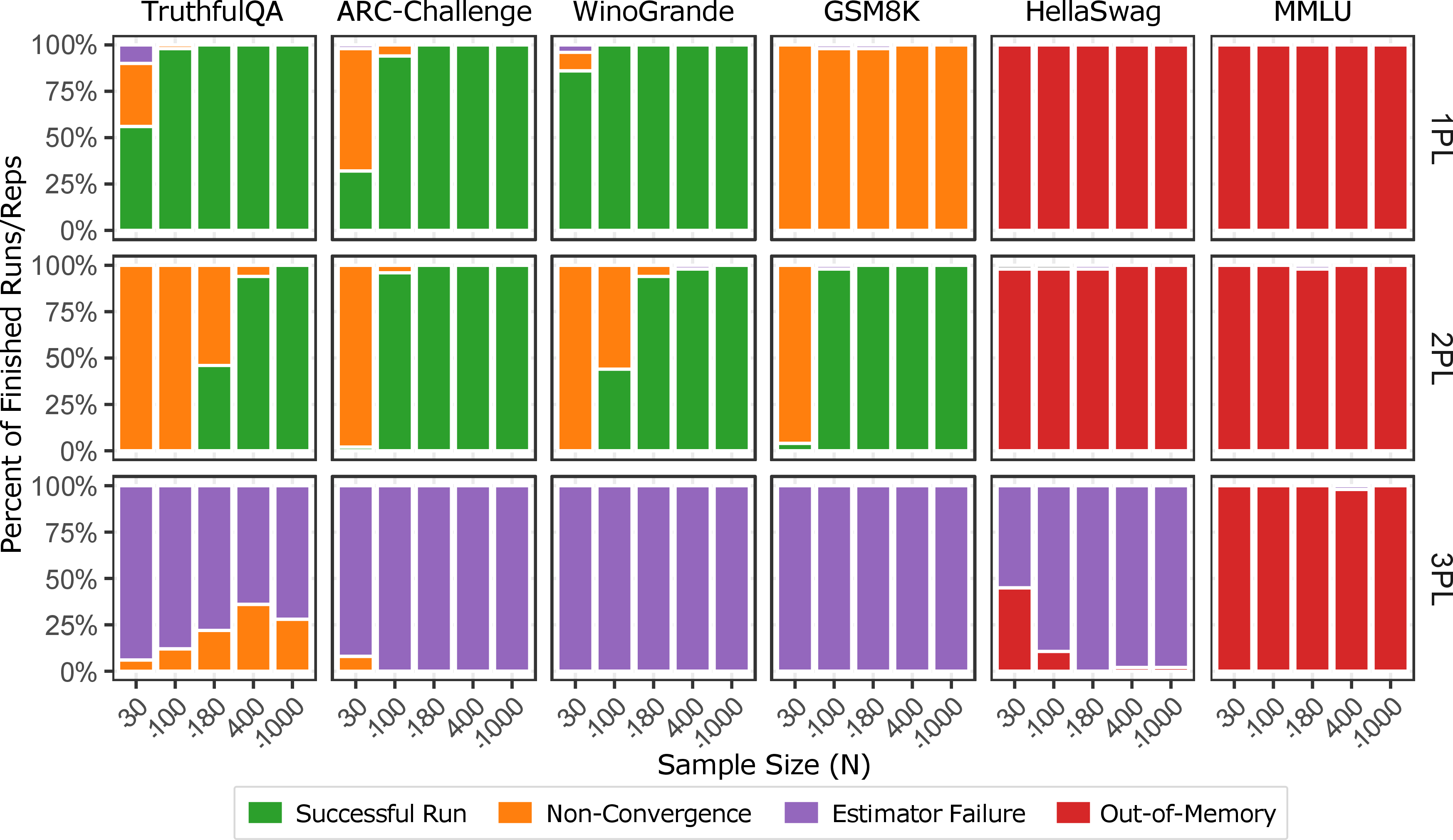
Across all conditions and replications, MML-EM exhibited the highest failure rate (69.45%). Specifically, for HellaSwag and MMLU with \(J>\) 5,000, MML-EM consistently ran out of memory on 32GB CPU RAM. The out-of-memory error persisted on one tested replication with 128GB CPU RAM with HellaSwag, 1PL, \(N = 30\) , rendering it infeasible for large-scale benchmarks. 3PL conditions consistently showed estimation or convergence failures. For smaller benchmarks under 1PL and 2PL, MML-EM often ran into convergence failure small sample sizes. Fig. 12 in App. 10 details the distribution of MML-EM exit status.
For MCMC, estimation became computationally prohibitive for the larger sample sizes and benchmarks: With a 72-hour limit, no replications finished for MMLU when \(N = 1000\) (under any IRT model) and \(N = 400\) (3PL), and for Hellaswag when \(N=1000\) (3PL). \(5.8\%\) of replications under other MMLU and HellaSwag conditions also hit the 72-hour limit. Less than \(0.1\%\) of the finished replications within 72 hours failed due to algorithm divergence.
VI had an overall failure rate of 10.71%. All failures were estimation algorithm failures, primarily in the 3PL conditions (27.56% of replications), with slightly higher rates for larger benchmarks. PSN achieved 0% failure across all conditions.
Runtime differed substantially across estimators (Fig. 2). As 1PL, 2PL, and 3PL did not differ meaningfully in runtime within each estimator, we report averages across IRT models and replications. Note that the reported averages are rough summaries, as wall-clock time depends on hardware configuration: MML-EM, MCMC, and VI were run on CPU, while PSN was run primarily on a single A100 GPU, with a small number of replications on H100 and V100. VI was the fastest estimator with minimal sensitivity to sample size and benchmark length; MCMC was the slowest, often exceeding 10,000 seconds per replication; and PSN runtime scaled with both benchmark length and sample size, growing steeply for large benchmarks; while manageable in our conditions, its scalability to very large benchmarks and samples warrants caution.
5.2 How do different IRT estimators recover model capabilities and rankings?↩︎
We next examined how well each IRT estimator recovered true model capabilities and rankings.
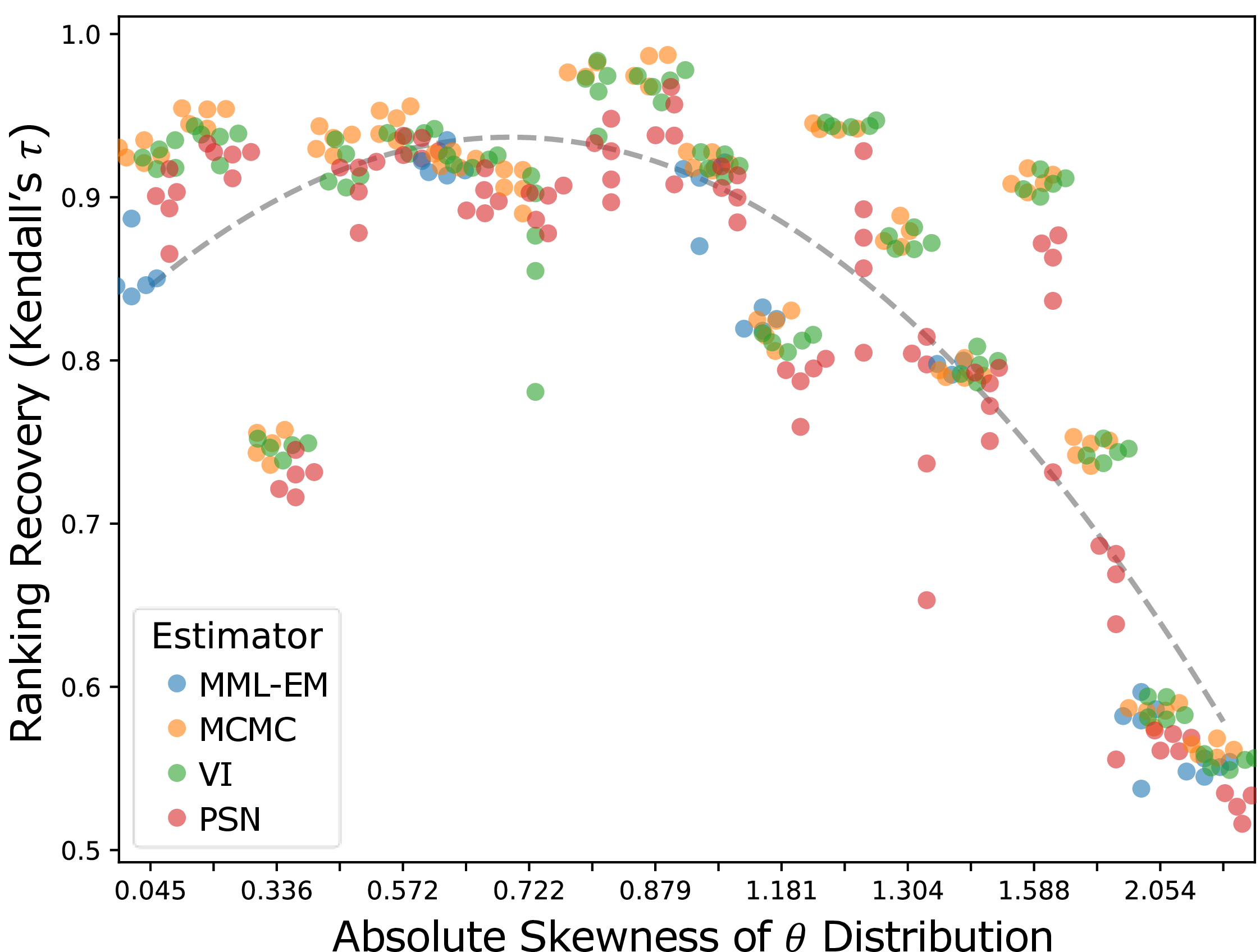
Confirming our concern about the distributional mismatch, the dominant factor affecting ranking recovery was the skewness of the true capability distribution, as revealed in Fig. 3. Conditions (Benchmark \(\times\) IRT model) are sorted from left to right by absolute sample skewness \(\gamma\) [62]. Across all estimators, the ranking recovery exceeded 0.85 for conditions with low skewness (\(|\gamma|\)<0.5), but degraded substantially as skewness increased, falling below 0.60 for the most skewed conditions (\(|\gamma|\)>2.0).
Differences between estimators were comparatively minor. VI (green) achieved slightly higher ranking recovery in most conditions, while PSN (red) tended to underperform relative to the other estimators; However, these differences were small compared to the effect of distributional skewness: even the best-performing estimator produced poor rankings when the underlying ability distribution was highly skewed.
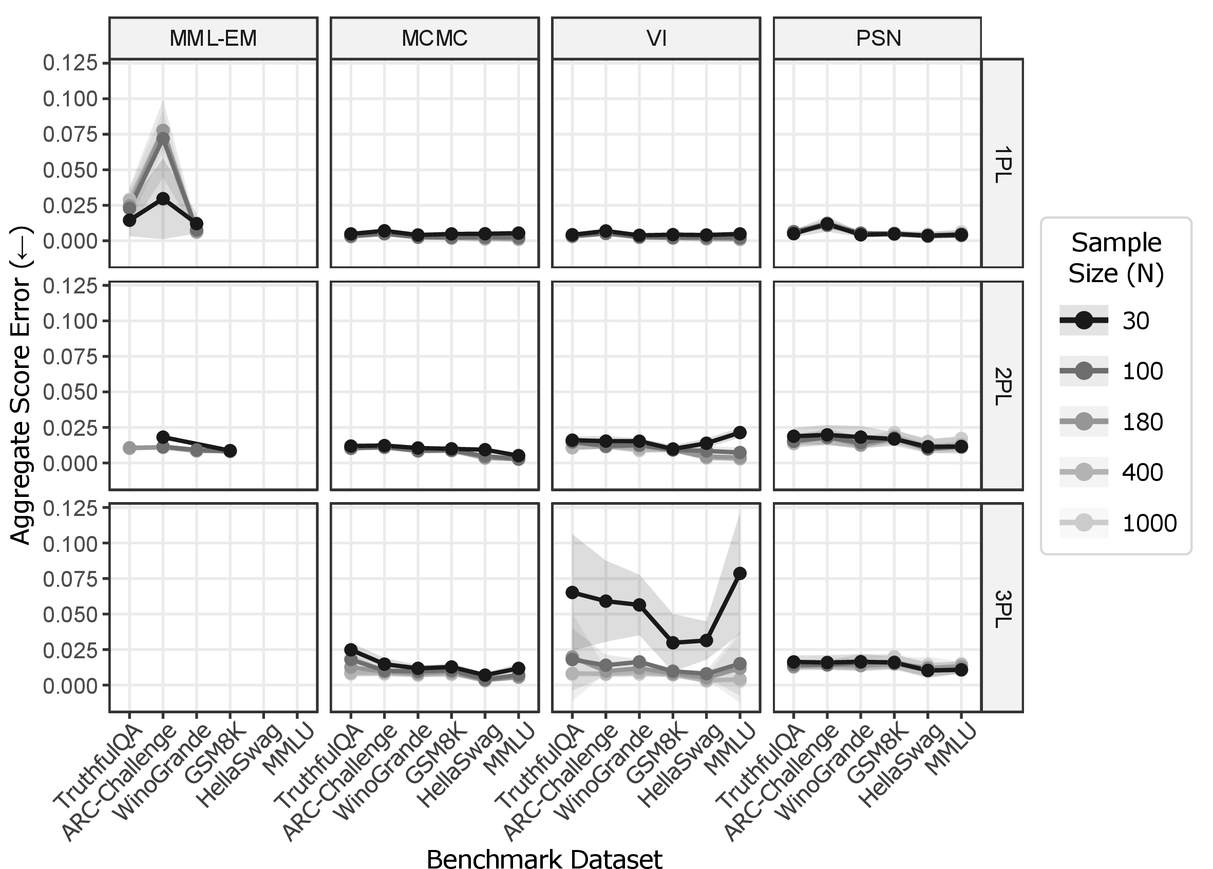
Aggregate score error (Fig. 13 in App. 11.1) was generally low across estimators, with an average deviation of less than .025 from ground truth-implied aggregate score for most conditions under 2PL; However, EM under 1PL and VI under 3PL showed notably elevated errors and high variance, particularly at small sample sizes.
5.3 How do different IRT estimators recover item and benchmark characteristics?↩︎
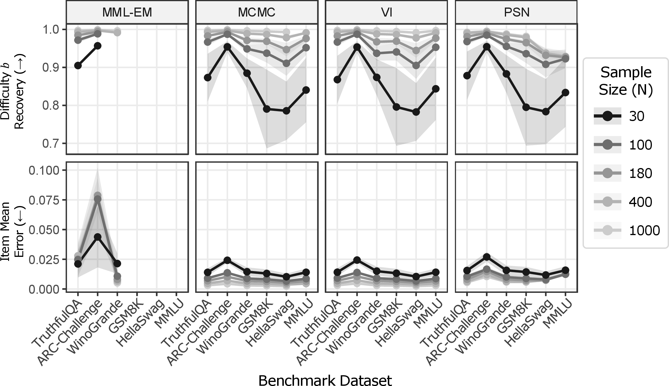
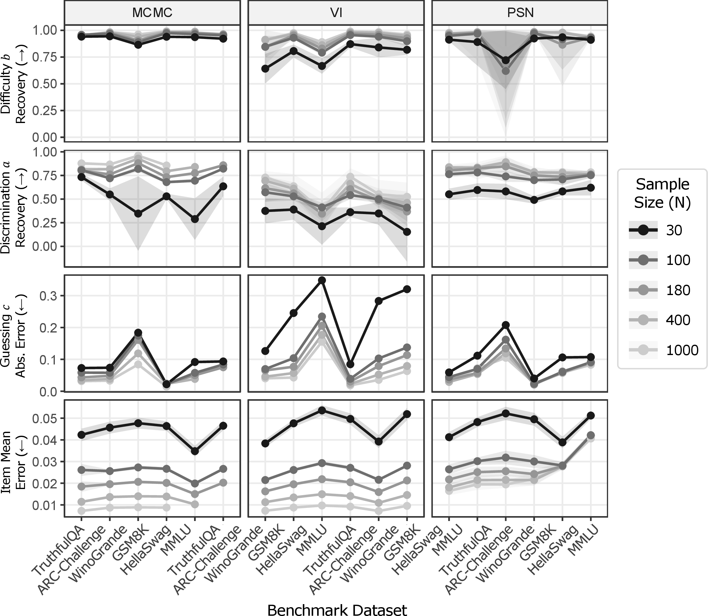
Here, we focus on results under 2PL as the commonly adopted IRT specification in AI benchmarking literature. Fig. 5 presents the difficulty recovery, discrimination recovery, and item mean error across estimators, benchmarks, and sample sizes. Full results for 1/3PL are reported in App. 11.2.
Reliable estimation of item parameters depended heavily on sample size, i.e., the number of evaluated models: \(N\) = 30 (the darkest lines) was insufficient for reliable item parameter recovery under any estimator. At this sample size, difficulty recovery dropped below 0.50 (e.g., MML-EM on ARC-Challenge and PSN on WinoGrande) and discrimination recovery below 0.60 (e.g., MML-EM and PSN on GSM8K), with substantially higher item mean error compared to all larger sample sizes. A marked improvement occurred at \(N\) = 100, though further increasing sample size led to small incremental gains. This suggests that the small model counts (\(N<100\)) typical of AI benchmarking observed in Sec. 3 could risk item-level inference quality, but that even modest increases in sample size can yield substantial improvements.

Among the IRT estimators, MCMC generally achieved the most reliable item parameter recovery when computationally feasible. VI, despite being one of the most widely used estimators in recent IRT-based AI evaluation studies, showed notably unreliable difficulty recovery in several conditions: For 2PL, its difficulty recovery was below \(.5\) for \(N\leq 180\) on TruthfulQA and GSM8K, indicating that VI-estimated item difficulties may diverge substantially from true item difficulty. Simialrly, for MML-EM, the conventional approach to IRT estimation in human testing (small \(J\), large \(N\) regimes), even when it converged, produced unreliable estimates for smaller samples and select benchmarks. PSN, in general, showed more reliable parameter recovery than MML-EM and PSN, with slightly lower accuracy and higher variability across replications than MCMC in some conditions.

5.4 Can estimated IRT parameters support efficient benchmarking?↩︎
Finally, we examined whether short benchmarks, constructed based on expected Fisher information using estimated item parameters, could accurately predict aggregate score on the full test for held-out samples. A random baseline (purple, averaged over 30 random subsets of 10% of the full benchmark per replication) was included for comparison.
As shown in Fig. 4, IRT-based benchmark compression consistently outperformed the random baseline across benchmarks and estimators, though the margin was modest. Neither sample size nor the choice of estimator had a strong effect on short-form ranking recovery, supposing that coarse discrimination estimates might be sufficient to identify relatively informative items. Unlike full-benchmark ranking recovery (Fig. 3), short-form ranking recovery showed no monotonic relationship with the skewness of capability distribution. The factors driving short-form ranking quality thus remain unclear and are left for future investigation.
6 Practical recommendations and implications↩︎
Our results suggest that IRT-based AI benchmark analysis requires different safeguards depending on the intended use of the fitted model. For estimator choice, MML is the conventional approach in human testing, but in our simulations it became computationally burdensome for large-item benchmarks and did not always yield reliable estimates even when runs converged. MCMC provided the most consistent parameter recovery, but its computational cost limited its feasibility for combinations of large benchmarks, large sample sizes, and more complex IRT models. VI was fast and recovered model rankings slightly better, but was found unreliable sometimes for aggregate score recovery and item-parameter recovery. PSN-IRT remained computationally manageable and showed competitive performance in some settings, suggesting that neural estimators may be useful for very large benchmarks, provided their parameter estimates are empirically validated.
Sample size requirements depends on the inference target. Item analysis claims are less reliable for small model pools. In particular, \(N=30\) was insufficient for recovering item difficulty and discrimination across methods, whereas recovery improved clearly at \(N\geq100\). This finding cautions against use of item parameters to characterize item difficulty, informativeness or benchmark quality when sample size is very small. Model-level aggregate performance was less sensitive to sample size when benchmarks were long, as averaging across many items stabilized expected scores. Thus, small model pools may support rough aggregate performance recovery in some settings but could be insufficient for item-quality analysis or benchmark auditing.
Model ranking depended heavily on the shape of the capability distribution. Highly skewed or clustered model populations produced poor rank recovery, likely because ceiling or floor effects leave too few informative items in regions where many models are concentrated. For ranking claims, researchers may consider running simulation checks using their estimated capability and item parameters as a true data-generating model to assess whether rankings are recoverable under the observed sample size, item pool and capability distribution.
7 Limitations and Conclusion↩︎
This paper investigated the reliability of IRT when applied under the data regimes typical of AI benchmarking. Through a structured review of existing studies, we identified substantial heterogeneity in IRT model choices, estimation methods, and data conditions, with many studies operating in regimes far from those for which IRT was originally validated. Our simulation study, spanning 18,000 conditions across six benchmarks, three IRT models, and four estimators, revealed several findings with practical implications.
Several limitations should be noted. Computational feasibility was not assessed on uniform hardware, preventing precise infeasibility thresholds. The factors driving short-form benchmark quality remain unclear despite IRT-based item selection consistently outperforming random baselines. Further, sample sizes between \(30\) and \(100\) were not examined. Estimation algorithm convergence was only monitored under EM. And simulations were restricted to unidimensional IRT models. Our analysis also did not incorporate benchmark-specific information such as item content or semantic features, which may affect item quality in ways that response matrices alone cannot capture. We leave these open questions for future investigation.
To conclude, our findings validate the concern that data regime mismatches between human testing and AI benchmarking have tangible consequences for IRT-based evaluative inferences, which, prior to this work, remained underexamined. Our work demonstrated that the validation practices based on simulation studies could help provide guidance on best practices, data requirements, and potential pitfalls in the statistical analysis of AI benchmarks. As AI benchmarks increasingly inform high-stakes decisions about model deployment and governance, ensuring the measurement tools themselves are reliable in this context is essential. Although this paper only offers concrete guidance for a limited number of scenarios, we envision the simulation methods adopted here to generalize to many other scenarios.
8 Estimator introduction↩︎
8.0.0.1 MML-EM.
Marginal maximum likelihood (MML) is the conventional approach to IRT parameter estimation for human testing. It treats latent traits as random draws from a population distribution, often standard normal for computational convenience, and estimates item
parameters, (\(\boldsymbol{\zeta}_j, j = 1, \ldots, J\)) by maximizing the marginal likelihood given the response matrix: \[L_{MML}(\boldsymbol{\zeta}) =
\prod_{i=1}^{N} \int \left[
\prod_{j=1}^{J} p(Y_{ij} \mid \theta, \boldsymbol{\zeta}_j)
\right]
f(\theta)\, d\theta .\] Optimization is done with the EM algorithm. We used the mirt package and adopted the stochastic variant, the Metropolis-Hastings Robbins-Monro algorithm, replacing fixed quadrature with Monte Carlo integration
when standard EM is too costly for large item pools. Statistical consistency theory guarantees the MML estimator to recover true item parameters when the number of items (\(J\)) is fixed and sample size (\(N\)) grows to infinity. Although in human testing, often the assumption of trait normality is empirically plausible and \(J<N\), MML’s behavior is less certain in AI benchmark regimes, where
the number of evaluated systems may be small, the number of items large, and the capability distribution nonnormal.
8.0.0.2 MCMC.
Bayesian MCMC specifies prior distributions for item parameters and model capabilities, and then samples from the posterior distribution after observing the response data (\(\mathbf{Y}\)),
\[\label{eq:bayes95post}
p(\boldsymbol{\theta},\boldsymbol{\zeta}\mid Y)
\propto
p(Y\mid \boldsymbol{\theta},\boldsymbol{\zeta})
p(\boldsymbol{\theta},\boldsymbol{\zeta}).\tag{1}\] We implemented Bayesian estimation in brms, which uses Stan’s Hamiltonian Monte Carlo sampler. HMC uses gradient information to reduce random-walk behavior, although sampling
efficiency still depends on posterior geometry and model size. Prior settings and implementation details are reported in Appendix A. Bayesian posterior estimates can be sensitive to prior specification when empirical information is limited, especially when
few evaluated systems are available for estimating many item parameters. Further, runtime grows with both sample size and benchmark length as each MCMC iteration evaluates the full likelihood over all model and item parameters. The prior specifications for
the MCMC algorithm in this study followed [63] and are summarized in Table 1. For each
model, the MCMC algorithm was run using a single chain with 2,000 total iterations, where the first 1,000 iterations were discarded as burn-in.
8.0.0.3 Variational inference.
VI in this study was fitted with py-irt, which approximates the Bayesian posterior in Equation 1 with a tractable variational distribution, e.g., for the 1PL model,
\[\label{eq:vi95dist}
q_{\phi}(\boldsymbol{\theta},\mathbf{b},\mu,\tau)=
q(\mu)q(\tau)\prod_{i=1}^{N}q(\theta_i)\prod_{j=1}^{J}q(b_j),\tag{2}\] where \(\mu\) and \(\tau\) are the location and precision parameters of the normal latent capability. The
variational parameters are estimated by minimizing \(D_{\mathrm{KL}}(q_{\phi}\,\|\,p)\), the KL divergence between 2 and 1 . VI is computationally attractive
for long benchmark matrices as it replaces numerical integration or posterior sampling with gradient-based optimization. However, it inherits the prior assumptions of the Bayesian model and adds approximation error from the chosen variational family, which
can affect inferences in small-sample AI benchmark settings and when capability distributions is nonnormal.
8.0.0.4 PSN-IRT.
PSN [12] is a neural-network representation of an IRT model, which assigns each evaluated model a learned capability embedding (\(\theta_i\)) and each benchmark item item-parameter embeddings \((a_j,b_j,c_j)\). These embeddings are passed through an item response function layer to predict binary response. We adapted the authors’ original 4PL implementation to the 1 - 3PL models used in our simulation. PSN is computationally efficient with gradient-based optimization and does not assuming a normal distribution for latent capability. However, it is trained as a predictive neural model and does not directly provide uncertainty quantification or parameter consistency guarantees for parameter estimates, and its estimates are specific to the trained network and item set.
| IRT Model | Parameter | Prior | Hyperprior |
|---|---|---|---|
| 1PL | Ability (\(\theta\)) | \(\theta_i\!\sim\!\text{Normal}(0, \sigma_\theta)\) | \(\sigma_\theta\!\sim\!\text{Normal}^+(0, 1)\) |
| 2-4 | Difficulty (\(b\)) | \(b_j\!\sim\!\text{Normal}(\mu_b, \sigma_b)\) | \(\sigma_b\!\sim\!\text{Normal}^+(0, 3)\) |
| 2PL & 3PL | Ability (\(\theta\)) | \(\theta_i\!\sim\!\text{Normal}(0, 1)\) | \(\sigma_\theta = 1\) (Fixed scale) |
| 2-4 | Difficulty (\(b\)) | \(b_j\!\sim\!\text{Normal}(\mu_b, \sigma_b)\) | \(\mu_b\!\sim\!\text{Normal}(0, 5)\) \(\sigma_b\!\sim\!\text{Normal}^+(0, 3)\) |
| 2-4 | Discrimination (\(a\)) | \(\log a_j\!\sim\!\text{Normal}(\mu_{\log a}, \sigma_{\log a})\) | \(\mu_{\log a}\!\sim\!\text{Normal}(0, 1)\) \(\sigma_{\log a}\!\sim\!\text{Normal}^+(0, 1)\) |
| 3PL | Pseudo-Guessing (\(c\)) | \(\text{logit } c_j\!\sim\!\text{Normal}(\mu_{\text{logit } c}, \sigma_{\text{logit } c})\) | \(\mu_{\text{logit } c}\!\sim\!\text{Logistic}(0, 1)\) \(\sigma_{\text{logit } c}\!\sim\!\text{Normal}^+(0, 1)\) |
9 True capability and difficulty distributions↩︎
In Figs. 6–11, we present distributions of true capability (\(\theta\)) and difficulty (\(b\)) parameters for the six benchmarks under 1PL, 2PL, and 3PL models, estimated from the full OpenLLM response matrices via variational inference. All distributions exhibit non-normality, with capability values showing multimodality across all three IRT models.
10 Exit statuses of MML-EM↩︎
The distribution of the exit statuses is displayed in Fig. 12.
11 Detailed results for parameter recovery↩︎
11.1 Aggregate score error↩︎
Please refer to Fig. 13 for detailed results.
11.2 Item parameter recovery↩︎
Please refer to Figs. 14 & 15 for detailed results.
NeurIPS Paper Checklist↩︎
The checklist is designed to encourage best practices for responsible machine learning research, addressing issues of reproducibility, transparency, research ethics, and societal impact. Do not remove the checklist: The papers not including the checklist will be desk rejected. The checklist should follow the references and follow the (optional) supplemental material. The checklist does NOT count towards the page limit.
Please read the checklist guidelines carefully for information on how to answer these questions. For each question in the checklist:
You should answer , , or .
means either that the question is Not Applicable for that particular paper or the relevant information is Not Available.
Please provide a short (1–2 sentence) justification right after your answer (even for ).
The checklist answers are an integral part of your paper submission. They are visible to the reviewers, area chairs, senior area chairs, and ethics reviewers. You will also be asked to include it (after eventual revisions) with the final version of your paper, and its final version will be published with the paper.
The reviewers of your paper will be asked to use the checklist as one of the factors in their evaluation. While is generally preferable to , it is perfectly acceptable to answer provided a proper justification is given (e.g., error bars are not reported because it would be too computationally expensive” or “we were unable to find the license for the dataset we used”). In general, answering or is not grounds for rejection. While the questions are phrased in a binary way, we acknowledge that the true answer is often more nuanced, so please just use your best judgment and write a justification to elaborate. All supporting evidence can appear either in the main paper or the supplemental material, provided in appendix. If you answer to a question, in the justification please point to the section(s) where related material for the question can be found.
IMPORTANT, please:
Delete this instruction block, but keep the section heading “NeurIPS Paper Checklist",
Keep the checklist subsection headings, questions/answers and guidelines below.
Do not modify the questions and only use the provided macros for your answers.
Claims
Question: Do the main claims made in the abstract and introduction accurately reflect the paper’s contributions and scope?
Answer:
Justification: The abstract and introduction state three contributions: (1) a literature review of IRT adoption in AI evaluation, (2) a simulation study calibrated to AI evaluation conditions, and (3) practical guidance for IRT-based AI evaluation. These are delivered in Secs. 3, 4–5, and 6, respectively.
Guidelines:
The answer means that the abstract and introduction do not include the claims made in the paper.
The abstract and/or introduction should clearly state the claims made, including the contributions made in the paper and important assumptions and limitations. A or answer to this question will not be perceived well by the reviewers.
The claims made should match theoretical and experimental results, and reflect how much the results can be expected to generalize to other settings.
It is fine to include aspirational goals as motivation as long as it is clear that these goals are not attained by the paper.
Limitations
Question: Does the paper discuss the limitations of the work performed by the authors?
Answer:
Justification: Limitations are discussed in Sec. 7.
Guidelines:
The answer means that the paper has no limitation while the answer means that the paper has limitations, but those are not discussed in the paper.
The authors are encouraged to create a separate “Limitations” section in their paper.
The paper should point out any strong assumptions and how robust the results are to violations of these assumptions (e.g., independence assumptions, noiseless settings, model well-specification, asymptotic approximations only holding locally). The authors should reflect on how these assumptions might be violated in practice and what the implications would be.
The authors should reflect on the scope of the claims made, e.g., if the approach was only tested on a few datasets or with a few runs. In general, empirical results often depend on implicit assumptions, which should be articulated.
The authors should reflect on the factors that influence the performance of the approach. For example, a facial recognition algorithm may perform poorly when image resolution is low or images are taken in low lighting. Or a speech-to-text system might not be used reliably to provide closed captions for online lectures because it fails to handle technical jargon.
The authors should discuss the computational efficiency of the proposed algorithms and how they scale with dataset size.
If applicable, the authors should discuss possible limitations of their approach to address problems of privacy and fairness.
While the authors might fear that complete honesty about limitations might be used by reviewers as grounds for rejection, a worse outcome might be that reviewers discover limitations that aren’t acknowledged in the paper. The authors should use their best judgment and recognize that individual actions in favor of transparency play an important role in developing norms that preserve the integrity of the community. Reviewers will be specifically instructed to not penalize honesty concerning limitations.
Theory assumptions and proofs
Question: For each theoretical result, does the paper provide the full set of assumptions and a complete (and correct) proof?
Answer:
Justification: Assumptions and empirical evidence are discussed and provided in Sec. 5.
Guidelines:
The answer means that the paper does not include theoretical results.
All the theorems, formulas, and proofs in the paper should be numbered and cross-referenced.
All assumptions should be clearly stated or referenced in the statement of any theorems.
The proofs can either appear in the main paper or the supplemental material, but if they appear in the supplemental material, the authors are encouraged to provide a short proof sketch to provide intuition.
Inversely, any informal proof provided in the core of the paper should be complemented by formal proofs provided in appendix or supplemental material.
Theorems and Lemmas that the proof relies upon should be properly referenced.
Experimental result reproducibility
Question: Does the paper fully disclose all the information needed to reproduce the main experimental results of the paper to the extent that it affects the main claims and/or conclusions of the paper (regardless of whether the code and data are provided or not)?
Answer:
Justification: Implementation details are comprehensively discussed in both Sec. 3 and App. 8.
Guidelines:
The answer means that the paper does not include experiments.
If the paper includes experiments, a answer to this question will not be perceived well by the reviewers: Making the paper reproducible is important, regardless of whether the code and data are provided or not.
If the contribution is a dataset and/or model, the authors should describe the steps taken to make their results reproducible or verifiable.
Depending on the contribution, reproducibility can be accomplished in various ways. For example, if the contribution is a novel architecture, describing the architecture fully might suffice, or if the contribution is a specific model and empirical evaluation, it may be necessary to either make it possible for others to replicate the model with the same dataset, or provide access to the model. In general. releasing code and data is often one good way to accomplish this, but reproducibility can also be provided via detailed instructions for how to replicate the results, access to a hosted model (e.g., in the case of a large language model), releasing of a model checkpoint, or other means that are appropriate to the research performed.
While NeurIPS does not require releasing code, the conference does require all submissions to provide some reasonable avenue for reproducibility, which may depend on the nature of the contribution. For example
If the contribution is primarily a new algorithm, the paper should make it clear how to reproduce that algorithm.
If the contribution is primarily a new model architecture, the paper should describe the architecture clearly and fully.
If the contribution is a new model (e.g., a large language model), then there should either be a way to access this model for reproducing the results or a way to reproduce the model (e.g., with an open-source dataset or instructions for how to construct the dataset).
We recognize that reproducibility may be tricky in some cases, in which case authors are welcome to describe the particular way they provide for reproducibility. In the case of closed-source models, it may be that access to the model is limited in some way (e.g., to registered users), but it should be possible for other researchers to have some path to reproducing or verifying the results.
Open access to data and code
Question: Does the paper provide open access to the data and code, with sufficient instructions to faithfully reproduce the main experimental results, as described in supplemental material?
Answer:
Justification: The study is primarily build on existing IRT-based evaluation practices and does not release new data or code.
Guidelines:
The answer means that paper does not include experiments requiring code.
Please see the NeurIPS code and data submission guidelines (https://neurips.cc/public/guides/CodeSubmissionPolicy) for more details.
While we encourage the release of code and data, we understand that this might not be possible, so is an acceptable answer. Papers cannot be rejected simply for not including code, unless this is central to the contribution (e.g., for a new open-source benchmark).
The instructions should contain the exact command and environment needed to run to reproduce the results. See the NeurIPS code and data submission guidelines (https://neurips.cc/public/guides/CodeSubmissionPolicy) for more details.
The authors should provide instructions on data access and preparation, including how to access the raw data, preprocessed data, intermediate data, and generated data, etc.
The authors should provide scripts to reproduce all experimental results for the new proposed method and baselines. If only a subset of experiments are reproducible, they should state which ones are omitted from the script and why.
At submission time, to preserve anonymity, the authors should release anonymized versions (if applicable).
Providing as much information as possible in supplemental material (appended to the paper) is recommended, but including URLs to data and code is permitted.
Experimental setting/details
Question: Does the paper specify all the training and test details (e.g., data splits, hyperparameters, how they were chosen, type of optimizer) necessary to understand the results?
Answer:
Justification: Implementation details are comprehensively discussed in both Sec. 3 and App. 8.
Guidelines:
The answer means that the paper does not include experiments.
The experimental setting should be presented in the core of the paper to a level of detail that is necessary to appreciate the results and make sense of them.
The full details can be provided either with the code, in appendix, or as supplemental material.
Experiment statistical significance
Question: Does the paper report error bars suitably and correctly defined or other appropriate information about the statistical significance of the experiments?
Answer:
Justification: All results are aggregated over 50 replications per condition. Figures report means with \(\pm\)1 standard deviation as shaded regions or error bars.
Guidelines:
The answer means that the paper does not include experiments.
The authors should answer if the results are accompanied by error bars, confidence intervals, or statistical significance tests, at least for the experiments that support the main claims of the paper.
The factors of variability that the error bars are capturing should be clearly stated (for example, train/test split, initialization, random drawing of some parameter, or overall run with given experimental conditions).
The method for calculating the error bars should be explained (closed form formula, call to a library function, bootstrap, etc.)
The assumptions made should be given (e.g., Normally distributed errors).
It should be clear whether the error bar is the standard deviation or the standard error of the mean.
It is OK to report 1-sigma error bars, but one should state it. The authors should preferably report a 2-sigma error bar than state that they have a 96% CI, if the hypothesis of Normality of errors is not verified.
For asymmetric distributions, the authors should be careful not to show in tables or figures symmetric error bars that would yield results that are out of range (e.g., negative error rates).
If error bars are reported in tables or plots, the authors should explain in the text how they were calculated and reference the corresponding figures or tables in the text.
Experiments compute resources
Question: For each experiment, does the paper provide sufficient information on the computer resources (type of compute workers, memory, time of execution) needed to reproduce the experiments?
Answer:
Justification: It is discussed in Sec. 5.1 on computational feasibility.
Guidelines:
The answer means that the paper does not include experiments.
The paper should indicate the type of compute workers CPU or GPU, internal cluster, or cloud provider, including relevant memory and storage.
The paper should provide the amount of compute required for each of the individual experimental runs as well as estimate the total compute.
The paper should disclose whether the full research project required more compute than the experiments reported in the paper (e.g., preliminary or failed experiments that didn’t make it into the paper).
Code of ethics
Question: Does the research conducted in the paper conform, in every respect, with the NeurIPS Code of Ethics https://neurips.cc/public/EthicsGuidelines?
Answer:
Justification: Yes, this study was conducted in accordance with the code of ethics.
Guidelines:
The answer means that the authors have not reviewed the NeurIPS Code of Ethics.
If the authors answer , they should explain the special circumstances that require a deviation from the Code of Ethics.
The authors should make sure to preserve anonymity (e.g., if there is a special consideration due to laws or regulations in their jurisdiction).
Broader impacts
Question: Does the paper discuss both potential positive societal impacts and negative societal impacts of the work performed?
Answer:
Guidelines:
The answer means that there is no societal impact of the work performed.
If the authors answer or , they should explain why their work has no societal impact or why the paper does not address societal impact.
Examples of negative societal impacts include potential malicious or unintended uses (e.g., disinformation, generating fake profiles, surveillance), fairness considerations (e.g., deployment of technologies that could make decisions that unfairly impact specific groups), privacy considerations, and security considerations.
The conference expects that many papers will be foundational research and not tied to particular applications, let alone deployments. However, if there is a direct path to any negative applications, the authors should point it out. For example, it is legitimate to point out that an improvement in the quality of generative models could be used to generate Deepfakes for disinformation. On the other hand, it is not needed to point out that a generic algorithm for optimizing neural networks could enable people to train models that generate Deepfakes faster.
The authors should consider possible harms that could arise when the technology is being used as intended and functioning correctly, harms that could arise when the technology is being used as intended but gives incorrect results, and harms following from (intentional or unintentional) misuse of the technology.
If there are negative societal impacts, the authors could also discuss possible mitigation strategies (e.g., gated release of models, providing defenses in addition to attacks, mechanisms for monitoring misuse, mechanisms to monitor how a system learns from feedback over time, improving the efficiency and accessibility of ML).
Safeguards
Question: Does the paper describe safeguards that have been put in place for responsible release of data or models that have a high risk for misuse (e.g., pre-trained language models, image generators, or scraped datasets)?
Answer:
Justification: The study is primarily build on existing IRT-based evaluation practices and does not release new data or code.
Guidelines:
The answer means that the paper poses no such risks.
Released models that have a high risk for misuse or dual-use should be released with necessary safeguards to allow for controlled use of the model, for example by requiring that users adhere to usage guidelines or restrictions to access the model or implementing safety filters.
Datasets that have been scraped from the Internet could pose safety risks. The authors should describe how they avoided releasing unsafe images.
We recognize that providing effective safeguards is challenging, and many papers do not require this, but we encourage authors to take this into account and make a best faith effort.
Licenses for existing assets
Question: Are the creators or original owners of assets (e.g., code, data, models), used in the paper, properly credited and are the license and terms of use explicitly mentioned and properly respected?
Answer:
Justification: All used artifacts are open-sourced, explicitly mentioned, and correctly cited.
Guidelines:
The answer means that the paper does not use existing assets.
The authors should cite the original paper that produced the code package or dataset.
The authors should state which version of the asset is used and, if possible, include a URL.
The name of the license (e.g., CC-BY 4.0) should be included for each asset.
For scraped data from a particular source (e.g., website), the copyright and terms of service of that source should be provided.
If assets are released, the license, copyright information, and terms of use in the package should be provided. For popular datasets, paperswithcode.com/datasets has curated licenses for some datasets. Their licensing guide can help determine the license of a dataset.
For existing datasets that are re-packaged, both the original license and the license of the derived asset (if it has changed) should be provided.
If this information is not available online, the authors are encouraged to reach out to the asset’s creators.
New assets
Question: Are new assets introduced in the paper well documented and is the documentation provided alongside the assets?
Answer:
Justification: The study is primarily build on existing IRT-based evaluation practices and does not release new assets.
Guidelines:
The answer means that the paper does not release new assets.
Researchers should communicate the details of the dataset/code/model as part of their submissions via structured templates. This includes details about training, license, limitations, etc.
The paper should discuss whether and how consent was obtained from people whose asset is used.
At submission time, remember to anonymize your assets (if applicable). You can either create an anonymized URL or include an anonymized zip file.
Crowdsourcing and research with human subjects
Question: For crowdsourcing experiments and research with human subjects, does the paper include the full text of instructions given to participants and screenshots, if applicable, as well as details about compensation (if any)?
Answer:
Justification: The paper does not involve crowdsourcing nor research with human subjects.
Guidelines:
The answer means that the paper does not involve crowdsourcing nor research with human subjects.
Including this information in the supplemental material is fine, but if the main contribution of the paper involves human subjects, then as much detail as possible should be included in the main paper.
According to the NeurIPS Code of Ethics, workers involved in data collection, curation, or other labor should be paid at least the minimum wage in the country of the data collector.
Institutional review board (IRB) approvals or equivalent for research with human subjects
Question: Does the paper describe potential risks incurred by study participants, whether such risks were disclosed to the subjects, and whether Institutional Review Board (IRB) approvals (or an equivalent approval/review based on the requirements of your country or institution) were obtained?
Answer:
Justification: The paper does not involve crowdsourcing nor research with human subjects.
Guidelines:
The answer means that the paper does not involve crowdsourcing nor research with human subjects.
Depending on the country in which research is conducted, IRB approval (or equivalent) may be required for any human subjects research. If you obtained IRB approval, you should clearly state this in the paper.
We recognize that the procedures for this may vary significantly between institutions and locations, and we expect authors to adhere to the NeurIPS Code of Ethics and the guidelines for their institution.
For initial submissions, do not include any information that would break anonymity (if applicable), such as the institution conducting the review.
Declaration of LLM usage
Question: Does the paper describe the usage of LLMs if it is an important, original, or non-standard component of the core methods in this research? Note that if the LLM is used only for writing, editing, or formatting purposes and does not impact the core methodology, scientific rigor, or originality of the research, declaration is not required.
Answer:
Justification: The core method development (simulation study) in this research does not involve LLMs as any important, original, or non-standard components.
Guidelines:
The answer means that the core method development in this research does not involve LLMs as any important, original, or non-standard components.
Please refer to our LLM policy in the NeurIPS handbook for what should or should not be described.