Evaluating covariate balance for long time horizon Markov decision processes
July 16, 2026
Abstract
This article explores the application of covariate balance diagnostics for detecting the presence of hidden confounding/model miss-specification in studies applying offline reinforcement learning (RL) to deriving optimal treatment recommendations. The
results demonstrate that, either there is a high risk of bias within existing offline RL studies for treatment recommendations or, existing covariate balance metrics are not sufficient to assess such studies. Regardless, existing offline RL studies cannot
be concluded as being statistically robust. The conclusions propose future research directions for obtaining more methodologically robust applications of offline RL to treatment recommendation problems.
Keywords: Off-policy evaluation, offline reinforcement learning, observational healthcare data, sepsis management
1 Introduction↩︎
Offline reinforcement learning (RL) has become increasingly popular within the artificial intelligence (AI) community for various domains, including robotics, healthcare and power plant control. Some of these domains, a notable example being healthcare,
assume the analysis is performed entirely offline i.e., there is no ability to obtain on-policy trajectories (outside of behaviour cloning). These domains rely on off-policy evaluation (OPE) to obtain quantitative measures of performance.
OPE is a causal inference problem in the sense that the assumptions are equivalent ([@Chakraborty2013]). Under OPE (or offline RL), a Markov decision process (MPD), or variant thereof, is assumed
whilst, for causal inference analyses, the assumptions of consistency and exchangeability are required. Asserting the correctness of an MDP, or of consistency and exchangeability, is equally unverifiable. Within the context of causal inference, to account
for this lack of verifiability, various diagnostic checks of robustness of causal inferences have been proposed ([@Rubin2001], [@austin_balance_2009]). However, such checks are seldom seen in applications of OPE and offline RL in the AI community.
The primary aim of this analysis was to understand the extent to which existing applications of offline RL within healthcare satisfy the diagnostic checks of assumptions that are common place within the causal inference community. Of particular focus is in
applying the covariate balance diagnostic to applications of offline RL to learning treatment regimens for sepsis.
1.1 Contributions↩︎
The contributions of this analysis are two-fold:
Section 3 consolidates and formalises the definitions of covariate balance and extends the "weighted" version to the time-dependent setting;
Section 4 demonstrates that existing studies applying offline RL to treatment recommendations in healthcare fail to satisfy covariate balance tests. It cannot be determined whether this is a result of confounding/model miss-specification being present or the inappropriateness of the tests for long time horizons. Regardless, the conclusions motivate new research directions within the field.
2 Background↩︎
Research has already been conducted into the application of offline RL to a wide array of domains. In a survey, [@Yu2019] highlighted the following areas of physical health where research has been
conducted: cancer treatment, anemia management of patients requiring dialysis, insulin dosing for diabetic patients, management of HIV, and more recently ICU applications including the treatment of sepsis (via vasosuppressor and IV dosage), optimal
ventilation and optimal glycemic control (again for sepsis management).
Applications of offline RL to sepsis management have, almost exclusively, used the same MDP definition and preprocessing pipeline. Beginning with the seminal paper from [@Komorowski2018], subsequent
papers shared the established preprocessing pipelines developed by Komorowski et al ([@Prasad2017], [@Raghu2018]). The causal question analysed has
been, the causal effect of different dosages of intravenous (IV) fluids and vasopressors on 90 day mortality of adult sepsis patients, with exclusions being applied to palliative patients. Patient trajectories have been defined by 24 hours of observations
prior to sepsis onset and 48 hours proceeding. These trajectories have been discretised into 4 hour buckets, resulting in a maximum 18 step algorithmic horizon. The action space has been defined by discretising IV fluid and vasopressor dosages into 5
buckets each, resulting in a discrete action space of dimension 25. For a more detailed breakdown of the cohort, refer to [@Komorowski2018].
Within causal inference diagnostic checks for confounding/model miss-specification have predominantly revolved around covariate balance assessments using propensity scores ([@Rubin2001], [@austin_balance_2009]). [@Rubin2001] in particular advocated for the use of propensity based methods since there do not require exposure to
outcome data, emulating to some extent the process of a clinical trial. The use of propensity based methods within causal inference is in stark contrast to the offline RL community where, potentially due to recommendations from large simulation studies
([@Fu2021], [@Voloshin2019]), there has been a general focus on outcome based methods. Whilst there is a wider acceptance for the necessity of
covariate balance checks within the causal inference community, definitions of estimators and extensions to the time-dependent setting are not obvious from the literature.
3 Covariate balance↩︎
It will be demonstrated that there exists two distinct notions of covariate balance and these will be referred to as conditional covariate balance and weighted covariate balance. Before proceeding to these definitions however, it is instructive to consider the different types of propensity score based estimators used for performing causal inferences. For the first part of this section, a contextual bandit density (equation 1 ) will be used where \(A\) defines the treatment, \(S\) defines the confounding variables and \(R\) defines the outcome of interest. \[\label{equ:cb95density} p_{\pi}(\tau) = p_{S}(s)p_{\pi}(a|s)p_{R}(r|a,s)\tag{1}\]
3.1 Propensity score estimators for causal inference↩︎
Within causal inference, there exist a number of different types of estimators which utilise the propensity score, and these can be grouped as either conditional or weighting based estimators. This is in contrast to off-policy evaluation in the offline
reinforcement learning literature, where importance sampling (weighting) based estimators are solely used.
Conditioning estimators (i.e., propensity score matching and stratification) utilise theorem 3 of [@rosenbaum_central_1983], reproduced in Theorem 1.
Theorem 1 (Theorem 3 of [@rosenbaum_central_1983]). If treatment assignment is strongly ignorable, then it is strongly ignorable given any balancing score \(b(x)\); that is \(\forall x\), \[\begin{align} (R_{1},R_{0}) \perp \!\!\! \perp A|S \textrm{ and } 0<P(A=1|S)<1 \end{align}\] implies, \(\forall b(x)\): \[\begin{align} (R_{1},R_{0}) \perp \!\!\! \perp A|b(S) \textrm{ and } 0<P(A=1|b(S))<1 \end{align}\]
In short, the theorem states that if positivity and exchangeability (and consistency) hold1 given the covariates, then the potential outcomes and treatments are
exchangeable given any balancing score, where a balancing score is defined as inducing conditional independence between the treatment and covariates (a balancing score is any \(b(s)\) such that: \(A \perp \!\!\! \perp S | b(S)\)).
From theorem 1, and as an example of a conditioning estimator, the propensity score matching estimator can be derived, with \(e(S) = P(A=1|S)\), as: \[\begin{align} \mathbb{E}\big[\mathbb{E}[R^{\mathrm{do}{}(A=1)}-&R^{\mathrm{do}{}(A=0)}|S]\big]
=\mathbb{E}\big[\mathbb{E}[R^{\mathrm{do}{}(A=1)}|S]\big]-\mathbb{E}\big[\mathbb{E}[R^{\mathrm{do}{}(A=0)}|S]\big] \\ = & \mathbb{E}\big[\mathbb{E}[R^{\mathrm{do}{}(A=1)}|S,e(S)]\big]-\mathbb{E}\big[\mathbb{E}[R^{\mathrm{do}{}(A=0)}|S,e(S)]\big]
\tag{2} \\ = & \mathbb{E}\big[\mathbb{E}[R^{\mathrm{do}{}(A=1)}|e(S)]\big]-\mathbb{E}\big[\mathbb{E}[R^{\mathrm{do}{}(A=0)}|e(S)]\big] \tag{3} \\ = &
\mathbb{E}\big[\mathbb{E}[R^{\mathrm{do}{}(A=1)}|A=1,e(S)]\big]-\mathbb{E}\big[\mathbb{E}[R^{\mathrm{do}{}(A=0)}|A=0,e(S)]\big] \tag{4} \\ = & \mathbb{E}\big[\mathbb{E}[R|A=1,e(S)]\big]-\mathbb{E}\big[\mathbb{E}[R|A=0,e(S)]\big] \tag{5}\\ = &
\mathbb{E}\big[\mathbb{E}[R|A=1,e(S)]-\mathbb{E}[R|A=0,e(S)]\big] \tag{6}
\end{align}\]
Where: equation 2 follows as \(e(S)\) is courser than \(S\) ([@rosenbaum_central_1983]); equation 3 follows from theorem 1
and; equations 4 and 5 follow from the assumptions of exchangability and consistency, respectively.
Assuming a dataset \(d=\{(s_{i},a_{i},r_{i})\}_{i=1}^{n}\), generated according to equation 1 . Furthermore, let \(d_{1} = \{(s_{i},a_{i},r_{i}):a_{i}=1,
(s_{i},a_{i},r_{i}) \in d\}\) and \(d_{0} = \{(s_{i},a_{i},r_{i}):a_{i}=0, (s_{i},a_{i},r_{i}) \in d\}\). (One-to-one) matching requires pairing each observation in \(d_{1}\) with an
observation in \(d_{0}\) under the condition that \(e(s_{i}) \approx e(s_{j})\) for the \(i\)th observation in \(d_{1}\) and
the \(j\)th observation in \(d_{0}\). Let \(m=\{(\tau_{i,1},\tau_{i,0}):\tau_{i,1} \in d_{1},\tau_{i,0} \in d_{0},e(s_{i,1})=e(s_{i,0}),s_{i,1}\in \tau_{i,1},
s_{i,0} \in \tau_{i,0}\}\), then, beginning with equation 6 : \[\begin{align} \mathbb{E}\big[\mathbb{E}[R|A=1,e(S)]-\mathbb{E}[R|A=0,e(S)]\big] \approx
\frac{1}{|\mathcal{E}|}\sum_{\mathcal{E}}\Bigg(\frac{1}{|\mathcal{E}_{i}|}\sum_{\mathcal{E}_{i}}r_{i,1}-\frac{1}{|\mathcal{E}_{i}|}\sum_{\mathcal{E}_{i}}r_{i,0}\Bigg)
\end{align}\] where \(\mathcal{E}\) is the unique values of \(e(S)\) in \(d\), such that \(\mathcal{E} = \bigcap
\mathcal{E}_{i}\). Where, for every \(\mathcal{E}_{i}\) there is only one pair of matches, the estimator is equivalent to: \[\begin{align} \frac{1}{|m|}\sum_{i=1}^{|m|}r_{i,1}-r_{i,0}
\end{align}\]
In contrast to conditioning estimators, weighting estimators do not explicitely use the conditional independence statement of theorem 1 and
critically, the derivation does not hold for any balancing score, \(b(s)\): \[\begin{align} \mathbb{E}[R^{\mathrm{do}{}(A=a)}|S] &= \mathbb{E}[R^{\mathrm{do}{}(A=a)}|A=a,S]
\\ &= \mathbb{E}[R|A=a,S] \tag{7}\\ &= \int_{\mathcal{R}} R P(R|A=a,S)\\ &= \int_{\mathcal{R}} R \frac{P(R,A=a,S)}{P(A=a,S)} \\ &= \int_{\mathcal{R}} \frac{R}{P(A=a|S)}\frac{P(R,A=a,S)}{P(S)} \\ &= \int_{\mathcal{R}}
\frac{R}{P(A=a|S)}P(R,A=a|S) \\ &= \int_{\mathcal{R}} \frac{R}{\mathbb{1}(a=1)e(S)+\mathbb{1}(a=0)(1-e(S))}P(R,A=a|S)\tag{8}
\end{align}\] And as such, the empirical estimator is: \[\label{equ:vanilla95ipw95estimator} \frac{1}{n_{a}}\sum_{i=1}^{n} \frac{r_{i}\mathbb{1}(a_{i}=a)}{P(A=a_{i}|s_{i})} = \int_{\mathcal{R}} \frac{R}{P(A=a|S)}P(R,A=a|S)\tag{9}\] where \(n_{a} =
\sum_{i=1}^{n}\mathbb{1}(a_{i}=a)\).
3.2 Covariate balance as a diagnostic measure↩︎
To consolidate the literature, two covariate balancing measures are formally derived, the conditional covariate balance (utilising the covariate balancing requirement from theorem 1) and the weighted covariate balance (using the change of measure argument from equations 7 to 8 ). Whilst a number of
authors have called for balance diagnostics of higher moments ([@austin_balance_2009]), the focus of this analysis will be on first moments. First moment covariate balance diagnostic measures
have predominantly taken the form of absolute standardised difference in means (herein referred to as MASD).
3.2.1 Conditional covariate balance↩︎
The conditional covariate balance is implied by theorem 1 and is made precise in corollary 1.
Corollary 1. \[\begin{align} (R_{1},R_{0}) \perp \!\!\! \perp A|b(S) \textrm{ and } 0<P(A=1|b(S))<1 \implies A \perp \!\!\! \perp S | b(S) \end{align}\] and thus conditional covariate balance, defined as \(A\perp \!\!\! \perp S | b(S)\), is a necessary but not sufficient condition for valid causal inference.
Proof. Begin with Theorem 1, then for \(R^{\mathrm{do}{}(A)}\perp \!\!\! \perp A|b(S)\), \(b(S)\) must be a balancing score (by assumption of the theorem). The condition is not sufficient due to the one directional implication of theorem 1. ◻
The MASD metric utilising the conditional independence behaviour from corollary 1 is defined as:
\[\begin{align} \textrm{MASD}_{\textrm{Cond}}(k) = \frac{|\hat{\mu}_{1}(k)-\hat{\mu}_{0}(k)|}{\sqrt{(|\mathcal{E}|)^{-1}\hat{\sigma}^{2}_{1}(k) -
(|\mathcal{E}|)^{-1}\hat{\sigma}^{2}_{0}(k)}} \label{equ:masd95cond}
\end{align}\tag{10}\] where: \[\begin{align} \hat{\mu}_{j}(k) =& \frac{1}{|\mathcal{E}|}\sum_{\mathcal{E}}\hat{\mu}_{j,\mathcal{E}'}(k) \\ \hat{\mu}_{j,\mathcal{E}'}(k) =&
\frac{1}{|\mathcal{E}'|}\sum_{\mathcal{E}'}s_{i,k}\mathbb{1}(a_{i} = j) \\ \hat{\sigma}^{2}_{j}(k) =& \frac{1}{|\mathcal{E}|-1} \sum_{\mathcal{E}}(\hat{\mu}_{j,\mathcal{E}'}(k) - \hat{\mu}_{j}(k))^{2}
\end{align}\] The metric is derived by observing that, under corollary 1 if \(A\perp \!\!\! \perp
S|b(S)\), then \(\mathbb{E}[S|A=a,b(S)] - \mathbb{E}[S|A=a',b(S)] = 0\) and thus \(\mathbb{E}[\mathbb{E}[S|A=a,b(S)] - \mathbb{E}[S|A=a',b(S)]]=\mathbb{E}[\mathbb{E}[S|A=a,b(S)]] -
\mathbb{E}[\mathbb{E}[S|A=a',b(S)]]=0\).
3.2.2 Weighted covariate balance↩︎
The weighted covariate balance is similarly implied by theorem 1 (albeit slightly differently) and made precise in corollary 2.
Corollary 2. Let \(e(S)\) be the true propensity score then, if: \[\label{equ:weighted95cov95bal} \mathbb{E}\Bigg[\frac{\mathbb{1}(A=1)S}{\hat{e}(S)}-\frac{\mathbb{1}(A=0)S}{1-\hat{e}(S)}\Bigg] = 0\qquad{(1)}\] And the conditions of theorem 1 hold, then \(\forall \hat{e}(s)\): \[\begin{align} (R_{1},R_{0}) \perp \!\!\! \perp A|\hat{e}(S) \textrm{ and } 0<P(A=1|\hat{e}(S))<1 \end{align}\]
Proof. Firstly, by theorem 1, \(\forall s, e(s)\): \[\begin{align} (R_{1},R_{0}) \perp \!\!\! \perp A|S & \textrm{ and } 0<P(A=1|S)<1\\ &\implies (R_{1},R_{0}) \perp \!\!\! \perp A|e(S) \textrm{ and } 0<P(A=1|e(S))<1 \end{align}\] Secondly, observe that, for the true propensity score, \(e(S)\): \[\begin{align} \mathbb{E}\Bigg[&\frac{\mathbb{1}(A=1)S}{e(S)}-\frac{\mathbb{1}(A=0)S}{1-e(S)}\Bigg] = \mathbb{E}\Bigg[\frac{\mathbb{1}(A=1)S}{p(A|S)}-\frac{\mathbb{1}(A=0)S}{p(A|S)}\Bigg] \\ =&\int\frac{\mathbb{1}(A=1)S}{p(A|S)}p(S,A)dsa -\int\frac{\mathbb{1}(A=0)S}{p(A|S)}p(S,A)dsa \nonumber \\ =&\int\frac{S}{p(A=1|S)}p(A=1|S)p(S)dsa -\int\frac{S}{p(A=0|S)}p(A=0|S)p(S)dsa \nonumber \\ =&\mathbb{E}[S] - \mathbb{E}[S] = 0 \nonumber \end{align}\] As such: \[\begin{align} \hat{e}(S) = e(S) \iff \mathbb{E}\Bigg[&\frac{\mathbb{1}(A=1)S}{\hat{e}(S)}-\frac{\mathbb{1}(A=0)S}{1-\hat{e}(S)}\Bigg] = 0 \end{align}\] Combining the two statements, if theorem 1 and equation ?? hold, \(\implies \forall \hat{e}(s)\): \[\begin{align} (R_{1},R_{0}) \perp \!\!\! \perp A|\hat{e}(S) \textrm{ and } 0<P(A=1|\hat{e}(S))<1 \end{align}\] ◻
The MASD metric for weighted covariate balance, using the condition (equation ?? ) in corollary 2 is thus defined as: \[\label{equ:masd95weight} \textrm{MASD}_{\textrm{Weight}}(k) = \frac{|\hat{\mu}_{1}(k) - \hat{\mu}_{0}(k)|}{\sqrt{n^{-1}\hat{\sigma}^{2}_{1}(k)+n^{-1}\hat{\sigma}^{2}_{0}(k)}}\tag{11}\] where: \[\begin{align} \hat{\mu}_{a}(k) =& \frac{1}{n}\sum_{i=1}^{n}\frac{\mathbb{1}(a_{i}=a)s_{i,k}}{p(a_{i}=a|s_{i})}\\ \hat{\sigma}^{2}_{a_{0:t}'}(k) =& \frac{1}{n-1}\sum_{i=1}^{n}\Bigg(\frac{\mathbb{1}(a_{i}=a)s_{i,k}}{p(a_{i}=a|s_{i})} - \hat{\mu}_{a}(k)\Bigg)^{2} \end{align}\]
Corollaries 1 and 2 might seem over engineered however, they were introduced to solidify the notions of covariate balance that, up to this point, have not been consolidated within the literature. Whilst it is
already widely understood, the corollaries also formally assert that the covariate balance conditions are necessary and not sufficient conditions and thus do not replace expert design of an observational studie. Critically, both of the conditions assume
the underlying causal assumptions are present.
3.2.3 \(\textrm{MASD}_{\textrm{Cond}}(k)\) and \(\textrm{MASD}_{\textrm{Weight}}(k)\)↩︎
Practically speaking, whether \(\textrm{MASD}_{\textrm{Cond}}(k)\) or \(\textrm{MASD}_{\textrm{Weight}}(k)\) is used to assess covariate balance is generally a function of the estimator
being used for inference ([@cannas_comparison_2019]). Arguably, weighted covariate balance is stronger since it requires \(\hat{e}(X) = e(X)\) where \(\hat{e}(X)\) is the estimated propensity score which is almost always used. In contrast, conditional covariate balance only requires \(\hat{e}(X)\) to be a member of some equivalence class of
balancing scores. However, it is unknown whether this observation is of any practical use.
As a diagnostic measure, authors have suggested that \(\textrm{MASD}_{\textrm{Cond}}(k)\) or \(\textrm{MASD}_{\textrm{Weight}}(k)\) should be below a certain threshold. Authors ([@cannas_comparison_2019] and references therein) have suggested that covariate balance should be less than 0.25 (or conservatively, 0.1). This heuristic however, has been defined experimentally
and assumes a denominator of \(\sqrt{\frac{1}{2}\hat{\sigma}^{2}_{a_{0:t}'}(k)+\frac{1}{2}\hat{\sigma}^{2}_{a_{0:t}''}(k)}\) instead of \(\sqrt{n^{-1}\hat{\sigma}^{2}_{a_{0:t}'}(k)+n^{-1}\hat{\sigma}^{2}_{a_{0:t}''}(k)}\). With respect to the derivations of \(\textrm{MASD}_{\textrm{Cond}}(k)\) and \(\textrm{MASD}_{\textrm{Weight}}(k)\), only the numerators were formalised. The denominator was informally motivated by the MASD metrics resembling a Welsh t-test and were used to standardise the variance of the statistic to be
1 ([@cohen_statistical_2013]). For equations 10 and 11 , the denominator of \(\sqrt{\frac{1}{2}\hat{\sigma}^{2}_{a_{0:t}'}(k)+\frac{1}{2}\hat{\sigma}^{2}_{a_{0:t}''}(k)}\) was used, contrasting existing work ([@cannas_comparison_2019]), since it resembles a t-test assuming unequal variance. It shall be seen experimentally, in section 4, that this is a far more reasonable
assumption and the denominator assuming equal variance i.e., \(\sqrt{\frac{1}{2}\hat{\sigma}^{2}_{a_{0:t}'}(k)+\frac{1}{2}\hat{\sigma}^{2}_{a_{0:t}''}(k)}\) is perhaps overly optimistic.
3.3 Time dependent propensity balancing↩︎
Of interest for this analysis is the time dependent setting with non-binary action spaces. Given the derivations from section 3.2, \(\textrm{MASD}_{\textrm{Weight-}t}(k,a_{0:t}',a_{0:t}''){}\) is derived, enabling covariate balance to be principally assessed. Assuming now, an MDP density (equation 12 ): \[\label{equ:mdp95density} p_{\pi}(\tau) = p_{S_{0}}(s_{0})\prod_{t=0}^{H-1}p_{\pi}(a_{t}|s_{t})p_{T}(s_{t+1}|a_{t},s_{t})p_{R}(r_{t+1}|a_{t},s_{t})\tag{12}\] Then: \[\begin{align} \mathbb{E}\Bigg[&\frac{\mathbb{1}(A_{0:t}=a_{0:t}')g(S_{0:t})}{\prod_{t'=0}^{t}p(A_{t'}|S_{t'})}-\frac{\mathbb{1}(A_{0:t}=a_{0:t}'')g(S_{0:t})}{\prod_{t'=0}^{t}p(A_{t'}|S_{t'})}\Bigg] = \mathbb{E}[g(S_{0:t})] - \mathbb{E}[g(S_{0:t})] \end{align}\] where \(X_{0:t} = \{X_{0},...,X_{t}\}\). Define \(g = \sum_{t'=1}^{t}\mathbb{1}(t'=t)S_{t}\) to obtain the time \(t\) balance. This is a result of: \[\begin{align} \mathbb{E}\Bigg[&\frac{\mathbb{1}(A_{0:t}=a_{0:t}')g(S_{0:t})}{\prod_{t'=0}^{t}p(A_{t'}|S_{t'})}-\frac{\mathbb{1}(A_{0:t}=a_{0:t}'')g(S_{0:t})}{\prod_{t'=0}^{t}p(A_{t'}|S_{t'})}\Bigg] \\ =&\int\frac{\mathbb{1}(A_{0:t}=a_{0:t}')g(S_{0:t})}{\prod_{t'=0}^{t}p(A_{t'}|S_{t'})}p(S_{0:t},A_{0:t})ds_{0:t}a_{0:t} \\ &-\int\frac{\mathbb{1}(A_{0:t}=a_{0:t}'')g(S_{0:t})}{\prod_{t'=0}^{t}p(A_{t'}|S_{t'})}p(S_{0:t},A_{0:t})ds_{0:t}a_{0:t} \\ =&\int\frac{g(S_{0:t})}{p(A_{0:t}=a_{0:t}'|S_{0:t})}p(A_{0:t}=a_{0:t}'|S_{0:t})p(S_{0:t})ds_{0:t}\\ &-\int\frac{g(S_{0:t})}{p(A_{0:t}=a_{0:t}''|S_{0:t})}p(A_{0:t}=a_{0:t}''|S_{0:t})p(S_{0:t})ds_{0:t}\\ =&\mathbb{E}[g(S_{0:t})] - \mathbb{E}[g(S_{0:t})] = 0 \end{align}\]
The empirical balancing metric can thus be defined as: \[\label{equ:masd95weight95t} \textrm{MASD}_{\textrm{Weight-}t}(k,a_{0:t}',a_{0:t}''){} = \frac{|\hat{\mu}_{a_{0:t}'}(k) - \hat{\mu}_{a_{0:t}''}(k)|}{\sqrt{n^{-1}\hat{\sigma}^{2}_{a_{0:t}'}(k)+n^{-1}\hat{\sigma}^{2}_{a_{0:t}''}(k)}}\tag{13}\] where: \[\begin{align} \hat{\mu}_{a_{0:t}'}(k) =& \frac{1}{n}\sum_{i=1}^{n}\frac{\mathbb{1}(a_{i,0:t}=a_{0:t}')g(s_{i,0:t,k})}{\prod_{t'=0}^{t}p(a_{i,t'}|s_{i,t'})}\\ \hat{\sigma}^{2}_{a_{0:t}'}(k) =& \frac{1}{n-1}\sum_{i=1}^{n}\Bigg(\frac{\mathbb{1}(a_{i,0:t}=a_{0:t}')g(s_{i,0:t,k})}{\prod_{t'=0}^{t}p(a_{i,t'}|s_{i,t'})} - \hat{\mu}_{a_{0:t}'}\Bigg)^{2} \end{align}\]
3.3.1 Variance reduction↩︎
Importance sampling (IS) estimators are understood to suffer from large variance. The most popular variance reduction methods for IS estimators include: clipping and Hajek. The clipped estimator is identical to \(\textrm{MASD}_{\textrm{Weight-}t}(k,a_{0:t}',a_{0:t}''){}\) (equation 13 ) except the propensity weights, \(\prod_{t'=0}^{t}p(A_{t'}|S_{t'})\) are replaced by: \[\begin{align} \max\Bigg(\prod_{t'=0}^{t}p(A_{t'}|S_{t'}), \tau^{-1}\Bigg) \end{align}\] The Hajek estimator is defined as: \[\label{equ:masd95hajek95weight95t} \textrm{MASD}_{\textrm{Hajek-}t}(k,a_{0:t}',a_{0:t}''){} = \frac{|\hat{\mu}_{a_{0:t}'}(k) - \hat{\mu}_{a_{0:t}''}(k)|}{\sqrt{n^{-1}\hat{\sigma}^{2}_{a_{0:t}'}(k)+n^{-1}\hat{\sigma}^{2}_{a_{0:t}''}(k)}}\tag{14}\] where: \[\begin{align} \hat{\mu}_{a_{0:t}'}(k) =& \frac{\frac{1}{n}\sum_{i=1}^{n}\frac{\mathbb{1}(a_{i,0:t}=a_{0:t}')g(s_{i,0:t,k})}{\prod_{t'=0}^{t}p(a_{i,t'}|s_{i,t'})}}{\frac{1}{n}\sum_{i=1}^{n}\frac{\mathbb{1}(a_{i,0:t}=a_{0:t}')}{\prod_{t'=0}^{t}p(a_{i,t'}|s_{i,t'})}}\\ \hat{\sigma}^{2}_{a_{0:t}'}(k) =& \frac{1}{n-1}\sum_{i=1}^{n}\Bigg(\frac{\frac{\mathbb{1}(a_{i,0:t}=a_{0:t}')g(s_{i,0:t,k})}{\prod_{t'=0}^{t}p(a_{i,t'}|s_{i,t'})}}{\frac{1}{n}\sum_{i=1}^{n}\frac{\mathbb{1}(a_{i,0:t}=a_{0:t}')}{\prod_{t'=0}^{t}p(a_{i,t'}|s_{i,t'})}} - \hat{\mu}_{a_{0:t}'}\Bigg)^{2} \end{align}\]
The derivation for the Hajek estimator is almost identical to \(\textrm{MASD}_{\textrm{Weight-}t}(k,a_{0:t}',a_{0:t}''){}\). \[\begin{align} \mathbb{E}\Bigg[&\frac{\frac{\mathbb{1}(A_{0:t}=a_{0:t}')g(S_{0:t})}{\prod_{t'=0}^{t}p(A_{t'}|S_{t'})}}{\mathbb{E}\big[\frac{\mathbb{1}(A_{0:t}=a_{0:t}')}{\prod_{t'=0}^{t}p(A_{t'}|S_{t'})}\big]}-\frac{\frac{\mathbb{1}(A_{0:t}=a_{0:t}'')g(S_{0:t})}{\prod_{t'=0}^{t}p(A_{t'}|S_{t'})}}{\mathbb{E}\big[\frac{\mathbb{1}(A_{0:t}=a_{0:t}'')}{\prod_{t'=0}^{t}p(A_{t'}|S_{t'})}\big]}\Bigg] \\ =& \frac{\mathbb{E}[g(S_{0:t})]}{\mathbb{E}\big[\frac{\mathbb{1}(A_{0:t}=a_{0:t}')}{\prod_{t'=0}^{t}p(A_{t'}|S_{t'})}\big]} - \frac{\mathbb{E}[g(S_{0:t})]}{\mathbb{E}\big[\frac{\mathbb{1}(A_{0:t}=a_{0:t}'')}{\prod_{t'=0}^{t}p(A_{t'}|S_{t'})}\big]} \\ =& \frac{\mathbb{E}[g(S_{0:t})]}{1} - \frac{\mathbb{E}[g(S_{0:t})]}{1} \\ =& \mathbb{E}[g(S_{0:t})] - \mathbb{E}[g(S_{0:t})] \\ \end{align}\]
4 Applications of propensity score balancing diagnostics in healthcare↩︎
The original application of offline RL to the sepsis domain by [@Komorowski2018] used a discrete state space. In recent years, continuous state spaces have generally been considered ([@Raghu2018b], [@Huang2022], [@Kaushik2022]). Given this, a continuous state spaces was be used for
the analysis presented. The preprocessing code for the analysis was copied from [@subramanian_mimc_sepsis_2023] with modifications only to explicitely export a reduced action space for
the analysis in section 4.2.4.
4.1 Experimental protocol↩︎
For the analysis, preprocessing steps and MDP assumptions were identical to previous works. However, of the previous analyses which used continuous state representations, non performed evaluations with propensity models and thus custom propensity models
were developed.
Throughout, analysis statements such as "aggregation across X" will be made e.g., "median (across features) and mean (across action trajectories) ratio of variances" or "mean \(\textrm{MASD}_{\textrm{Weight-}t}(k,a_{0:t}',a_{0:t}''){}\) across features". As an example, if the ratio of variances is defined as: \[\begin{align}
\frac{\sqrt{n^{-1}\hat{\sigma}^{2}_{a_{0:t}'}(k)+n^{-1}\hat{\sigma}^{2}_{a_{0:t}''}(k)}}{\sqrt{n^{-1}\hat{\sigma}^{\prime2}_{a_{0:t}'}(k)+n^{-1}\hat{\sigma}^{\prime2}_{a_{0:t}''}(k)}}
\end{align}\] then the "median (across features) and mean (across action trajectories)" refers the following aggregation: \[\begin{align} \textrm{med}_{k}\Bigg(\frac{1}{|\mathcal{B}|}\sum_{a_{0:t}',a_{0:t}''}
\frac{\sqrt{n^{-1}\hat{\sigma}^{2}_{a_{0:t}'}(k)+n^{-1}\hat{\sigma}^{2}_{a_{0:t}''}(k)}}{\sqrt{n^{-1}\hat{\sigma}^{2'}_{a_{0:t}'}(k)+n^{-1}\hat{\sigma}^{2'}_{a_{0:t}''}(k)}}\Bigg)
\end{align}\] where \(\mathcal{B}\) defines the set of intervention sequences of length \(t\) (i.e., values of \(a_{0:t}',a_{0:t}''\)) and
\(\textrm{med}\) defines the median operator with an ordering over \(k\).
4.1.1 MASD denominator justification↩︎
Figures 1 and 2 display the median (across features) and mean (across action
trajectories) ratio of variances for the full action space analysed in section 4.2.3 and the fluid action space analysed in section 4.2.4, respectively. Observe
that the ratio of variances is divergent by the fourth timestep for the full action space and by the fifth timestep for the fluid action space. Whilst heuristic, it is clear that the Welsh type denominator (derived for samples with unequal variances)
should be used, motivating the selection in equations 10 and 10 .


Figure 1: The figure describes aggregations of the ratio of variance values used in the denominator of the vanilla MASD metric on the full action space dataset. The values on the plot have been clipped to a maximum of 25% of the original aggregated values. The solid line describes the median (across features) and mean (across action trajectories). The shaded region defines the min and max across features.. a — Training dataset, b — Testing dataset


Figure 2: The figure describes aggregations of the ratio of variance values used in the denominator of the vanilla MASD metric on the fluid action space dataset. The values on the plot have been clipped to a maximum of 25% of the original aggregated values. The solid line describes the median (across features) and mean (across action trajectories). The shaded region defines the min and max across features.. a — Training dataset, b — Testing dataset
4.1.2 Covariate balance assessment criteria↩︎
Since \(\sqrt{\frac{1}{2}\hat{\sigma}^{2}_{a_{0:t}'}(k)+\frac{1}{2}\hat{\sigma}^{2}_{a_{0:t}''}(k)} > \sqrt{n^{-1}\hat{\sigma}^{2}_{a_{0:t}'}(k)+n^{-1}\hat{\sigma}^{2}_{a_{0:t}''}(k)}\) for \(n>2\), the implication of using the Welsh style denominator is that the resulting covariate balance will, by definition, be larger than under the Wald style denominator. Arguably the 0.25 (or 0.10) thresholds used in the literature should still be valid since the use of the Welsh style denominator should be viewed merely as an adjustment for the unequal variances. However, since these thresholds have been established experimentally rather than theoretically, this implication is not necessarily rigorous. As such, covariate balance was assessed under the following conditions:
The value of \(\textrm{MASD}_{\textrm{Weight-}t}(k,t){}\) was less than 25% for all timesteps (i.e., the existing condition posed by [@cannas_comparison_2019]) and/or;
The value of \(\textrm{MASD-Diff}_{\textrm{Weight-}t}(k,t)\) was positive for all timesteps;
where: \[\begin{align} \textrm{MASD-Diff}_{\textrm{Weight-}t}(k,a_{0:t}',a_{0:t}'') = & \textrm{MASD}_{\textrm{UnWeight-}t}(k,a_{0:t},a_{0:t}'') \\
&-\textrm{MASD}_{\textrm{Weight-}t}(k,a_{0:t}',a_{0:t}''){} \\ \textrm{MASD-Diff}_{\textrm{Weight-}t}(k,t) = & \frac{1}{|\mathcal{W}|}\sum_{a_{0:t}',a_{0:t}''}
\textrm{MASD-Diff}_{\textrm{Weight-}t}(k,a_{0:t}',a_{0:t}'') \\ \textrm{MASD}_{\textrm{Weight-}t}(k,t){} = & \frac{1}{|\mathcal{W}|}\sum_{a_{0:t}',a_{0:t}''} \textrm{MASD}_{\textrm{Weight-}t}(k,a_{0:t}',a_{0:t}''){}
\end{align}\] and \(\mathcal{W} = \{(a_{0:t}',a_{0:t}''):a_{0:t}',a_{0:t}''\in \mathcal{A}_{0:t}\times\mathcal{A}_{0:t}, a_{0:t}' \neq a_{0:t}''\}\) and \(\textrm{MASD}_{\textrm{UnWeight-}t}(k,a_{0:t}',a_{0:t}'')\) is defined as \(\textrm{MASD}_{\textrm{Weight-}t}(k,a_{0:t}',a_{0:t}''){}\) with \(p(a|s) = 1, \forall s,a \in \mathcal{S}\times\mathcal{A}\). Observe that a positive value for \(\textrm{MASD-Diff}_{\textrm{Weight-}t}(k,t){}\) defines an improvement in covariate balance, on
average across intervention combinations, under the propensity score and feature \(k\), hence the desire for the metric to be positive.
Existing statistical learning theory necessitates the use of separate validation sets to obtain unbiased predictions of model performance ([@efron_how_1986], [@hastie_elements_2009]). For example, [@efron_how_1986] demonstrated that the bias of the training mean squared error, \(\frac{1}{n}\sum_{i=1}^{n}(y_{i},\hat{f}(x_{i}))^{2}\) with respect to the expected error (with a fixed function \(\hat{f}\)) is equivalent to, \(\frac{2}{n}\sum_{i=1}^{n}\textrm{Cov}(y_{i},\hat{f}(x_{i}))\) i.e., the training error under estimates the expected mean squared error in proportion to the covariance of the training labels and the predicted training labels.
Clearly, this under estimation is correlated with the learning process for \(\hat{f}\).
It is intuitive to see that, when used as a training objective ([@Imai2014]), the validation covariate balance should be used to perform evaluations. It is similarly reasonable to assume that the
validation covariate balance statistics should be used even when covariate balance is not used as a training objective. No formal derivation was provided for either of these conjectures and as such, where relevant, all of the results presented in this
analysis are shown for both the training and a separate testing set.
4.2 Results↩︎
The results are presented in three sections where section 4.2.3 performs the analysis as described in section 4.1, and section 4.2.4 and 4.2.5 are supplementary analyses using an identical setup except:
Section 4.2.4 uses an action space that is restricted to only fluid dosages, and thus is of dimension 5.
Section 4.2.5 considers both the full action space from section 4.2.3 and reduced space from section 4.2.4 but considers truncated trajectory lengths.
The dataset corresponding to the full action space is herein referred to as the "sepsis" dataset, whilst the dataset corresponding to the fluid only action space is herein referred to as the "sepsis-fluid" dataset.
To conduct all analyses, two seeds were used which randomised the dataset splitting and propensity model training. To produce the covariate balance figures and data presented, unless otherwise specified, the average balance statistics of both seeds were
taken.
4.2.1 Propensity score models↩︎
Since the existing studies considering treatment regiemens for sepsis ([@Raghu2018b], [@Huang2022], [@Kaushik2022]) had not developed propensity models, these had to be developed as part of the analysis. For the full action space and fluid action space three xgboost ([@Chen2016]) models were developed. The first two were identical in hyperparameters, using defaults with minimal regularisation (the full list is detailed in appendix section [sec:propens_models_appendix]) however, xgboost_1_w used a weighted objective, where weights were defined per label as the reciprocal of the number of occurrences in the training
set. The final model, xgboost_1_w_optuna was an xgboost model with hyperparameters tuned with optuna ([@optuna_2019]) and with a weighted objective. Whilst the unweighted (xgboost_1) and wighted
(xgboost_1_w) models performed identically for both datasets (table 1), the weighted regression was deemed to make more sense from a model development standpoint and thus it was retained. For the experiments
presented in section 4.2.5, assessing the reduced time horizon, only the xgboost_1_w and xgboost_1_w_optuna were trained for the reason previously stated.
The aim of the propensity score model development was to obtain a sufficiently strong model, resembling that which a practitioner might reasonably develop. As such, for each dataset, the strongest performing model according to a held-out validation was
selected as the model to use for the scenario. For example, as demonstrated by table 1, under the sepsis dataset without trajectory truncation, the xgboost_1_w_optuna model performed the best and thus it was
selected. In contrast, under the sepsis-fluid with maximum trajectory length 8, the xgboost_1_w model was selected.
| (Max trajectory length) | Model | Macro F1 Score | ||
| Training | Validation | Test | ||
| Sepsis | xgboost_1 | 0.94 | 0.455 | 0.467 |
| Sepsis | xgboost_1_w | 0.94 | 0.455 | 0.467 |
| Sepsis | xgboost_1_w_optuna | 0.622 | 0.457 | 0.481 |
| Sepsis-fluid | xgboost_1 | 0.756 | 0.657 | 0.656 |
| Sepsis-fluid | xgboost_1_w | 0.756 | 0.657 | 0.656 |
| Sepsis-fluid | xgboost_1_w_optuna | 0.711 | 0.662 | 0.657 |
| Sepsis (2) | xgboost_1_w | 0.999 | 0.356 | 0.394 |
| Sepsis (2) | xgboost_1_w_optuna | 0.616 | 0.348 | 0.377 |
| Sepsis (5) | xgboost_1_w | 0.977 | 0.352 | 0.382 |
| Sepsis (5) | xgboost_1_w_optuna | 0.431 | 0.379 | 0.397 |
| Sepsis (8) | xgboost_1_w | 0.961 | 0.393 | 0.415 |
| Sepsis (8) | xgboost_1_w_optuna | 0.480 | 0.399 | 0.424 |
| Sepsis (13) | xgboost_1_w | 0.948 | 0.429 | 0.449 |
| Sepsis (13) | xgboost_1_w_optuna | 0.458 | 0.442 | 0.462 |
| Sepsis-fluid (2) | xgboost_1_w | 0.994 | 0.660 | 0.651 |
| Sepsis-fluid (2) | xgboost_1_w_optuna | 0.690 | 0.659 | 0.656 |
| Sepsis-fluid (5) | xgboost_1_w | 0.869 | 0.632 | 0.632 |
| Sepsis-fluid (5) | xgboost_1_w_optuna | 0.716 | 0.633 | 0.630 |
| Sepsis-fluid (8) | xgboost_1_w | 0.802 | 0.637 | 0.636 |
| Sepsis-fluid (8) | xgboost_1_w_optuna | 0.661 | 0.636 | 0.635 |
| Sepsis-fluid (13) | xgboost_1_w | 0.765 | 0.647 | 0.648 |
| Sepsis-fluid (13) | xgboost_1_w_optuna | 0.660 | 0.647 | 0.648 |
4.2.2 Importance sampling variance and floating point approximations↩︎
The large variance of the importance sampling estimator is exacerbated over longer time horizons. This issue is further exacerbated by computations required for variance calculations (i.e., squaring already large numbers) and the floating point (FP)
approximation of computers. For the vanilla importance sampling metric, values often overflowed the floating point approximation and became infinite, particularly when calculating the sample variance required for the denominators of the various MASD
metrics. This was initially handled by imputing the overflowed variance values however, this lead to miss-leading results. For example, imputing the variance values obscured the observation that: the denominator of the MASD metric prevents a fair
comparison across time horizons (figure 5 and discussed in section 4.2.3).
Whether a more sophisticated approach to handling FP approximations existed was not explored. However, the analysis suggests that, at the point that FP approximations become problematic, the variance of the estimator is so large that: covariate balance is
highly unlikely to be achieved (figure 4 and discussed in section 4.2.3) and; any conclusions drawn should be
treated with a high level of skepticism. As such, whilst flawed, the approach used for handling FP approximations is unlikely to have altered the conclusions drawn.
4.2.3 Full action space (Sepsis dataset)↩︎
Figure 3 displays the median \(\textrm{MASD}_{\textrm{Weight-}t}(k,t){}\) value, across features. In expectation, any deviation from 0
suggests conditional exchangeability does not hold however, to account for sampling variability, the figure should be interpreted as: the larger the deviation from 0, the greater the likelihood that conditional exchangeability does not hold. As described
in section 4.1, an MASD value of less than 0.25 is colloquially accepted as a reasonable level balance. Under this metric, covariate balance is not present in the study and there is a reasonable chance of
obtaining biased causal effect estimations.
Despite this, the covariate balance seemingly improves with horizon. On average the median MASD reduces with horizon length. This however, is demonstrated to be an artefact of the metric. Figure 4 displays the mean (across action trajectories) and median (across features) numerator and denominator values of the \(\textrm{MASD}_{\textrm{Weight-}t}(k,a_{0:t}',a_{0:t}''){}\) metric for the model. The aggregations for the plot are defined over those action trajectory pairs with finite denominator values, the proportion of which
is displayed in figure 5. In calculating the \(\textrm{MASD}_{\textrm{Weight-}t}(k,t){}\) value, displayed in figure 3, those action trajectory combinations with overfload variance values were excluded from the calculation. This resulted in a selection bias, giving the impression that
covariate balance was around 1 or marginally below, accounting for the rounding error (as demonstrated by 4). Had denominator values not overflown, the \(\textrm{MASD}_{\textrm{Weight-}t}(k,t){}\) metric values (displayed in 3) would have decreased even further with trajectory horizon however,
this is clearly an artefact of the estimator. Examining the unormalised numerator in figure 4, clearly demonstrates a divergence in covariate balance as a result
of uncontrolled, weights. As such, the variance of the importance sampling estimator remains problematic.

Figure 3: The figure describes the median \(\textrm{MASD}_{\textrm{Weight-}t}(k,t){}\) value, across features on the sepsis dataset. The x-axis displays the time horizon and the y-axis displays the median \(\textrm{MASD}_{\textrm{Weight-}t}(k,t){}\) value as the solid line with the min and max values described by the shaded region. The dotted line is a reference for the value 1.. a — Training dataset, b — Testing dataset


Figure 4: The figure describes the median numerator and denominator of the \(\textrm{MASD}_{\textrm{Weight-}t}(k,a_{0:t}',a_{0:t}''){}\) metric, across features on the sepsis dataset, under the vanilla estimator. The x-axis displays the time horizon. Aggregations are taken over action trajectory pairs with finite denominators. The text on the figure defines the ratio of the numerator and denominator values, rounded to 2 decimal places.. a — Training dataset, b — Testing dataset

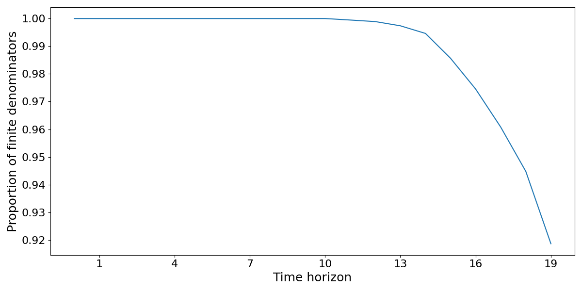
Figure 5: The figure displays the proportion of action trajectory pairs where the associated denominator value for \(\textrm{MASD}_{\textrm{Weight-}t}(k,a_{0:t}',a_{0:t}''){}\) is finite. The \(\textrm{MASD}_{\textrm{Weight-}t}(k,a_{0:t}',a_{0:t}''){}\) values are defined with respect to the sepsis dataset, under the vanilla estimator, with the x-axis displaying the time horizon and y-axis displaying the proportion of finite denominators.. a — Training dataset, b — Testing dataset
Figure 6 displays the median \(\textrm{MASD}_{\textrm{Weight-}t}(k,t){}\) but for the clipped importance sampling estimator ([@ionides_truncated_2008]) and figure 7 displays the median \(\textrm{MASD}_{\textrm{Weight-}t}(k,t){}\) for the Hajek estimator. Both the clipped and Hajek estimators present a similar story to the vanilla estimator. Under the clipped estimator covariate balance cannot be concluded to be
achieved, since the metric values are greater than 0.25. Without a formal analysis, it is unclear whether the 0.25 cut-off proposed by [@cannas_comparison_2019] can be applied to the Hajek
estimator. Under both the clipped and Hajek estimators, similarly to the vanilla estimator, balance appears to improve with horizon. Figures 8 and 9 display the decomposition of \(\textrm{MASD}_{\textrm{Weight-}t}(k,a_{0:t}',a_{0:t}''){}\) by numerator and
denominator (similarly to figure 4). In comparison to the vanilla estimator, the unormalised numerator of the \(\textrm{MASD}_{\textrm{Weight-}t}(k,t){}\) metric does not diverge, suggesting that the apparent improvement in covariate balance under the estimator at longer time horizons can be trusted. However, subsequent analysis (section
4.2.3.1) will demonstrate that this apparent improvement is an artefact of the estimators.


Figure 6: The figure describes the median \(\textrm{MASD}_{\textrm{Weight-}t}(k,t){}\) value using clipped importance sampling, across features on the sepsis dataset. The x-axis displays the time horizon and the y-axis displays the median \(\textrm{MASD}_{\textrm{Weight-}t}(k,t){}\) value as the solid line with the min and max values described by the shaded region. The dotted line is a reference for the value 1.. a — Training dataset, b — Testing dataset


Figure 7: The figure describes the median \(\textrm{MASD}_{\textrm{Weight-}t}(k,t){}\) value using Hajek importance sampling, across features on the sepsis dataset. The x-axis displays the time horizon and the y-axis displays the median \(\textrm{MASD}_{\textrm{Weight-}t}(k,t){}\) value as the solid line with the min and max values described by the shaded region. The dotted line is a reference for the value 1.. a — Training dataset, b — Testing dataset


Figure 8: The figure describes the median numerator and denominator of the \(\textrm{MASD}_{\textrm{Weight-}t}(k,a_{0:t}',a_{0:t}''){}\) metric, across features on the sepsis dataset, under the clipped estimator. The x-axis displays the time horizon. Aggregations are taken over action trajectory pairs with finite denominators.. a — Training dataset, b — Testing dataset


Figure 9: The figure describes the median numerator and denominator of the \(\textrm{MASD}_{\textrm{Weight-}t}(k,a_{0:t}',a_{0:t}''){}\) metric, across features on the sepsis dataset, under the Hajek estimator. The x-axis displays the time horizon. Aggregations are taken over action trajectory pairs with finite denominators.. a — Training dataset, b — Testing dataset
Figures 10, 11 and 12 describe the median (across
features) \(\textrm{MASD-Diff}_{\textrm{Weight-}t}(k,t){}\) values on the sepsis dataset. The blue describes the range of values where covariate balance is improved under the propensity model and orange describes the
opposite. For the vanilla estimator, the result supports the deduction that covariate balance degrades with horizon. In particular, after timepoint 3 on the training set and timepoint 2 on the testing set, the median \(\textrm{MASD-Diff}_{\textrm{Weight-}t}(k,t){}\) across features is not greater than 0. Figure 11, displaying balance under the clipped estimator, suggests the
propensity model improves covariate balance for the entire trajectory. This is similarly the case for the Hajek estimator, presented in figure 12. A conclusion regarding the validity of
this claim is reserved until the bias of the estimator is explored, as already alluded to.


Figure 10: The figure describes the median (across features) \(\textrm{MASD-Diff}_{\textrm{Weight-}t}(k,t){}\) values on the sepsis dataset, under the vanilla estimator. The shaded region describes the min and max \(\textrm{MASD-Diff}_{\textrm{Weight-}t}(k,t){}\) values by timepoint.. a — Training dataset, b — Testing dataset


Figure 11: The figure describes the median (across features) \(\textrm{MASD-Diff}_{\textrm{Weight-}t}(k,t){}\) values on the sepsis dataset, under the clipped estimator. The shaded region describes the min and max \(\textrm{MASD-Diff}_{\textrm{Weight-}t}(k,t){}\) values by timepoint.. a — Training dataset, b — Testing dataset


Figure 12: The figure describes the median (across features) \(\textrm{MASD-Diff}_{\textrm{Weight-}t}(k,t){}\) values on the sepsis dataset, under the Hajek estimator. The shaded region describes the min and max \(\textrm{MASD-Diff}_{\textrm{Weight-}t}(k,t){}\) values by timepoint.. a — Training dataset, b — Testing dataset
4.2.3.1 Bias investigation for clipped and Hajek importance sampling
Figure 13 displays scatter plots of the average (across intervention level) original covariate on the x-axis (i.e., \(g(s_{i,0:t,k})\)) against the
weighted covariate on the y-axis (i.e., \(g(s_{i,0:t,k})(\prod_{t'=0}^{t}p(a_{i,t'}|s_{i,t'}))^{-1}\) from equation 13 ). The fewer points observed at timestep 1 is a
function of the fact that the number of potential interventions increases as \(25^{t+1}\). Across the timesteps, a non-zero amount of variance is retained by the map from the unweighted to the weighted covariate (i.e.,
between the x and y axes).
Figures 14 and 15 display the same information as figure 13 but for the clipped and Hajek estimators, respectively. Visually, in comparison to the vanilla estimator, the variance in the importance weighted projection of the covariates vanishes
at longer time horizons. Let \(h(s_{i,t,k})\) define the projected covariate under an importance weighting regimen i.e.: \[\begin{align} h_{\textrm{Vanilla}}(s_{i,t,k},a_{0:t}) =&
\frac{g(s_{i,0:t,k})}{\prod_{t'=0}^{t}p(a_{i,t'}|s_{i,t'})}\\ h_{\textrm{Clipped}}(s_{i,t,k},a_{0:t}) =& \frac{g(s_{i,0:t,k})}{\zeta \vee \prod_{t'=0}^{t}p(a_{i,t'}|s_{i,t'})}\\ h_{\textrm{Hajek}}(s_{i,t,k},a_{0:t}) =&
\frac{g(s_{i,0:t,k})}{\prod_{t'=0}^{t}p(a_{i,t'}|s_{i,t'})(\sum \prod_{t'=0}^{t}p(a_{i,t'}|s_{i,t'}))^{-1}}
\end{align}\] The lack of variance for a given value of \(g(s_{i,0:t,k})\) under the \(h_{\textrm{Clipped}}\) and \(h_{\textrm{Hajek}}\) projections
(demonstrated by figures 14 and 15) implies \(h_{\textrm{Clipped}}(s_{i,t,k},a_{0:t}) = h_{\textrm{Clipped}}(s_{i,t,k},a_{0:t}')\) and \(h_{\textrm{Hajek}}(s_{i,t,k},a_{0:t}) = h_{\textrm{Hajek}}(s_{i,t,k},a_{0:t}')\) i.e., the bias
introduced by the clipped and Hajek estimators results in the covariate projections collapsing to a single value for a given covariate value, \(g(s_{i,0:t,k})\) and for all intervention levels, \(a_{0:t}\). The implication is that, under high variance regimens (e.g., long time horizons), the covariate weight under the clipped and Hajek estimators will be equal for all actions trajectories, giving the impression of
balance that is equivalent to the unweighted state i.e., does not degrade but does not improve. Recall, figures 11 and 12 demonstrated that the \(\textrm{MASD-Diff}_{\textrm{Weight-}t}(k,t){}\) values converged to 0 with time and thus maybe a function of the afore described
phenomena.


Figure 13: The figure displays scatter plots of the average (across intervention level) covariate value on the x-axis against the weighted covariate (i.e., \(g(s_{i,0:t,k})(\prod_{t'=0}^{t}p(a_{i,t'}|s_{i,t'}))^{-1}\) from equation 13 ) on the y-axis. The weighted covariate values are clipped between the 10th and 90th percentile of the original distribution. The figure displays timestep 1 at the top, timestep 4 in the middle and timestep 16 at the bottom, with propensity score predictions made over seed 0 of the training dataset.. a — Timestep 1, b — Timestep 4, c — Timestep 16


Figure 14: The figure displays scatter plots of the average (across intervention level) covariate value on the x-axis against the clipped importance weighted covariate (i.e., \(g(s_{i,0:t,k})(\prod_{t'=0}^{t}p(a_{i,t'}|s_{i,t'}))^{-1}\) from equation 13 ) on the y-axis. The weighted covariate values are further clipped between the 10th and 90th percentile of the original distribution. The figure displays timestep 1 at the top, timestep 4 in the middle and timestep 16 at the bottom, with propensity score predictions made over seed 0 of the training dataset.. a — Timestep 1, b — Timestep 4, c — Timestep 16


Figure 15: The figure displays scatter plots of the average (across intervention level) covariate value on the x-axis against the Hajek importance weighted covariate (i.e., \(g(s_{i,0:t,k})(\prod_{t'=0}^{t}p(a_{i,t'}|s_{i,t'}))^{-1}\) from equation 13 ) on the y-axis. The weighted covariate values are clipped between the 10th and 90th percentile of the original distribution. The figure displays timestep 1 at the top, timestep 4 in the middle and timestep 16 at the bottom, with propensity score predictions made over seed 0 of the training dataset.. a — Timestep 1, b — Timestep 4, c — Timestep 16
4.2.3.2 Bias analysis of clipped importance sampling
Let: \[\begin{align} d=\{\tau_{i}\}_{i=1}^{n}=\{s_{i,0},a_{i,0},...,s_{i,H-2},a_{i,H-2},s_{i,H-1}\}_{i=1}^{n} \end{align}\] with density defined by equation 12 . For a sufficiently large time horizon, \(t\), since \(p(a_{i,t'}|s_{i,t'})\) is a normalised probability density, observe that \(\forall \tau\in d, \prod_{t'=0}^{H-2}p(a_{i,t'}|s_{i,t'}) \vee \zeta = \zeta\). Then: \[\begin{align} \hat{\mu}_{a_{0:t}'}(k) = & \frac{1}{n}\sum_{i=1}^{n}\frac{\mathbb{1}(a_{i,0:t}=a_{0:t}')g(s_{i,0:t,k})}{\zeta} \\ =& \zeta^{-1}\Bigg(\frac{1}{n}\sum_{i=1}^{n}\mathbb{1}(a_{i,0:t}=a_{0:t}')g(s_{i,0:t,k})\Bigg) \end{align}\] Additionally, for simplicity, considering the biased estimate of \(\sigma^{2}_{a_{0:t}'}(k)\): \[\begin{align} \bar{\sigma}^{2}_{a_{0:t}'}(k) =& \frac{1}{n}\sum_{i=1}^{n}\Bigg(\frac{\mathbb{1}(a_{i,0:t}=a_{0:t}')g(s_{i,0:t,k})}{\prod_{t'=0}^{t}p(a_{i,t'}|s_{i,t'})} - \hat{\mu}_{a_{0:t}'}\Bigg)^{2} \\ =& \frac{1}{n}\sum_{i=1}^{n}\Bigg(\frac{\mathbb{1}(a_{i,0:t}=a_{0:t}')g(s_{i,0:t,k})}{\prod_{t'=0}^{t}p(a_{i,t'}|s_{i,t'})}\Bigg)^{2}\\ & - \Bigg(\frac{1}{n}\sum_{i=1}^{n}\frac{\mathbb{1}(a_{i,0:t}=a_{0:t}')g(s_{i,0:t,k})}{\prod_{t'=0}^{t}p(a_{i,t'}|s_{i,t'})}\Bigg)^{2} \\ =& \frac{1}{n}\sum_{i=1}^{n}\Bigg(\frac{\mathbb{1}(a_{i,0:t}=a_{0:t}')g(s_{i,0:t,k})}{\zeta}\Bigg)^{2}\\ & - \Bigg(\frac{1}{n}\sum_{i=1}^{n}\frac{\mathbb{1}(a_{i,0:t}=a_{0:t}')g(s_{i,0:t,k})}{\zeta}\Bigg)^{2} \\ =& \zeta^{-2}\Bigg(\frac{1}{n}\sum_{i=1}^{n}\bigg(\mathbb{1}(a_{i,0:t}=a_{0:t}')g(s_{i,0:t,k})\bigg)^{2}\\ &- \Bigg(\frac{1}{n}\sum_{i=1}^{n}\mathbb{1}(a_{i,0:t}=a_{0:t}')g(s_{i,0:t,k})\Bigg)^{2}\Bigg) \end{align}\]
Combining the numerator and denominator, observe that: \[\begin{align} \frac{|\hat{\mu}_{a_{0:t}'}(k)-\hat{\mu}_{a_{0:t}''}(k)|}{\sqrt{n^{-1}\bar{\sigma}^{2}_{a_{0:t}'}(k) +
n^{-1}\bar{\sigma}^{2}_{a_{0:t}''}(k)}} = \frac{\zeta^{-1}|\hat{\mu\prime}_{a_{0:t}'}(k)-\hat{\mu\prime}_{a_{0:t}''}(k)|}{\sqrt{\zeta^{-2}(n^{-1}\bar{\sigma\prime}^{2}_{a_{0:t}'}(k) +
n^{-1}\bar{\sigma\prime}^{2}_{a_{0:t}''}(k))}} \\
\end{align}\] where \(\hat{\mu\prime}_{a_{0:t}'}(k)\) and \(\bar{\sigma\prime}^{2}_{a_{0:t}'}(k)\) are the unweighted mean and standard deviation. Which implies, for a
sufficiently large \(t\): \[\label{equ:masd95propto95large95t} \textrm{MASD}_{\textrm{Weight-}t}(k,a_{0:t}',a_{0:t}''){} \approx
\textrm{MASD}_{\textrm{UnWeight-}t}(k,a_{0:t},a_{0:t}'')\tag{15}\] Equation 15 explains the apparent positive covariate balance observed when considering the clipped importance sampling
estimator, demonstrated in figures 6 and 11.
4.2.3.3 Bias analysis of Hajek importance sampling
A similar deduction regarding the bias of the Hajek estimator can be made. However, unlike the clipping estimator, the resulting bias is driven by the exponential reduction in effective sample size. This is demonstrated in figure 16, displaying the number of observations per intervention level, split by time for the training and testing datasets.


Figure 16: The figure displays the aggregate number of observations per intervention level, across time. The thick blue line defines the mean number of observations whilst the shaded area defines and min and max.. a — Training set, b — Testing set
Returning to the Hajek estimator, \(\textrm{MASD}_{\textrm{Hajek-}t}(k,a_{0:t}',a_{0:t}''){}\), for a sufficiently large \(t\): \[\begin{align} \frac{\frac{\mathbb{1}(a_{i,0:t}=a_{0:t}')g(s_{i,0:t,k})}{\prod_{t'=0}^{t}p(a_{i,t'}|s_{i,t'})}}{\frac{1}{n}\sum_{i=1}^{n}\frac{\mathbb{1}(a_{i,0:t}=a_{0:t}')}{\prod_{t'=0}^{t}p(a_{i,t'}|s_{i,t'})}} = \mathbb{1}(a_{i,0:t}=a_{0:t}')g(s_{i,0:t,k})\\ \end{align}\] As such: \[\begin{align} \frac{\frac{1}{n}\sum_{i=1}^{n}\frac{\mathbb{1}(a_{i,0:t}=a_{0:t}')g(s_{i,0:t,k})}{\prod_{t'=0}^{t}p(a_{i,t'}|s_{i,t'})}}{\frac{1}{n}\sum_{i=1}^{n}\frac{\mathbb{1}(a_{i,0:t}=a_{0:t}')}{\prod_{t'=0}^{t}p(a_{i,t'}|s_{i,t'})}} = \frac{1}{n}\sum_{i=1}^{n}\mathbb{1}(a_{i,0:t}=a_{0:t}')g(s_{i,0:t,k}) \end{align}\] and: \[\begin{align} & \frac{1}{n-1}\sum_{i=1}^{n}\Bigg(\frac{\frac{\mathbb{1}(a_{i,0:t}=a_{0:t}')g(s_{i,0:t,k})}{\prod_{t'=0}^{t}p(a_{i,t'}|s_{i,t'})}}{\frac{1}{n}\sum_{i=1}^{n}\frac{\mathbb{1}(a_{i,0:t}=a_{0:t}')}{\prod_{t'=0}^{t}p(a_{i,t'}|s_{i,t'})}} - \hat{\mu}_{a_{0:t}'}\Bigg)^{2} \\ & = \frac{1}{n-1}\sum_{i=1}^{n}\Bigg(\mathbb{1}(a_{i,0:t}=a_{0:t}')g(s_{i,0:t,k}) - \frac{1}{n}\sum_{i=1}^{n}\mathbb{1}(a_{i,0:t}=a_{0:t}')g(s_{i,0:t,k})\Bigg)^{2} \end{align}\] Thus, similarly to the clipped estimator, for a sufficiently large \(t\): \[\begin{align} \textrm{MASD}_{\textrm{Hajek-}t}(k,a_{0:t}',a_{0:t}''){} \approx \textrm{MASD}_{\textrm{UnWeight-}t}(k,a_{0:t},a_{0:t}'') \end{align}\]
4.2.3.4 Summary
To conclude, the high variance of the importance sampling estimator precludes drawing a conclusion regarding the presence of covariate balance at later timesteps. Furthermore, controlling this variance using the conventional clipping and weighting
arguably worsens the issue since both methods bias towards perfect covariate balance in high variance settings. More encouragingly, both the clipped and Hajek estimators did suggest covariate balance was present beyond the first three timesteps where, from
figures 14 and 15, there is still variation in the weighted states. This argument however, is
entirely heuristic and a formal framework describing the trade-off between accuracy and variance reduction would be extremely useful. Pessimistic PAC based estimators for clipped importance sampling have been widely established ([@sakhi2024logarithmic]) and thus would provide a solid starting point for developing such a framework. An immediate and potentially significant challenge in adapting these estimators however, is the desirability of
pessimism in the context of covariate balance.
4.2.4 Fluid action space (Sepsis-fluid dataset)↩︎
Under the full action space used in the previous section, a number of actions were drastically underrepresented even before accounting for the cumulative effect over time. Figures 22 and 23 describe the proportion of observations split by action over time. At a high level, for the sepsis dataset, the minimum representation for a given action was only 3% of the total observations
(calculated using the seed 0 training set). It was hypothesised that this lead to higher variance in the covariate balance metrics due to the reduced effective sample size, as demonstrated by figure 17 (a). This is in contrast to figure 17 (b) where the effective sample size of a given intervention reduces to 0 at a
later time horizon (judging by the minimum value).

Figure 17: The figures describe the mean (blue solid line) and min/max (shaded area) number of observations per intervention level, across time. The seed 0 training set was used to produce the figures.. a — Sepsis dataset, b — Sepsis-fluid dataset
Figures 18 and 19 display the median \(\textrm{MASD}_{\textrm{Weight-}t}(k,t){}\) and \(\textrm{MASD-Diff}_{\textrm{Weight-}t}(k,t){}\) values for the sepsis-fluid dataset, respectively. In comparison to the sepsis datasets, the
propensity model induces better covariate balance for the first four timesteps (on the testing dataset) instead of the first two (figure 19). However, using the restricted
action space far from resolves the lack of covariate balance: balance worsens from timestep 4 onwards in comparison to the unweighted covariates.
The predictive performance of the propensity score also improved under the sepsis-fluid dataset (table 1) which was almost certainly a result of the more uniform action density. Since the propensity model needs to
be correctly specified to achieve covariate balance (corollary 2), this improvement in performance is a confounder for
understanding the impact of the reduced action space. Subsequent analysis in section 5.1 demonstrates that sample size does indeed impact covariate balance. As such, all that is unknown is the extent to
which the relative balance between the sepsis and the sepsis-fluid datasets is mediated by the improvement in the propensity model performance.


Figure 18: The figure describes the median \(\textrm{MASD}_{\textrm{Weight-}t}(k,t){}\) value, across features, for the sepsis-fluid dataset, under the vanilla estimator. The x-axis displays the time horizon and the y-axis displays the median \(\textrm{MASD}_{\textrm{Weight-}t}(k,t){}\) value as the solid line with the min and max values described by the shaded region.. a — Training dataset, b — Testing dataset


Figure 19: The figure describes the median (across features) \(\textrm{MASD-Diff}_{\textrm{Weight-}t}(k,t){}\) values for the sepsis-fluid dataset, under the vanilla estimator. The shaded region describes the min and max \(\textrm{MASD-Diff}_{\textrm{Weight-}t}(k,t){}\) values by timepoint.. a — Training dataset, b — Testing dataset


Figure 20: The figure describes the median (across features) \(\textrm{MASD-Diff}_{\textrm{Weight-}t}(k,t){}\) values for the sepsis-fluid dataset, under the clipped estimator. The shaded region describes the min and max \(\textrm{MASD-Diff}_{\textrm{Weight-}t}(k,t){}\) values by timepoint.. a — Training dataset, b — Testing dataset


Figure 21: The figure describes the median (across features) \(\textrm{MASD-Diff}_{\textrm{Weight-}t}(k,t){}\) values for the sepsis-fluid dataset, under the Hajek estimator. The shaded region describes the min and max \(\textrm{MASD-Diff}_{\textrm{Weight-}t}(k,t){}\) values by timepoint.. a — Training dataset, b — Testing dataset


Figure 22: The figure describes the proportion of actions per timestep, across the training and testing sets, and split by seeds for the sepsis dataset.. a — Training dataset (seed 0), b — Testing dataset (seed 0), c — Training dataset (seed 1), d — Testing dataset (seed 1)


Figure 23: The figure describes the proportion of actions per timestep, across the training and testing sets, and split by seeds for the sepsis-fluid dataset.. a — Training dataset (seed 0), b — Testing dataset (seed 0), c — Training dataset (seed 1), d — Testing dataset (seed 1)
4.2.5 Reduced time horizon↩︎
The results presented in sections 4.2.3 and 4.2.4 have suggested that covariate balance might be present over a shorter time horizon. Similar to constraining
the action space, as discussed in section 4.2.4, constraining the planning horizon might provide a reasonable approach to ensuring covariate balance is satisfied. This hypothesis was assessed by evaluating
covariate balance for propensity models trained on horizons of length 2, 5, 8 and 13 timesteps. Horizons 5 and 13 were chosen since these defined the 5th and 50th percentile of trajectory lengths, calculated on the training set under seed 0. Horizon 2 was
chosen as this defines the minimum multistep horizon. Horizon 8 was subsequently included based on the results of 5 and 13. Table 2 displays the number of timesteps where the median \(\textrm{MASD-Diff}_{\textrm{Weight-}t}(k,t){}>0\) and appendix section [sec:reduced_time_horizon_appendix] contains the complete median (across features) \(\textrm{MASD}_{\textrm{Weight-}t}(k,t){}\) and \(\textrm{MASD-Diff}_{\textrm{Weight-}t}(k,t){}\) plots.
| Dataset | Horizon | # median \(\masdtdiffmean{}>0\) | |
| Training | Testing | ||
| Sepsis | 2 | 2 | 2 |
| Sepsis | 5 | 3 | 2 |
| Sepsis | 8 | 3 | 3 |
| Sepsis | 13 | 3 | 2 |
| Sepsis-fluid | 2 | 2 | 2 |
| Sepsis-fluid | 5 | 5 | 5 |
| Sepsis-fluid | 8 | 5 | 4 |
| Sepsis-fluid | 13 | 5 | 4 |
The results in table 2 demonstrate that, across the sepsis and sepsis-fluid datasets, reducing the time horizon can improve the resulting covariate balance, albeit this is not uniformly the case. Of
the restricted trajectory lengths assessed, covariate balance never worsened and improved on the sepsis dataset at horizon 8 and on the sepsis fluid dataset at horizon 5.
For all restricted time horizons and across both action spaces, the action dimension was effectively the same as under the original time horizon. There was a risk that certain actions were only present in later timesteps of the trajectories and thus by
considering truncated trajectories, the action space would also effectively be reduced. Since it had already been demonstrated that a reduced action space dimension improved covariate balance (section 4.2.4),
reducing the action space along with the horizon risked confounding the analysis. However, as stated the action space dimension was identical except for the first timestep under the sepsis dataset where the effective action dimension was 24 rather than 25.
Since the action dimension was effectively retained, any improvement in covariate balance could reasonably be attributed to truncating the trajectories.
Since covariate balance did not uniformly improve across all truncated horizons (or uniformly across all horizons below a given length), further assessment is required, to ensure these results were not statistical anomalies. It is perhaps counterintuitive
that restricting the maximum time horizon would increase the horizon over which covariate balance is present. It is hypothesised however, that truncating the horizon improves the stability of training the propensity model. This is discussed further in
section 5.2.
5 Conclusion↩︎
The core implication of the analysis is that existing applications of offline reinforcement learning for learning treatment recommendations are too high dimensional (both in time and action space) to conclude, using existing approaches for assessing
diagnostic balance that, at least heuristically, conditional exchangeability holds. With respect to the sepsis domain assessed, figures 10 and 19 combined suggest that covariate balance can be achieved for the first 2 timesteps and this can be improved by restricting the action space and potentially by truncating
trajectories.
A second implication of the analysis is that, traditional approaches to reducing variance in importance sampling estimators are not valid for assessing covariate balance. As the variance of the vanilla estimator (and thus uncertainty) increases, both the
Hajek and clipped estimator will predictably suggest that covariate balance has been achieved. Arguably, it is unsurprising that the clipped and Hajek estimators are insufficient for assessing covariate balance. Where sequential exchangeability does not
hold, the resulting causal estimates are biased. As a result, the MASD metrics are a diagnostic check for bias. On the surface, checking for bias using biased estimators (without proper control) feels counterintuitive. An impactful line of future work
would consider the point at which the bias under the clipped or Hajek estimators overwhelms the estimates. If this could be characterised, then far greater confidence could be placed in the presence of covariate balance at timesteps larger than 2, for the
sepsis dataset assessed in this analysis (based on figures 11 and 12).
5.1 Training/validation set↩︎
As discussed in section 4.1, it is intuitive to consider the covariate balance over the training set to be a biased estimate of the expected covariate balance. On the surface, the general degradation in
balance between the testing and training set supports this. Figure 24 describes the median (across features) \(\textrm{MASD-Diff}_{\textrm{Weight-}t}(k,t){}\) values, calculated on seed 0 of the training data but subsampled to be the size of the testing set, for the sepsis and sepsis-fluid datasets, respectively. Notably, in comparison
to figure 10 for the sepsis dataset and 19 for the sepsis-fluid datasets, the number of timesteps with a
positive median covariate balance is equivalent to that observed on the testing sets. It is thus quite possible that the degradation in balance on the testing set is a function of the reduced sample size, rather than the training set metric being
inherently biased/the bias being substantial.


Figure 24: The figure describes the median (across features) \(\textrm{MASD-Diff}_{\textrm{Weight-}t}(k,t){}\) values for seed 0 of the training data, subsampled to the size of the testing set. The metric values are derived under the vanilla importance sampling estimator. The shaded region describes the min and max \(\textrm{MASD-Diff}_{\textrm{Weight-}t}(k,t){}\) values by timepoint.. a — Sepsis dataset, b — Sepsis-fluid dataset
Without considering the use of covariate balance for model training (in the case of [@Imai2014]), it is quite possible that the bias (if any) from assessing covariate balance on the training set (or
even better the joint training and testing set) is sufficiently small such that the increased sample size provides a more accurate view of the covariate balance achieved. Given this observation, an important line of future work would be to establish the
behaviour of covariate balance to determine whether the training set can be used to assess balance.
5.2 Propensity score architecture↩︎
The derivation of the weighted MASD metrics described in section 3.3 utilised the independence structure of the MDP to simplify the time \(t\) propensity estimate
by equating \(p(A_{0:t}|S_{0:t})=\prod_{t'=0}^{t}p(A_{t'}|S_{t'})\). This autoregressive approach is common for sequence modelling. An alternate modelling approach would be to jointly learn the density of the
trajectory. The results presented in 4.2.5 potentially support the hypothesis that this joint modelling approach would benefit the development of propensity models. The results showed that by truncating the
trajectory length, the number of timesteps where covariate balance was present (relative to the unweighted distribution) improved, in some scenarios. It was hypothesised that this was a result of the global structure of the trajectory being easier to
capture.
The causal structure of the MDP would still need to be respected and thus the marginal decomposition would still exist however, a joint modelling approach might improve the overall stability of the inferred densities at later time horizons. It is
hypothesised that such an approach might trade-off a degraded covariate stability earlier in trajectories for an improved covariate stability at later timesteps.
More concretely, the current training process learnt \(p(A_{t}|S_{t},A_{t-1})\). The joint density was subsequently defined by \(p(A_{0:t}|S_{0:t},A_{0:t-1})=
p(A_{0}|S_{0})\prod_{t'=1}^{t}p(A_{t}|S_{t},A_{t-1})\). A joint modelling approach would learn \(p(A_{0:H-1}|S_{0:H-1},A_{0:H-2})\) directly and thus \(p(A_{0:t}|S_{0:t},A_{0:t-1}) =
\int p(A_{0:H-1}|S_{0:H-1},A_{0:H-2}) dA_{t+1:H-1},S_{t+1:H-1}\).