Fully discrete least-squares splitting scheme for the Monge-Ampère equation: finite element analysis and convergence
July 16, 2026
Abstract
The least-squares splitting algorithm for the Monge-Ampère equation has been used successfully in computations for several years, but a convergence theory for fully discrete splitting schemes of this type has remained unavailable. In this work, we introduce and analyze a finite element framework for smooth solutions of the Dirichlet Monge-Ampère equation in two dimensions. The proposed schemes combine a discrete Hessian reconstruction with a local projection onto the determinant constraint. Under a discrete Miranda-Talenti estimate and standard approximation properties of the Hessian reconstruction, we prove local convergence of the iterative scheme and optimal-order convergence of its limit to the exact solution in an \(H^2\)-type norm. We verify the estimates for conforming \(C^1\) schemes, including the Argyris element, and for \(C^0\)-interior penalty and DG schemes of degree at least three; quadratic \(C^0\)-interior penalty and DG schemes are also covered when \(|u|_{H^3(\Omega)}\) is sufficiently small. To the best of our knowledge, these discretizations have not previously been proposed or analyzed for least-squares splitting methods. Numerical experiments confirm the theoretical convergence rates.
1 Introduction↩︎
Fully nonlinear second-order partial differential equations arise in a wide range of applications, including differential geometry, optimal transport, geometric optics, meteorology, and stochastic control [1], [2]. Among them, the Monge-Ampère equation is one of the prototypical examples. In its elliptic Dirichlet form, on a bounded convex domain \(\Omega\subset \mathbb{R}^2\), it reads as \[\det D^2 u = f \quad \text{in } \Omega, \qquad u=g \quad \text{on } \partial\Omega,\] where the admissible solution is required to be convex. This convexity requirement selects the elliptic branch of the equation and is essential for uniqueness [1], [3].
The analysis of fully nonlinear equations is substantially more delicate than that of linear or semilinear elliptic problems. Even for smooth data, classical regularity may require additional structural assumptions on the domain, the boundary data, and the solution itself, see [1], [3]. From the numerical point of view, several difficulties arise. First, fully nonlinear second-order equations do not generally admit a standard weak formulation obtained by integration by parts. Consequently, methods aimed at approximating smooth solutions must either work directly with Hessians, and therefore with an \(H^2\)-type structure, or introduce suitable discrete Hessians, stabilizations, or auxiliary variables. Second, the nonlinearity has to be handled in a robust way at the discrete level. Third, for equations such as Monge-Ampère, uniqueness is tied to the correct admissible class, namely the class of convex functions.
Nonetheless, over the last decades, several Galerkin-based methods have been developed for smooth solutions of the Dirichlet Monge-Ampère problem. These include vanishing moment methods [4], mixed finite element methods [5], [6], \(C^1\) finite element methods [7]–[9], \(C^0\)-interior penalty methods [10], [11], discontinuous Galerkin methods [12], and least-squares formulations [13]–[15]; see also the surveys [2], [16]. The present work focuses on the nonlinear least-squares splitting method introduced by Dean and Glowinski [17] and subsequently developed in [18]–[20]. This method introduces an auxiliary matrix variable \(\mathbf{P}\), interpreted as an approximation of \(D^2u\), and rewrites the Monge-Ampère equation as the constrained problem \[\mathbf{P} = D^2u\,\text{ in }\Omega, \qquad \det \mathbf{P} = f\,\text{ in }\Omega, \qquad u = g \,\text{ on }\partial\Omega.\] The corresponding least-squares formulation, defined in 2, looks for the minimizers of the \(L^2\) distance between the set of admissible Hessians and the nonlinear constraint set. The resulting splitting algorithm alternates between a linear variational problem and a pointwise nearest-point projection [17], [18], [21]. Its computational efficiency stems from the fact that the nonlinear subproblem is local, while the differential subproblem remains linear.
The method has shown good numerical performance, especially in low-order \(C^0\) implementations [18], [20], where the differential subproblem can be reduced to the solution of Poisson-type problems. It has also been extended to optimal transport and optics problems [22], [23], as well as to other classes of fully nonlinear PDEs [24]–[26]. However, despite this numerical evidence, a rigorous convergence analysis of the fully discrete splitting iteration has not been made available. A recent analysis in the continuous setting reinterprets the method as an alternating projection algorithm in Sobolev spaces and proves convergence at the continuous level on \(\mathbb{T}^2\); see [27]. The present work develops a unified framework for the corresponding fully discrete convergence analysis on general bounded convex polygonal domains. We prove that, under suitable assumptions on the discretization of the linear variational subproblem, the iterative method converges locally and its limit converges to the exact solution in an \(H^2\)-type norm at optimal rate with respect to the mesh size. We further verify these assumptions for representative \(C^1\), \(C^0\) and DG finite element methods.
1.1 Related works↩︎
There are (at least) two ways to organize the existing literature on Galerkin-type methods for the Monge-Ampère equation. One may classify methods according to the discrete space used, for instance \(C^1\), \(C^0\)-interior penalty, discontinuous Galerkin, or mixed finite element spaces. Alternatively, one may classify them according to the nonlinear strategy used to solve the discrete problem, for instance Newton’s method, time-marching methods, fixed-point iterations, or least-squares splitting methods.
A substantial part of the finite element literature relies on Newton-type linearizations. For instance, local well-posedness and convergence estimates for discrete Monge-Ampère problems have been obtained for \(C^1\), \(C^0\)-interior penalty, discontinuous Galerkin, and mixed finite element methods [6], [7], [10], [12]. The convergence of Newton’s method for such discretizations has also been studied, for example, in [6], [28]. These results are local: the discrete solution is constructed, and the nonlinear iteration is shown to converge, under the assumption that the initial guess belongs to a mesh-dependent neighbourhood of the exact discrete solution.
Newton’s method is not the only possible iterative strategy. [11] proposed a time-marching method based on \(C^0\) finite elements, using an explicit Euler discretization of the evolution equation \(\partial_t(\Delta u)=\det D^2u - f\). As with Newton’s method, convergence is again proved in a local neighborhood whose radius depends on the mesh size. Mesh-dependent local neighbourhoods also appear in the analysis of the vanishing moment method [4], [29], [30], where the relevant fixed-point argument is carried out for the \(\varepsilon\)-regularized fourth-order problem.
The fact that the convergence neighbourhood shrinks with the mesh size is closely related to the need to control the discrete Hessian in a pointwise norm, as also highlighted in [27]. Since the nonlinear operator depends on \(D^2u\), one needs to ensure that the discrete Hessian remains in the correct elliptic regime. At the discrete level, such a pointwise control is usually obtained from an inverse estimate, which converts an \(H^2\)-type bound into a \(W^{2,\infty}\)-type bound at the cost of a negative power of \(h\). This mechanism is also present in the analysis developed below.
1.2 Contribution↩︎
The main contribution of this work is the first local convergence theory for fully discrete least-squares splitting schemes for the Dirichlet Monge-Ampère equation, showing that these methods admit the same type of local convergence guarantees as more classical nonlinear iterative methods. We formulate the method in an abstract finite element framework, in terms of a discrete Hessian reconstruction \(H_h\), a stabilization bilinear form \(J_h\), and a pointwise metric projection onto the determinant constraint. This setting includes conforming \(C^1\), \(C^0\)-interior penalty, and discontinuous Galerkin discretizations. To the best of our knowledge, these discretizations have not previously been combined with the Dean-Glowinski least-squares splitting strategy.
Following the continuous analysis in [27], we interpret the least-squares splitting algorithm as a discrete alternating minimization method. The convergence analysis relies on two assumptions on the reconstruction step: a discrete Miranda-Talenti stability estimate and a consistency estimate for the discrete Hessian reconstruction. Under these assumptions, we prove in 2 that the fully discrete alternating minimization map is a strict contraction in a mesh-dependent neighbourhood of the exact solution. This yields the existence of a locally unique discrete fixed point and convergence of the iteration. The key estimate, 2, is a discrete transversality bound between the linear reconstruction step and the tangent space to the determinant constraint. We then verify the abstract assumptions for conforming \(C^1\), including the Argyris element, and for \(C^0\)-interior penalty, and DG discretizations of polynomial degree at least three. Quadratic \(C^0\)-interior penalty and DG discretizations are also covered provided that the \(H^3\)-seminorm of the exact solution is sufficiently small, see 3. 2 also yields the reconstructed Hessian error estimates stated in [cor:conv_c1,cor:conv_c0,cor:convdg].
For the original low-order realizations of [18], [20], the main remaining obstacle is an appropriate discrete Miranda-Talenti estimate; the same framework may also be applied to other existing or future low-order reconstructions once the required stability and consistency properties are proven. Finally, as discussed in 4, the method could extend to other smooth uniformly elliptic fully nonlinear operators.
1.3 Outline↩︎
The remainder of this work is organized as follows. 2 introduces the continuous least-squares formulation and splitting algorithm for the Monge-Ampère equation. 3 presents the abstract fully discrete framework, while 4 establishes its convergence. In 5, we verify the assumptions for \(C^1\), \(C^0\)-interior penalty, and discontinuous Galerkin finite element methods. Numerical results are presented in 6.
2 Problem setting and algorithm↩︎
2.1 Notation.↩︎
Henceforth, for an open set \(\Omega\subset \mathbb{R}^2\), we denote by \(H^s(\Omega)\) and \(W^{s,p}(\Omega)\), \(s\ge 0\), \(1\le p\le\infty\), the standard Sobolev spaces, equipped with their usual norms and seminorms. Vector and matrix-valued versions are understood componentwise.
Let \(n\in\mathbb{N}\). Matrices in \(\mathbb{R}^{n\times n}\) are denoted by capital letters, e.g. \(A\), while matrix fields on \(\Omega\) are denoted by bold capital letters, e.g. \(\mathbf{A}\). We write \(\mathbb{S}^n\subset\mathbb{R}^{n\times n}\) for the subspace of symmetric matrices and \(\mathbb{S}^n_{++}\) for the subset of symmetric positive definite matrices. For \(A,B\in\mathbb{R}^{n\times n}\), we use the Frobenius product \(A:B := \operatorname{tr}(A^\top B)\), and the associated Frobenius norm \(|A| := \sqrt{A:A}\). We denote by \(L^2(\Omega;\mathbb{R}^{n\times n})\) the space of square-integrable matrix fields, equipped with the norm \[\|\mathbf{A}\|_{L^2(\Omega)}^2 := \int_\Omega |\mathbf{A}(x)|^2\,dx.\] Given a subset \(M\subset L^2(\Omega;\mathbb{R}^{n\times n})\), we denote by \(\Pi_M\) the metric projection onto \(M\) with respect to this \(L^2\)-inner product.
From now on, let \(\Omega\subset\mathbb{R}^2\) be a convex polygonal domain, and let \(\mathcal{T}_h\) be a shape-regular, quasi-uniform triangulation of \(\Omega\). For \(K\in\mathcal{T}_h\), we set \(h_K:=\operatorname{diam}(K)\) and \(h:=\max_{K\in\mathcal{T}_h}h_K\). For \(r\in\mathbb{N}_0\), we define the broken Sobolev space \[H^r(\mathcal{T}_h) := \bigl\{v\in L^2(\Omega): v|_K\in H^r(K) \;\text{for all } K\in\mathcal{T}_h\bigr\},\] equipped with the norm \[\label{eq:brokennorm} \|v\|_{H^r(\mathcal{T}_h)}^2 := \sum_{K\in\mathcal{T}_h}\|v\|_{H^r(K)}^2.\tag{1}\] Similarly, we set \[\|v\|_{L^\infty(\mathcal{T}_h)} := \max_{K\in\mathcal{T}_h}\|v\|_{L^\infty(K)}.\] Let \(m\ge 0\) be fixed. We define the broken polynomial space \[\label{eq:broken95pol} Z_h := \bigl\{v_h\in L^2(\Omega): v_h|_K\in\mathbb{P}_m(K) \;\text{for all } K\in\mathcal{T}_h\bigr\}.\tag{2}\] Elements of \(Z_h\) are identified with their elementwise polynomial representatives. In particular, restrictions and point values are always understood locally on each element. In the present work, we use a nodal norm. For every \(K\in\mathcal{T}_h\), let \(\{x_{K,j}\}_{j=1}^{N_m}\) be the local nodes obtained from a fixed unisolvent nodal configuration on the reference triangle by affine transformation, where \(N_m=\dim\mathbb{P}_m(K)\). The nodes are understood locally: if two neighbouring elements share the same physical node, the corresponding local degrees of freedom are still treated as distinct. Thus, for \(v_h\in Z_h\), we write \(v_h(x_{K,j}) := (v_h|_K)(x_{K,j})\). We associate with these nodes positive weights \(w_{K,j}\) satisfying \(w_{K,j}\simeq h_K^2\) uniformly with respect to \(K\), \(j\), and \(h\). For example, if \(m=1\), one may take the vertices of \(K\) and set \(w_{K,j}=|K|/3\); alternative choices are considered in 6. We then define the nodal scalar product \[(v_h,z_h)_h := \sum_{K\in\mathcal{T}_h}\sum_{j=1}^{N_m} w_{K,j}v_h(x_{K,j})z_h(x_{K,j}), \qquad v_h,z_h\in Z_h.\] The associated norm is defined by \(\|v_h\|_h^2 := (v_h,v_h)_h\). Similarly, we define \[\|v_h\|_{h,\infty} := \max_{K\in\mathcal{T}_h} \max_{1\le j\le N_m} |v_h(x_{K,j})|, \qquad v_h\in Z_h.\] We shall use the same notation for any piecewise function whose values at the local nodes \(x_{K,j}\) are well defined. On \(Z_h\), the norms \(\|\cdot\|_h\) and \(\|\cdot\|_{h,\infty}\) are equivalent to \(\|\cdot\|_{L^2(\mathcal{T}_h)}\) and \(\|\cdot\|_{L^\infty(\mathcal{T}_h)}\), respectively, with constants independent of \(h\). Moreover, \[\label{eq:inverseest} \|v_h\|_{h,\infty} \le C_{\mathrm{inv}} h^{-1}\|v_h\|_h, \qquad \forall v_h\in Z_h,\tag{3}\] where \(C_{\mathrm{inv}}>0\) is independent of \(h\), see for instance [31]. The definitions of \(H^r(\mathcal{T}_h)\), \(Z_h\), \(\|\cdot\|_{H^r(\mathcal{T}_h)}\), \(\|\cdot\|_h\), and \(\|\cdot\|_{h,\infty}\) extend componentwise to vector-valued and matrix-valued spaces, using the same local nodes and the Euclidean or Frobenius norm at each node. In particular, \(Z_h(\mathbb{S}^n)\) denotes the space of elementwise polynomial fields with values in \(\mathbb{S}^n\).
In analogy with the \(L^2\)-metric projection, for a subset \(M\subset Z_h\) we denote by \(\Pi_M^{(h)}\) the metric projection onto \(M\) with respect to the norm \(\|\cdot\|_h\). Finally, if \(L:Z_h\to Z_h\) is a bounded linear operator, we define \[\|L\|_{h\to h} := \sup_{\substack{v_h\in Z_h\\ \|v_h\|_h\le 1}} \|Lv_h\|_h .\]
2.2 Model problem and algorithm.↩︎
Let \(\Omega \subset \mathbb{R}^2\) be a convex polygonal domain with boundary \(\partial\Omega\). Assume that \(f \in C^0(\overline{\Omega})\) satisfies \(0< c_0 \leq f \leq c_1 < \infty\) in \(\Omega\), and let \(g \in H^{3/2}(\partial\Omega)\). The elliptic Dirichlet Monge-Ampère problem is given by: find \(u:\Omega\to\mathbb{R}\) such that \[\label{eq:prob} \begin{cases} \det D^2 u = f \quad &\text{in } \Omega,\\ u = g \quad &\text{on } \partial\Omega, \end{cases}\tag{4}\] where the unknown function \(u\) is required to be convex and \(D^2u\) denotes its Hessian, i.e. \([D^2u]_{ij} = \partial_{x_i x_j} u\).
We adopt the nonlinear least-squares framework of [17], [18], which introduces an auxiliary variable. Define \(\mathbf{P} := D^2u \in L^2(\Omega;\mathbb{S}^2)\). Then 4 can be rewritten as \[\label{eq:prob1} \begin{cases} \text{\rm det}\:\mathbf{P} = f \quad &\text{in } \Omega, \\ \mathbf{P} = D^2u\quad &\text{in } \Omega, \\ u = g \quad &\text{on } \partial\Omega.\\ \end{cases}\tag{5}\] Since we seek a convex solution to 4 , we impose the additional requirement that \(\mathbf{P}\) is symmetric and positive definite, hereafter spd. We now introduce the functional spaces and sets used to formulate the solution of 5 : \[\begin{align} \label{d:V-g} \mathcal{V}_g &:= \{ D^2v \in L^2(\Omega,\mathbb{S}^2) :\, v \in H^{2}(\Omega),\;v|_{\partial\Omega} = g \} \end{align}\tag{6}\] and \[\label{d:B} \mathcal{B} := \{ \mathbf{Q} \in L^2(\Omega,\mathbb{S}^2) :\;\det \mathbf{Q}(x) = f(x)\;\text{a.e. in } \Omega,\;\mathbf{Q}(x)\;\text{spd a.e. in } \Omega \}.\tag{7}\]
It follows that in 5 we seek \(\mathbf{P} \in \mathcal{B}\) and \(D^2u \in \mathcal{V}_g\). To determine the pair \((D^2u, \mathbf{P})\), we reformulate 5 as the nonlinear least-squares problem \[\label{eq:leastsq} (D^2u, \mathbf{P}) = \mathop{\mathrm{arg\,min}}_{D^2v \in \mathcal{V}_g,\; \mathbf{Q} \in \mathcal{B}} \| D^2v - \mathbf{Q} \|^2_{L^2(\Omega)}.\tag{8}\] As observed in [20], we note that 8 may admit a solution even in cases where 5 does not, namely when \(\mathcal{V}_g \cap \mathcal{B} = \emptyset\). However, whenever 5 has a solution, it also satisfies 8 , and moreover \(\|D^2u - \mathbf{P}\| = 0\). To approximate the solution of 8 , we employ the splitting algorithm proposed in [17], [18], [20], which iteratively decomposes the minimization problem 8 into two subproblems. Specifically, given an initial guess \(\mathbf{P}^0 \in L^2(\Omega,\mathbb{S}^2)\), for each \(n \ge 0\) we seek \(D^2u^n\) and \(\mathbf{P}^{n+1}\) such that: \[\tag{9} \begin{align} \tag{10} D^2u^{n} = &\mathop{\mathrm{arg\,min}}_{D^2v\in \mathcal{V}_g}\|D^2v-\mathbf{P}^n\|^2_{L^2(\Omega)},\\ \tag{11}\mathbf{P}^{n+1} =& \mathop{\mathrm{arg\,min}}_{\mathbf{Q}\in \mathcal{B}}\|D^2u^n-\mathbf{Q}\|^2_{L^2(\Omega)}. \end{align}\] This approach is an instance of alternating minimization, also known as a block coordinate descent (or Gauss-Seidel-type) scheme, and it decouples the nonlinear constraint from the variational part of the problem. More precisely, the second subproblem 11 is local in \(x\in\Omega\), consisting of the pointwise projection of a symmetric matrix onto the constraint set \(\mathcal{B}\), and admits an explicit solution via a Lagrange multiplier argument; see [21]. On the other hand, subproblem 10 is linear and the Euler-Lagrange equation reads: find \(u\in H^2(\Omega)\), \(u=g\) on \(\partial\Omega\), such that \(a(u,v) = L(v)\) for all \(v\in H^2(\Omega)\cap H^1_0(\Omega)\), where \[\label{eq:bilinear} a(u,v):= \int_{\Omega}D^2u:D^2v,\quad L(v):=\int_{\Omega}\mathbf{P}:D^2v.\tag{12}\] The problem is well-posed because \(a(\cdot,\cdot)\) defines a norm in \(H^2(\Omega)\cap H^1_0(\Omega)\). Its numerical approximation by low-order mixed finite element methods is studied in [18], [20]. In the implementation of [20], the linear subproblem can be reduced to the solution of two Poisson equations with continuous piecewise linear finite elements, making each iteration computationally inexpensive compared with fully coupled Newton linearizations of the Monge-Ampère equation.
We now reinterpret the splitting scheme 9 as an alternating minimization method. As observed in [27], 9 is a block coordinate descent scheme for the least-squares functional 8 . Equivalently, it can be written as \[\label{eq:projj} D^2u^{n} = \Pi_{\mathcal{V}_g}(\mathbf{P}^n), \quad \mathbf{P}^{n+1} = \Pi_{\mathcal{B}}(D^2u^n), \quad n \ge 0, \quad \mathbf{P}^0 \text{ given}.\tag{13}\] Here \(\Pi_{\mathcal{V}_g}\) denotes the \(L^2\)-orthogonal projection onto the affine space \(\mathcal{V}_g\), while \(\Pi_{\mathcal{B}}\) denotes the metric projection onto the nonconvex constraint set \(\mathcal{B}\), understood where the latter projection is single-valued. Thus, at least locally, the iteration may be written as \[\mathbf{P}^{n+1}=T(\mathbf{P}^n), \qquad T:=\Pi_{\mathcal{B}}\circ \Pi_{\mathcal{V}_g}.\]
At the continuous level, local convergence of this alternating projections algorithm was proved in [27] on \(\mathbb{T}^2\), under suitable regularity and nondegeneracy assumptions on the exact solution. The purpose of the present work is to develop the corresponding fully discrete convergence theory for bounded convex polygonal domains in \(\mathbb{R}^2\). This requires additional ingredients which are absent in the continuous analysis, namely a discrete Hessian operator, a discrete norm for the local nonlinear projection, and stability estimates for the Hessian reconstruction step.
3 Definition of the discrete scheme↩︎
In this section we aim to build a discrete version of the alternating projection algorithm in 9 . We also state the set of assumptions that are sufficient to prove the convergence of this scheme in 4. To make the exposition easier to follow we treat the case \(g\equiv 0\); the case of nonhomogeneous Dirichlet boundary condition follows accordingly, for both strong and weak treatment of the Dirichlet boundary condition.
Let \(m\geq 0\) be the degree of polynomial in \(Z_h\), as defined in 2 . We assume in the following that there exists a smooth solution \(u\in W^{3,\infty}(\Omega)\cap H^{m+3}(\Omega)\), to 4 and that \(D^2u\) is uniformly elliptic, i.e. there exist \(\nu_1\geq \nu_2 >0\) such that \[\label{eq:elliptic} \nu_2|\xi|^2\leq \xi^T D^2u(x)\xi\leq \nu_1|\xi|^2 \quad \forall\xi\in \mathbb{R}^2\quad\forall x\in\Omega \quad \text{and}\quad D^2u\in W^{1,\infty}(\Omega,\mathbb{S}^2)\cap H^{m+1}(\Omega,\mathbb{S}^2).\tag{14}\] Now, we consider a possible discretization of this scheme. Specifically, the goal is to define a discrete scheme where 11 is solved pointwise on some points of a given mesh \(\mathcal{T}_h\). The construction is thus centered around this requirement. Indeed, the benefit of the splitting 10 11 is to have a nonlinear but local problem and one linear but variational problem and the numerical scheme should preserve this property.
With this goal in mind, we define the discrete determinant constraint set \[\mathcal{B}_h := \left\{ \mathbf{Q}_h\in Z_h(\mathbb{S}^2):\, \mathbf{Q}_h(x_{K,j})\in \mathbb{S}^2_{++},\, \det\mathbf{Q}_h(x_{K,j})=f(x_{K,j}) \,\,\forall K\in\mathcal{T}_h,\, j=1,\dots,N_m \right\},\] and we denote by \[\Pi_{\mathcal{B}_h}^{(h)}:Z_h(\mathbb{S}^2)\rightarrow \mathcal{B}_h\] the metric projection onto \(\mathcal{B}_h\) with respect to the norm \(\|\cdot\|_h\). Since \(\mathcal{B}_h\) is nonconvex, the metric projection \(\Pi_{\mathcal{B}_h}^{(h)}\) is initially understood as set-valued. 1 shows that it is single-valued in a neighbourhood of \(\widehat{\mathbf{P}}_h\). Given that the norm \(\|\cdot\|_h\) is defined only through the local nodal values, the projection is completely local. Indeed, for a given \(\mathbf{P}_h\in Z_h(\mathbb{S}^2)\), the value of \(\Pi_{\mathcal{B}_h}^{(h)}(\mathbf{P}_h)\) at a node \(x_{K,j}\) is obtained by projecting the matrix \(\mathbf{P}_h(x_{K,j})\) onto the set \[\label{eq:Ma95mani} \mathcal{M}_a:=\left\{ M\in\mathbb{S}^2_{++}:\det M=a \right\},\tag{15}\] where \(a=f(x_{K,j})\). The projected finite element field is then reconstructed from these nodal values. The local nonlinear minimization problem can be solved, for instance, via the algorithm presented in [21]. Note that the projection onto \(\mathcal{B}_h\) with respect to the \(L^2\) norm would not have given the same local property.
We first show that the discrete projection \(\Pi_{\mathcal{B}_h}^{(h)}\) is smooth in a neighbourhood of the nodal interpolant of the exact Hessian \(D^2u\). We then describe the discrete approximation of 10 . We denote by \(I_h^Z:C^0(\overline{\Omega})\to Z_h\) the local nodal interpolation operator, defined by \[(I_h^Z v)(x_{K,j})=v(x_{K,j}), \qquad K\in\mathcal{T}_h,\quad j=1,\dots,N_m.\] The operator \(I_h^Z\) is extended componentwise to vector-valued and matrix-valued functions. We define \[\widehat{\mathbf{P}}_h := I_h^Z(D^2u),\] i.e. the interpolant of the exact Hessian. By definition and 14 , \(\widehat{\mathbf{P}}_h\) is symmetric positive definite at every node. Moreover, since \(D^2u\in W^{1,\infty}(\Omega)\), standard interpolation estimates [31] yield \(\|I_h^Z(D^2u)-D^2u\|_{L^\infty(\Omega)} \le Ch\,|D^2u|_{W^{1,\infty}(\Omega)}\). Therefore, for sufficiently small \(h\), \(\widehat{\mathbf{P}}_h\) remains symmetric positive definite throughout each element.
Theorem 1. Assume 14 holds. Then, there exist \(0 < \tau_0 \leq \nu_2/2\) and \(C_\Pi\), both independent of \(h\), such that, for every \(0<\tau\leq \tau_0\), the projection \(\Pi_{\mathcal{B}_h}^{(h)}\) is single-valued and \(C^\infty\) on \[\mathcal{U}_\tau^{\infty}(\widehat{\mathbf{P}}_h) := \left\{ \mathbf{Q}_h\in Z_h(\mathbb{S}^2): \|\mathbf{Q}_h-\widehat{\mathbf{P}}_h\|_{h,\infty}<\tau \right\};\] every \(\mathbf{Q}_h\in \mathcal{U}_\tau^{\infty}(\widehat{\mathbf{P}}_h)\) is symmetric positive definite at each local node and, for sufficiently small \(h\), throughout each element. Moreover, for every \(\mathbf{A}_h,\mathbf{B}_h\in \mathcal{U}_\tau^{\infty}(\widehat{\mathbf{P}}_h)\): \[\begin{align} \label{eq:lip} \|\Pi_{\mathcal{B}_h}^{(h)}(\mathbf{A}_h) - \Pi_{\mathcal{B}_h}^{(h)}(\mathbf{B}_h)\|_h &\leq C_\Pi \|\mathbf{A}_h-\mathbf{B}_h\|_h, \\ \label{eq:difflip} \|D\Pi_{\mathcal{B}_h}^{(h)}(\mathbf{A}_h) - D\Pi_{\mathcal{B}_h}^{(h)}(\mathbf{B}_h)\|_{h\to h} &\leq C_\Pi \|\mathbf{A}_h-\mathbf{B}_h\|_{h,\infty}. \end{align}\] {#eq: sublabel=eq:eq:lip,eq:eq:difflip} Finally, \(D \Pi^{(h)}_{\mathcal{B}_h}(\widehat{\mathbf{P}}_h)[\cdot]=\Pi^{(h)}_{T_{\mathcal{B}_h}(\widehat{\mathbf{P}}_h)}(\cdot)\), where \(T_{\mathcal{B}_h}(\widehat{\mathbf{P}}_h)\) is the tangent space to \(\mathcal{B}_h\) at \(\widehat{\mathbf{P}}_h\), namely: \[T_{\mathcal{B}_h}(\widehat{\mathbf{P}}_h) := \left\{ \mathbf{W}_h\in Z_h(\mathbb{S}^2),\,\,\, \operatorname{cof}(\widehat{\mathbf{P}}_h(x_{K,j})) : \mathbf{W}_h(x_{K,j}) = 0 \quad \forall K\in\mathcal{T}_h,\;j=1,\dots,N_m \right\},\] where \(\operatorname{cof}(\mathbf{P}) := \det(\mathbf{P})\mathbf{P}^{-T}\).
Proof. Let \(\mathcal{M}_a\) be defined by 15 . The set \(\mathcal{M}_1\) is a smooth embedded hypersurface of \(\mathbb{S}^2\), since \(D(\det)(N)[W]=\operatorname{cof}(N):W\) and \(\operatorname{cof}(N)\neq0\) for every \(N\in\mathcal{M}_1\). At each local node, let \(a:=f(x_{K,j})\) and \(N_{K,j}:=a^{-1/2}\widehat{\mathbf{P}}_h(x_{K,j})\). Then \(\det N_{K,j}=1\), and 14 together with \(c_0\leq a\leq c_1\) implies that all normalized nodal values \(N_{K,j}\) belong to the compact set \[\mathcal{K}_0 := \left\{ M\in\mathcal{M}_1: \frac{\nu_2}{\sqrt{c_1}}I \leq M \leq \frac{\nu_1}{\sqrt{c_0}}I \right\}.\] Let \(\mathcal{E}(\mathcal{M}_1)\subset\mathbb{S}^2\) be the open set on which the nearest-point projection \(\pi_1:\mathcal{E}(\mathcal{M}_1)\to\mathcal{M}_1\) is uniquely defined. Since \(\mathcal{M}_1\) is \(C^\infty\), \(\mathcal{M}_1\subset\mathcal{E}(\mathcal{M}_1)\) and \(\pi_1\) is \(C^\infty\); see [32]. Morever, there exists \(r>0\) such that \[\left\{ X\in\mathbb{S}^2: \operatorname{dist}(X,\mathcal{K}_0)\leq r \right\} \subset\mathcal{E}(\mathcal{M}_1),\] and, by compactness, there exists \(C>0\) such that \[\|D\pi_1(X)\|+\|D^2\pi_1(X)\|\leq C\] whenever \(\operatorname{dist}(X,\mathcal{K}_0)\leq r\). Since \(\mathcal{M}_a=\sqrt a\,\mathcal{M}_1\), the corresponding metric projections satisfy \[\pi_a(X) = \sqrt a\,\pi_1\left(\frac{X}{\sqrt a}\right),\quad D\pi_a(X) = D\pi_1\left(\frac{X}{\sqrt a}\right), \quad D^2\pi_a(X) = \frac{1}{\sqrt a} D^2\pi_1\left(\frac{X}{\sqrt a}\right),\] see also [21]. Since \(a\geq c_0\), these derivatives are uniformly bounded for \(a\in[c_0,c_1]\). Set \(\tau_0:=\min\{\frac{\nu_2}{2},\sqrt{c_0}\,r\}\). If \(|X-\widehat{\mathbf{P}}_h(x_{K,j})|<\tau_0\), then \(\operatorname{dist}(X/\sqrt a,\mathcal{K}_0)\leq r\). Hence \(\pi_a(X)\) is uniquely defined and smooth, with bounds independent of \(h\), \(K\), and \(j\).
As previously discussed, the projection is computed pointwise: \[\bigl(\Pi_{\mathcal{B}_h}^{(h)}\mathbf{Q}_h\bigr)(x_{K,j}) = \pi_{f(x_{K,j})} \bigl(\mathbf{Q}_h(x_{K,j})\bigr).\] This proves its single-valuedness and smoothness. Moreover, if \(\mathbf{Q}_h\in\mathcal{U}_\tau^\infty(\widehat{\mathbf{P}}_h)\), then \[\xi^T\mathbf{Q}_h(x_{K,j})\xi \ge \left( \nu_2- |\mathbf{Q}_h(x_{K,j}) -\widehat{\mathbf{P}}_h(x_{K,j})| \right)|\xi|^2 \ge \frac{\nu_2}{2}|\xi|^2,\] so \(\mathbf{Q}_h\) is positive definite at every local node. Moreover, decreasing \(\tau_0\) if necessary, since \(\widehat{\mathbf{P}}_h\) is positive definite on each element for sufficiently small \(h\) and \(\|\cdot\|_{h,\infty}\) and \(\|\cdot\|_{L^\infty(\mathcal{T}_h)}\) are equivalent, \(\mathbf{Q}_h\in\mathcal{U}_\tau^\infty(\widehat{\mathbf{P}}_h)\) is also positive definite on each element. The uniform bound on \(D\pi_a\) yields ?? . Moreover, let \(\mathbf{A}_h,\mathbf{B}_h\in \mathcal{U}_\tau^{\infty}(\widehat{\mathbf{P}}_h)\), then, for every \(\mathbf{Z}_h\in Z_h(\mathbb{S}^2)\), \[\begin{align} \left| \left[ (D\Pi^{(h)}_{\mathcal{B}_h}(\mathbf{A}_h)-D\Pi^{(h)}_{\mathcal{B}_h}(\mathbf{B}_h))[\mathbf{Z}_h] \right](x_{K,j}) \right|\le& C_\Pi |\mathbf{A}_h(x_{K,j})-\mathbf{B}_h(x_{K,j})|\,|\mathbf{Z}_h(x_{K,j})| \\ \le& C_\Pi \|\mathbf{A}_h-\mathbf{B}_h\|_{h,\infty}|\mathbf{Z}_h(x_{K,j})|, \end{align}\] which yields ?? . Finally, define the tangent space \(T_{\mathcal{M}_a}(M):=\{W\in\mathbb{S}^2:\operatorname{cof}(M):W=0\}\). The differential of the nearest-point projection at \(M\in\mathcal{M}_a\) is the Frobenius-orthogonal projection onto \(T_{\mathcal{M}_a}(M)\); see for instance [32], [33]. Applying this identity nodewise gives \(D\Pi_{\mathcal{B}_h}^{(h)} (\widehat{\mathbf{P}}_h)=\Pi_{T_{\mathcal{B}_h}(\widehat{\mathbf{P}}_h)}^{(h)}\). ◻
We now turn to the discrete approximation of 10 . Let \(X_h\) be the scalar finite element space in which the approximation of \(u\) is sought, e.g. standard Lagrange finite elements. If the homogeneous Dirichlet condition is imposed strongly, then \(X_h\) is the corresponding subspace satisfying this condition. Otherwise, \(X_h\) is the full scalar space, and the boundary condition is enforced weakly through the bilinear form. Concrete examples of \(X_h\) will be presented in 5.
Let \[H_h:X_h\to Z_h(\mathbb{S}^2)\] be a linear discrete Hessian operator, and let \[J_h:X_h\times X_h\to\mathbb{R}\] be a symmetric positive semidefinite stabilization bilinear form, e.g. a jump penalization term. It includes boundary penalty terms whenever required. For \(\sigma>0\), define \[a_h(w_h,v_h) := (H_hw_h,H_hv_h)_h+\sigma J_h(w_h,v_h), \qquad w_h,v_h\in X_h.\] Given \(\mathbf{P}_h\in Z_h(\mathbb{S}^2)\), we seek \(u_h=u_h(\mathbf{P}_h)\in X_h\) satisfying \[\label{eq:bihC0IP} a_h(u_h,v_h) = (\mathbf{P}_h,H_hv_h)_h, \qquad \forall v_h\in X_h.\tag{16}\] The associated discrete Hessian is then defined by \[R_h\mathbf{P}_h:=H_hu_h(\mathbf{P}_h).\] We do not require \(a_h\) to be coercive on \(X_h\), but only that \(R_h\) be well defined. This follows from the fact that \[z_h\in\ker a_h \quad\Longrightarrow\quad H_hz_h=0,\] which holds since \(J_h\) is symmetric positive semidefinite. Indeed, if \(u_h^1\) and \(u_h^2\) satisfy 16 , then \(u_h^1-u_h^2\in\ker a_h\), so that \(H_hu_h^1=H_hu_h^2\). Hence \(R_h:Z_h(\mathbb{S}^2)\to Z_h(\mathbb{S}^2)\) is well defined.
With this notation, the discrete alternating minimization scheme is defined as follows. Given \(\mathbf{P}_h^0\in Z_h(\mathbb{S}^2)\), for \(n\geq 0\) choose \((u_h^n,\mathbf{P}_h^{n+1})\in X_h\times\mathcal{B}_h\) solving \[\tag{17} \begin{align} \tag{18}u_h^n \in &\mathop{\mathrm{arg\,min}}_{v_h\in X_h} \left\{ \|H_hv_h-\mathbf{P}_h^n\|_h^2 +\sigma J_h(v_h,v_h) \right\},\\ \tag{19}\mathbf{P}_h^{n+1} =&\mathop{\mathrm{arg\,min}}_{\mathbf{Q}_h\in\mathcal{B}_h}\|\mathbf{Q}_h - H_hu_h^n\|_h^2. \end{align}\]
In order to state the main result, 2, we impose two assumptions on the discrete linear map \(R_h\). The first is a stability assumption of Miranda-Talenti type. Recall that, at the continuous level, the Miranda-Talenti inequality [34], [35] gives \[|u|_{H^2(\Omega)} \leq \|\Delta u\|_{L^2(\Omega)} \qquad \forall u\in H^2(\Omega)\cap H^1_0(\Omega).\] We assume the following discrete analogue: there exists a constant \(C>0\), independent of \(h\), such that \[\label{eq:MTstab}\|H_hv_h\|_{L^2(\mathcal{T}_h)} \le \|\operatorname{tr}(H_hv_h)\|_{L^2(\mathcal{T}_h)} + C J_h(v_h,v_h)^{1/2} \qquad \forall v_h\in X_h .\tag{20}\] Here the stabilization term compensates for the fact that the discrete Hessian does not necessarily satisfy the exact continuous Miranda-Talenti estimate, when, for instance, \(X_h\not \subset H^2(\Omega)\). The second assumption is a consistency requirement at \(\widehat{\mathbf{P}}_h\). More precisely, we assume that there exist constants \(C_R>0\) and \(\alpha>0\), independent of \(h\), such that \[\label{eq:boundhR95h}\rho_h := \|R_h(\widehat{\mathbf{P}}_h)-\widehat{\mathbf{P}}_h\|_h \leq C_R h^{1+\alpha}.\tag{21}\] In other words, \(\widehat{\mathbf{P}}_h\) is required to be an approximate fixed point of the discrete linear step \(R_h\). This is the discrete analogue of the continuous identity \(\Pi_{\mathcal{V}_g}(\mathbf{P})=\mathbf{P}\), which holds for the exact Hessian \(\mathbf{P}=D^2u\), since \(\mathbf{P}\in\mathcal{V}_g\). At the discrete level this identity is not expected to hold exactly, because \(\widehat{\mathbf{P}}_h\) need not belong exactly to the discrete range of \(R_h\). Assumption 21 therefore quantifies the consistency defect.
4 Convergence of the discrete scheme↩︎
In this section we prove the local convergence of the discrete alternating minimization scheme 18 19 . The argument is based on viewing the scheme as the fixed point iteration \[\mathbf{P}_h^{n+1}=T_h(\mathbf{P}_h^n), \qquad T_h:=\Pi_{\mathcal{B}_h}^{(h)}\circ R_h.\] Thus the proof reduces to showing that \(T_h\) is a contraction in a suitable neighbourhood of the discrete approximation \(\widehat{\mathbf{P}}_h\) of the exact Hessian. There are two separate points to control. The linear step \(R_h\) is handled through the discrete Miranda-Talenti stability assumption 20 , while the nonlinear step \(\Pi_{\mathcal{B}_h}^{(h)}\) is controlled by the smoothness result of 1, already proven in 3. The consistency assumption 21 ensures that \(\widehat{\mathbf{P}}_h\) is an approximate fixed point of the linear step. Combining these facts, we prove that \(T_h\) maps a ball of radius \(O(h)\) around \(\widehat{\mathbf{P}}_h\) into itself and is a strict contraction there.
We now state the resulting local fixed-point theorem.
Theorem 2. Assume 14 , 20 and 21 hold true. Let \(\widehat{\mathbf{P}}_h:=I_h^{Z}(D^2u)\). Then, there exist \(\kappa_0>0\) and \(h_0>0\) such that, \(\forall h\leq h_0\), \(T_h\) is a contraction on \(\mathcal{U}_{\kappa_0}^h(\widehat{\mathbf{P}}_h):=\{ \mathbf{Q}_h\in Z_h(\mathbb{S}^2): \|\mathbf{Q}_h-\widehat{\mathbf{P}}_h\|_h\leq \kappa_0 h\}\) and has a locally unique fixed point \(\mathbf{P}_h^\star\in\mathcal{U}_{\kappa_0}^h(\widehat{\mathbf{P}}_h)\). In particular, there exists \(q\in (0,1)\), independent of \(h\), such that, for every initial datum \(\mathbf{P}_h^0\in \mathcal{U}_{\kappa_0}^h(\widehat{\mathbf{P}}_h)\), \[\|\mathbf{P}_h^n-\mathbf{P}_h^\star\|_h \leq q^n \|\mathbf{P}_h^0-\mathbf{P}_h^\star\|_h,\quad n\geq 0.\] Hence, the iteration \(\mathbf{P}_h^{n+1}=T_h(\mathbf{P}_h^n)\) converges to \(\mathbf{P}_h^\star\). Moreover, there exists \(C>0\), independent of \(h\), such that \[\label{eq:errP} \|\mathbf{P}_h^\star-\widehat{\mathbf{P}}_h\|_h \leq C h^{1+\alpha}.\qquad{(1)}\]
Before proving 2, we isolate two estimates needed in the fixed-point argument. First, in 1, we show that the discrete Miranda-Talenti estimate 20 implies a Cordes-type stability estimate in the discrete norm \(\|\cdot\|_h\). This provides the required control on the linear reconstruction step. Second, in 2, we prove a transversality estimate near \(\widehat{\mathbf{P}}_h\), which is the mechanism responsible for the contraction of the full map \(T_h\).
Lemma 1. Assume 14 and 20 . Then, there exist \(h_0>0\) and \(C_D>0\), independent of \(h\), such that, \(\forall h\leq h_0\), \[\|H_hv_h\|_h^2 \le C_D\big(\|\operatorname{cof}(\widehat{\mathbf{P}}_h):H_hv_h\|_h^2 + J_h(v_h,v_h)\big) \qquad \forall v_h\in X_h .\]
Proof. Set \(\mathbf{Q}_h:=H_hv_h\) and \(\mathbf{C}_h:=\operatorname{cof}(\widehat{\mathbf{P}}_h)\). By 14 and standard interpolation estimates in \(L^\infty\) [31], for \(h\) small enough, \(\mathbf{C}_h\) is uniformly elliptic and uniformly bounded. Therefore, the Cordes estimate holds uniformly (see, for instance, [36], [37]): there exist \(\varepsilon\in(0,1)\) and a uniformly bounded scalar function \(\gamma_h:=\frac{\operatorname{tr}\mathbf{C}_h}{|\mathbf{C}_h|^2}\) such that, pointwise on each element, \[\left|\operatorname{tr}\mathbf{Q}_h-\gamma_h \mathbf{C}_h:\mathbf{Q}_h\right| \le \sqrt{1-\varepsilon}\,|\mathbf{Q}_h|.\] Using 20 , we obtain \[\|\mathbf{Q}_h\|_{L^2(\mathcal{T}_h)} \le C\|\mathbf{C}_h:\mathbf{Q}_h\|_{L^2(\mathcal{T}_h)} +\sqrt{1-\varepsilon}\|\mathbf{Q}_h\|_{L^2(\mathcal{T}_h)} +CJ_h(v_h,v_h)^{1/2},\] with \(C>0\). Absorbing the second term gives \[\label{eq:cordes95interm} \|\mathbf{Q}_h\|_{L^2(\mathcal{T}_h)} \lesssim \|\mathbf{C}_h:\mathbf{Q}_h\|_{L^2(\mathcal{T}_h)} +J_h(v_h,v_h)^{1/2}.\tag{22}\] It remains to replace the norm in \(L^2(\mathcal{T}_h)\) of \(\mathbf{C}_h:\mathbf{Q}_h\) by the nodal norm. We use the standard local stability of nodal interpolation on fixed polynomial spaces (see for instance [31]): \[\label{eq:stab95interp} \|I_h^Z r\|_{L^2(K)}\le C\|r\|_{L^2(K)} \qquad \forall r\in \mathbb{P}_{2m}(K),\tag{23}\] with \(C\) independent of \(h\). For each element \(K\), choose \(x_K\in K\) and set \(C_K:=\mathbf{C}_h(x_K)\). Since \(C_K:\mathbf{Q}_h\in \mathbb{P}_m(K)\), we have \(I_h^Z(C_K:\mathbf{Q}_h)=C_K:\mathbf{Q}_h\), hence \[(I-I_h^Z)(\mathbf{C}_h:\mathbf{Q}_h) = (I-I_h^Z)\big((\mathbf{C}_h-C_K):\mathbf{Q}_h\big) \quad\text{on }K.\] By 23 and the linearity of the cofactor map in 2D, \[\begin{align} \|(I-I_h^Z)(\mathbf{C}_h:\mathbf{Q}_h)\|_{L^2(K)} \lesssim & \|\mathbf{C}_h-C_K\|_{L^\infty(K)}\|\mathbf{Q}_h\|_{L^2(K)}\\ \lesssim&h_K\|\nabla \mathbf{C}_h\|_{L^\infty(K)}\|\mathbf{Q}_h\|_{L^2(K)}\\ \lesssim &h_K\|u\|_{W^{3,\infty}(\Omega)}\|\mathbf{Q}_h\|_{L^2(K)} \end{align}\] Consequently, \[\label{eq:boundd} \|\mathbf{C}_h:\mathbf{Q}_h\|_{L^2(\mathcal{T}_h)} \lesssim \|\mathbf{C}_h:\mathbf{Q}_h\|_h +h\|\mathbf{Q}_h\|_{L^2(\mathcal{T}_h)}.\tag{24}\] Combining 22 and 24 , and absorbing the last term for \(h\) small enough, yields the desired result. ◻
We next prove that the range of \(R_h\) is transversal to the tangent space of \(\mathcal{B}_h\) at \(\widehat{\mathbf{P}}_h\). This is the discrete analogue of the corresponding transversality result established in [27] for the continuous setting by means of elliptic regularity results.
Lemma 2. Let the assumptions of 1 hold. Then, for any \(h>0\), \(\|R_h\|_{h\to h}\leq 1\). Moreover, there exist \(h_0>0\) and a constant \(q_0\in(0,1)\), independent of \(h\), such that, \(\forall h\leq h_0\): \[\left\| \Pi_{T_{\mathcal{B}_h}(\widehat{\mathbf{P}}_h)}^{(h)} \circ R_h \right\|_{h\to h} \le q_0 .\]
Proof. Set \(\mathbf{C}_h := \operatorname{cof}(\widehat{\mathbf{P}}_h)\). Let \(\mathbf{W}_h\in Z_h(\mathbb{S}^2)\) be arbitrary. Let \(u_h\in X_h\) solve 16 with right-hand side \(\mathbf{W}_h\). Set \(\mathbf{Q}_h := R_h\mathbf{W}_h = H_hu_h\). Taking \(v_h=u_h\) in 16 , we obtain \[\|\mathbf{Q}_h\|_h^2 + \sigma J_h(u_h,u_h) \le \|\mathbf{W}_h\|_h\|\mathbf{Q}_h\|_h .\] In particular, since \(J_h\ge0\), we have \[\label{eq:boundQh} (1 + \sigma s)\|\mathbf{Q}_h\|_h\le \|\mathbf{W}_h\|_h,\quad s := \frac{J_h(u_h,u_h)}{\|\mathbf{Q}_h\|_h^2}.\tag{25}\] Therefore, we proved \(\|R_h\|_{h\to h}\leq 1\). If \(\mathbf{Q}_h=0\), then the desired estimate is trivial. Hence, we assume \(\mathbf{Q}_h\neq0\). We decompose \(\mathbf{Q}_h\) into its tangent and normal components with respect to \(T_{\mathcal{B}_h}(\widehat{\mathbf{P}}_h)\): \[\mathbf{Z}_h := \Pi_{T_{\mathcal{B}_h}(\widehat{\mathbf{P}}_h)}^{(h)}\mathbf{Q}_h, \qquad \mathbf{N}_h := \mathbf{Q}_h-\mathbf{Z}_h .\] Since \(\Pi_{T_{\mathcal{B}_h}(\widehat{\mathbf{P}}_h)}^{(h)}\) is the \(\|\cdot\|_h\)-orthogonal projection, we have \(\|\mathbf{Q}_h\|_h^2=\|\mathbf{Z}_h\|_h^2+\|\mathbf{N}_h\|_h^2\). In particular, \[\label{eq:boundzh} \|\mathbf{Z}_h\|_h = \sqrt{1-r^2}\,\|\mathbf{Q}_h\|_h ,\quad r^2 := \frac{\|\mathbf{N}_h\|_h^2}{\|\mathbf{Q}_h\|_h^2},\tag{26}\] with, by construction, \(0\le r^2\le1\). Using 25 , we obtain \[\|\mathbf{Z}_h\|_h \le \frac{\sqrt{1-r^2}}{1+\sigma s} \|\mathbf{W}_h\|_h .\] To conclude the proof, we need to verify that \(\frac{\sqrt{1-r^2}}{1+\sigma s}\leq q_0<1\). We now relate the scalar quantity \(\mathbf{C}_h:\mathbf{Q}_h\) to the normal component \(\mathbf{N}_h\). By definition of the tangent space \(T_{\mathcal{B}_h}(\widehat{\mathbf{P}}_h)\), \(\mathbf{C}_h:\mathbf{Z}_h=0\) at every local node. Therefore, we get \[\|\mathbf{C}_h:\mathbf{Q}_h\|_h^2 = \|\mathbf{C}_h:\mathbf{N}_h\|_h^2 \le 2\nu_1^2\|\mathbf{N}_h\|_h^2 .\] Using 20 and 1, we obtain \[\|\mathbf{Q}_h\|_h^2 \le 2C_D\nu_1^2\|\mathbf{N}_h\|_h^2 + C_DJ_h(u_h,u_h).\] Dividing by \(\|\mathbf{Q}_h\|_h^2\) yields \[\label{eq:rs} 1 \le C_1 r^2 + C_2 s ,\tag{27}\] where \(C_1:=2C_D\nu_1^2\) and \(C_2:=C_D\). We may assume \(C_1\ge1\) and \(C_2\ge1\).
We distinguish three cases. First, we suppose \(s>0\) and \(r^2\ge \frac{1}{2C_1}\). Then \[\sqrt{1-r^2}\le\sqrt{1-\frac{1}{2C_1}}.\] Since \(1+\sigma s\ge1\), estimate 26 gives \[\|\mathbf{Z}_h\|_h \le \sqrt{1-\frac{1}{2C_1}} \|\mathbf{W}_h\|_h .\] If \(s>0\) and \(r^2<\frac{1}{2C_1}\), then 27 implies \[1 \le C_1r^2+C_2s < \frac{1}{2}+C_2s \implies s>\frac{1}{2C_2}.\] Therefore, we obtain \[\|\mathbf{Z}_h\|_h \le \frac{1}{1+\sigma/(2C_2)} \|\mathbf{W}_h\|_h .\] Now, we suppose \(s=0\), then \(r^2\geq \frac{1}{C_1}\) and hence \[\|\mathbf{Z}_h\|_h \leq \sqrt{1 - \frac{1}{C_1}}\|\mathbf{W}_h\|_h.\] Hence, we get \[\|\mathbf{Z}_h\|_h \le q_0\|\mathbf{W}_h\|_h,\quad q_0 :=\max \left\{ \sqrt{1-\frac{1}{2C_1}}, \frac{1}{1+\sigma/(2C_2)} \right\}\in (0,1).\] Since \[\mathbf{Z}_h = \Pi_{T_{\mathcal{B}_h}(\widehat{\mathbf{P}}_h)}^{(h)}\mathbf{Q}_h = \Pi_{T_{\mathcal{B}_h}(\widehat{\mathbf{P}}_h)}^{(h)}R_h\mathbf{W}_h ,\] we have proved \[\left\| \Pi_{T_{\mathcal{B}_h}(\widehat{\mathbf{P}}_h)}^{(h)}R_h\mathbf{W}_h \right\|_h \le q_0\|\mathbf{W}_h\|_h \qquad \forall \mathbf{W}_h\in Z_h(\mathbb{S}^2) .\] Taking the supremum over all \(\|\mathbf{W}_h\|_h = 1\) gives the desired result. ◻
We now combine 1 and 2 to prove 2. The transversality estimate gives the contraction mechanism after projection onto \(\mathcal{B}_h\). The point requiring care is the compatibility between the two norms used in the argument. Indeed, the smoothness of the discrete projection \(\Pi_{\mathcal{B}_h}^{(h)}\), proved in 1, holds in a neighbourhood defined with respect to the \(\|\cdot\|_{h,\infty}\) norm. By contrast, the fixed-point argument is carried out in the \(\|\cdot\|_h\)-ball.
Proof of 2. Let \(\mathbf{Q}_h\in \mathcal{U}_\kappa^h(\widehat{\mathbf{P}}_h)\). First, we prove that \(R_h(\mathbf{Q}_h)\in\mathcal{U}_\tau^{\infty}(\widehat{\mathbf{P}}_h)\) for \(h\) and \(\kappa\) small enough. Indeed, using the inequality 3 and the fact that \(\|R_h\|_{h\to h}\leq 1\) by 2, we obtain \[\begin{align} \label{eq:estim95res} \|R_h(\mathbf{Q}_h)-\widehat{\mathbf{P}}_h\|_{h,\infty} &\leq \|R_h(\mathbf{Q}_h-\widehat{\mathbf{P}}_h)\|_{h,\infty} + \|R_h(\widehat{\mathbf{P}}_h)-\widehat{\mathbf{P}}_h\|_{h,\infty} \notag \\ &\leq C_{\text{inv}}h^{-1} \|R_h(\mathbf{Q}_h-\widehat{\mathbf{P}}_h)\|_h + C_{\text{inv}}h^{-1}\|R_h(\widehat{\mathbf{P}}_h)-\widehat{\mathbf{P}}_h\|_{h} \notag \\ &\leq C_{\text{inv}}(\kappa + C_Rh^{\alpha}). \end{align}\tag{28}\] Hence, \(R_h(\mathbf{Q}_h)\in\mathcal{U}_\tau^{\infty}(\widehat{\mathbf{P}}_h)\) for \(h\) and \(\kappa\) small. We now bound the derivative of \(T_h\) in \(\mathcal{U}_\kappa^h(\widehat{\mathbf{P}}_h)\). Since \[DT_h(\mathbf{Q}_h) = D\Pi_{\mathcal{B}_h}^{(h)}(R_h(\mathbf{Q}_h))\circ R_h,\] by using 1, 2 and 28 , we obtain \[\begin{align} \|DT_h(\mathbf{Q}_h)\|_{h\to h} &\leq \| \Pi^{(h)}_{T_{\mathcal{B}_h}(\widehat{\mathbf{P}}_h)} \circ R_h \|_{h\to h} \\ &\quad + \| ( D\Pi_{\mathcal{B}_h}^{(h)}(R_h(\mathbf{Q}_h)) - D\Pi_{\mathcal{B}_h}^{(h)}(\widehat{\mathbf{P}}_h) ) \circ R_h \|_{h\to h}\\ &\leq q_0 + C_\Pi \|R_h(\mathbf{Q}_h)-\widehat{\mathbf{P}}_h\|_{h,\infty} \\ &\leq q_0 + C_\Pi C_{\text{inv}}(\kappa + C_Rh^{\alpha}). \end{align}\] Hence, for \(\kappa\) and \(h\) small, there exists \(q\in (0,1)\) such that \[\label{eq:deri} \sup_{\mathbf{Q}_h\in \mathcal{U}_\kappa^h(\widehat{\mathbf{P}}_h)} \|DT_h(\mathbf{Q}_h)\|_{h\to h} \leq q<1 ,\tag{29}\] and \[\|T_h(\mathbf{Q}_h)-T_h(\mathbf{Z}_h)\|_h \leq q \|\mathbf{Q}_h-\mathbf{Z}_h\|_h \qquad \forall \mathbf{Q}_h,\mathbf{Z}_h\in \mathcal{U}_\kappa^h(\widehat{\mathbf{P}}_h).\] In order to apply the contraction mapping theorem to \(T_h\), we have to prove that it maps \(\mathcal{U}_\kappa^h(\widehat{\mathbf{P}}_h)\) into itself. We define \(\varepsilon_h := \|T_h(\widehat{\mathbf{P}}_h)-\widehat{\mathbf{P}}_h\|_h\) and we have: \[\begin{align} \label{eq:resestimate} \varepsilon_h \nonumber = \|\Pi_{\mathcal{B}_h}^{(h)}(R_h(\widehat{\mathbf{P}}_h)) - \Pi_{\mathcal{B}_h}^{(h)}(\widehat{\mathbf{P}}_h)\|_h \nonumber &\leq C_\Pi \|R_h(\widehat{\mathbf{P}}_h)-\widehat{\mathbf{P}}_h\|_h \nonumber\\ &= C_\Pi \rho_h \leq C_{\Pi} C_Rh^{1+\alpha}. \end{align}\tag{30}\] If \(h\) is small enough, then \(\varepsilon_h \leq (1-q)\kappa h\). Therefore, for every \(\mathbf{Q}_h\in \mathcal{U}_\kappa^h(\widehat{\mathbf{P}}_h)\), \[\begin{align} \|T_h(\mathbf{Q}_h)-\widehat{\mathbf{P}}_h\|_h &\leq \|T_h(\mathbf{Q}_h)-T_h(\widehat{\mathbf{P}}_h)\|_h + \|T_h(\widehat{\mathbf{P}}_h)-\widehat{\mathbf{P}}_h\|_h \\ &\leq q\|\mathbf{Q}_h-\widehat{\mathbf{P}}_h\|_h + \varepsilon_h \\ &\leq q \kappa h+(1-q)\kappa h = \kappa h. \end{align}\] Thus, \(T_h\) maps \(\mathcal{U}_\kappa^h(\widehat{\mathbf{P}}_h)\) into itself and \(T_h\) is a contraction on \(\mathcal{U}_\kappa^h(\widehat{\mathbf{P}}_h)\). By Banach’s fixed-point theorem, there exists a unique fixed point \(\mathbf{P}_h^\star\in \mathcal{U}_\kappa^h(\widehat{\mathbf{P}}_h)\). Furthermore, \[\begin{align} \|\mathbf{P}_h^\star-\widehat{\mathbf{P}}_h\|_h &\leq \|T_h(\mathbf{P}_h^\star)-T_h(\widehat{\mathbf{P}}_h)\|_h + \|T_h(\widehat{\mathbf{P}}_h)-\widehat{\mathbf{P}}_h\|_h \\ &\leq q \|\mathbf{P}_h^\star-\widehat{\mathbf{P}}_h\|_h + \varepsilon_h. \end{align}\] Absorbing the first term gives ?? . The convergence of the iteration follows from the contraction property. ◻
Remark 3. In the proof of 2, the assumption \(\alpha>0\) is used to ensure that \[h^{-1}\rho_h \leq C_R h^\alpha .\] The same argument remains valid in the borderline case \(\alpha=0\), provided that \(C_R\) is sufficiently small. As discussed in 5.2, the constant \(C_R\) may depend on \(|u|_{H^3(\Omega)}\). Therefore, under an additional smallness assumption on the corresponding norm of the exact solution, the convergence result can also be applied in the case \(\alpha=0\).
The following corollary shows that, along the alternating minimization scheme, the distance to the fixed point can be estimated in terms of the computable residuals \(\mathbf{P}_h^n-R_h(\mathbf{P}_h^n)\) and \(\mathbf{P}_h^{n+1} -\mathbf{P}_h^n\).
Corollary 1. Under the assumptions of 2, for \(n\geq 1\), the following bounds hold: \[\begin{align} \frac{1}{2}\|\mathbf{P}_h^{n+1} -\mathbf{P}_h^n\|_h\leq \|&\mathbf{P}^n_h - R_h(\mathbf{P}^n_h)\|_h\leq 2\|\mathbf{P}^n_h - \mathbf{P}^\star_h\|_h + C\rho_h \\ \|\mathbf{P}^n_h - \mathbf{P}^\star_h\|_h\leq \frac{1}{1-q }\|&\mathbf{P}_h^{n+1} -\mathbf{P}_h^n\|_h\leq \frac{2}{1-q }\|R_h(\mathbf{P}_h^n)-\mathbf{P}_h^n\|_h. \end{align}\]
Proof. This is a consequence of the contraction estimate, of the linearity of \(R_h\) and of the following bound: \[\|\mathbf{P}_h^{n+1} - \mathbf{P}_h^{n}\|_h \leq 2 \|R_h(\mathbf{P}_h^n)-\mathbf{P}_h^n\|_h. \qedhere\] ◻
The radius \(O(h)\) in 2 is a consequence of the same mechanism that appears in other local finite element convergence analyses for fully nonlinear elliptic equations [10]–[12], [28], [29], as discussed in 1.1. The nonlinear constraint, and in particular the preservation of the elliptic branch, is a pointwise condition on the discrete Hessian. In the present argument the smoothness of the nodal projection \(\Pi^{(h)}_{B_h}\) is available in a neighbourhood measured in \(\|\cdot\|_{h,\infty}\), whereas the stability of the reconstruction step is obtained in the discrete \(L^2\)-type norm \(\|\cdot\|_h\). Consequently, the inverse estimate 3 in two space dimensions forces the admissible \(\|\cdot\|_h\)-radius to be of order \(h\).
Although the contraction neighbourhood \(\mathcal{U}_{\kappa_0}^h(\widehat{\mathbf{P}}_h)\) has radius of order \(h\), this could be compatible with a nested mesh-refinement strategy. Let \(h'=h/2\), and assume that the refinement is nested. Let \[\mathcal{I}_h^{h'}:Z_h(\mathbb{S}^2)\to Z_{h'}(\mathbb{S}^2)\] be the natural prolongation operator, obtained by extending each coarse-element polynomial to the refined mesh, i.e., by using the same polynomial on every child element. Then, using 2 and the standard interpolation estimate [31], we obtain \[\begin{align} \|\mathcal{I}_h^{h'}\mathbf{P}_h^\star-\widehat{\mathbf{P}}_{h'}\|_{h'} \lesssim \|\mathbf{P}_h^\star-\widehat{\mathbf{P}}_h\|_h + \|\mathcal{I}_h^{h'}\widehat{\mathbf{P}}_h-\widehat{\mathbf{P}}_{h'}\|_{h'} \lesssim h^\beta, \end{align}\] where \(\beta:=\min\{m+1,\alpha+1\}\). More generally, if \(\mathbf{P}_h^n\) is the \(n\)-th iterate on the coarse mesh and the initial datum belongs to the coarse contraction neighbourhood, then \[\begin{align} \|\mathcal{I}_h^{h'}\mathbf{P}_h^n-\widehat{\mathbf{P}}_{h'}\|_{h'} \leq \|\mathcal{I}_h^{h'}(\mathbf{P}_h^n-\mathbf{P}_h^\star)\|_{h'} + \|\mathcal{I}_h^{h'}\mathbf{P}_h^\star-\widehat{\mathbf{P}}_{h'}\|_{h'} \lesssim q^n h + h^\beta . \end{align}\] Therefore, if \(\beta>1\), then \(h^\beta=o(h)\). Hence, by choosing \(n\) large enough and then \(h\) sufficiently small, we obtain \(\mathcal{I}_h^{h'}\mathbf{P}_h^n\in\mathcal{U}_{\kappa_0}^{h'}(\widehat{\mathbf{P}}_{h'})\). Thus the prolongated coarse iterate can be used as an initial datum for the fixed-point iteration on the refined mesh.
Remark 4 (Extension to smooth uniformly elliptic operators). The proof of 1 is not specific to the determinant constraint. It only requires that, near the exact Hessian, the discrete constraint set be a smooth manifold admitting a smooth nearest-point projection. Let \(F:\mathbb{S}^2\to\mathbb{R}\) be of class \(C^3\), and consider \[\begin{cases} F(D^2u)=0 & \text{in }\Omega,\\ u=g & \text{on }\partial\Omega. \end{cases}\] If \(F\) is uniformly elliptic in a neighbourhood of \(D^2u\), then \(F'(D^2u)\) is uniformly spd, see for instance [3]. At each local node \(x_{K,j}\), the constraint \(F(M)=0\) defines a smooth hypersurface of \(\mathbb{S}^2\) near \(\widehat{\mathbf{P}}_h(x_{K,j})\). Consequently, for \(h\) sufficiently small, the nodal projection onto the corresponding discrete constraint set is locally well defined and smooth. Assuming moreover an a priori bound on \(\|F'(\widehat{\mathbf{P}}_h)\|_{W^{1,\infty}}\), 1 remains valid, and the remainder of the fixed-point argument is unchanged. Thus, the local convergence result in 2 extends to smooth uniformly elliptic fully nonlinear operators.
5 Some examples of methods verifying 20 and 21↩︎
The convergence result in 2 was stated in terms of two abstract assumptions on the discrete reconstruction operator \(R_h\): the Miranda-Talenti-type stability estimate 20 and the consistency condition 21 . The purpose of this section is to verify these assumptions for several standard finite element discretizations of the linear biharmonic step.
We recall that for simplicity, we restrict the presentation to homogeneous Dirichlet boundary conditions. We consider three choices of the pair \((H_h,J_h)\): a conforming \(C^1\) finite element method, a \(C^0\) interior-penalty method, and a discontinuous Galerkin method. In each case, the stability estimate 20 follows either directly from the continuous Miranda-Talenti inequality or from known discrete Miranda-Talenti estimates. Once this estimate holds, the consistency condition 21 follows, provided that the polynomial degree \(m\) is chosen sufficiently large (specifically, \(m\geq 1\)). Recall that \(m\) denotes the polynomial degree of the discrete Hessian, while \(u_h\) is approximated by polynomials of degree \(k=m+2\). Hence, the analysis requires \(k\ge3\). Nevertheless, quadratic \(C^0\) and DG discretizations are also covered provided that \(|u|_{H^3}\) is sufficiently small; see [rem:valuealpha,rem:m0c0,rem:m0dg]. Similar minimum-degree assumptions appear, for example, in [10], [11].
5.1 Preliminary notation and results↩︎
Let \(\mathcal{T}_h\) be a shape-regular and quasi-uniform triangulation of a convex polygonal domain \(\Omega\), as introduced in 2.1. We denote by \(\mathcal{F}_h^i\), \(\mathcal{F}_h^b\), and \(\mathcal{F}_h\) the sets of interior, boundary, and all edges, respectively.
Let \(F\in\mathcal{F}_h^i\) be an interior edge shared by two elements \(K^+\) and \(K^-\), namely \(F=\partial K^+\cap\partial K^-\). We denote by \(\mathbf{n}_\pm\) the outward unit normal to \(K^\pm\), and for a piecewise defined function \(w\), we write \(w^\pm:=w|_{K^\pm}\). For a vector field \(\mathbf{w}\), we define the normal jump across \(F\in\mathcal{F}^i_h\) by \[\llbracket \mathbf{w} \rrbracket |_F := \mathbf{w}^+\cdot \mathbf{n}_+ + \mathbf{w}^-\cdot \mathbf{n}_- .\] For a scalar function \(w\), the jump is vector-valued and is defined by \[\begin{align} \llbracket w \rrbracket |_F &:= w^+\mathbf{n}_+ + w^-\mathbf{n}_-, && F\in\mathcal{F}_h^i, \\ \llbracket w \rrbracket |_F &:= w\mathbf{n}, && F\in\mathcal{F}_h^b, \end{align}\] where, on a boundary edge, \(\mathbf{n}\) denotes the outward unit normal to \(\Omega\). We shall use the standard trace inequality [31]: for every \(K\in\mathcal{T}_h\), every edge \(F\subset\partial K\), and every \(v\in H^1(K)\), \[\label{eq:trace95inequality} \|v\|_{L^2(F)} \lesssim h_K^{-1/2}\|v\|_{L^2(K)} + h_K^{1/2}|v|_{H^1(K)} .\tag{31}\]
Finally, let \(I_K\) denote the local interpolation operator onto \(\mathbb{P}_\ell(K)\). We recall the following standard interpolation estimate for \(1<p\leq\infty\) [31]: \[\label{eq:interp95estimates} |v-I_Kv|_{W^{i,p}(K)} \leq C h_K^{s-i}|v|_{W^{s,p}(K)} \quad \forall\,v\in W^{s,p}(K),\tag{32}\] with \(0\leq i\leq s\leq \ell+1\), \(s>2/p\) and \(C>0\) independent of \(h\). In what follows, \(I_h^X\) and \(I_h^Z\) denote the corresponding elementwise interpolation operators into \(X_h\) and \(Z_h\), respectively.
5.2 Conforming and non-conforming finite element methods↩︎
Before specifying the choices of \(X_h\), \(H_h\), and \(J_h\) for each method, we isolate a consistency argument that is common to all the conforming and non-conforming discretizations considered below.
Recall that \(\widehat{\mathbf{P}}_h := I_h^Z(D^2u)\in Z_h(\mathbb{S}^2)\), where \(u\) is the exact solution of the Monge-Ampère equation satisfying 14 . Let \(w_h := I_h^X u \in X_h\) be a suitable interpolant of \(u\), and define \[e_h := u_h(\widehat{\mathbf{P}}_h)-w_h \in X_h .\] Using 16 , we obtain \[\|H_he_h\|_h + \sigma^{1/2}J_h(e_h,e_h)^{1/2} \lesssim \|\widehat{\mathbf{P}}_h-H_hw_h\|_h + \sigma^{1/2}J_h(w_h,w_h)^{1/2} .\] Therefore, \[\begin{align} \rho_h &:= \|R_h(\widehat{\mathbf{P}}_h)-\widehat{\mathbf{P}}_h\|_h = \|H_hu_h(\widehat{\mathbf{P}}_h)-\widehat{\mathbf{P}}_h\|_h \notag\\ &\le \|H_he_h\|_h + \|H_hw_h-\widehat{\mathbf{P}}_h\|_h \notag\\ &\lesssim \|H_hw_h-\widehat{\mathbf{P}}_h\|_h + \sigma^{1/2}J_h(w_h,w_h)^{1/2}. \label{eq:rho95abstract95consistency} \end{align}\tag{33}\]
It remains to estimate the two terms on the right-hand side. Since both \(H_hw_h\) and \(\widehat{\mathbf{P}}_h\) belong to \(Z_h(\mathbb{S}^2)\), the equivalence between the nodal norm and the broken \(L^2\)-norm and triangle inequality yield \[\|H_hw_h-\widehat{\mathbf{P}}_h\|_h \lesssim \|H_hw_h-\widehat{\mathbf{P}}_h\|_{L^2(\mathcal{T}_h)} \lesssim \|H_hw_h-D^2u\|_{L^2(\mathcal{T}_h)} + \|D^2u-\widehat{\mathbf{P}}_h\|_{L^2(\Omega)} .\] Moreover, by the interpolation estimate 32 , \[\|D^2u-\widehat{\mathbf{P}}_h\|_{L^2(\Omega)} = \|D^2u-I_h^Z(D^2u)\|_{L^2(\Omega)} \le C h^{m+1}|u|_{H^{m+3}(\Omega)} .\] Thus, after choosing a discretization for which the Miranda-Talenti stability estimate 20 holds, in order to prove 21 , it remains to control \[\|H_hw_h-D^2u\|_{L^2(\mathcal{T}_h)} \qquad\text{and}\qquad J_h(w_h,w_h)^{1/2}.\] We now consider specific choices of \(X_h\), \(H_h\), and \(J_h\) for which 20 is valid, and we estimate the two quantities above in each case, taking into account the corresponding treatment of the boundary condition.
5.2.1 \(C^1\) finite elements↩︎
We first consider the conforming \(C^1\) case as a benchmark example. It is the simplest setting analytically, because no stabilization is needed and the continuous Miranda-Talenti inequality can be applied directly. From the computational point of view, however, this case is less attractive, since \(C^1\) finite elements are typically more complicated to implement than \(C^0\) or discontinuous finite elements.
We impose the homogeneous Dirichlet boundary condition strongly and choose a conforming \(C^1\) finite element space \(X_h \subset H^2(\Omega)\cap H^1_0(\Omega)\) of polynomial degree \(k=m+2\), namely: \[X_h := \bigl\{v\in H^2\cap H^1_0(\Omega): v|_K\in \mathbb{P}_k(K) \;\text{for all } K\in\mathcal{T}_h\bigr\}.\] We define \(H_hv_h:=D^2v_h\) and \(J_h\equiv0\). With this choice, 20 reduces exactly to the continuous Miranda-Talenti inequality: \[\|D^2v_h\|_{L^2(\Omega)} \le \|\Delta v_h\|_{L^2(\Omega)} \qquad \forall v_h\in X_h.\] This inequality holds because \(X_h\subset H^2(\Omega)\cap H^1_0(\Omega)\) and \(\Omega\) is convex.
It remains to verify the consistency condition 21 . Let \(I_h^Xu\in X_h\) be the corresponding \(C^1\) interpolant of the exact solution. Since \(J_h\equiv0\), the abstract estimate 33 only requires us to control the interpolation error of the Hessian. By 32 , \[\|D^2I_h^Xu-D^2u\|_{L^2(\Omega)} \le C h^{m+1}|u|_{H^{m+3}(\Omega)}.\] Therefore, \[\rho_h \le C h^{m+1}|u|_{H^{m+3}(\Omega)}.\] Hence 21 holds with \(\alpha=m\). For instance, the Argyris element has polynomial degree \(k=5\), corresponding to \(m=3\). In this case, both 20 and 21 are satisfied, and therefore 2 applies and the following corollary holds.
Corollary 2. Let \(X_h\) be the space of Argyris elements of degree \(k=5\). Then, if \(H_hv_h := D^2v_h\), \(v_h\in X_h\) and \(J_h\equiv 0\), 16 is well posed. Moreover, define \(u_h^\star:= u_h(\mathbf{P}_h^\star)\) as the solution to 16 . Then, \(u_h^\star\) is convex and \[\|H_hu_h^\star - D^2u\|_{L^2(\mathcal{T}_h)}\lesssim\, h^{1+m}.\]
Proof. Since \(X_h\subset H^2(\Omega)\cap H^1_0(\Omega)\), \(H_hv_h=D^2v_h\), and \(J_h\equiv0\), the bilinear form \(a_h\) is coercive on \(X_h\). Hence 16 is well posed. Since \(u_h^\star\in C^1\), its convexity is a consequence of 1 and 2. Also, 2 yields \[\begin{align} \|H_hu_h^\star-D^2u\|_{L^2(\mathcal{T}_h)} &\lesssim \|R_h(\mathbf{P}_h^\star)-R_h(\widehat{\mathbf{P}}_h)\|_h +\|R_h(\widehat{\mathbf{P}}_h)-\widehat{\mathbf{P}}_h\|_h +\|\widehat{\mathbf{P}}_h-D^2u\|_{L^2(\Omega)} \\ &\lesssim \|\mathbf{P}_h^\star-\widehat{\mathbf{P}}_h\|_h+\rho_h+h^{m+1} \lesssim h^{m+1}. \qedhere \end{align}\] ◻
5.2.2 \(C^0\) finite elements↩︎
We now consider \(C^0\) Lagrange finite elements. We impose the homogeneous Dirichlet boundary condition strongly and choose \(X_h\subset H^1_0(\Omega)\) to be the \(C^0\) finite element space of polynomial degree \(k=m+2\), namely: \[X_h := \bigl\{v\in H^1_0(\Omega): v|_K\in \mathbb{P}_k(K) \;\text{for all } K\in\mathcal{T}_h\bigr\}.\] Since functions in \(X_h\) are not globally \(H^2\), we define the discrete Hessian elementwise: \[\label{eq:element95wise95hessian} (H_hv_h)|_K := D^2(v_h|_K), \qquad K\in\mathcal{T}_h .\tag{34}\]
The continuous Miranda-Talenti inequality cannot be applied directly, because \(X_h\not\subset H^2(\Omega)\). We therefore add the jump stabilization \[\label{eq:stabilization} J_h(v_h,w_h) := \sum_{F\in\mathcal{F}_h^i} h_F^{-1} \int_F \llbracket \nabla v_h\rrbracket \llbracket \nabla w_h\rrbracket \,ds .\tag{35}\] For convex polygonal domains, the discrete Miranda-Talenti estimates of [38] and [39] imply that 20 holds.
It remains to verify the consistency condition 21 . Let \(I_h^X\) be the standard \(C^0\) Lagrange interpolation operator of degree \(k=m+2\), and set \(w_h := I_h^Xu\). By the interpolation estimate 32 , \[\|H_hw_h-D^2u\|_{L^2(\mathcal{T}_h)} \le C h^{m+1}|u|_{H^{m+3}(\Omega)} .\] We now estimate the stabilization term. Set \(\eta_h := I_h^Xu-u\). Since \(u\) is smooth, its gradient has no jump across interior faces, namely \(\llbracket \nabla u\rrbracket=0\). Hence, for every interior face \(F=K^+\cap K^-\), \(\llbracket \nabla I_h^Xu\rrbracket=\llbracket \nabla \eta_h\rrbracket\). Therefore, \[\|\llbracket \nabla I_h^Xu\rrbracket\|_{L^2(F)}^2 \le C\left( \|\nabla \eta_h\|_{L^2(F\cap\partial K^+)}^2 + \|\nabla \eta_h\|_{L^2(F\cap\partial K^-)}^2 \right).\] Applying the trace inequality 31 on each neighbouring element and the interpolation estimates 32 , yields \[\label{eq:jumpss} h_F^{-1} \|\llbracket \nabla I_h^Xu\rrbracket\|_{L^2(F)}^2 \le C h^{2m+2} \sum_{K\in\{K^+,K^-\}} |u|_{H^{m+3}(K)}^2 .\tag{36}\] Summing over all interior faces gives \[J_h(w_h,w_h)^{1/2} \le C h^{m+1}|u|_{H^{m+3}(\Omega)} .\] Combining this estimate with 33 , we obtain \(\rho_h\le C h^{m+1}|u|_{H^{m+3}(\Omega)}\). Thus 21 holds with \(\alpha=m\). In particular, if \(m\geq 1\), then the assumptions of 2 are satisfied, and the map \(T_h\) is a contraction in the local neighbourhood of \(\widehat{\mathbf{P}}_h\) specified there. Moreover, the following corollary holds.
Corollary 3. Let \(X_h\subset H^1_0(\Omega)\) be the space of \(C^0\) finite elements of degree \(k\geq 3\) . Then, if \(H_hv_h\) and \(J_h\) are respectively defined by 34 and 35 , 16 is well posed. Moreover, define \(u_h^\star:= u_h(\mathbf{P}_h^\star)\) as the solution to 16 . Then, \(u_h^\star\) is elementwise convex and \[\|H_hu_h^\star - D^2u\|_{L^2(\mathcal{T}_h)} + \sigma^{1/2}J_h(u_h^\star,u_h^\star)^{1/2}\lesssim\, h^{1+m}.\]
Proof. The well-posedness of 16 follows from the coercivity of \(a_h\): if \(a_h(v_h,v_h)=0\), then \(v_h\) is elementwise affine, its gradient has no interior jump, and \(v_h=0\) on \(\partial\Omega\), hence \(v_h=0\). Elementwise convexity is a consequence of 1 and 2. Now, let \(w_h:=I_h^X u\) and set \(\epsilon_h:=u_h^\star-w_h\). Subtracting the equation satisfied by \(w_h\) from 16 with \(\mathbf{P}_h=\mathbf{P}_h^\star\), and testing with \(\epsilon_h\), gives \[\|H_h\epsilon_h\|_h+\sigma^{1/2}J_h(\epsilon_h,\epsilon_h)^{1/2} \lesssim \|\mathbf{P}_h^\star-H_hw_h\|_h + \sigma^{1/2}J_h(w_h,w_h)^{1/2}.\] Using the interpolation estimates and the bound on \(\mathbf{P}_h^\star-\widehat{\mathbf{P}}_h\), we obtain \[\|\mathbf{P}_h^\star-H_hw_h\|_h \le \|\mathbf{P}_h^\star-\widehat{\mathbf{P}}_h\|_h +\|\widehat{\mathbf{P}}_h-D^2u\|_{L^2(\Omega)} +\|D^2u-H_hw_h\|_{L^2(\mathcal{T}_h)} \lesssim h^{m+1}.\] Furthermore, as shown above, \(J_h(w_h,w_h)^{1/2}\lesssim h^{m+1}\). Therefore \[\|H_h\epsilon_h\|_h+\sigma^{1/2}J_h(\epsilon_h,\epsilon_h)^{1/2} \lesssim h^{m+1}.\] Finally, \[\|H_hu_h^\star-D^2u\|_{L^2(\mathcal{T}_h)} \le \|H_h\epsilon_h\|_{L^2(\mathcal{T}_h)} + \|H_hw_h-D^2u\|_{L^2(\mathcal{T}_h)} \lesssim h^{m+1},\] and, by the triangle inequality for the seminorm induced by \(J_h\), \[J_h(u_h^\star,u_h^\star)^{1/2} \le J_h(\epsilon_h,\epsilon_h)^{1/2}+J_h(w_h,w_h)^{1/2} \lesssim h^{m+1}. \qedhere\] ◻
5.2.3 DG finite elements↩︎
We finally consider a discontinuous Galerkin discretization. Specifically, let \(X_h\subset L^2(\Omega)\) be the space of discontinuous finite elements of degree \(k= m+2\), namely: \[X_h := \bigl\{v\in L^2(\Omega): v|_K\in \mathbb{P}_k(K) \;\text{for all } K\in\mathcal{T}_h\bigr\}.\] In this case, no boundary condition is built into the discrete space. The homogeneous Dirichlet condition is instead imposed weakly through the boundary terms in the stabilization. For \(v_h\in X_h\), we define the discrete Hessian elementwise, as in 34 . Since \(X_h\not\subset H^2(\Omega)\), we add the stabilization \[\label{eq:stab95dg} J_h(v_h,w_h) := \sum_{F\in\mathcal{F}_h^i} h_F^{-1} \int_F \llbracket \nabla v_h\rrbracket \llbracket \nabla w_h\rrbracket \,ds + \sum_{F\in\mathcal{F}_h} h_F^{-3} \int_F \llbracket v_h\rrbracket\cdot \llbracket w_h\rrbracket \,ds .\tag{37}\] Here the second sum is taken over all faces, including boundary faces; on boundary faces, the jump convention is precisely the one used to impose the homogeneous Dirichlet condition weakly. With this choice, the discrete Miranda-Talenti estimate of [40] implies that 20 holds. Although their estimate involves the full gradient jump, its tangential component is controlled by the value-jump term through a standard inverse estimate; alternatively, one may define \(J_h\) exactly as in [40], without affecting the subsequent analysis.
It remains to verify the consistency condition 21 . With respect to the \(C^0\) term, we are left to estimate only the term of \(J_h\) involving the jumps of the function. Let \(I_h^X\) be the elementwise interpolation operator of degree \(m+2\), and set \(w_h := I_h^Xu\) and \(\eta_h := w_h-u\). Similarly, we have \(\llbracket w_h\rrbracket=\llbracket \eta_h\rrbracket\) on \(\mathcal{F}_h\). Applying the trace inequality 31 on each element adjacent to \(F\), and then using the interpolation estimates for \(\eta_h\), gives \[\sum_{F\in\mathcal{F}_h} h_F^{-3} \|\llbracket w_h\rrbracket\|_{L^2(F)}^2 \le C h^{2m+2}|u|_{H^{m+3}(\Omega)}^2 .\] Therefore, we obtain \(\rho_h\le C h^{m+1}|u|_{H^{m+3}(\Omega)}\) and 21 holds with \(\alpha=m\geq 1\), as for the previous cases.
Corollary 4. Let \(X_h\subset L^2(\Omega)\) be the space of discontinuous finite elements of degree \(k\geq 3\) . Then, if \(H_hv_h\) and \(J_h\) are respectively defined by 34 and 37 , 16 is well posed. Moreover, define \(u_h^\star:= u_h(\mathbf{P}_h^\star)\) as the solution to 16 . Then, \(u_h^\star\) is elementwise convex and \[\|H_hu_h^\star - D^2u\|_{L^2(\mathcal{T}_h)} + \sigma^{1/2}J_h(u_h^\star - u,u_h^\star - u)^{1/2}\lesssim\, h^{1+m}.\]
Proof. Similar to the proof of 3. ◻
Remark 6. As for the \(C^0\) setting, if \(m=0\) and \(|u|_{H^3(\Omega)}\) is sufficiently small, 2 holds, as pointed out in 3.
5.2.4 Other constructions↩︎
The framework above does not require \(H_h\) to be the elementwise Hessian. Other reconstruction operators can also be used, provided they satisfy the two abstract assumptions 20 and 21 . For instance, in [41], the authors introduce a recovery operator satisfying a Miranda-Talenti type estimate. To fit such a construction into the present framework, one would still need to verify the consistency condition 21 . Another related approach is [42], where a Miranda-Talenti inequality is proved for \(C^0\) finite elements without the stabilization term.
6 Numerical experiments↩︎
6.1 Setup↩︎
We include some numerical experiments to illustrate the theoretical results, additional analysis is included in Appendix 8. The linear problem 16 is solved using fenicsx [43], while the nonlinear projection 19 is computed pointwise with the algorithm Qmin from [21]. The local Qmin problems are solved to a tolerance much smaller than the discretization error, making the projection error negligible at the
reported scales. We consider both the \(C^0\) interior-penalty and DG methods with \(m=0,1,2\), and choose the scalar finite element degree as \(k=m+2\)
(i.e., \(k=2,3,4\), respectively). The convergence theory applies directly to \(m=1,2\), while the case \(m=0\) requires the additional smallness condition
from 3; we include it to illustrate the behaviour of the lowest-order discretization.
We compare two choices of local points \(x_{K,j}\) used to define the nodal norm \(\|\cdot\|_h\). The first one is the natural nodal set associated with the degrees of freedom: the barycenter for \(m=0\), the vertices for \(m=1\), and the vertices together with the edge midpoints for \(m=2\). The second one uses quadrature points exact for polynomials of degree \(2m\). Since products of functions in \(Z_h\) have degree at most \(2m\) on each element, this second choice makes the nodal scalar product coincide with the broken \(L^2\)-inner product on \(Z_h\). For \(m=1\), the \(2m\)-exact choice is the standard three-point symmetric Gauss rule, while for \(m=2\), we use the six-point Dunavant rule of degree \(4\) [44]. The different choices are illustrated in 1.
Unless otherwise stated, we set \(\sigma=10\). Other positive values of \(\sigma\) give comparable \(h\) convergence rates, although the iterative convergence rate depends on \(\sigma\); see Appendix 8. The nonhomogeneous Dirichlet condition is imposed strongly for the \(C^0\) interior-penalty discretization and weakly for the DG discretization. In the latter case, the boundary penalty term involves \(u_h-g\), leaving the bilinear form unchanged and adding the contribution \[\sigma\sum_{F\in\mathcal{F}_h^b} h_F^{-3}\int_F g\,v_h\,ds\] to the right-hand side of the linear reconstruction problem.
To initialize the algorithm, we follow [18] and compute \(u_h^0\in X_h\) as the finite element approximation of \[\label{eq:init} \Delta u^0 = 2\sqrt f \quad\text{in }\Omega, \qquad u^0=g \quad\text{on }\partial\Omega .\tag{38}\] This provides a good initial guess when the eigenvalues of \(D^2u\) are close. We then set \(\mathbf{P}_h^0:=\Pi^{(h)}_{\mathcal{B}_h}(H_hu_h^0)\). We also use a nested mesh-refinement continuation strategy, initializing each refinement level with the solution from the previous one, as discussed in 4. The mesh-refinement is uniform. Finally, motivated by [thm:local_fixed_point,cor:res], we stop the iteration when \[\frac{\|\mathbf{P}^{n+1}_h-\mathbf{P}^{n}_h\|_h}{\|\mathbf{P}^{n}_h\|_h} \leq \delta h^{1+m}, \qquad \delta=10^{-3}.\] Smaller values of \(\delta\) do not affect the observed convergence rates.
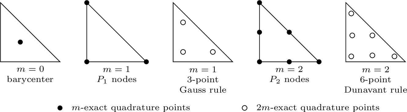

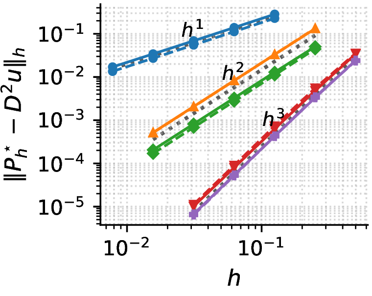
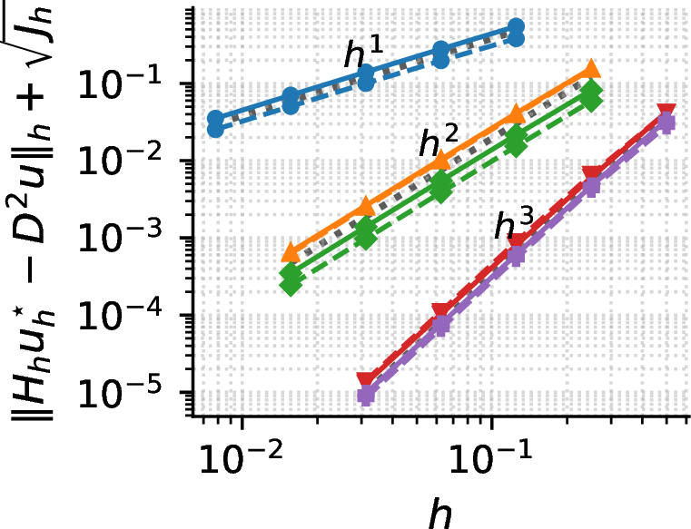
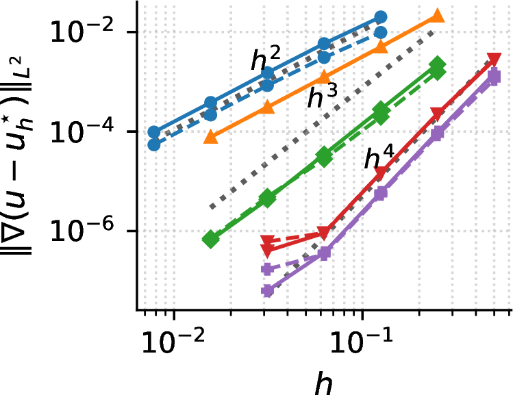
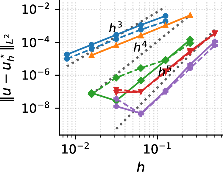
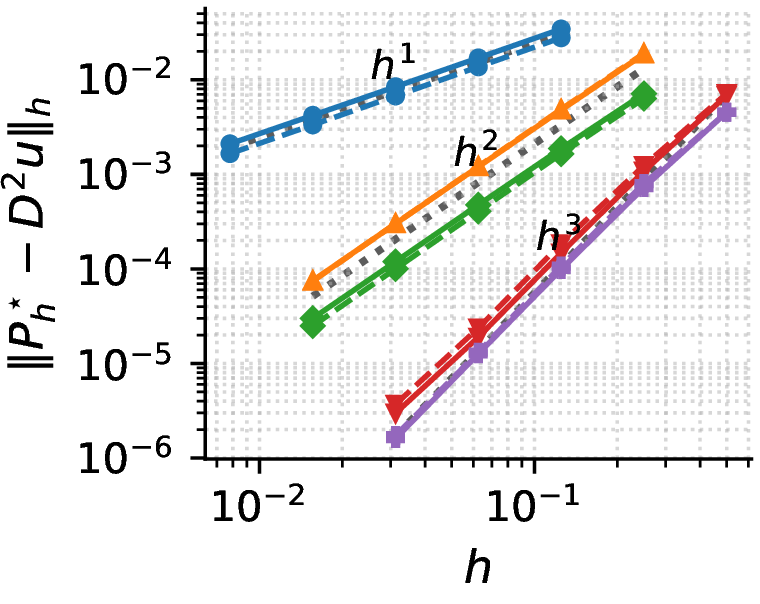
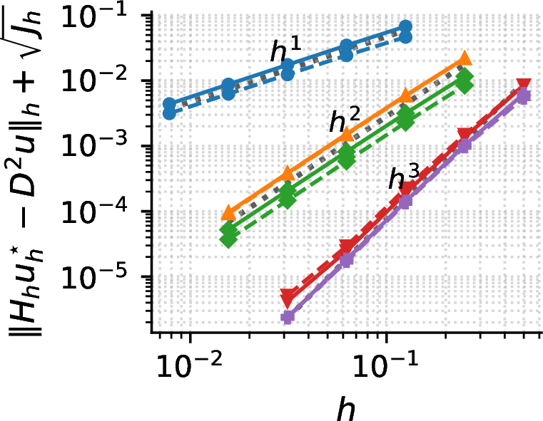

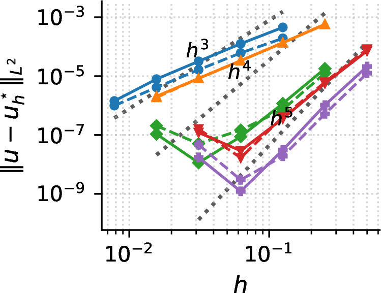
Figure 2: Errors vs. mesh size \(h\) for test cases 1 (top row) and 2 (bottom row). From left to right: the error \(\|\mathbf{P}_h^\star-D^2u\|_h\), the error \(\|H_hu_h^\star-D^2u\|_h + J_h(u_h^\star-u,u_h^\star-u)^{1/2}\), the error \(\|\nabla(u-u_h^\star)\|_{L^2}\) and the error \(\|u-u_h^\star\|_{L^2}\)..

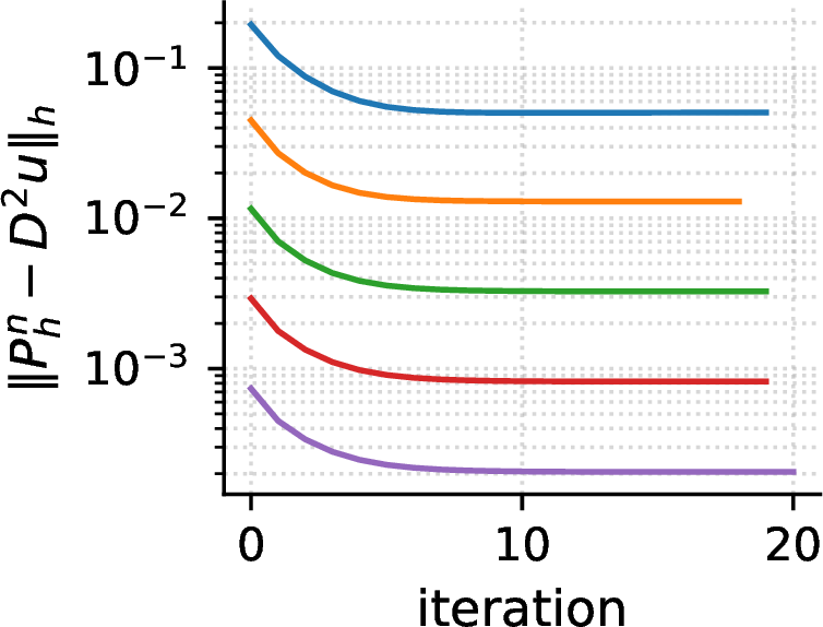
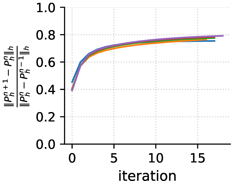
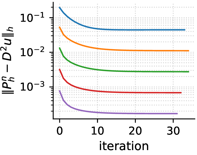
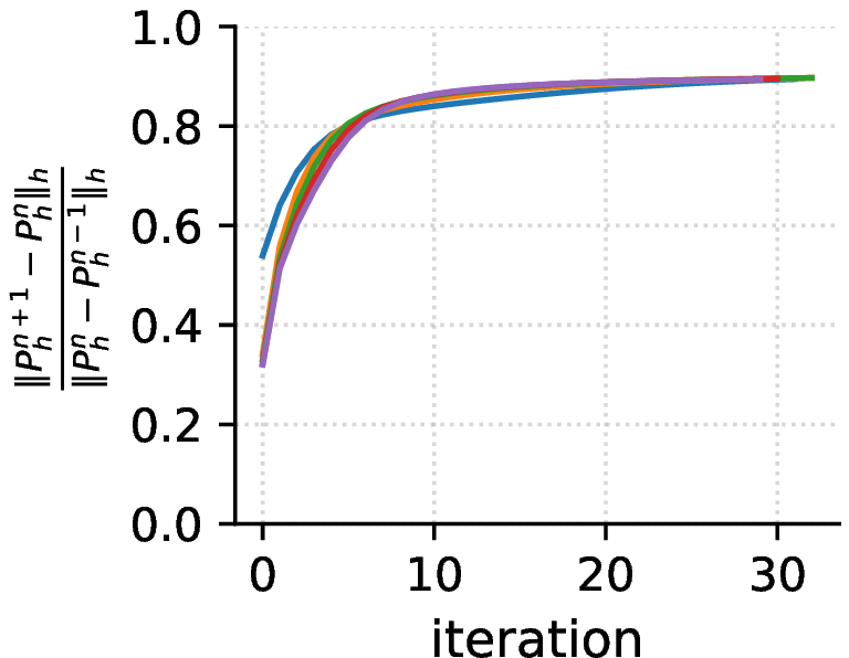

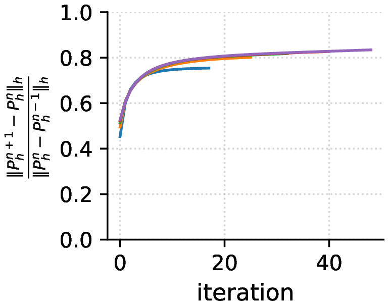
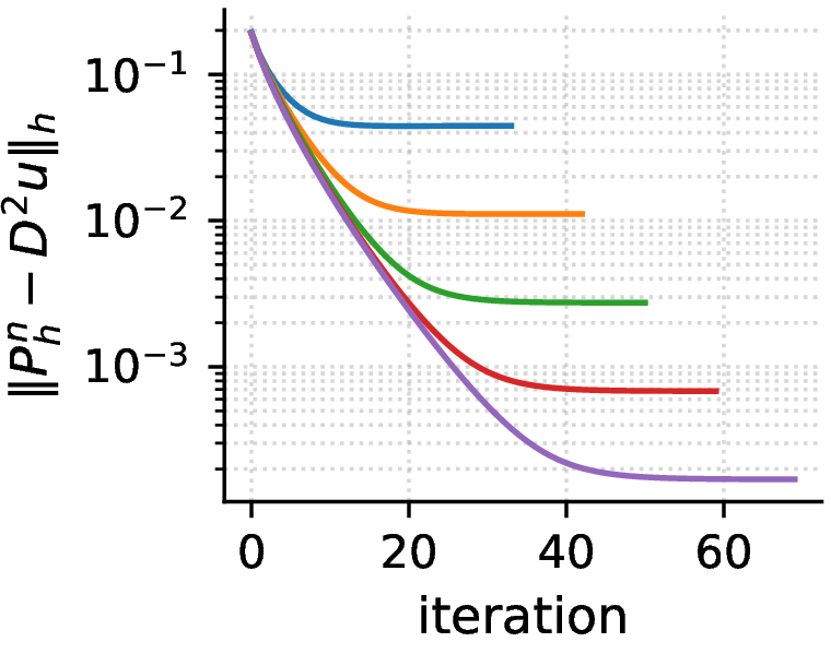
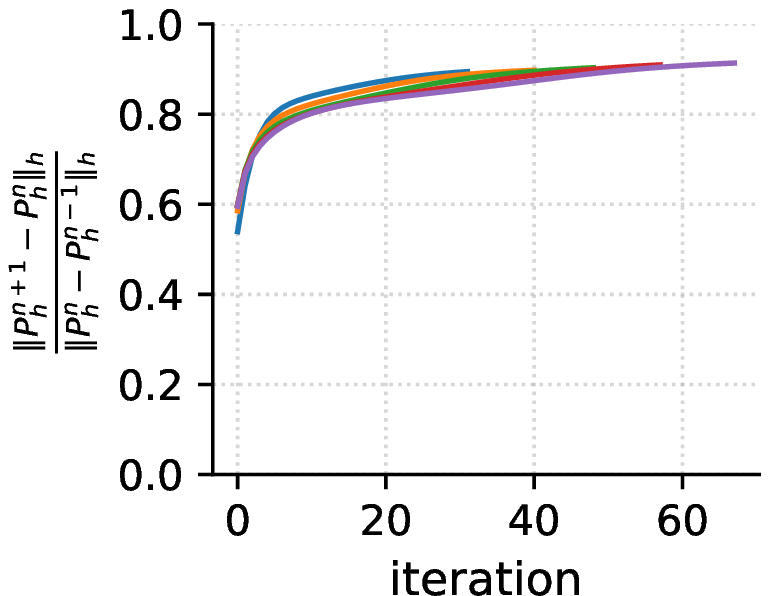
Figure 3: Error and approximated contraction factor vs. iteration \(n\) for two initialization strategies: continuation (top row) and Poisson (bottom row). From left to right: the error \(\|\mathbf{P}_h^n-D^2u\|_h\) and the ratio \(\|\mathbf{P}_h^{n+1}-\mathbf{P}_h^n\|_h/\|\mathbf{P}_h^{n}-\mathbf{P}_h^{n-1}\|_h\) for \(C^0\) finite elements with \(m=1\) and the three-point Gauss rule and for DG finite elements with \(m=1\) and the three-point Gauss rule..
6.2 Test cases↩︎
We consider two manufactured solutions on \(\Omega=[0,1]^2\): \[u_1(x,y)=\exp\!\left(\frac{x^2+y^2}{2}\right), \qquad u_2(x,y)=-\sqrt{4-x^2-y^2}.\] In both cases \(f=\det D^2u_i\) and \(g=u_i|_{\partial\Omega}\). 2 reports the errors as functions of the mesh size \(h\) for both test cases. For both the \(C^0\) and DG methods, the errors \(\|\mathbf{P}_h^\star-D^2u\|_h\) and \(\|H_hu_h^\star-D^2u\|_h + J_h(u_h^\star - u,u_h^\star - u)^{1/2}\) converge with the expected rate \(h^{m+1}\), including the case \(m=0\). For \(m=1,2\), these observations agree with 2 and [cor:conv_c0,cor:convdg]. For \(m=0\), the same rate is observed numerically, although the smallness condition required in [rem:m0c0,rem:m0dg] has not been checked for the present test cases.
The convergence of the \(H^1\) and \(L^2\)-errors, \(\|\nabla(u-u_h^\star)\|_{L^2(\mathcal{T}_h)}\) and \(\|u-u_h^\star\|_{L^2(\mathcal{T}_h)}\) is more sensitive to the choice of the nodal points defining the discrete norm \(\|\cdot\|_h\). For \(m=1\), the natural choice of nodal points, corresponding to a quadrature rule that is exact on \(\mathbb{P}_1\), does not yield the optimal rates for elliptic problems. In contrast, using quadrature points that are exact on \(\mathbb{P}_2\) significantly improves the results. In the \(C^0\) case, this recovers the optimal convergence rates \(h^{m+2}\) and \(h^{m+3}\) for the \(H^1\)- and \(L^2\)-errors, respectively. For the DG method, the optimal \(H^1\)-rate is also observed, whereas the \(L^2\)-error converges more slowly than expected. This behavior may be explained by the poor conditioning of the corresponding linear systems; see Appendix 8.1. For \(m=2\), both choices of nodal points recover the expected \(H^1\)-convergence rate \(h^{m+2}=h^4\), although a slight deterioration is visible on the finest meshes, again consistent with the large condition numbers reported in Appendix 8.1. The optimal \(L^2\)-rate \(h^{m+3}=h^5\) is obtained only when the Dunavant quadrature rule is used, and deteriorates on the finest meshes, where the corresponding linear systems are also increasingly ill-conditioned. Finally, for the lowest-order case \(m=0\), both the \(H^1\) and \(L^2\)-errors converge at a rate close to \(h^2\). While this is the optimal rate for the \(H^1\)-error, it is suboptimal for the \(L^2\)-error, whose expected rate would be \(h^3\).
3 reports the error \(\|\mathbf{P}_h^n-D^2u\|_h\) and the approximated contraction factor \(\|\mathbf{P}_h^{n+1}-\mathbf{P}_h^n\|_h/\|\mathbf{P}_h^{n}-\mathbf{P}_h^{n-1}\|_h\) as functions of the iteration of the splitting algorithm. It also compares the two initialization strategies: the continuation strategy and the initialization based on the Poisson problem 38 . We present only the first test case with \(m=1\) and the three-point Gauss rule, since the second test case and the other parameter choices exhibit similar behavior. For both initialization strategies, the error decreases monotonically with the iteration count. Moreover, after an initial transient, the ratios \(\|\mathbf{P}_h^{n+1}-\mathbf{P}_h^n\|_h/\|\mathbf{P}_h^{n}-\mathbf{P}_h^{n-1}\|_h\) approach comparable values for the different mesh sizes, providing numerical evidence for a mesh-uniform linear convergence rate, consistently with 2. As expected, the continuation strategy requires significantly fewer iterations than the Poisson initialization. Nevertheless, the latter also converges to the same accuracy, albeit more slowly, suggesting that the practical basin of attraction may be larger than the sufficient neighbourhood provided by 2.
7 Conclusions↩︎
We developed a unified framework for the fully discrete convergence analysis of the least-squares splitting method for the Monge-Ampère equation. Under suitable assumptions on the discretization of the linear variational subproblem, namely a discrete Miranda-Talenti inequality and a sufficiently high polynomial degree, we proved local convergence of the iterative method and optimal-order convergence of its fixed point to the exact solution in an \(H^2\)-type norm. We verified these assumptions for representative \(C^1\), \(C^0\), and DG finite element methods using existing discrete Miranda-Talenti estimates. The numerical experiments agree with the theoretical results. In particular, they confirm the predicted convergence rates and indicate that, in the tested cases, the practical basin of attraction is larger than the sufficient \(O(h)\)-neighbourhood established by the analysis.
Although the present analysis does not cover the original low-order discretizations of [18], [20], the framework applies to any reconstruction satisfying the abstract stability and consistency assumptions. It therefore also provides a route to the analysis of other existing or future low-order schemes, once suitable discrete Miranda-Talenti and consistency estimates are established.
Several other directions remain open for future research. These include Monge-Ampère equations with gradient-dependent right-hand sides and second boundary conditions, in particular those arising in optimal transport and related problems. Another natural direction is the extension of the framework to other uniformly elliptic fully nonlinear operators.
Acknowledgments↩︎
The author is grateful to Mohamed Ben Abdelouahab, Alexandre Caboussat and Marco Picasso for fruitful discussions.
8 Additional numerical results↩︎
We report some additional numerical results to complement those in the main body of the manuscript.
8.1 Condition numbers↩︎
The matrices arising from the assembly of \(a_h\) become increasingly ill-conditioned under mesh refinement, with observed condition numbers growing approximately as \(h^{-4}\), see ¿tbl:tab:condition95numbers?. The condition number is slightly better for \(\mathbb{P}_{2m}\) exact quadrature nodes.
8.2 Comparison of different values of \(\sigma\)↩︎
We investigate the influence of the parameter \(\sigma\in\{1,2,5,20\}\) for the first test case. 4 reports the \(H^2\)-type error as a function of the mesh size \(h\), while 5 shows the convergence history together with the ratio \(\|\mathbf{P}_h^{n+1}-\mathbf{P}_h^n\|_h/\|\mathbf{P}_h^{n}-\mathbf{P}_h^{n-1}\|_h\). The results indicate that, although \(\sigma\) affects the convergence rate, consistently with 2, the iteration converges for all values considered, and the convergence with respect to \(h\) is essentially unchanged.
| \(C^0\) | DG | ||||||
|---|---|---|---|---|---|---|---|
| \(m\) | points | \(h_1\) | \(h_2\) | \(h_3\) | \(h_1\) | \(h_2\) | \(h_3\) |
| \(0\) | barycenter | \(10^{7}\) | \(2\times 10^{8}\) | \(3\times 10^{9}\) | \(3\times 10^{7}\) | \(4\times 10^{8}\) | \(7\times 10^{9}\) |
| \(1\) | \(\mathbb{P}_1\) nodes | \(2\times 10^{7}\) | \(3\times 10^{8}\) | \(4\times 10^{9}\) | \(6\times 10^{7}\) | \(9\times 10^{8}\) | \(10^{10}\) |
| \(1\) | Gauss | \(6\times 10^{6}\) | \(10^{8}\) | \(2\times 10^{9}\) | \(2\times 10^{7}\) | \(4\times 10^{8}\) | \(6\times 10^{9}\) |
| \(2\) | \(\mathbb{P}_2\) nodes | \(10^{7}\) | \(2\times 10^{8}\) | \(3\times 10^{9}\) | \(3\times 10^{7}\) | \(5\times 10^{8}\) | \(7\times 10^{9}\) |
| \(2\) | Dunavant | \(2\times 10^{6}\) | \(4\times 10^{7}\) | \(6\times 10^{8}\) | \(9\times 10^{6}\) | \(10^{8}\) | \(2\times 10^{9}\) |
| \(C^0\) | DG | ||||||
|---|---|---|---|---|---|---|---|
| \(m\) | points | \(h_1\) | \(h_2\) | \(h_3\) | \(h_1\) | \(h_2\) | \(h_3\) |
| \(0\) | barycenter | \(10^{7}\) | \(2\times 10^{8}\) | \(2\times 10^{9}\) | \(2\times 10^{7}\) | \(4\times 10^{8}\) | \(6\times 10^{9}\) |
| \(1\) | \(\mathbb{P}_1\) nodes | \(10^{7}\) | \(2\times 10^{8}\) | \(3\times 10^{9}\) | \(4\times 10^{7}\) | \(6\times 10^{8}\) | \(10^{10}\) |
| \(1\) | Gauss | \(6\times 10^{6}\) | \(9\times 10^{7}\) | \(10^{9}\) | \(2\times 10^{7}\) | \(3\times 10^{8}\) | \(4\times 10^{9}\) |
| \(2\) | \(\mathbb{P}_2\) nodes | \(9\times 10^{6}\) | \(10^{8}\) | \(2\times 10^{9}\) | \(2\times 10^{7}\) | \(3\times 10^{8}\) | \(5\times 10^{9}\) |
| \(2\) | Dunavant | \(2\times 10^{6}\) | \(3\times 10^{7}\) | \(5\times 10^{8}\) | \(6\times 10^{6}\) | \(9\times 10^{7}\) | \(10^{9}\) |
| \(C^0\) | DG | ||||||
|---|---|---|---|---|---|---|---|
| \(m\) | points | \(h_1\) | \(h_2\) | \(h_3\) | \(h_1\) | \(h_2\) | \(h_3\) |
| \(0\) | barycenter | \(10^{7}\) | \(2\times 10^{8}\) | \(3\times 10^{9}\) | \(3\times 10^{7}\) | \(4\times 10^{8}\) | \(7\times 10^{9}\) |
| \(1\) | \(\mathbb{P}_1\) nodes | \(10^{7}\) | \(2\times 10^{8}\) | \(3\times 10^{9}\) | \(3\times 10^{7}\) | \(4\times 10^{8}\) | \(7\times 10^{9}\) |
| \(1\) | Gauss | \(6\times 10^{6}\) | \(10^{8}\) | \(2\times 10^{9}\) | \(2\times 10^{7}\) | \(2\times 10^{8}\) | \(4\times 10^{9}\) |
| \(2\) | \(\mathbb{P}_2\) nodes | \(8\times 10^{6}\) | \(10^{8}\) | \(2\times 10^{9}\) | \(2\times 10^{7}\) | \(2\times 10^{8}\) | \(4\times 10^{9}\) |
| \(2\) | Dunavant | \(2\times 10^{6}\) | \(3\times 10^{7}\) | \(5\times 10^{8}\) | \(5\times 10^{6}\) | \(7\times 10^{7}\) | \(10^{9}\) |
| \(C^0\) | DG | ||||||
|---|---|---|---|---|---|---|---|
| \(m\) | points | \(h_1\) | \(h_2\) | \(h_3\) | \(h_1\) | \(h_2\) | \(h_3\) |
| \(0\) | barycenter | \(2\times 10^{7}\) | \(3\times 10^{8}\) | \(5\times 10^{9}\) | \(4\times 10^{7}\) | \(6\times 10^{8}\) | \(10^{10}\) |
| \(1\) | \(\mathbb{P}_1\) nodes | \(10^{7}\) | \(2\times 10^{8}\) | \(3\times 10^{9}\) | \(3\times 10^{7}\) | \(4\times 10^{8}\) | \(7\times 10^{9}\) |
| \(1\) | Gauss | \(8\times 10^{6}\) | \(10^{8}\) | \(2\times 10^{9}\) | \(2\times 10^{7}\) | \(3\times 10^{8}\) | \(5\times 10^{9}\) |
| \(2\) | \(\mathbb{P}_2\) nodes | \(8\times 10^{6}\) | \(10^{8}\) | \(2\times 10^{9}\) | \(10^{7}\) | \(2\times 10^{8}\) | \(3\times 10^{9}\) |
| \(2\) | Dunavant | \(2\times 10^{6}\) | \(4\times 10^{7}\) | \(6\times 10^{8}\) | \(5\times 10^{6}\) | \(8\times 10^{7}\) | \(10^{9}\) |
| \(C^0\) | DG | ||||||
|---|---|---|---|---|---|---|---|
| \(m\) | points | \(h_1\) | \(h_2\) | \(h_3\) | \(h_1\) | \(h_2\) | \(h_3\) |
| \(0\) | barycenter | \(3\times 10^{7}\) | \(5\times 10^{8}\) | \(8\times 10^{9}\) | \(6\times 10^{7}\) | \(9\times 10^{8}\) | \(2\times 10^{10}\) |
| \(1\) | \(\mathbb{P}_1\) nodes | \(2\times 10^{7}\) | \(3\times 10^{8}\) | \(5\times 10^{9}\) | \(3\times 10^{7}\) | \(5\times 10^{8}\) | \(8\times 10^{9}\) |
| \(1\) | Gauss | \(10^{7}\) | \(2\times 10^{8}\) | \(3\times 10^{9}\) | \(3\times 10^{7}\) | \(4\times 10^{8}\) | \(6\times 10^{9}\) |
| \(2\) | \(\mathbb{P}_2\) nodes | \(9\times 10^{6}\) | \(10^{8}\) | \(2\times 10^{9}\) | \(2\times 10^{7}\) | \(2\times 10^{8}\) | \(4\times 10^{9}\) |
| \(2\) | Dunavant | \(3\times 10^{6}\) | \(5\times 10^{7}\) | \(9\times 10^{8}\) | \(6\times 10^{6}\) | \(10^{8}\) | \(2\times 10^{9}\) |
\(\sigma=1\)
\(\sigma=2\)
\(\sigma=5\)
\(\sigma=10\)
\(\sigma=20\)
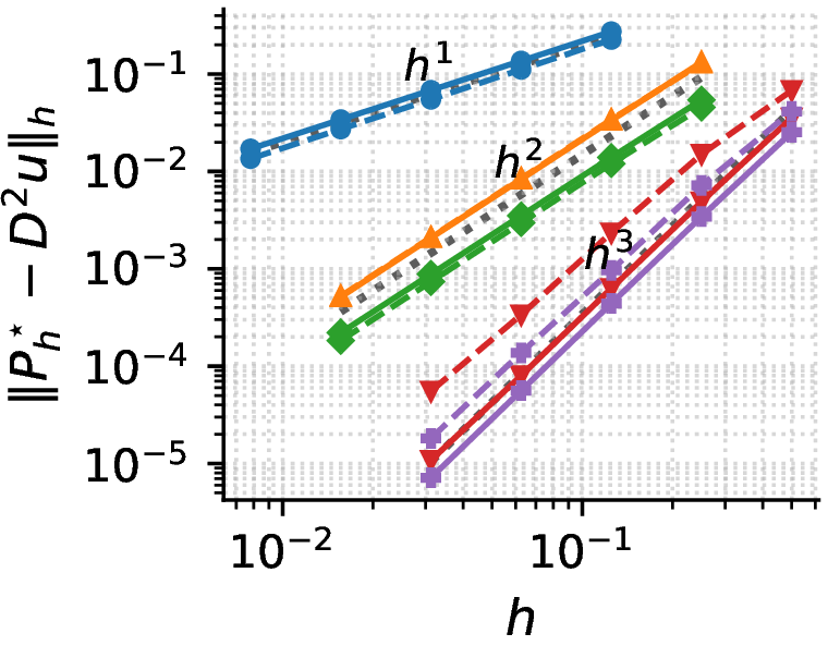
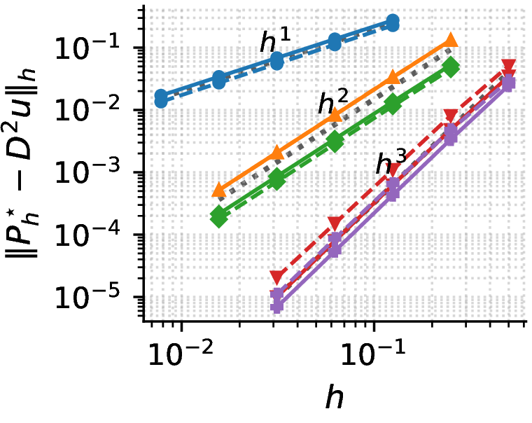
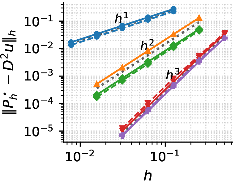
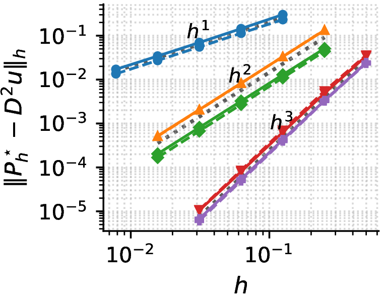
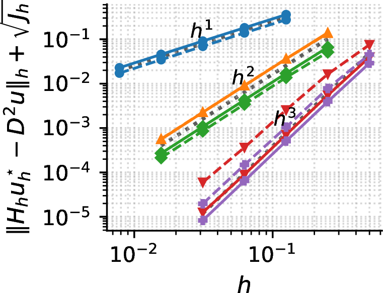
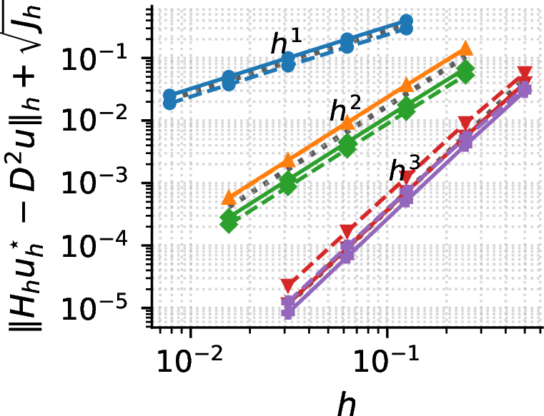
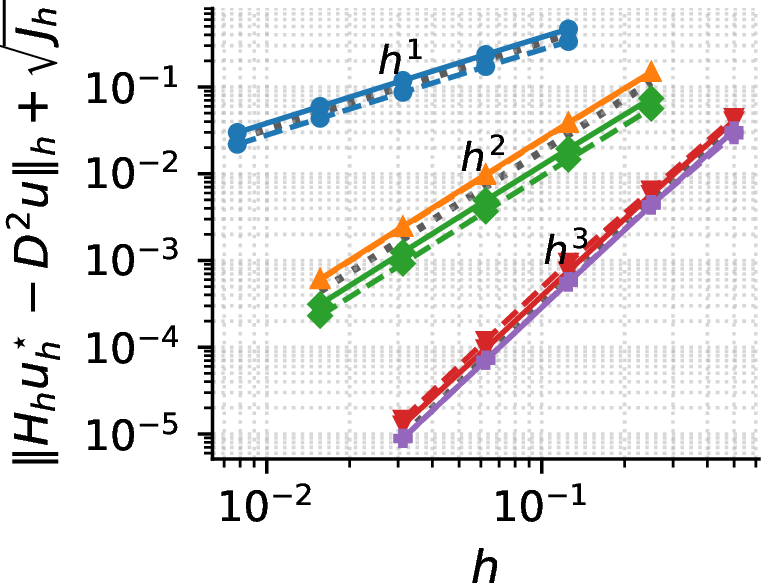
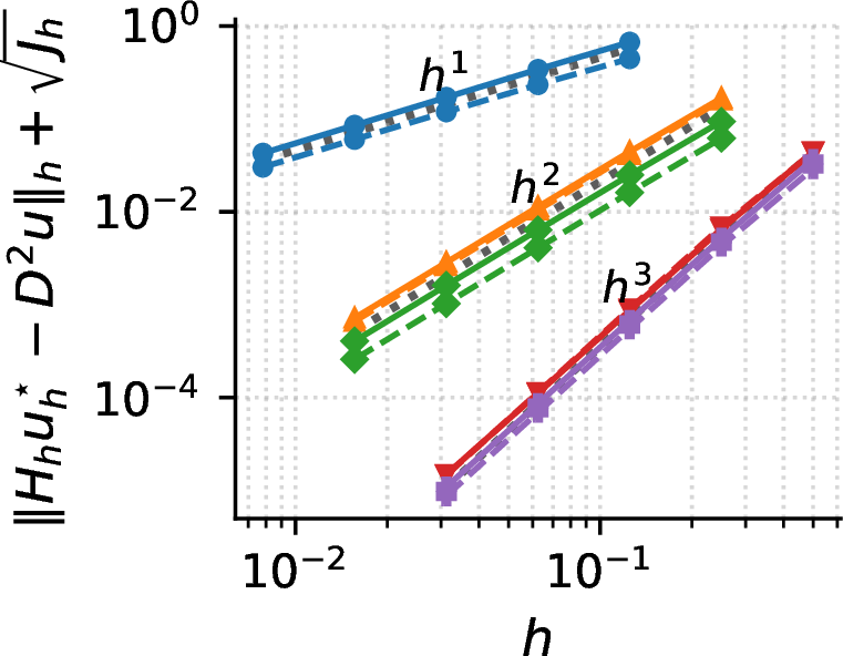
Figure 4: Columns (from left to right) correspond to \(\sigma=1\), \(2\), \(5\), and \(20\). The top row shows \(\|\mathbf{P}_h^\star-D^2u\|_h\), while the bottom row shows \(\|H_hu_h^\star-D^2u\|_h + J_h(u_h^\star-u,u_h^\star-u)^{1/2}\), both as functions of the mesh size \(h\) for test case 1..
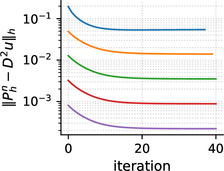
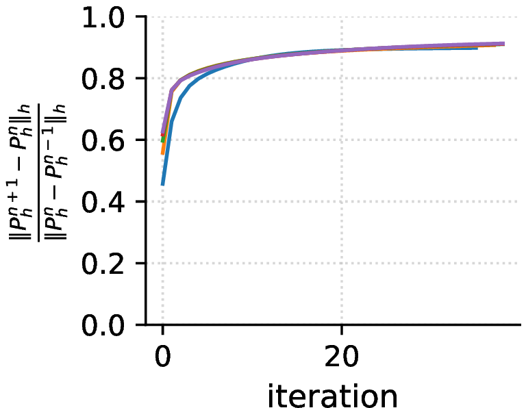
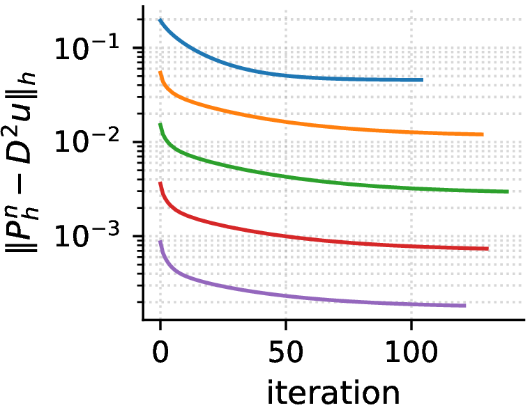
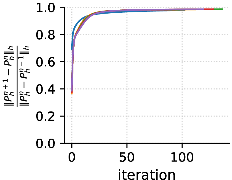
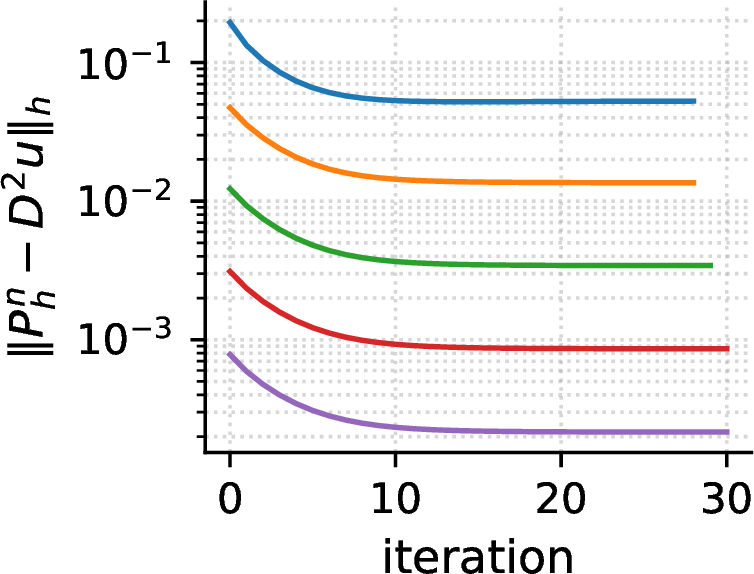
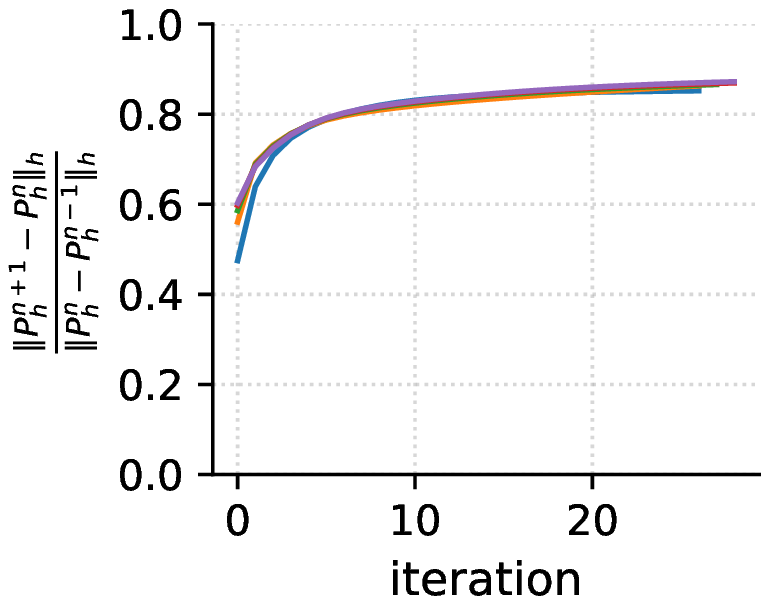
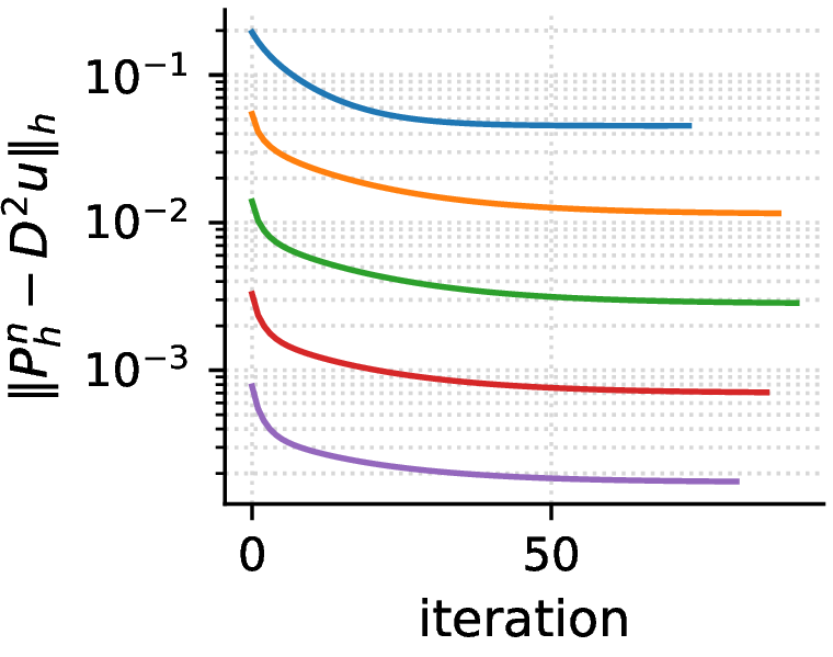
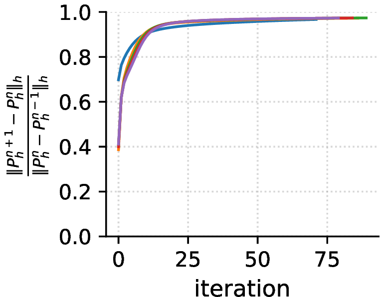
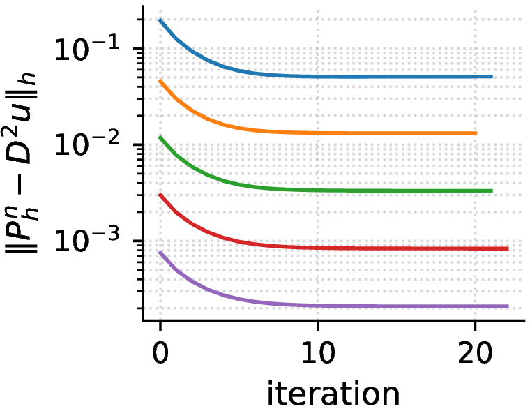
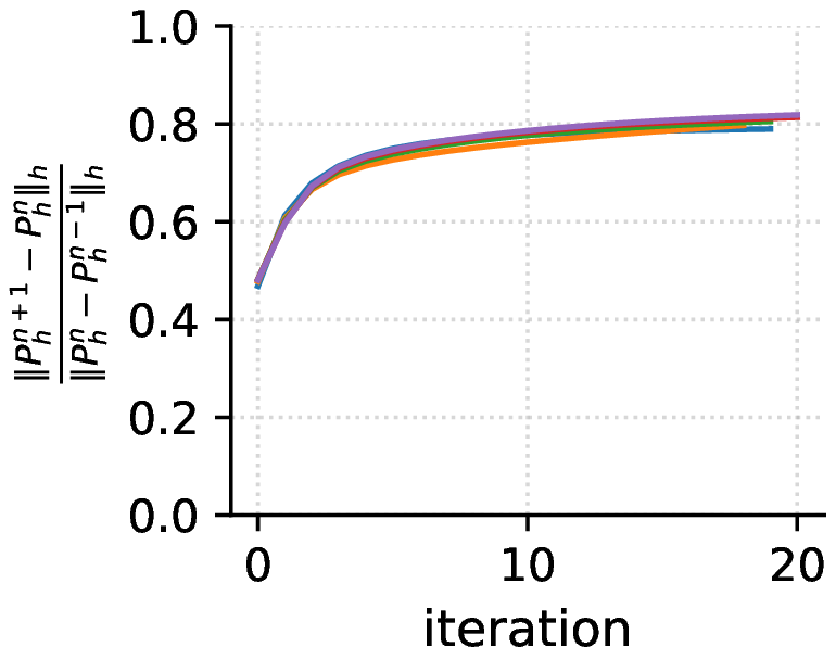
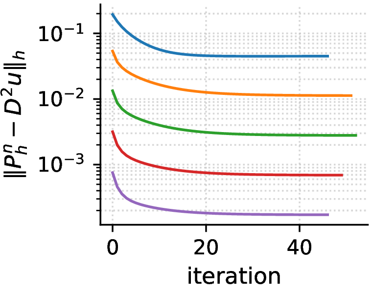
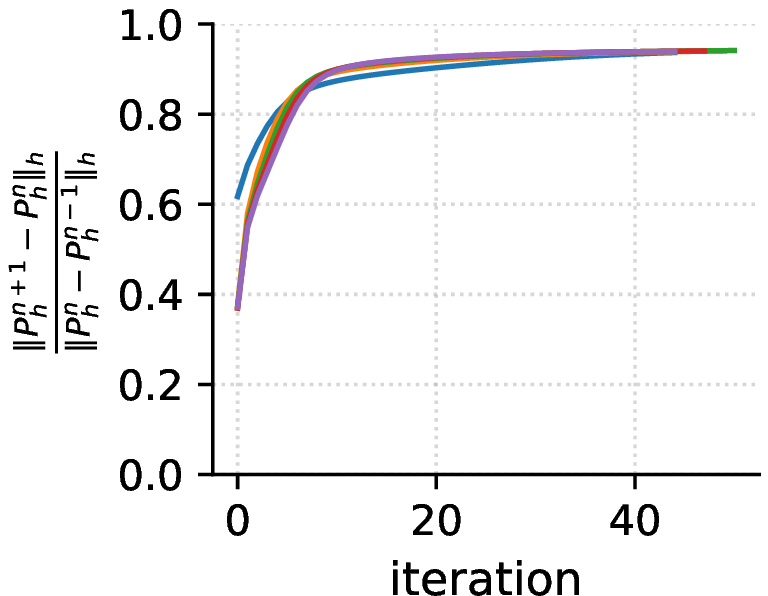
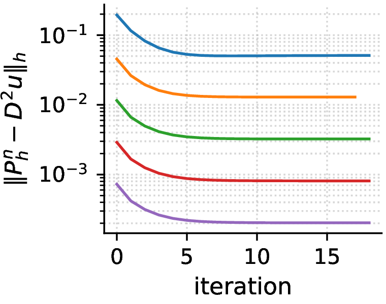
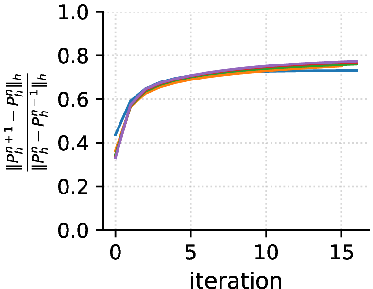
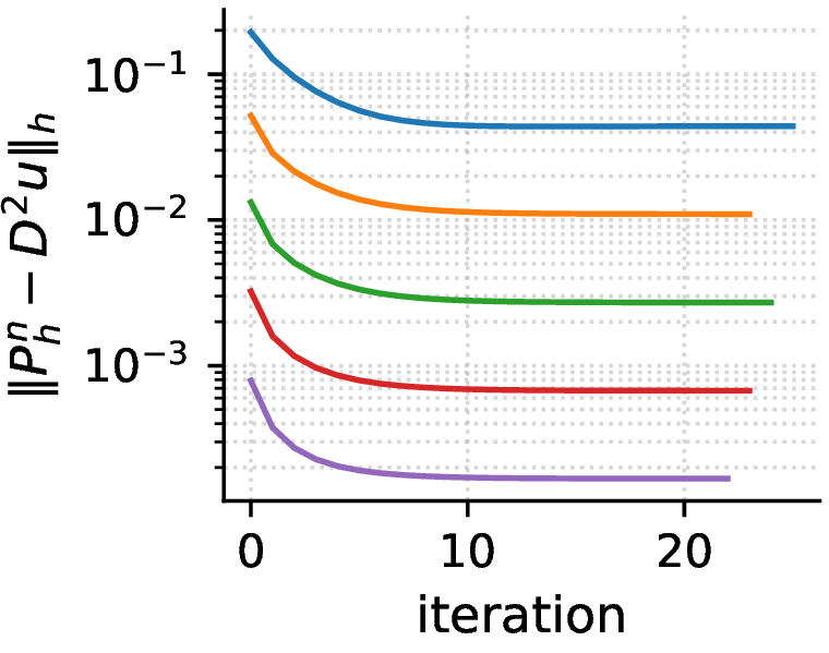

Figure 5: Error and approximated contraction factor vs. iteration \(n\) for \(\sigma=1\) (first row), \(2\) (second row), \(5\) (third row), and \(20\) (fourth row). From left to right: the error \(\|\mathbf{P}_h^n-D^2u\|_h\) and the ratio \(\|\mathbf{P}_h^{n+1}-\mathbf{P}_h^n\|_h/\|\mathbf{P}_h^{n}-\mathbf{P}_h^{n-1}\|_h\) for \(C^0\) finite elements with \(m=1\) and the three-point Gauss rule and for DG finite elements with \(m=1\) and the three-point Gauss rule..