JADE-GS: Joint Alternating Deblurring Guided by Events in 3D Gaussian Splatting
July 16, 2026
Abstract
When a camera moves fast during exposure, blur destroys the intra-exposure motion a 3D model needs to recover the sharp scene, while event cameras capture exactly this signal at microsecond resolution. Turning them into reliable 3D supervision faces two obstacles. First, the two restoration priors fail in opposite ways: physics-based event-integration priors preserve edges but accumulate drift; learned networks recover texture but distort boundaries. Second, existing pipelines run in one direction only, so raw event noise or the biases of fixed 2D pseudo-labels pass uncorrected into the geometry. JADE-GS addresses both: a pixel-adaptive routing gate fuses the complementary priors, and the resulting 2D restorer is coupled to a 3D Gaussian Splatting student in a bidirectional loop, where detached, multi-view-consistent renders and a physics-based reblurring constraint regularize the restorer, turning a fixed preprocessor into a geometry-aware predictor. Across synthetic and real benchmarks, JADE-GS attains the best perceptual quality, leading LPIPS and CLIP-IQA on both benchmarks with competitive PSNR and SSIM, and trains in about one hour under 5 GB on a single consumer GPU while preserving real-time rendering. Code is available at https://github.com/rootlesswater/JADE-GS.
1 Introduction↩︎
High-quality 3D reconstruction and novel-view synthesis rest on a simple premise: the training images faithfully depict the scene from each viewpoint. Both implicit radiance fields [1] and explicit 3D Gaussian Splatting [2] rely on it to fit consistent geometry across views. Motion blur breaks it: under fast camera motion or long exposure, each frame integrates a range of poses within the exposure window, the reconstruction inherits the degradation as blurred appearance and inconsistent geometry [3]–[5]. Undoing this requires the intra-exposure motion trajectory, which a blurry frame alone cannot provide: its limited temporal resolution has already averaged that motion away.
Event cameras [6], [7] supply precisely this signal. Reporting brightness changes asynchronously at microsecond resolution, they preserve the intra-exposure motion that the exposure integral erases, and stay informative in the low-light, high-speed regimes where lengthening the RGB exposure only adds blur [8], [9]. This complementarity has driven a growing literature coupling events with frames, first for 2D deblurring [10]–[12] and recently for 3D reconstruction [13]–[17]. Following these benchmarks, we target ego-motion blur of a static scene under a fast-moving camera, which is also the setting considered by prior event-guided 3D deblurring methods.
1.0.0.1 State of the art and its limitations.
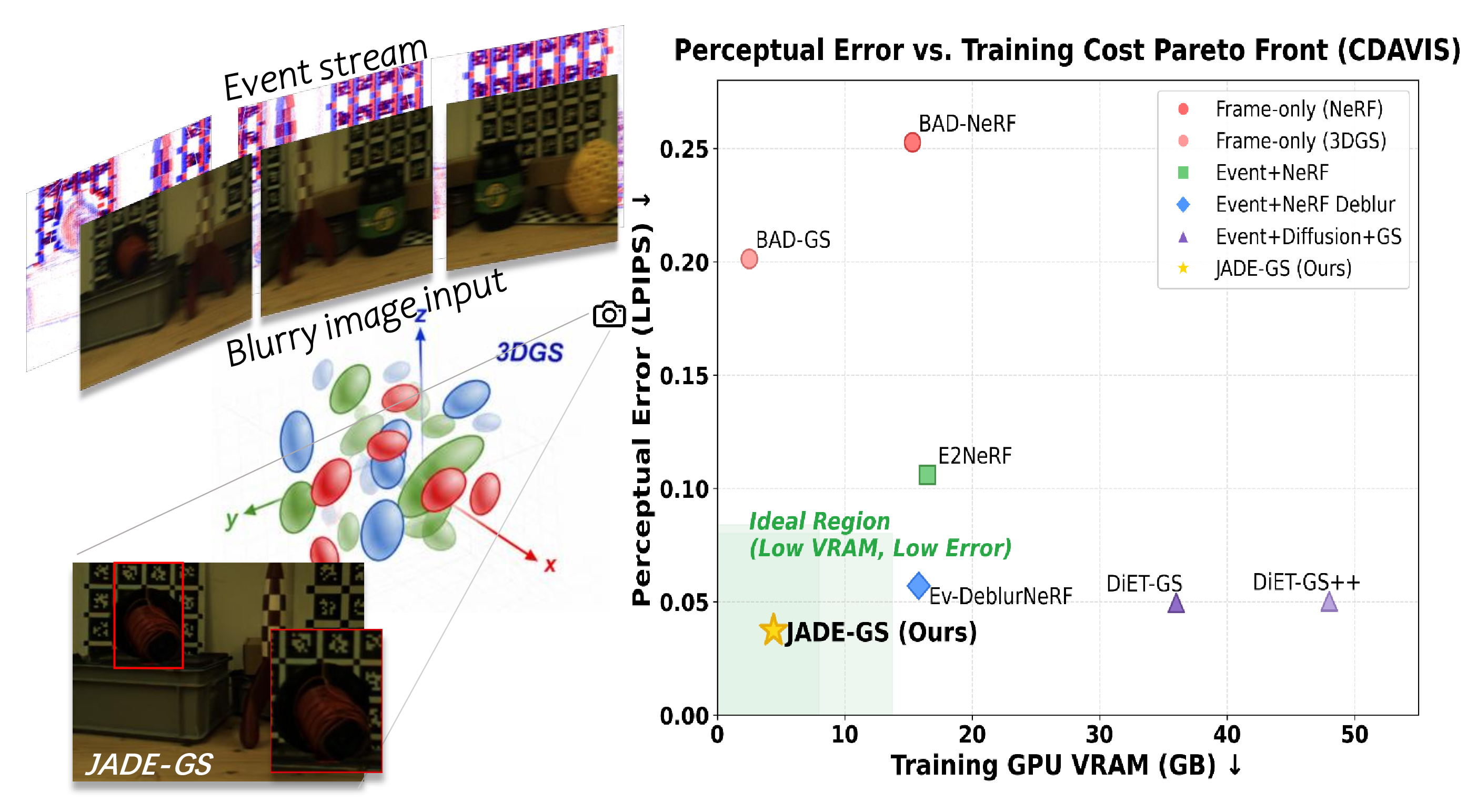
Existing event-guided deblurring 3D methods fall into two categories. The first treats restoration as a fixed preprocess: it pre-deblurs every training frame with a frozen 2D model—either a physical event-integration prior [10] or a learned network [11]—and then feeds the output to a standard 3DGS pipeline that never revisits the deblurring stage. This one-directional cascade is simple but brittle: the 3D module has no way to correct artifacts in the 2D pseudo-labels, so EDI’s drift and noise appear in the final model. The second category [15], [16] couples a coarse-to-fine NeRF with an event-guided deblurring module, but the per-pixel MLP sampling of NeRF makes end-to-end training expensive (10+ hours, 15+ GB), limiting adoption.
JADE-GS resolves the dilemma with three components. (i) A pixel-adaptive routing gate blends EDI and EFNet outputs at each pixel, inheriting EDI’s edge fidelity where events are reliable and EFNet’s texture quality where they are not. (ii) A bidirectional teacher-student loop turns the 3DGS renderer from a passive consumer of pseudo-labels into a multi-view regularizer. On the forward pass the teacher deblurs each training view; on the backward pass the student’s disconnected renders are re-blurred via the physical event model and compared to the observed blur, back-propagating 3D-consistent corrections into the teacher’s gate. (iii) The student is a 3DGS model that inherits real-time rendering and low-memory training. Together, the method trains in \(\sim\)1 hour under 5 GB on a single consumer GPU while preserving real-time rendering and producing the best perceptual results among all baselines.
1.0.0.2 Contributions.
We identify that EDI (physics) and EFNet (learning) restore complementary but individually incomplete pseudo-labels, and propose a pixel-adaptive routing gate that fuses them based on per-pixel reliability.
We introduce a bidirectional teacher-student framework where 3DGS renders regularize the 2D restorer through a physical reblurring constraint, closing the loop between deblurring and geometry.
We establish a new state-of-the-art on the EvDeblur-CDAVIS real benchmark, leading LPIPS (0.0374) and CLIP-IQA (0.2564) with competitive PSNR (34.17) and runner-up SSIM (0.9207), and identical findings on the synthetic Blur-NeRF-Synth benchmark.
Training is practical: \(\sim\)1 hour and under 5 GB GPU memory on a single RTX 5090, roughly a 10\(\times\) speedup and 4\(\times\) memory reduction versus event-based NeRF methods.
2 Related Work↩︎
2.0.0.1 3DGS and blur-aware reconstruction.
Neural Radiance Fields [1], [18] achieve high-quality view synthesis but at heavy computational cost, which 3D Gaussian Splatting [2] alleviates by replacing the implicit field with explicit point-based rasterization for fast optimization and real-time rendering. To make either representation robust to blur, a family of methods explicitly models the image formation process, either as an exposure integral over the trajectory or as a per-view blur kernel [3]–[5], [19], [20]. They differ in where the kernel lives and how it is parameterized, but share one assumption: that the blur can be inverted from RGB alone. This breaks down under severe motion, where a single frame retains too little of the trajectory to constrain the solution; recovering that lost motion is what an auxiliary sensor provides.
2.0.0.2 Event-based 2D deblurring.
Event cameras supply that missing motion signal, and 2D deblurring is where methods for exploiting it first matured. The two ends of the spectrum are analytical and learned: the Event Double Integral (EDI) [10] inverts the blur directly from event physics, while fusion networks such as EFNet [11] learn the mapping from paired frames and events. Most recent work concerns how best to combine the two modalities rather than which to choose, through asymmetric hierarchical fusion [8], spatial-temporal collaboration [12], or motion-adaptive attention driven by event masks [9]. This consistent complementarity motivates our fusion; the difference is that we carry it into a 3D-consistent loop rather than stopping at a single 2D output.
2.0.0.3 Event-based 3D reconstruction and deblurring.
A parallel line lifts events into 3D, first through NeRF [13], [14] and then into 3DGS [17], [21]–[23]. For deblurring, existing systems couple restoration and reconstruction in one direction only, in one of two ways. The first family injects the event-generation model directly into the 3D objective: E\(^2\)NeRF [15] and Ev-DeblurNeRF [16] supervise the field with event and blur-formation losses, and recent 3DGS systems follow suit while extending orthogonal axes such as intra-exposure pose optimization [24], SfM-free initialization [25], event-only large-scale capture [26], and asynchronous high-resolution rigs [27]; the 3D model must then disentangle geometry from raw event physics alone, with no learned restoration prior to absorb threshold mismatch and integration noise. The second family interposes a 2D restorer or generative prior whose pseudo-sharp targets are consumed as fixed labels [28]; any 2D bias is frozen into the geometry [29], and multi-view consistency cannot restore detail that the labels never contained [17], [24], [25]. JADE-GS sits between the two: it keeps a learned restorer in the loop, but lets the 3D student regularize it in return.
2.0.0.4 Teacher–student coupling.
Transferring knowledge from an expressive teacher to a compact student is a long-standing tool in image restoration [30], but in the standard setup the teacher is fixed and only the student learns. Our coupling is bidirectional: the 2D restorer supplies pseudo-sharp supervision to the 3D student, and the student, through detached and multi-view-consistent renders, regularizes the restorer in turn. This mutual refinement, rather than one-way distillation, is what separates JADE-GS from event-guided preprocessing pipelines.
3 Method↩︎
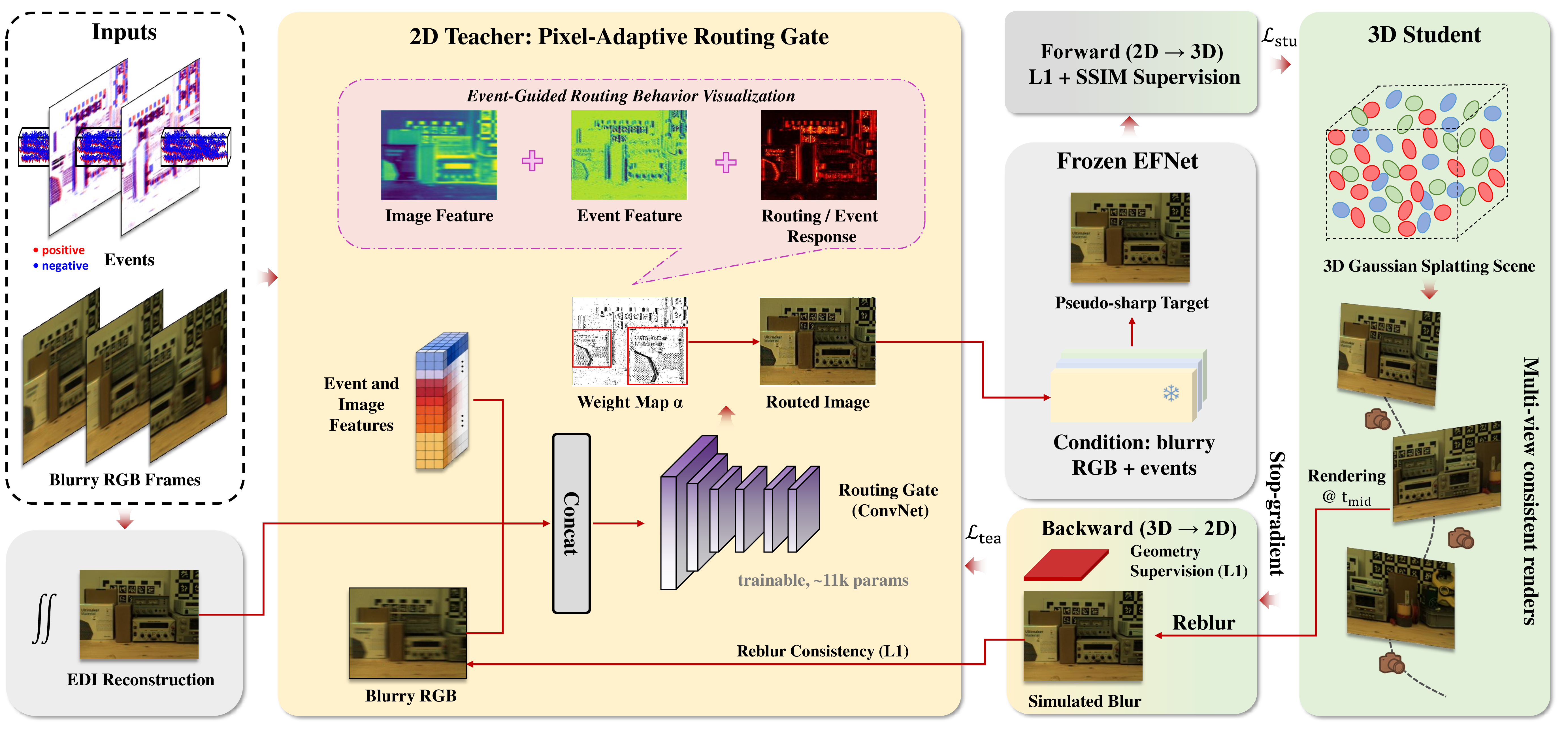
JADE-GS couples a lightweight 2D teacher with a 3D Gaussian Splatting student in a single bidirectional loop (Fig. 2). The teacher fuses a physics-based and a learned restoration prior into a pseudo-sharp target that supervises the student; the student, in turn, feeds its multi-view-consistent renders back to regularize the teacher. We first fix notation (Sec. 3.1), describe how the two priors are fused by a pixel-adaptive gate (Secs. 3.2–3.3), and then close the loop between teacher and student (Sec. 3.4).
3.1 Setup and Notation↩︎
Let \(I^{\star}(t)\) denote the latent sharp image at a continuous camera pose \(\pi(t)\), and let \(B\) be the observed blurry frame produced by finite-exposure integration over \([t_s,t_e]\): \[B = \frac{1}{t_e-t_s}\int_{t_s}^{t_e} I^{\star}(t)\,dt + \epsilon_b, \label{eq:blur}\tag{1}\] where \(\epsilon_b\) absorbs sensor noise, exposure mismatch and residual misalignment. We target the sharp rendering at mid-exposure \(t_{\mathrm{mid}}=(t_s+t_e)/2\). The synchronized event stream is \(E=\{(x_i,y_i,t_i,p_i)\}_{i=1}^{N}\), where each event \((x_i,y_i,t_i,p_i)\) fires when the log-intensity change at pixel \((x_i,y_i)\) exceeds a contrast threshold \(\Theta\), with polarity \(p_i\in\{+1,-1\}\).
We denote the 2D teacher by \(\mathcal{R}\) and the 3D student by \(\mathcal{G}\). The teacher predicts a pseudo-sharp frame \(I_{\mathrm{pseudo}}\) from \(B\) and \(E\), while the student renders a view-consistent estimate \(\hat{I}_{\mathrm{render}}=\mathcal{G}(\pi)\) from the current scene parameters; JADE-GS makes each supervise the other within one loop (Fig. 2).
3.2 Complementary Feature Priors↩︎
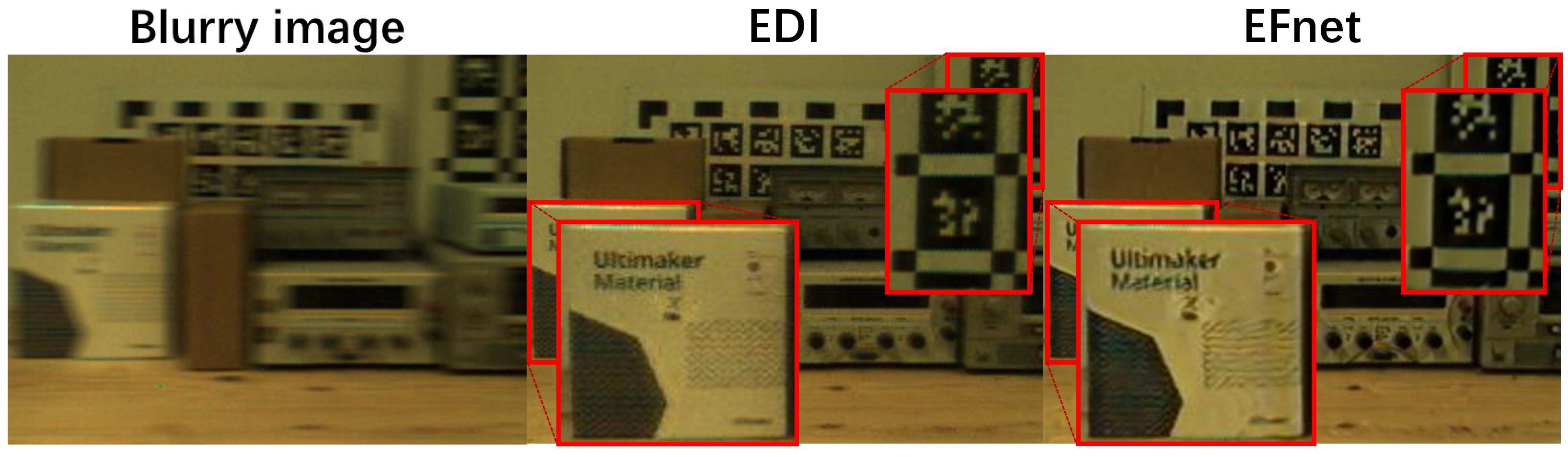
The analytical EDI prior preserves structural edges but exhibits integration drift and weak texture, whereas EFNet yields cleaner texture but can over-smooth or distort boundaries under domain shift (illustrated in the supplement). We select them not as a claimed optimal pair, but as representative, code-available priors from the analytical and learned paradigms whose complementarity is repeatedly documented [8], [12]: EDI’s boundary localization follows directly from event physics and is stable under domain shift, at the cost of accumulated integration noise, while EFNet learns strong texture recovery but can degrade edges when event statistics leave its training domain. The teacher therefore routes toward EDI where physically grounded edge cues are strong, and defers to EFNet where richer texture completion helps.
We first compute an analytical EDI reconstruction \(I_{\mathrm{edi}}=\Phi_{\mathrm{edi}}(B,E)\) and pair it with the blurry frame \(B\) and a temporally binned event-voxel grid \(V(E)\). These signals form the teacher input \[X_{\mathrm{in}} = \big[\,B,\; V(E),\; \tilde{I}_{\mathrm{edi}}\,\big], \label{eq:input}\tag{2}\] where \(\tilde{I}_{\mathrm{edi}}\) is the EDI reconstruction spatially aligned to the event-voxel grid. From \(X_{\mathrm{in}}\) the teacher predicts the pixel-adaptive routing map of Sec. 3.3.
3.3 Pixel-Adaptive Routing↩︎
Rather than a fixed hand-designed blend, we adopt a lightweight pixel-adaptive gate. The routing head is a three-layer convolutional module applied to an 18-channel concatenation: the blurry RGB frame (\(3\)), the EDI reconstruction (\(3\)), shallow event features (\(4\)) and shallow image features (\(8\)). It outputs a per-pixel scalar \(\alpha\in[0,1]\), and the routed result is \[I_{\mathrm{routed}} = \alpha\cdot\tilde{I}_{\mathrm{edi}} + (1-\alpha)\cdot B, \label{eq:route}\tag{3}\] so \(\alpha\!\to\!1\) selects the EDI edge prior and \(\alpha\!\to\!0\) falls back to the blurry observation. The gate is fully learnable and, without any explicit edge label, tends to up-weight EDI in edge-rich regions and revert to the blurry observation in drift-prone flat areas (Sec. 4.6). The routed image, together with the event voxels, is then passed through the frozen EFNet branch to form the pseudo-sharp target \(I_{\mathrm{pseudo}}=\mathrm{EFNet}(I_{\mathrm{routed}},V(E))\). EFNet was trained on blurry inputs while the routed image is partially sharpened, but the deviation is confined to \(\alpha\!\to\!1\) regions, and the backward supervision of Sec. 3.4 adapts the gate toward routed inputs whose refinements the student can reproduce across views; the frozen refiner remains effective in practice (Table 2).
3.4 Bidirectional 2D–3D Coupling↩︎
3.4.0.1 Forward (2D\(\rightarrow\)3D).
The student renders the current view \(\hat{I}_{\mathrm{render}}=\mathcal{G}(\pi)\) and is supervised by the teacher’s pseudo-sharp target through a photometric and structural term: \[\mathcal{L}_{\mathrm{stu}} = \big\|\hat{I}_{\mathrm{render}}-I_{\mathrm{pseudo}}\big\|_1 +\lambda_{\mathrm{ssim}}\,\mathcal{L}_{\mathrm{SSIM}} \big(\hat{I}_{\mathrm{render}},I_{\mathrm{pseudo}}\big). \label{eq:lstu}\tag{4}\]
3.4.0.2 Backward (3D\(\rightarrow\)2D).
If the loop stopped here, any bias in \(I_{\mathrm{pseudo}}\) would be frozen into the geometry, so we let the student regularize the teacher in return. Crucially, the backward signal acts on the routed output \(I_{\mathrm{routed}}=\mathcal{R}(X_{\mathrm{in}})\) rather than on \(I_{\mathrm{pseudo}}\): since EFNet is frozen, all backward gradients update only the routing gate, and no gradient flows through EFNet or any generative model. The teacher loss combines geometry-aware supervision from the detached student render with a physics-based reblurring constraint: \[\mathcal{L}_{\mathrm{tea}} = \underbrace{\big\|\mathcal{R}(X_{\mathrm{in}})-\mathrm{sg}(\hat{I}_{\mathrm{render}})\big\|_1}_{\text{geometry supervision}} +\lambda_{\mathrm{phy}}\underbrace{\big\|\mathcal{B}(\mathcal{R}(X_{\mathrm{in}}),E)-B\big\|_1}_{\text{reblur consistency}}, \label{eq:ltea}\tag{5}\] where \(\mathrm{sg}(\cdot)\) is the stop-gradient operator. The first term pulls the routed output toward the multi-view-consistent render, so that structure the student can reproduce across views is reinforced while artifacts it cannot are suppressed. The second term requires that re-blurring the routed output through the event formation model reproduce the observed frame \(B\). The blur operator is \[\mathcal{B}(I,E) = \frac{1}{T}\sum_{k=1}^{T} I\odot\exp(\Theta\,\mathcal{E}_k), \qquad \mathcal{E}_k=\int_{t_{\mathrm{mid}}}^{t_k} e(s)\,ds, \label{eq:reblur}\tag{6}\] where \(e(s)=\sum_i p_i\,\delta(s-t_i)\) is the polarity-signed event field, \(t_k\) is the center of the \(k\)-th of \(T\) temporal bins spanning the exposure \([t_s,t_e]\), and \(\Theta\) is the contrast threshold of Sec. 3.1. The signed accumulation runs forward in time for \(t_k>t_{\mathrm{mid}}\) and backward for \(t_k<t_{\mathrm{mid}}\), so the operator reblurs the mid-exposure estimate consistently with the rendering target. The total objective is \[\mathcal{L}_{\mathrm{total}} = \mathcal{L}_{\mathrm{stu}} + \beta\,\mathcal{L}_{\mathrm{tea}}. \label{eq:total}\tag{7}\]
3.4.0.3 What prevents collapse.
Since the teacher chases the student’s renders while the student fits the teacher’s targets, one may ask what stops a degenerate agreement. Three anchors external to the loop preclude it: the observed frame \(B\) enters both as the \(\alpha\!\to\!0\) routing fallback and through the reblur term, so the routed output can never drift far from evidence; the events enter through the analytic EDI branch and the EFNet conditioning; and the frozen EFNet is a prior that backward gradients cannot alter. The 11k-parameter gate can therefore only re-weight two physically grounded hypotheses per pixel, never invent content, and training is stable on every scene (supplement).
3.5 Optimization Schedule↩︎
Each training step updates the student and the teacher once each, in that order: the teacher first produces \(I_{\mathrm{pseudo}}\) from the routed inputs; the student descends \(\mathcal{L}_{\mathrm{stu}}\) with the teacher frozen; the detached render \(\hat{I}_{\mathrm{render}}\) then enters \(\mathcal{L}_{\mathrm{tea}}\) to update the routing weights with the student frozen. Because the two updates alternate within every step, neither stage runs ahead of the other. Event voxels are bilinearly upsampled to RGB resolution and the EDI output is aligned to the RGB frame before routing, so voxelization, EDI initialization, routing, EFNet refinement and student supervision execute in one forward pass. At inference the 2D teacher is discarded and the final 3D representation retains native 3DGS runtime, rendering above \(100\) FPS.
4 Experiments↩︎
4.1 Experimental Setting↩︎
We evaluate on the two public benchmarks introduced by [16] and used by [28], covering synthetic and real-world conditions.
EvDeblur-Blender is synthetic, derived from four Deblur-NeRF scenes [19] (factory, pool, tanabata, trolley). Blurry frames average images rendered at 1000 FPS over a 40 ms exposure under a single continuous fast motion, and event streams are simulated [31] with contrast threshold \(\Theta=0.2\). Sequences are rendered at \(600\times400\), with five ground-truth sharp images from seen and unseen viewpoints per scene.
EvDeblur-CDAVIS is real, captured with a Color-DAVIS346 sensor [32] that records color frames at \(346\times260\) and asynchronous events. Each of five scenes has 11 to 18 blurry training frames with paired events under a 100 ms exposure, with \(\Theta=0.25\) for both polarities. Five ground-truth sharp images per scene are provided for seen and unseen viewpoints. Importantly, the blurry frames are genuine motion-blurred captures rather than synthetic averages of short-exposure RGB; the ground-truth sharp images are recorded in a static configuration before the blurry sequence is captured under fast motion.
Protocol. All methods use the same public benchmark split and the same COLMAP-based pose-estimation protocol adopted by prior event-guided baselines; following [28], JADE-GS keeps these COLMAP poses fixed and performs no per-frame pose or intra-exposure trajectory refinement. We report PSNR, SSIM and LPIPS [30] (same backbone variant as [28]) as full-reference metrics, and MUSIQ [33] and CLIP-IQA [34] as no-reference perceptual metrics.
Baselines. Following [28], we compare against (i) naive combinations of a 2D deblurring method and 3DGS (MPRNet+GS, EDI+GS, EFNet+GS), where frames are deblurred offline and used as fixed supervision; (ii) frame-only blur-aware rendering (BAD-NeRF, BAD-Gaussians); and (iii) event-based joint methods (E\(^2\)NeRF, Ev-DeblurNeRF, DiET-GS, DiET-GS++). For methods we could not run on our hardware, we report metrics from [28] under their identical public COLMAP protocol, marking these rows with \(\dagger\). More recent GS-based systems are discussed in Sec. 2 but not tabulated: EvaGaussians [23] evaluates on its own frame–event benchmarks, with code and datasets unreleased at the time of submission; EBAD-Gaussian [24], DeblurSplat [25] and AsyncEvGS [27] are contemporaneous arXiv preprints without peer-reviewed results on these benchmarks; and E-3DGS [26] targets event-only rendering of large-scale scenes, not frame deblurring.
4.2 Implementation Details↩︎
Training runs for 60,000 iterations. We report the 40k checkpoint for every scene: a single, scene-agnostic operating point chosen once on held-out views disjoint from the evaluation views. Per-scene metrics stabilize by 20k and stay within a narrow band through 60k (supplement), so no per-scene tuning is involved. We set \(\lambda_{\mathrm{ssim}}=0.1\), \(\lambda_{\mathrm{phy}}=0.01\) and \(\beta=0.1\). The EFNet refiner is initialized from publicly available GoPro-pretrained weights [11] and kept frozen throughout. The EventEncoder and ImageEncoder are shallow convolutional stems (4 and 8 channels); together with the routing head they total \(11{,}027\) trainable parameters outside the Gaussians, and the Gaussians follow the standard 3DGS optimization and densification schedule.
4.3 Comparison with the State of the Art↩︎
Table 1 reports the full comparison; our primary claim is on perceptual quality. JADE-GS attains the best LPIPS on both benchmarks, 0.0374 on CDAVIS and 0.0932 on Blender, a relative improvement of 25% and 11%, respectively. On fidelity it stays on par with the best baseline, trailing by only 0.06 dB PSNR / 0.0016 SSIM on CDAVIS and 0.16 dB / 0.0063 on Blender, while outperforming every other event-based and frame-only method. The no-reference metrics corroborate this: JADE-GS ranks first on three of the four scores (CLIP-IQA on both benchmarks, MUSIQ on Blender) and second on CDAVIS MUSIQ, 0.92 behind DiET-GS++. No-reference numbers should be read alongside full-reference ones: EDI+GS reaches a high Blender MUSIQ (55.13) despite poor PSNR and LPIPS, so leading in both LPIPS and CLIP-IQA is a more reliable signal of faithful reconstruction.
| EvDeblur-CDAVIS (real) | EvDeblur-Blender (synthetic) | ||||||||||
|---|---|---|---|---|---|---|---|---|---|---|---|
| 3-7(lr)8-12 Method | Type | PSNR\(\uparrow\) | SSIM\(\uparrow\) | LPIPS\(\downarrow\) | MUSIQ\(\uparrow\) | CLIP-IQA\(\uparrow\) | PSNR\(\uparrow\) | SSIM\(\uparrow\) | LPIPS\(\downarrow\) | MUSIQ\(\uparrow\) | CLIP-IQA\(\uparrow\) |
| MPRNet+GS | 2D+GS | 27.51 | 0.7514 | 0.2013 | 25.12 | 0.2134 | 18.76 | 0.5912 | 0.3545 | 24.12 | 0.2413 |
| EDI+GS | 2D+GS | 32.95 | 0.8922 | 0.0790 | 40.06 | 0.2008 | 23.69 | 0.7694 | 0.1375 | 55.13 | 0.2751 |
| EFNet+GS | 2D+GS | 30.97 | 0.8503 | 0.1142 | 38.23 | 0.1934 | 21.03 | 0.6413 | 0.3214 | 35.13 | 0.2314 |
| BAD-NeRF | frame | 28.47 | 0.7981 | 0.2526 | 19.96 | 0.1791 | 19.78 | 0.6381 | 0.2490 | 23.63 | 0.1888 |
| BAD-Gaussians | frame | 29.12 | 0.8129 | 0.2012 | 22.12 | 0.1812 | 22.23 | 0.7213 | 0.2012 | 32.43 | 0.1993 |
| E\(^2\)NeRF | event | 31.54 | 0.8687 | 0.1059 | 38.82 | 0.2235 | 24.54 | 0.7993 | 0.1624 | 47.31 | 0.2129 |
| Ev-DeblurNeRF | event | 32.30 | 0.8827 | 0.0571 | 41.32 | 0.2211 | 24.76 | 0.8038 | 0.1788 | 42.38 | 0.2300 |
| DiET-GS | event | 34.22 | 0.9223 | 0.0496 | 45.80 | 0.2072 | 26.69 | 0.8607 | 0.1064 | 57.67 | 0.2769 |
| DiET-GS++ | event | 33.16 | 0.9039 | 0.0502 | 50.44 | 0.2415 | 26.23 | 0.8478 | 0.1052 | 59.91 | 0.2960 |
| JADE-GS (ours) | event | 34.16 | 0.9207 | 0.0374 | 49.52 | 0.2564 | 26.53 | 0.8544 | 0.0932 | 63.25 | 0.3005 |
3.0pt
4.3.0.1 Per-scene consistency.
Because the two benchmarks are small and the strong methods sit within a few tenths of a decibel of each other, an averaged gap is a weak signal on its own; as in prior work on these benchmarks, all results are single deterministic runs, so we treat per-scene uniformity rather than the averaged margin as our robustness criterion. On all five real CDAVIS scenes, JADE-GS achieves the best LPIPS and consistently ranks among the top-performing methods in MUSIQ and CLIP-IQA, while its PSNR and SSIM remain within a few tenths of the best baseline on every scene (supplement). This uniformity shows that the perceptual improvement is systematic rather than noise.
4.4 Ablation Study↩︎
Table 2 ablates three factors on the five-scene CDAVIS mean: the EDI branch, the EFNet branch, and the backward (3D\(\to\)2D) supervision. Forward (2D\(\to\)3D) supervision is enabled in every online row; the first block is the offline preprocessing baseline, and the remaining blocks are online joint configurations under the same protocol.
Coupling dominates. The decisive factor is not which prior is used but how it is coupled to 3D. Compared with the strongest single-prior offline baseline, EDI+GS (32.95 dB / 0.0790 LPIPS in Table 1), our online forward-only configuration reaches 33.41 dB / 0.0442, and the full model with geometry feedback reaches 34.16 dB / 0.0374, a +1.21 dB PSNR gain with LPIPS roughly halved, under the same priors, poses and Gaussians. The gap over the offline combination EDI+EFNet\(\to\)GS (26.96 dB) is even larger, but partly reflects the domain mismatch of cascading the GoPro-trained EFNet on EDI reconstructions offline, so we anchor the comparison to the strongest offline baseline instead. Either way, moving the same restorer from offline preprocessing into an online, geometry-coupled loop is what drives the improvement.
Routing and feedback interact. With forward supervision only, replacing a fixed symmetric blend (33.14 dB) with pixel-adaptive routing (33.41 dB) gives \(+0.27\) dB and \(-0.0011\) LPIPS at negligible extra cost. These gains compound once feedback is enabled: moving from routing-forward-only to the full model adds a further \(+0.75\) dB and \(-0.0068\) LPIPS. Neither alone accounts for the improvement; the spatially differentiated gate gives geometry feedback a handle for deciding where EDI edges or EFNet texture should dominate. In the forward-only regime the routing trades a little PSNR for LPIPS relative to EDI-only supervision (33.41 vs 33.64 dB), while the main PSNR improvement is delivered by geometry feedback.
Why single-prior variants saturate. For EDI-only supervision, backward feedback changes little because the system lacks the texture channel that makes routing spatially discriminative; for EFNet-only, gains are larger but the missing analytical edge prior limits how much geometry feedback can separate boundary from texture. Only the full model exposes both complementary priors and both supervision directions at once, at essentially unchanged training cost.
| Configuration | EDI | EFNet | Fwd | Bwd | PSNR\(\uparrow\) | SSIM\(\uparrow\) | LPIPS\(\downarrow\) | Time(h)\(\downarrow\) | VRAM(GB)\(\downarrow\) |
|---|---|---|---|---|---|---|---|---|---|
| Offline preprocessing (deblur \(\to\) fixed 3DGS supervision) | |||||||||
| EDI+EFNet \(\to\) GS | ✔ | ✔ | – | – | 26.96 | 0.8067 | 0.1055 | 0.2 | 1.1 |
| Online joint (ours), forward only | |||||||||
| EDI | ✔ | – | ✔ | – | 33.64 | 0.9163 | 0.0530 | 0.8 | 3.2 |
| EFNet | – | ✔ | ✔ | – | 33.08 | 0.9109 | 0.0445 | 0.8 | 3.2 |
| EDI+EFNet (\(\dagger\) blend) | ✔ | ✔ | ✔ | – | 33.14 | 0.9098 | 0.0453 | 0.8 | 3.2 |
| EDI+EFNet (routing) | ✔ | ✔ | ✔ | – | 33.41 | 0.9106 | 0.0442 | 0.8 | 3.2 |
| Online joint (ours), + geometry feedback | |||||||||
| EDI | ✔ | – | ✔ | ✔ | 33.70 | 0.9164 | 0.0527 | 1.1 | 4.4 |
| EFNet | – | ✔ | ✔ | ✔ | 33.21 | 0.9133 | 0.0427 | 1.1 | 4.4 |
| Full (routing + feedback) | ✔ | ✔ | ✔ | ✔ | 34.16 | 0.9207 | 0.0374 | 1.1 | 4.4 |
5pt
4.5 Efficiency↩︎
JADE-GS trains in about one hour on a single consumer RTX 5090 (1.1 h to the reported 40k checkpoint; 1.65 h for the full 60k schedule) using 4 to 5 GB, and because the 2D teacher is discarded at inference, rendering runs at native 3DGS speed (above 100 FPS). The only trainable module outside the Gaussians is the 11k-parameter routing head over frozen components, with no generative prior in the loop. By contrast, the diffusion-based DiET-GS adds a pretrained diffusion model and a VAE-based optimization path; its authors report close to ten hours in total for its two stages on a 48 GB GPU, exceeding our 32 GB budget, so we quote their published cost. Table 2 breaks down our per-component cost; a full per-method efficiency comparison is provided in the supplement.
4.6 Physics Interpretability↩︎
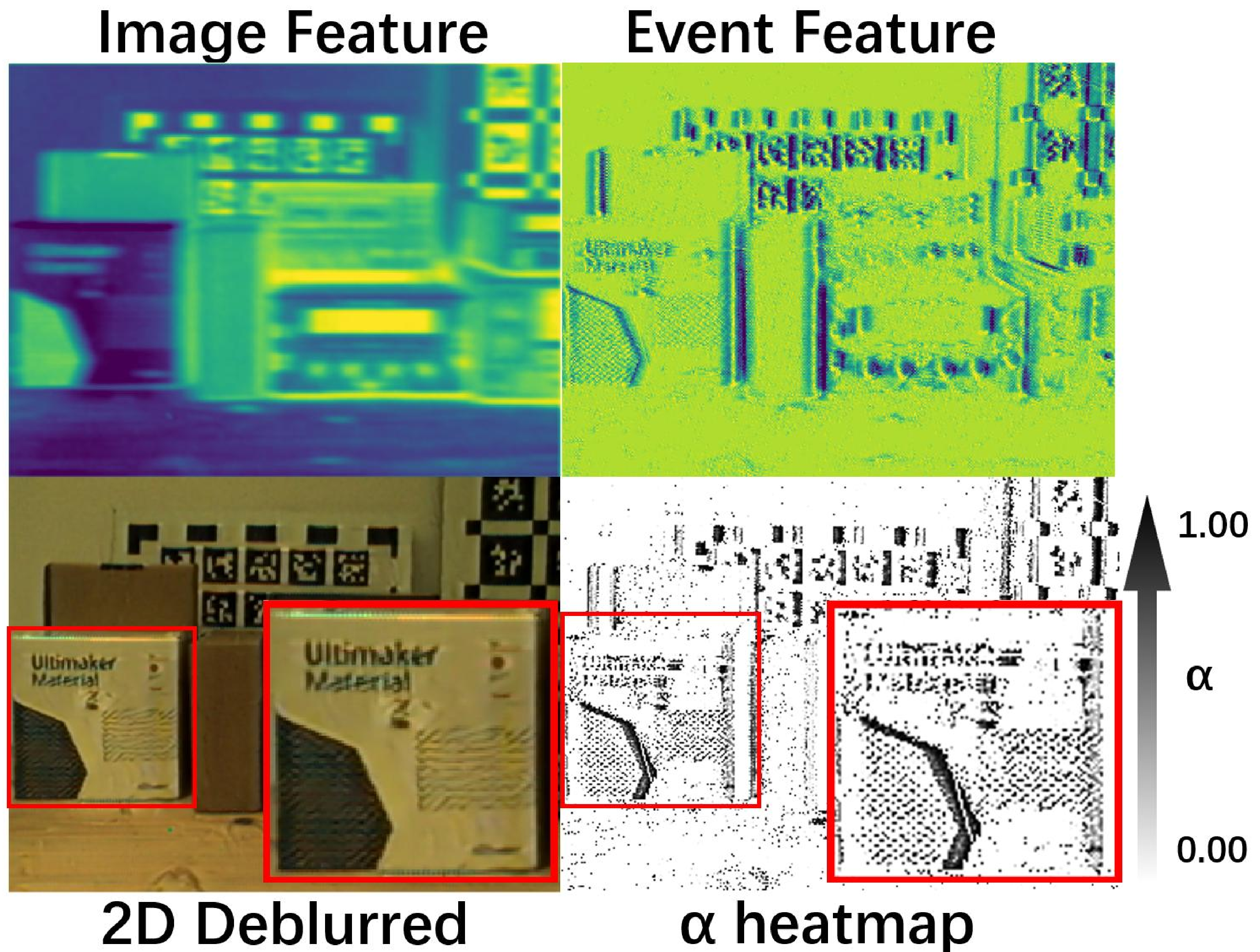
Fig. 3 relates the learned gate to scene content. Without any edge supervision, regions with strong temporal variation, motion boundaries and high-contrast edges exhibit higher event sensitivity and are routed toward the EDI reconstruction, while homogeneous or slowly varying regions fall back to the RGB observation to avoid event-integration artifacts. This content-aware split lets the loop reinforce the more reliable supervision at each location.
4.7 Qualitative Comparison↩︎
![Figure 4: Qualitative comparison on the five CDAVIS scenes (one scene per row). From left to right: blurry input, EDI+GS [10], EFNet+GS [11], DiET-GS, DiET-GS++ [28], JADE-GS (ours) and ground truth. JADE-GS matches the diffusion baselines on simple patterns (toy rocket, drones) and is sharper on complex textures (AprilTag board, porous sphere); all methods struggle on the reflective packaging box, where specular highlights create appearance ambiguity.](/article/2607.14990/figures/qualitative.png "fig:")
Fig. 4 compares JADE-GS with representative baselines on CDAVIS, with insets around toy rockets, an AprilTag board, a porous sphere, drones and reflective packaging so that local detail is visible at paper scale. Diffusion-driven baselines recover global structure but can soften or hallucinate high-contrast texture, whereas JADE-GS preserves sharper detail closer to the reference. Full five-scene breakdowns, training trajectories and additional metrics are in the supplement.
4.8 Failure Cases and Limitations↩︎
Two scenarios remain challenging. Reflective surfaces with strong specular highlights are difficult due to view-dependent appearance, an open problem in the field. Large independently moving objects violate the static-scene assumption of 3DGS, yielding inconsistent renders and unreliable backward feedback. Both weaken the 2D–3D alignment, so the method targets ego-motion blur in static scenes. Like the fixed-pose baselines, it inherits COLMAP pose errors. Pose noise, timestamp jitter, exposure mismatch, and dynamic foregrounds remain open factors that trajectory refinement [4], adaptive event-confidence weighting and dynamic Gaussian representations [35], [36] could address.
5 Conclusion↩︎
We traced the difficulty of turning events and a blurry frame into reliable 3D supervision to two coupled problems: a prior dichotomy between physics-based and learned restoration, and a coupling in which restoration and geometry never correct each other. JADE-GS resolves both, fusing the priors through a pixel-adaptive gate and closing a bidirectional loop in which detached, geometry-consistent renders and a reblurring constraint regularize the 2D restorer. Ablations isolate this coupling as the dominant factor, yielding the best perceptual quality on two public benchmarks with competitive fidelity while training in about one hour under 5 GB on a consumer GPU. Extending the loop beyond Gaussian Splatting and to dynamic scenes are natural next step
Supplementary Material for JADE-GS: Joint Alternating Deblurring Guided by Events in 3D Gaussian Splatting↩︎
6 Complementary Prior Visualization↩︎
Figure 5 illustrates the complementary behavior of the two restoration priors used by JADE-GS, motivating the fusion design in the main paper (Sec. 3.2). EDI preserves sharper boundaries but drifts and adds noise, whereas EFNet produces cleaner texture but can smooth fine structure; neither is reliable on its own, which is why the pixel-adaptive gate routes between them.
7 Per-Scene Quantitative Results↩︎
Table 3 provides the detailed per-scene evaluation on the five CDAVIS scenes. It complements the main paper by breaking down the averaged metrics across distinct scenes. JADE-GS consistently achieves top-tier results.
8 Training Trajectory Curves and Checkpoint Selection↩︎
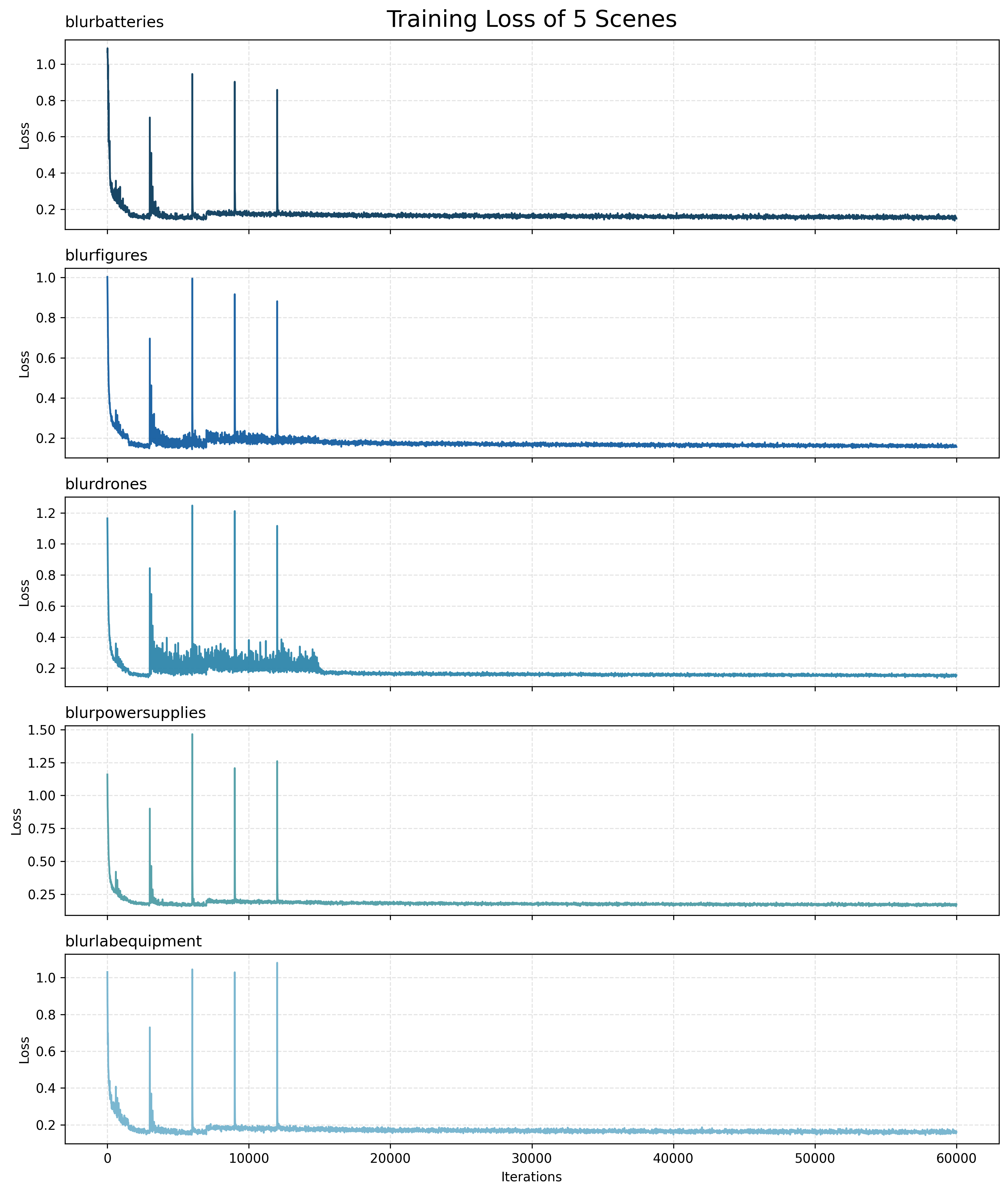
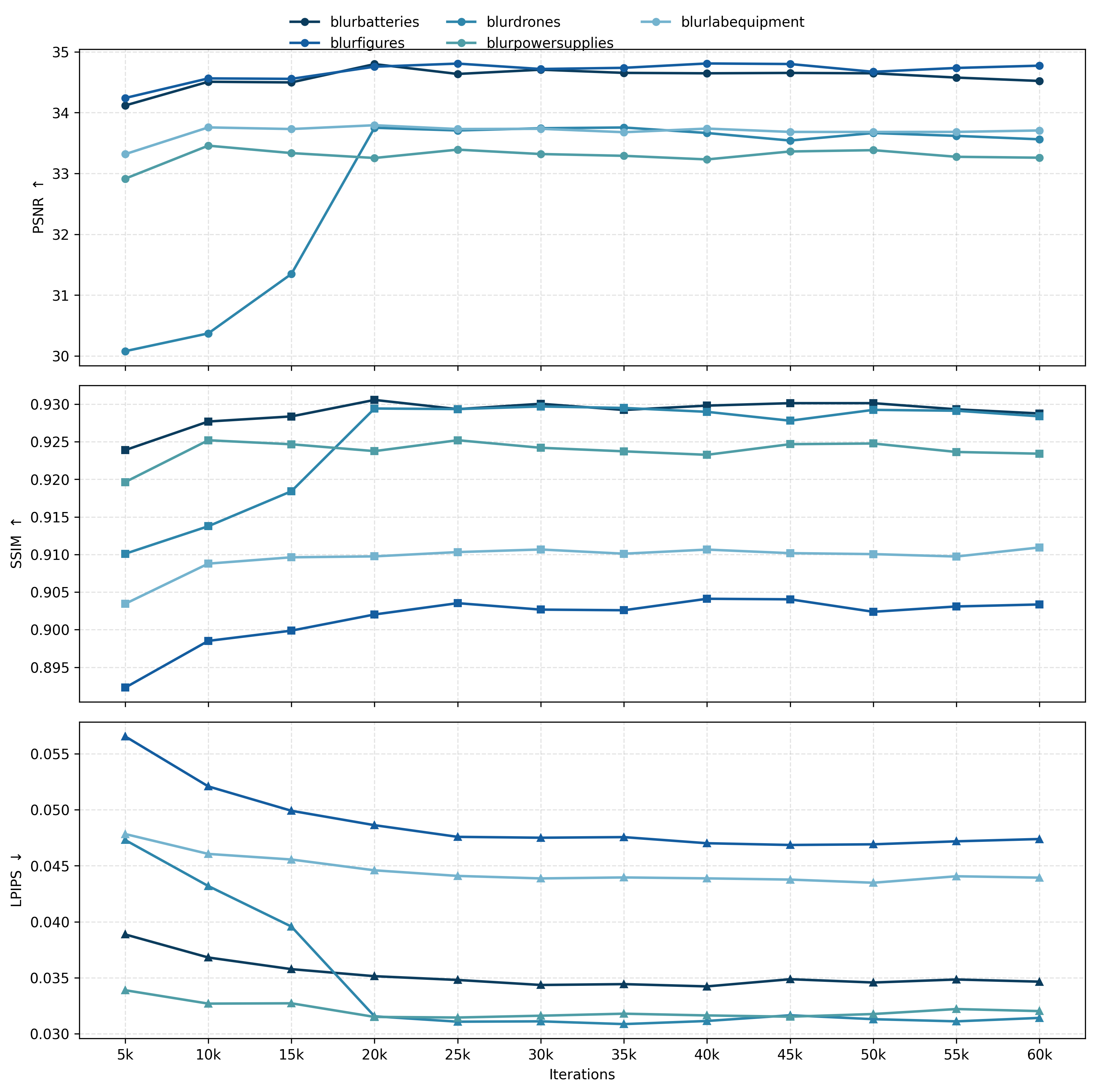
Figures 6 and 7 visualize the training loss and evaluation metrics across all five scenes. Table 4 reports PSNR, SSIM, and LPIPS at 5k-iteration intervals.
The 40k checkpoint used in the main paper is a single, scene-agnostic operating point chosen once on a held-out set of views disjoint from the evaluation views, and then applied uniformly to all scenes; training runs for 60,000 iterations. As Table 4 shows, per-scene metrics stabilize around 20k iterations and remain within a narrow band through 60k, so the 40k checkpoint captures steady-state performance rather than an oracle selection that cherry-picks each scene’s individual optimum. The advantage of JADE-GS in LPIPS therefore holds under a practical, scene-agnostic model-selection rule rather than under per-scene tuning.
9 Sensitivity to Key Hyperparameters↩︎
Table 5 evaluates three perturbed parameter configurations against the default setup (\(\lambda_{ssim}=0.1\), \(\lambda_{phy}=0.01\), \(\beta=0.1\)) on the blurbatteries scene. Across all tested directions, none of the perturbations improves over the default configuration, confirming that the chosen operating point sits near a local optimum and that the model is not sensitive to small deviations from it.
Notably, our student loss is the additive combination \(\mathrm{L1}+\lambda_{ssim}\,\mathcal{L}_{\mathrm{SSIM}}\) (Eq. 4 of the main paper) rather than the convex combination \((1-\lambda)\,\mathrm{L1}+\lambda\,\mathcal{L}_{\mathrm{D\text{-}SSIM}}\) with \(\lambda=0.2\) used by the original 3DGS, so the two weights are not directly comparable; our default \(\lambda_{ssim}=0.1\) deliberately keeps the structural term weak. It does not achieve the highest SSIM (the \(\lambda_{ssim}=1.0\) variant reaches 0.9310 versus 0.9307), but it obtains the best PSNR (34.64) and LPIPS (0.0342) simultaneously, making it the overall best operating point. This is consistent with an over-weighted structural penalty conflicting with imperfect pseudo-label supervision: forcing the student to prioritize structural fidelity amplifies artifacts from the restorer rather than the underlying scene geometry.
Although we do not ablate the two terms of \(\mathcal{L}_{tea}\) separately, the two perturbed rows probe the balance of the backward signal from complementary directions: \(\lambda_{phy}\) rescales the reblur-consistency term against the geometry-supervision term inside \(\mathcal{L}_{tea}\), while \(\beta\) rescales the backward loss as a whole against the forward loss. Over-weighting either the physical anchor (\(\lambda_{phy}\!\times\!10\)) or the backward signal overall (\(\beta\!\times\!5\)) degrades all three metrics, indicating that the default keeps geometry supervision and reblur consistency in a productive balance rather than letting either dominate.
The per-scene breakdown supports interpreting the method’s advantage primarily as a perceptual-quality and efficiency gain rather than a claim of universal dominance on every full-reference metric.
| Scene | Metric | MPRNet+GS | EDI+GS | EFNet+GS | BAD-NeRF | BAD-GS | E\(^2\)NeRF | Ev-DeblurNeRF | DiET-GS | DiET-GS++ | JADE-GS |
|---|---|---|---|---|---|---|---|---|---|---|---|
| PSNR \(\uparrow\) | 28.42 | 33.11 | 31.30 | 28.29 | 28.73 | 31.49 | 32.63 | 33.51 | |||
| SSIM \(\uparrow\) | 0.7518 | 0.8994 | 0.8556 | 0.8086 | 0.8217 | 0.8715 | 0.8938 | 0.9118 | |||
| LPIPS \(\downarrow\) | 0.1948 | 0.0613 | 0.0804 | 0.2244 | 0.1661 | 0.0932 | 0.0443 | 0.0444 | |||
| MUSIQ \(\uparrow\) | 22.13 | 37.90 | 35.51 | 17.71 | 20.20 | 37.48 | 42.99 | 45.66 | |||
| CLIP-IQA \(\uparrow\) | 0.2338 | 0.2182 | 0.2293 | 0.1887 | 0.1918 | 0.2445 | 0.2292 | 0.2327 | |||
| PSNR \(\uparrow\) | 28.18 | 33.51 | 31.28 | 29.31 | 30.12 | 32.59 | 32.82 | 33.86 | |||
| SSIM \(\uparrow\) | 0.7331 | 0.8723 | 0.8317 | 0.7703 | 0.7767 | 0.8543 | 0.8577 | 0.8846 | |||
| LPIPS \(\downarrow\) | 0.2146 | 0.0777 | 0.1324 | 0.2935 | 0.2438 | 0.1108 | 0.0687 | 0.0634 | |||
| MUSIQ \(\uparrow\) | 23.45 | 38.48 | 37.13 | 19.50 | 22.13 | 39.47 | 39.70 | 45.37 | |||
| CLIP-IQA \(\uparrow\) | 0.2415 | 0.2384 | 0.2218 | 0.1836 | 0.1898 | 0.2624 | 0.2441 | 0.2584 | |||
| PSNR \(\uparrow\) | 27.13 | 33.02 | 31.18 | 28.51 | 29.19 | 31.03 | 31.62 | 32.92 | |||
| SSIM \(\uparrow\) | 0.7634 | 0.9025 | 0.8617 | 0.8123 | 0.8317 | 0.8780 | 0.8666 | 0.9152 | |||
| LPIPS \(\downarrow\) | 0.2012 | 0.0632 | 0.1293 | 0.2122 | 0.1687 | 0.1075 | 0.0538 | 0.0396 | |||
| MUSIQ \(\uparrow\) | 28.58 | 42.55 | 41.18 | 19.05 | 22.20 | 39.00 | 41.81 | 47.58 | |||
| CLIP-IQA \(\uparrow\) | 0.1718 | 0.1633 | 0.1526 | 0.1723 | 0.1743 | 0.1887 | 0.1773 | 0.1778 | |||
| PSNR \(\uparrow\) | 26.37 | 32.10 | 30.92 | 27.53 | 28.38 | 31.06 | 32.05 | 32.37 | |||
| SSIM \(\uparrow\) | 0.7513 | 0.8955 | 0.8516 | 0.7953 | 0.8371 | 0.8820 | 0.8980 | 0.9108 | |||
| LPIPS \(\downarrow\) | 0.1828 | 0.0657 | 0.1029 | 0.2758 | 0.2247 | 0.0826 | 0.0492 | 0.0460 | |||
| MUSIQ \(\uparrow\) | 31.48 | 46.04 | 44.15 | 24.68 | 24.90 | 45.17 | 47.97 | 50.25 | |||
| CLIP-IQA \(\uparrow\) | 0.2477 | 0.2307 | 0.2219 | 0.1762 | 0.1701 | 0.2373 | 0.2510 | 0.2078 | |||
| PSNR \(\uparrow\) | 27.47 | 33.00 | 30.18 | 28.89 | 29.19 | 31.51 | 32.36 | 33.13 | |||
| SSIM \(\uparrow\) | 0.7599 | 0.8911 | 0.8512 | 0.8042 | 0.8276 | 0.8578 | 0.8772 | 0.8971 | |||
| LPIPS \(\downarrow\) | 0.2138 | 0.0871 | 0.1262 | 0.2563 | 0.2037 | 0.1355 | 0.0696 | 0.0599 | |||
| MUSIQ \(\uparrow\) | 20.18 | 35.64 | 33.18 | 18.84 | 21.19 | 32.95 | 34.14 | 40.21 | |||
| CLIP-IQA \(\uparrow\) | 0.1722 | 0.1534 | 0.1418 | 0.1749 | 0.1804 | 0.1854 | 0.1708 | 0.1958 |
3.2pt
| Scene | Metric | 5k | 10k | 15k | 20k | 25k | 30k | 35k | 40k | 45k | 50k | 55k | 60k |
|---|---|---|---|---|---|---|---|---|---|---|---|---|---|
| blurbatteries | PSNR \(\uparrow\) | 34.12 | 34.53 | 34.52 | 34.64 | 34.67 | 34.64 | 34.63 | 34.61 | 34.58 | 34.52 | ||
| SSIM \(\uparrow\) | 0.9239 | 0.9277 | 0.9284 | 0.9293 | 0.9301 | 0.9304 | 0.9305 | 0.9302 | 0.9293 | 0.9288 | |||
| LPIPS \(\downarrow\) | 0.0389 | 0.0368 | 0.0358 | 0.0351 | 0.0348 | 0.0344 | 0.0349 | 0.0346 | 0.0349 | 0.0347 | |||
| blurfigures | PSNR \(\uparrow\) | 34.24 | 34.58 | 34.61 | 34.81 | 34.75 | 34.80 | 34.84 | 34.70 | 34.71 | 34.77 | ||
| SSIM \(\uparrow\) | 0.8923 | 0.8985 | 0.8999 | 0.9020 | 0.9036 | 0.9040 | 0.9041 | 0.9042 | 0.9038 | 0.9034 | |||
| LPIPS \(\downarrow\) | 0.0566 | 0.0521 | 0.0499 | 0.0486 | 0.0476 | 0.0475 | 0.0476 | 0.0470 | 0.0472 | 0.0474 | |||
| blurdrones | PSNR \(\uparrow\) | 30.08 | 30.77 | 31.35 | 33.88 | 33.94 | 33.96 | 33.94 | 33.93 | 33.86 | 33.63 | ||
| SSIM \(\uparrow\) | 0.9111 | 0.9148 | 0.9210 | 0.9294 | 0.9299 | 0.9307 | 0.9306 | 0.9304 | 0.9299 | 0.9284 | |||
| LPIPS \(\downarrow\) | 0.0473 | 0.0432 | 0.0396 | 0.0316 | 0.0311 | 0.0311 | 0.0317 | 0.0313 | 0.0311 | 0.0314 | |||
| blurpowersupplies | PSNR \(\uparrow\) | 32.97 | 33.47 | 33.39 | 33.43 | 33.43 | 33.46 | 33.47 | 33.55 | 33.45 | 33.44 | ||
| SSIM \(\uparrow\) | 0.9196 | 0.9263 | 0.9255 | 0.9268 | 0.9252 | 0.9252 | 0.9251 | 0.9248 | 0.9249 | 0.9251 | |||
| LPIPS \(\downarrow\) | 0.0339 | 0.0327 | 0.0327 | 0.0315 | 0.0318 | 0.0316 | 0.0315 | 0.0318 | 0.0322 | 0.0320 | |||
| blurlabequipment | PSNR \(\uparrow\) | 33.48 | 33.81 | 33.83 | 33.87 | 33.84 | 33.84 | 33.82 | 33.86 | 33.83 | 33.71 | ||
| SSIM \(\uparrow\) | 0.9034 | 0.9092 | 0.9108 | 0.9115 | 0.9112 | 0.9115 | 0.9112 | 0.9116 | 0.9114 | 0.9112 | |||
| LPIPS \(\downarrow\) | 0.0478 | 0.0461 | 0.0456 | 0.0446 | 0.0441 | 0.0439 | 0.0440 | 0.0438 | 0.0441 | 0.0439 |
3.2pt
| Setting | \(\lambda_{ssim}\) | \(\lambda_{phy}\) | \(\beta\) | PSNR (\(\uparrow\)) | SSIM (\(\uparrow\)) | LPIPS (\(\downarrow\)) |
|---|---|---|---|---|---|---|
| Default Baseline | 0.1 | 0.01 | 0.1 | |||
| Stronger Physics | 0.1 | 0.1 | 0.1 | 34.42 | 0.9290 | 0.0372 |
| Stronger Backward Supervision | 0.1 | 0.01 | 0.5 | 34.49 | 0.9291 | |
| Stronger SSIM | 1.0 | 0.01 | 0.1 | 0.0383 |
3.5pt
10 Stability of the Bidirectional Loop↩︎
Because the teacher is regularized toward the student’s renders while the student fits the teacher’s targets, a natural concern is that the pair could drift toward a mutually consistent but degenerate solution. Three anchors external to the loop prevent this. First, the observed blurry frame \(B\) enters the loop twice: as the \(\alpha\!\to\!0\) fallback of the routing (Eq. 3 of the main paper) and through the reblur-consistency term (Eqs. 5–6), so the routed output is always tied to measured evidence. Second, the event stream enters through the analytic EDI branch and the EFNet conditioning, neither of which is trainable. Third, the EFNet refiner itself is frozen, so backward gradients can only re-weight the two physically grounded hypotheses at each pixel; they cannot alter the texture prior or invent content, and the trainable surface of the teacher is just the \(11{,}027\)-parameter gate. Combined with the stop-gradient on the render and the alternating update schedule (Sec. 3.5 of the main paper), this bounds how far the teacher can move toward any student artifact. Empirically, the training-loss curves in Figure 6 show stable convergence without late-stage oscillation on all five scenes, and the metric trajectories in Table 4 show no divergence through 60k iterations, consistent with a stable operating point rather than an echo chamber.
11 Training Time and Memory Comparison↩︎
Table 6 compares training efficiency across methods on the EvDeblur-CDAVIS benchmark. We report three complementary measures: total training time, training throughput (iterations per second, it/s), and peak GPU memory. Unless noted otherwise, all numbers are measured by us on a single RTX 5090; the DiET-GS row quotes the authors’ published two-stage total on a 48 GB GPU, as the method exceeds our 32 GB budget. The reported numbers are per-scene costs averaged over all five scenes. Offline (2D+GS) methods first deblur frames independently and then train 3DGS from scratch; online methods perform joint optimization. 2D+GS baselines (MPRNet+GS, EDI+GS, EFNet+GS) achieve the fastest iteration speeds (75–80 it/s) and lowest VRAM (0.5 GB) since their 2D deblurring stage is a one-time preprocess, but their low quality and lack of geometry coupling degrade final rendering accuracy. Frame-only methods trade off efficiency against fidelity: BAD-Gaussians reaches 27.6 it/s with only 2.1 GB VRAM, whereas BAD-NeRF’s per-pixel MLP sampling drops to 5.66 it/s with 15.3 GB. Event-based NeRF methods (E\(^2\)NeRF, Ev-DeblurNeRF) occupy 15.8–16.5 GB at 2.2–5.4 it/s. DiET-GS trains for close to ten hours in total across its two stages according to its authors and does not fit within a 32 GB budget. Our JADE-GS trains in 1.1 h to the reported 40k checkpoint (1.65 h for the full 60k schedule) at 10.1 it/s with 4.4 GB, roughly doubling the throughput of the NeRF baselines at about a quarter of their memory while delivering superior perceptual quality.
| EvDeblur-CDAVIS (real), \(346\times260\) | ||||
|---|---|---|---|---|
| 3-5 Method | Type | Time (h)\(\downarrow\) | Speed (it/s)\(\uparrow\) | VRAM (GB)\(\downarrow\) |
| MPRNet+GS | 2D+GS | \(\sim\)0.5 h | 75\(\sim\)80 | 0.5 |
| EDI+GS | 2D+GS | \(\sim\)0.5 h | 75\(\sim\)80 | 0.5 |
| EFNet+GS | 2D+GS | \(\sim\)0.5 h | 75\(\sim\)80 | 0.5 |
| BAD-NeRF | frame | \(\sim\)10 h | 5.66 | 15.3 |
| BAD-Gaussians | frame | \(\sim\)0.5 h | 27.6 | 2.1 |
| E\(^2\)NeRF | event | \(\sim\)10 h | 5.4 | 16.5 |
| Ev-DeblurNeRF | event | \(\sim\)6 h | 2.2 | 15.8 |
| DiET-GS\(^\dagger\) (stages 1+2) | event | \(\sim\)10 h | – | OOM (\(>\)32) |
| JADE-GS (ours) | event | 1.1 h\(^{\ast}\) | 10.1 | 4.4 |
1.8pt