CFM-Bench: A Unified Multi-Domain, Multi-Task Benchmark for Channel Foundation Models
July 16, 2026
Abstract
Channel foundation models (CFMs) are developing rapidly, with recent studies reporting benefits from pretraining across downstream wireless tasks. Yet CFMs are commonly evaluated in model-specific pipelines with different data, radio configurations, partitions, adaptation procedures, task definitions, and metrics. Reported comparisons therefore tend to show that pretraining improves over supervised training from scratch within one pipeline, but neither rank CFMs nor compare them fairly with task-specific models. We release CFM-Bench, a unified multi-domain, multi-task benchmark designed to address this gap. It curates six channel configurations spanning 3GPP statistical simulation, two independent ray-tracing pipelines, industrial and aerial measurements, and synchronized vehicular multimodal simulation. Official partitions isolate complete trajectories, measurement sessions, vehicle links, simulation realizations, or buffered spatial regions. CFM-Bench does not prescribe an external pretraining corpus or strategy; no benchmark split may be used for foundation-model pretraining, and the official training split is reserved exclusively for downstream fine-tuning. The benchmark additionally requires disclosure of all data used during model development and prohibits training-stage use of official test units. Six task groups are organized along three CFM application dimensions: physical-layer (PHY) channel intelligence, radio-access-network (RAN) decision intelligence, and integrated sensing and communication (ISAC). They cover CSI feedback, frequency and temporal channel extrapolation, propagation-state classification, current- and future-beam prediction, and single-frame and temporal localization. CFM-Bench provides a common substrate for comparing the transferability of channel representations across models, domains, and tasks.
Channel foundation model, channel state information, benchmark, multi-domain learning, multi-task learning, wireless artificial intelligence, transfer learning.
1 Introduction↩︎
Artificial intelligence (AI) is shifting from a supporting tool for network tuning into a native element of the wireless air interface. The 3rd Generation Partnership Project (3GPP) has examined how AI/machine-learning functions can fit into New Radio (NR), covering data gathering, model training, adaptation, inference, and lifecycle management [1], [2]. At the same time, foundation models have shown that a single pretrained representation can serve many downstream tasks after light adaptation [3]. When this idea is applied to wireless channels, it points toward channel foundation models (CFMs) that extract reusable representations from channel state information (CSI), impulse responses, geometry, and surrounding context [4].
Work on CFMs is advancing quickly. Recent studies rely on masked reconstruction, autoencoder, and other self-supervised goals to handle reconstruction, prediction, and related channel problems [5]–[7]. Most of the supporting evidence, however, comes from isolated pipelines: each study trains a model from scratch on its own data and protocol, then compares the pretrained version against that same baseline. Because the pretraining sets, radio settings, data splits, task definitions, adaptation budgets, and scoring rules vary from one paper to the next, the published numbers do not reveal which model transfers more effectively or whether a general-purpose CFM actually outperforms a task-specific architecture under matched conditions.
Existing studies on evaluating channel foundation models exhibit three notable limitations. First, although some works conduct cross-CFM comparisons within individual papers, these comparisons are typically performed under disparate pretraining corpora, system configurations, data partitioning schemes, task definitions, and evaluation metrics. As a result, the field still lacks a unified evaluation protocol, making it difficult to establish community-wide consensus on the relative transferability of different models or to determine whether general-purpose channel representations genuinely outperform task-specific architectures. Second, most existing efforts rely on a single channel generation mechanism for both training and evaluation, whether based on 3GPP statistical models or specific ray-tracing environments. This restricts the ability to systematically test models across diverse propagation physics, including stochastic variation, geometry-consistent multipath, hardware-induced effects, and environmental sensing information. While simulation datasets offer scalability, the performance gap between simulated and measured channels remains insufficiently characterized without broader mechanism coverage. Third, wireless channels exhibit strong spatio-temporal correlation, with samples from the same trajectory or measurement session sharing highly similar multipath structures, angles, and delays. Many prior works employ random frame-level splitting for training and test sets, which introduces substantial information overlap between the two. This practice systematically inflates reported performance metrics and masks overfitting, leading to overly optimistic assessments of generalization capability. Although some recent studies have adopted trajectory- or session-level partitioning, such practices have not yet become standard, and systematic validation across datasets remains limited.
A meaningful benchmark must therefore go beyond reporting isolated test scores. It must prevent pretraining leakage, publish stable downstream partitions, and require transparent reporting of the data used during model development. It must also span complementary channel mechanisms so that learned representations can be evaluated for robustness across statistical variation, geometry-consistent multipath, hardware effects, and multimodal context. The release should preserve physical metadata while allowing each model to choose its own input representation and preprocessing.
CFM-Bench addresses these needs by curating one representative configuration from each of six data sources and imposing a common release and evaluation contract. The benchmark contains a 3GPP urban microcell statistical domain, a Wireless InSite-based 60-GHz urban ray-tracing domain, a Sionna-based ten-base-station campus domain, two measured massive-MIMO domains, and a synchronized vehicular multimodal domain. Source-specific data interfaces retain the available channel and physical metadata without prescribing a fixed model input shape. Official partitions, task definitions, metrics, and a test-exposure policy make the release a common comparison substrate rather than another model-specific evaluation dataset. Its six task groups span physical-layer (PHY), radio access network (RAN), and integrated sensing and communication (ISAC) applications.
The main contributions are as follows.
We release a unified multi-domain, multi-task benchmark built for reproducible comparison of CFMs against each other and against task-specific networks. The six domains together cover statistical, deterministic, measured, and multimodal channels in indoor, outdoor, terrestrial, and aerial settings.
We supply source-specific data interfaces that preserve complex CSI, frequency and array geometry, mobility information, base-station context, and synchronized sensing streams. Each team remains free to choose its own resampling, normalization, and tokenization steps, provided these choices are reported.
We define leakage-resistant partitions that respect complete trajectories, measurement sessions, vehicle links, random-seed groups, or buffered spatial regions. A required data-exposure statement together with a strict test-isolation rule ensures that any model that touched an official test unit during development cannot be presented as a compliant result.
We define six task groups spanning PHY, RAN, and ISAC applications, including an end-to-end CSI-feedback reconstruction protocol with NMSE as the primary metric and SGCS as the secondary similarity metric. Dataset-specific beam candidate spaces, physical prediction horizons, validity masks, native localization frames, and metrics prevent superficially similar labels from being compared under incompatible semantics.
We audit numerical validity, temporal continuity, beam-label reproducibility, coordinate precision, and multimodal leakage. The resulting task-support matrix disables scientifically unsupported combinations instead of manufacturing labels for every domain.
The remainder of the paper is organized as follows. Section 2 reviews channel datasets and CFMs. Section 3 introduces the benchmark scope and access rules. Section 4 describes the six domains and data access. Section 5 defines test isolation and the PHY, RAN, and ISAC tasks. Sections 6 and 7 discuss data availability and limitations, followed by the conclusion in Section 8.
2 Related Work↩︎
2.1 Channel Datasets and Generation Platforms↩︎
DeepMIMO introduced a configurable interface for generating massive-MIMO channels from ray-tracing scenarios, enabling reproducible learning studies on spatially consistent channels [8]. Sionna and Sionna RT later offered open, differentiable tools for physical-layer simulation and radio propagation [9], [10]. These platforms allow large-scale channel generation, yet dependence on a single simulator can tie model performance to simulator-specific geometry, material assumptions, and data formatting conventions.
Several public datasets complement these platforms. MOCSID supplies Sionna-RT-generated pedestrian trajectories under overlapping coverage from ten outdoor base stations [11], [12]. DICHASUS provides phase-coherent measured massive-MIMO channels together with accurate position labels; its ADXX release records a distributed 64-antenna deployment in an industrial setting [13], [14]. The MaMIMO-UAV campaign captures wideband air-to-ground channels between an \(8\times8\) base-station array and a moving UAV [15], [16]. Multimodal-Wireless aligns ray-traced CSI with camera, depth, LiDAR, radar, inertial, and positioning data inside CARLA environments [17]. Each resource serves its original purpose well. CFM-Bench retains the provenance of these sources while adding shared partitions and task protocols that enable cross-domain evaluation.
2.2 Channel Foundation Models↩︎
Current CFM studies can be grouped into two broad methodological lines [4]. One line focuses on learning reusable representations from unlabeled channel observations. LWM employs masked channel modeling to pretrain a task-agnostic feature extractor [5]. WiFo learns transferable space–time–frequency structure specifically for channel prediction [6]. CSI-MAE extends masked autoencoding to support both channel perception and generation tasks [7]. CSI-CLIP++ aligns frequency-domain CSI with its delay-domain impulse response through contrastive pretraining, targeting channel identification, beam prediction, and positioning [18]. Filter-and-Attend instead emphasizes robustness when observed CSI is corrupted by noise and interference [19].
A second line expands the task or system-configuration scope of a single pretrained model. The wireless multi-task model in [20] jointly handles CSI, location, and traffic prediction within a unified sequence formulation. WiFo-E targets end-to-end frequency-division-duplex precoding and employs sparse mixture-of-experts routing to accommodate varying antenna and user configurations [21]. These approaches reduce the need for a separate network at every operating point, yet their downstream protocols remain closely tied to the individual model and application.
Together, these studies illustrate the promise of reusable channel representations and task- and configuration-aware adaptation. Their reported results, however, remain difficult to compare directly. Pretraining corpora, channel representations, available modalities, data partitions, adaptation budgets, target definitions, and evaluation metrics differ across works. CFM-Bench complements ongoing model development by supplying a fixed evaluation substrate, enforcing test-unit isolation, and requiring full disclosure of pretraining and adaptation data. In this way it enables transfer assessment under matched downstream conditions without prescribing any particular CFM architecture or pretraining objective.
3 CFM-Bench Overview↩︎
3.1 Scope and Design Choices↩︎
Each source contributes one fixed combination of environment, carrier, bandwidth, array geometry, and acquisition procedure. Within that configuration, CFM-Bench retains multiple trajectories or sessions because they serve as independent partition units. Alternative towns, carrier frequencies, weather conditions, or array variants from the same source are excluded. This choice broadens mechanism-level diversity while preventing any single source from dominating the benchmark through many closely related configurations.
CFM-Bench treats differences in antenna layout, bandwidth, frequency grid, and sampling rate as an explicit evaluation dimension rather than a source of inconsistency. Source-aware data interfaces preserve the corresponding physical metadata, while each model remains free to apply its own input transformations. These choices must be documented with the reported results.
3.2 Partition and Training Access↩︎
Wireless channel samples are strongly correlated across time and space. Random frame-level splitting therefore risks placing nearly identical channels into both training and test sets. To avoid this, CFM-Bench partitions at the level of the largest available independent unit: a complete trajectory or simulation realization, a measurement session, a full vehicle link, or a buffered spatial region. When a source supplies enough comparable units, an 8:1:1 allocation is applied. When only a few units are available, validation and test each receive one distinct held-out unit, and the leakage boundary is defined by the entire trajectory, session, flight, or link.
Training, validation, and test data are all released, yet their permitted uses differ. No CFM-Bench split may be included in foundation-model pretraining. The official training data are reserved exclusively for downstream fine-tuning under the declared task protocol. Validation data may guide model selection and hyperparameter tuning but may not be used for parameter updates. Test units are reserved exclusively for final inference and scoring; they may not influence model development in any way. The benchmark does not rely on a hidden evaluation server. Reproducibility is instead ensured through fixed split definitions, validation checks, and mandatory disclosure of all data used during model development.
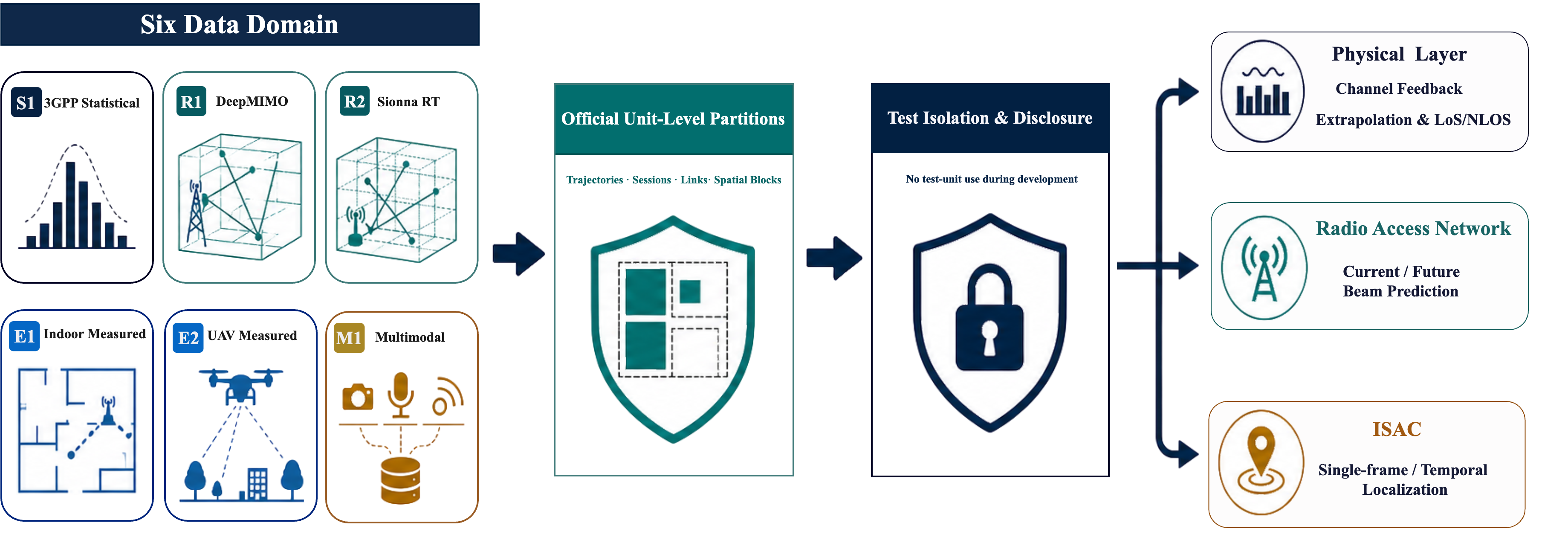
Fig. 1 illustrates the overall benchmark flow: heterogeneous sources are processed through official partitions and test-isolation rules before feeding into the three CFM application dimensions.
4 Dataset Composition↩︎
Table 1 summarizes the six radio configurations. The identifiers encode provenance rather than quality: S denotes statistical simulation, R ray tracing, E a measured environment, and M synchronized multimodal simulation. Counts refer to the official single-frame view; temporal windows are reported separately.
| ID | Data source | Mechanism | Scenario | ||
| bandwidth | Released CSI view | ||||
| S1 | 3GPP TR 38.901 UMi | Statistical (Sionna) | Three-site urban microcell | 3.5 GHz / 100 MHz | 9 links; 64 BS ports; 128 tones |
| R1 | DeepMIMO O1_60 | RT (Wireless InSite) | Outdoor urban grid | 60 GHz / 400 MHz | 64 BS ports; 256 tones |
| R2 | MOCSID | RT (Sionna) | Campus; 10 BSs; pedestrians | Unspecified / 1.92 MHz | 10 BS links; 64 tones on a 30-kHz grid |
| E1 | DICHASUS ADXX | Measurement | Industrial indoor | 3.440 GHz / 50.056 MHz | 64 distributed antennas; 1024 tones |
| E2 | MaMIMO-UAV | Measurement | Outdoor air-to-ground | 2.61 GHz / 18 MHz | 64 BS elements; 100 tones |
| M1 | Multimodal-Wireless | Multimodal RT | Town05 CBD V2I | 28 GHz / narrowband | \(16\times64\) RSU–vehicle channel matrix |
3.8pt
4.1 Dataset Scale and Diversity↩︎
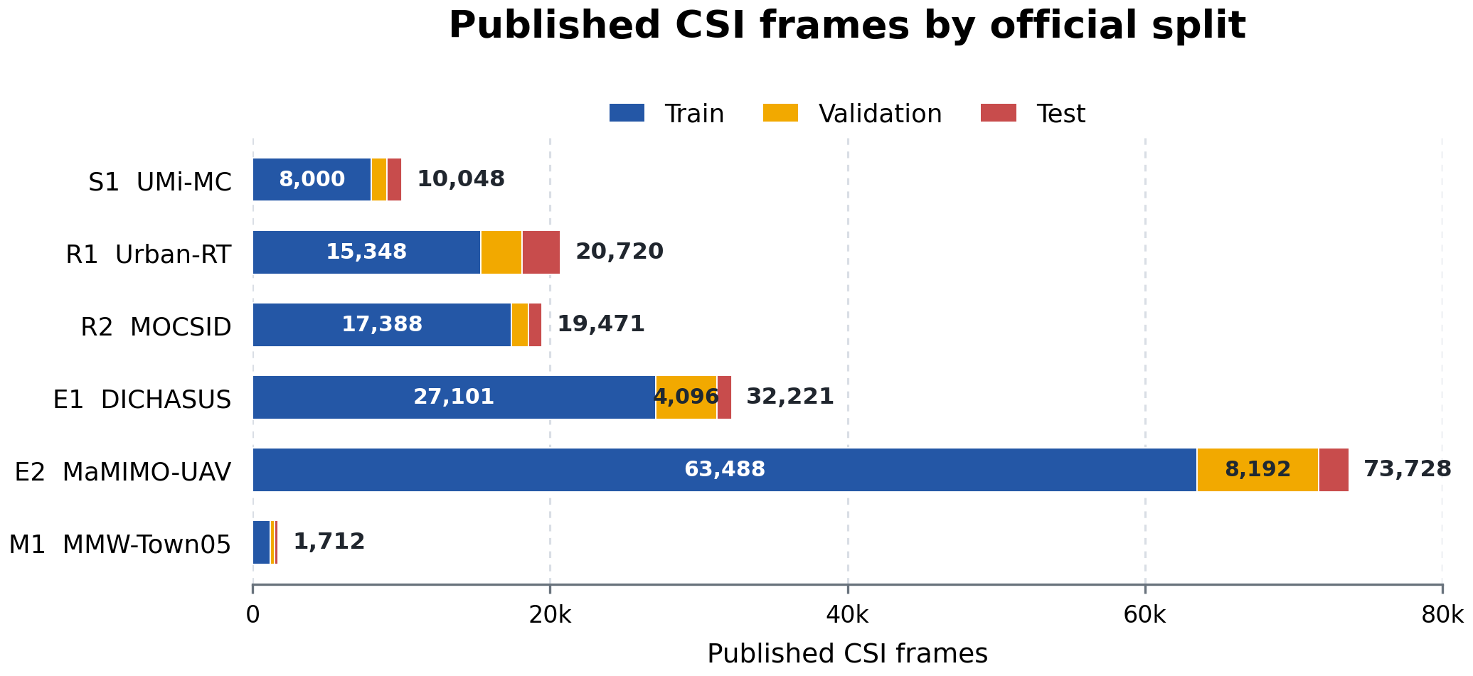
CFM-Bench contains 157,900 single-frame examples: 132,525 for training, 17,523 for validation, and 7,852 for testing. Fig. 2 reports these counts by domain and split. The per-domain totals are 10,048 for S1, 20,720 for R1, 19,471 for R2, 32,221 for E1, 73,728 for E2, and 1,712 for M1. The counts refer to benchmark examples retained after quality control and source-specific sampling, rather than every sample in the original datasets. The imbalance is intentional: CFM-Bench preserves independent physical units and reports per-domain scores instead of forcing every source to an arbitrary common size. Temporal windows provide alternative evaluation views of test sequences and are not added to the single-frame totals.
Table ¿tbl:tab:task95support? shows broad coverage without claiming that every target is physically meaningful for every source. CSI feedback creates protocol-defined observations from the released complex CSI and is available in all six domains. Frequency extrapolation is available in the five wideband domains, whereas complex temporal extrapolation is restricted to R2 and M1. E1 retains uncompensated measurement phase and E2 does not release a complete future-CSI target view, so neither is included in that task. Current-beam prediction is enabled for S1, R1, R2, E1, and E2, while future-beam prediction is enabled for R2, E1, and E2. M1 provides no official current- or future-beam target. LoS/NLoS supervision is restricted to S1 and R2, and single-frame localization covers all six domains.
3.0pt
@c *8Z@ & & &
(lr)2-5(lr)6-7(lr)8-9 Domain & & & & & & & &
S1 3GPP UMi & & & & & & & &
R1 DeepMIMO & & & & & & & &
R2 MOCSID & & & & & & & &
E1 DICHASUS & & & & & & & &
E2 MaMIMO-UAV & & & & & & & &
M1 Multimodal & & & & & & & &
The diversity attributes in Table ¿tbl:tab:diversity? complement raw sample count with mechanism and context coverage. The benchmark includes one 3GPP statistical domain, three ray-tracing-based domains, and two measured domains. The deployment settings cover indoor industrial, terrestrial outdoor, aerial, and vehicular links. Four domains preserve temporal sequences; S1 and R2 expose multiple base stations, E1 uses distributed receiving sites, E2 and M1 provide three-dimensional positions, and M1 adds synchronized environmental sensing. The benchmark therefore varies both channel generation and the physical context paired with each observation.
2.6pt
@c *11Z@ & & &
(lr)2-4(lr)5-8(lr)9-12 Domain & Stat. & RT & Meas. & Indoor & & Aerial &
V2I & Temporal & & & Sensors
S1 3GPP UMi & & & & & & & & & & &
R1 DeepMIMO & & & & & & & & & & &
R2 MOCSID & & & & & & & & & & &
E1 DICHASUS & & & & & & & & & & &
E2 MaMIMO-UAV & & & & & & & & & & &
M1 Multimodal & & & & & & & & & & &
4.2 Statistical and Ray-Traced Domains↩︎
S1: 3GPP urban microcell. S1 follows the 3GPP TR 38.901 urban-micro street-canyon model [22], implemented in Sionna with three sites and three sectors per site. Each sector uses an \(8\times8\) uniform rectangular array (URA), while the user equipment (UE) has one antenna. The dataset contains 8,000 training, 1,024 validation, and 1,024 test snapshots drawn from mutually disjoint simulation realizations and UE routes. It is treated as static because independently generated channel segments do not provide physically continuous complex CSI. S1 therefore supports frequency extrapolation, LoS/NLoS classification, per-valid-sector current-beam prediction, and single-frame localization, but no temporal task. Each observation retains nine sector links and their validity mask; this is a multi-link tensor, not a single 576-port array.
R1: DeepMIMO O1_60. R1 uses the 60-GHz DeepMIMO O1_60 outdoor scenario, whose site-specific propagation paths were generated with Remcom Wireless InSite [8]. It contains a static two-dimensional user grid, an \(8\times8\) base-station URA, and 256 subcarriers over 400 MHz. One of every 50 spatial samples is retained after partitioning to keep the benchmark size tractable. The coverage area is divided into ten non-overlapping regions, with 1-m guard bands preventing adjacent grid points from crossing split boundaries. Samples with no valid ray-traced path are removed. LoS/NLoS classification is not an official R1 task because its held-out regions contain only NLoS examples.
R2: MOCSID. MOCSID models an outdoor campus with ten base stations, overlapping coverage, mixed line-of-sight (LoS) and non-LoS propagation, and spatially consistent pedestrian mobility [11], [12]. CFM-Bench selects ten complete trajectories while retaining their temporal samples, visible-base-station information, and positions. Frequency-domain CSI is derived from the released path coefficients and delays on an explicitly benchmark-defined 64-tone, 30-kHz relative baseband grid; it is not presented as an upstream OFDM configuration. The per-BS LoS/NLoS labels are geometry-derived and use a link-valid mask. Eight trajectories form the training set, and one trajectory is assigned to each evaluation split.
4.3 Measured Channel Domains↩︎
E1: DICHASUS ADXX. CFM-Bench uses the public DICHASUS ADXX dataset recorded in the ARENA2036 facility [13], [14]. The source specifies a 3.440-GHz carrier, 50.056-MHz bandwidth, 1024 subcarriers, 64 antennas arranged as four distributed \(2\times8\) arrays, and a 48-ms measurement interval. Upstream reference-channel phase/time compensation is not applied in the release. Consequently, beamforming is performed only within each physical array and raw complex temporal CSI extrapolation is disabled, while magnitude-robust future-beam prediction and temporal localization remain supported. Two sessions are assigned to training, and distinct sessions define validation and test; retained windows never cross acquisition gaps.
E2: MaMIMO-UAV. E2 captures a measured air-to-ground channel between a 64-element upward-facing URA and a UAV following three-dimensional trajectories [15], [16]. It retains the 2.61-GHz carrier, 18-MHz occupied bandwidth, 100 subcarriers, 1-ms sampling interval, and flight metadata. Two all-zero acquisition segments are removed. Geographic coordinates are interpolated in double precision before conversion to local east–north metres, eliminating quantization steps that would otherwise corrupt millisecond-scale motion. Four flights are assigned to training and one each to validation and test. Complex temporal CSI extrapolation is disabled, but future-beam prediction and temporal localization remain supported on continuity-safe segments.
4.4 Synchronized Multimodal Domain↩︎
M1: Multimodal-Wireless. Multimodal-Wireless uses CARLA and Sionna to pair CSI with environmental sensing [17]. CFM-Bench uses the Town05 CBD Crossroad under sunny weather and a 28-GHz vehicle-to-infrastructure link. The narrowband \(16\times64\) CSI is aligned at 100 Hz with four vehicle-mounted RGB cameras, LiDAR, and inertial records. Three distinct vehicle links define the training, validation, and test partitions, containing 1,200, 256, and 256 retained frames, respectively. Pose, GPS, and sensor world-coordinate fields are target metadata and are forbidden as localization inputs; a localization method may use CSI, RGB, LiDAR, and inertial measurements that do not reveal absolute pose. This protocol tests unseen-link transfer within one scene, not transfer across towns or weather.
4.5 Partition Summary↩︎
Table 2 jointly reports dataset scale and the unit of independence. Each dataset row gives single-frame examples followed by the number of source isolation units; the total row sums frames only. Any subset used for downstream fine-tuning must be drawn only from the listed training units and reported with the evaluation; benchmark examples must never enter foundation-model pretraining. The temporal test views contain 64 windows of length 32 for E1, 64 of length 64 for E2, 8 of length 32 for R2, and 16 of length 16 for M1. These windows remain within their respective held-out source units and do not change the single-frame counts.
| ID | Partition unit | Train | Validation | Test | Isolation rule |
|---|---|---|---|---|---|
| S1 | Simulation realization | 8,000 / 16 | 1,024 / 2 | 1,024 / 2 | Disjoint random seeds and UE routes |
| R1 | Spatial region | 15,348 / 8 | 2,780 / 1 | 2,592 / 1 | 1-m guard bands between splits |
| R2 | Pedestrian trajectory | 17,388 / 8 | 1,175 / 1 | 908 / 1 | Each trajectory belongs to one split |
| E1 | Measurement session | 27,101 / 2 | 4,096 / 1 | 1,024 / 1 | No source session crosses a split |
| E2 | UAV flight | 63,488 / 4 | 8,192 / 1 | 2,048 / 1 | No source flight crosses a split |
| M1 | Vehicle link | 1,200 / 1 | 256 / 1 | 256 / 1 | No source vehicle link crosses a split |
| All | – | 132,525 | 17,523 | 7,852 | 157,900 frames in total |
3.6pt
4.6 Data Format and Access↩︎
CFM-Bench preserves source-specific CSI structures rather than requiring every domain to share a fixed model input shape. Each example includes complex CSI and the task annotations and physical metadata that are meaningful for its source, such as frequency coordinates, array information, timestamps, positions, base-station identities, and synchronized sensing modalities. The dataset documentation specifies the representation and units for each domain.
Dynamic examples preserve timestamp order, and a temporal window never crosses a trajectory, session, flight, vehicle-link, acquisition gap, or retained-segment boundary. The sensing streams in M1 retain their original frame alignment. Task-specific input restrictions prevent target-bearing position information from being used for localization. Resampling, antenna selection, normalization, padding, and tokenization are model-specific choices and must be documented; any fitted preprocessing statistics must use training data only.
4.7 Quality Control and Task Eligibility↩︎
The data are audited at both numerical and semantic levels. Every retained CSI tensor is finite and contains nonzero energy; all-zero R1 spatial samples and two all-zero E2 acquisition segments are removed. R2 may contain an all-zero channel for an individual unavailable BS, but such a link is retained only when it matches the corresponding validity mask. An unavailable link is excluded from link-specific losses and metrics without discarding a frame whose other BS links remain meaningful. Beam labels are recomputed from the CSI and codebooks, and position labels are checked for finite values, units, coordinate references, and continuity within every temporal segment.
Task eligibility follows the data-generating semantics rather than the presence of a convenient tensor axis. S1 is treated as static snapshots because independently generated channel segments do not constitute continuous complex CSI. R1 is a spatial grid rather than a time series. E1 does not expose uncompensated raw complex CSI as a temporal-extrapolation task, and E2 does not provide complete future-CSI supervision. M1 is narrowband and therefore does not support frequency extrapolation. These exclusions do not invalidate other tasks derived from the same observations.
5 Benchmark Tasks and Evaluation Protocol↩︎
5.1 Evaluation Fairness and Data-Exposure Policy↩︎
CFM-Bench does not prescribe an external pretraining corpus, objective, model architecture, or fine-tuning strategy. A compliant evaluation must keep every CFM-Bench example out of foundation-model pretraining. Only the official training split may be used for downstream fine-tuning. Validation data may be used for model and hyperparameter selection but not for parameter updates or merged into the training data. Test trajectories, measurement sessions, vehicle links, spatial blocks, and simulator groups, together with any samples derived from them, may not be used for fine-tuning, normalization-statistics estimation, model selection, or data augmentation. Test inputs are accessed only for final inference, and test labels are used only for scoring.
Every reported result must include a data-exposure statement listing all CFM-Bench and external data used during model development. For external pretraining data, the statement identifies any overlapping map, site, measurement campaign, simulator scene, trajectory, flight, session, or vehicle link. Pretraining on any CFM-Bench example violates the protocol and disqualifies the result from standard ranking. Use of an official test unit or any unpublished sample from that unit during model development is additionally labeled test-exposed or transductive. Because several domains hold out trajectories, sessions, links, or spatial regions within a shared broader environment, CFM-Bench guarantees unit-level isolation rather than universal scene-level isolation. M1, for example, evaluates an unseen vehicle link within the same Town05 run. Additional exposure to a test environment must therefore be disclosed and considered when comparing results.
When a comparative claim is made between a CFM and a task-specific model, both models must use the same allowed observations and modalities, training examples, validation and test units, and target definition. Parameter count and inference cost must accompany the comparison, and training compute is reported when available. Each submission reports per-domain scores; an unweighted macro-average across eligible domains is only a secondary summary.
5.2 Common Metric Conventions↩︎
Let \(\mathcal{V}_i\) denote the valid target entries for sample \(i\) after applying validity and task masks, and let \(\mathbf{h}_i\) and \(\widehat{\mathbf{h}}_i\) be vectorized complex targets and predictions on \(\mathcal{V}_i\). Zero-energy targets are excluded and counted in the evaluation log. The aggregate normalized mean-squared error in decibels is \[\mathop{\mathrm{NMSE}}_{\mathrm{dB}}=10\log_{10} \frac{\sum_i\|\widehat{\mathbf{h}}_i-\mathbf{h}_i\|_2^2}{\sum_i\|\mathbf{h}_i\|_2^2}. \label{eq:nmse}\tag{1}\] The squared generalized cosine similarity is \[\mathop{\mathrm{SGCS}}=\frac{1}{N}\sum_{i=1}^{N} \frac{|\mathbf{h}_i^{H}\widehat{\mathbf{h}}_i|^2}{\|\mathbf{h}_i\|_2^2\|\widehat{\mathbf{h}}_i\|_2^2}. \label{eq:sgcs}\tag{2}\] NMSE measures complex reconstruction or extrapolation fidelity, whereas SGCS measures directional agreement relevant to spatial processing. Both are common in CSI learning studies [23].
Table 3 summarizes the taxonomy, eligible domains, targets, and primary evaluation metrics of the six official task groups. Channel extrapolation and localization each expose two evaluation variants, producing the eight support columns in Table ¿tbl:tab:task95support?; detailed observation budgets and secondary metrics are defined below. An unsupported domain–task combination is omitted rather than assigned a synthetic label.
| Dim. | Task | Eligible domains | Prediction target | Primary metric |
|---|---|---|---|---|
| CSI feedback | All six domains | Full CSI from a compressed latent representation | NMSE (dB) | |
| Channel extrapolation | Frequency: S1, R1, R2, E1, E2; temporal: R2, M1 | Missing-frequency or future CSI | Target-only NMSE (dB) | |
| LoS/NLoS classification | S1, R2 | Binary state of each valid link | Macro-F1 | |
| Current-beam prediction | S1, R1, R2, E1, E2 | Current codebook-defined beam or beam pair | Top-1/Top-3 accuracy | |
| Future-beam prediction | R2, E1, E2 | Future codebook-defined beam or beam pair | Horizon-wise Top-1/Top-3 accuracy | |
| Localization | Single frame: all; temporal: R2, E1, E2, M1 | Native-frame Cartesian position in metres | Mean 3D error (m) |
4.0pt
5.3 PHY↩︎
CSI feedback: Accurate downlink CSI at the base station (BS) is essential for precoding, beamforming, scheduling, and link adaptation. In frequency-division-duplex massive-MIMO systems, uplink and downlink channels are not directly reciprocal, so the user equipment (UE) must convey a compact representation of its estimated downlink CSI to the BS. Learning-based feedback addresses the resulting dimensionality challenge by jointly training a UE-side encoder and a BS-side decoder, while practical comparisons must also account for encoder complexity, generalization, and encoder–decoder interoperability [24]. CSI feedback enhancement is also a representative two-sided air-interface AI/ML use case studied in 3GPP TR 38.843, where CSI is compressed at the UE and reconstructed at the BS within the legacy feedback framework [25], [26].
For sample \(i\), let \(\mathbf{h}_i\in\mathbb{C}^{D_i}\) contain the released complex CSI coefficients selected by the domain validity mask, and let \(\mathbf{x}_i=[\operatorname{Re}(\mathbf{h}_i)^{T},\operatorname{Im}(\mathbf{h}_i)^{T}]^{T}\in\mathbb{R}^{2D_i}\) be their real-valued representation. The encoder \(f_{\boldsymbol{\theta}}(\cdot)\) maps \(\mathbf{x}_i\) to an \(M_i\)-dimensional latent representation, and the decoder \(g_{\boldsymbol{\phi}}(\cdot)\) reconstructs it: \[\mathbf{z}_i=f_{\boldsymbol{\theta}}(\mathbf{x}_i),\qquad \widehat{\mathbf{x}}_i=g_{\boldsymbol{\phi}}(\mathbf{z}_i).\] The dimensional compression ratio is \(\gamma_i=M_i/(2D_i)\). Comparisons within a domain must use the same declared \(\gamma_i\) and the same valid CSI coefficients. The reconstructed real and imaginary components form \(\widehat{\mathbf{h}}_i\). The primary metric is aggregate NMSE in decibels as defined in 1 ; lower values indicate more accurate CSI reconstruction. SGCS in 2 is secondary and measures preservation of the complex channel direction, with values closer to one indicating stronger similarity. These complementary error and similarity measures are commonly used for CSI feedback and are considered in 3GPP TR 38.843 [24], [25].
Channel extrapolation: Channel extrapolation involves predicting wireless channel states in new or unseen domains, such as extending limited pilot-based CSI measurements across frequency, time, or space, to support more efficient beamforming and resource management in dynamic 6G environments [27]–[29]. Let \(\mathbf{H}\) denote the complex channel representation supplied by an eligible domain. In frequency extrapolation, the official index arrays divide the valid subcarriers into central observed bins \(\Omega_{\mathrm{obs}}\) and outer target bins \(\Omega_{\mathrm{tar}}\). The model receives \[\mathbf{H}_{\mathrm{obs}}=\mathbf{M}_{\mathrm{obs}}\odot\mathbf{H}\] together with the indices and allowed physical metadata, and predicts only \(\Omega_{\mathrm{tar}}\). M1 is excluded because its CSI is narrowband. In temporal extrapolation, a model receives a causal context window and predicts future complex CSI at frame horizons \(h\in\{1,5,10\}\) without using future metadata unavailable online. A window cannot cross a trajectory, session, flight, vehicle-link, or retained-segment boundary. Target-only NMSE is primary; SGCS and the complete horizon-wise scores are also reported so degradation with prediction distance remains visible.
LoS/NLoS classification: For S1 and R2, \(y_{i,b}\in\{0,1\}\) denotes the NLoS/LoS state of infrastructure link \(b\) in frame \(i\). A separate link-valid mask excludes unavailable links from both training loss and evaluation. Macro-F1 over valid links is primary because the two propagation states can be imbalanced; accuracy, per-class recall, and the number of evaluated links are secondary. The remaining domains are marked unsupported rather than receiving labels inferred from channel magnitude. This PHY task characterizes propagation state rather than a network control action.
5.4 RAN↩︎
Current-beam prediction: Beam management refers to the ongoing process of selecting, refining, and tracking the optimal narrow beams in massive MIMO systems to maintain strong links amid user mobility, blockages, and changing environments [30]. Each eligible domain publishes a current optimal beam or beam-pair target under its fixed codebook. A learned method predicts that target from its declared partial CSI, masked CSI, past CSI, or non-CSI observation; using full same-frame target CSI is an oracle check rather than a learned prediction setting. For a single-sided codebook \(\mathcal{F}=\{\mathbf{f}_1,\ldots,\mathbf{f}_J\}\), the target is \[j_i^\star=\arg\max_j G_i(j),\qquad G_i(j)=\|\mathbf{H}_i\mathbf{f}_j\|_F^2.\] The primary metrics are per-domain Top-\(k\) accuracy for \(k\in\{1,3\}\). Top-1 measures exact optimal-beam prediction, whereas Top-3 credits a prediction when the optimal beam is among the three highest-ranked candidates. These accuracies must be reported separately for each domain and must not be pooled across incompatible codebooks. As secondary metrics, normalized beamforming gain is \[g_i^{\mathrm{norm}}=\frac{G_i(\widehat{j}_i)}{G_i(j_i^\star)}.\] The corresponding dB gain regret is also reported as a secondary measure; together, these gain-based metrics distinguish physically consequential errors from mistakes between nearly tied beams. Current-beam prediction is evaluated on S1, R1, R2, E1, and E2; M1 contains no official beam target. Codebook construction, available input modalities, and temporal context must be declared; beam-management terminology follows the broader taxonomy in [31].
Future-beam prediction: This task keeps the discrete decision target separate from temporal CSI extrapolation. From a four-frame causal observation window, the model predicts the optimal beam or beam-pair index at horizons \(h\in\{1,5,10\}\). Horizon-wise Top-1 and Top-3 accuracy are primary, and their arithmetic means across the official horizons provide the corresponding summary scores. Horizon-wise normalized gain and dB gain regret are secondary and expose the physical severity of errors as prediction distance increases. S1 and R1 do not provide temporal ordering, while M1 contains no future-beam target; the task is therefore evaluated on R2, E1, and E2.
5.5 ISAC↩︎
Wireless positioning: Wireless positioning uses radio signal features, such as time of arrival, angle of arrival, or received signal strength, to estimate the physical location of users or devices \(\widehat{\mathbf{p}}_i=[x_i,y_i,z_i]^T\in\mathbb{R}^{3}\) in real-world environments [32], [33]. Mean 3D Euclidean error, i.e., \(e_i=\|\widehat{\mathbf{p}}_i-\mathbf{p}_i\|_2\) is primary performance metric; median, 95th-percentile, and horizontal error are secondary. For effectively planar domains, the horizontal metric exposes performance without pretending that independent maps share one coordinate system. The single-frame variant predicts the current position from one aligned observation. The temporal variant maps a causal CSI sequence to the complete aligned position sequence and is available for R2, E1, E2, and M1. A per-domain or per-scene coordinate normalization may be fitted using training positions only, but predictions must be inverse-transformed and scored in the original metre-valued frame. Coordinates from unrelated maps must never be concatenated as if they formed one global regression space. In M1 localization, pose, GPS, true-ego position, and sensor world-coordinate fields are prohibited inputs because they reveal the target; only CSI and non-target-bearing synchronized modalities may be used. This task evaluates sensing-oriented spatial inference and does not constitute joint ISAC waveform-design evaluation.
6 Data Availability and Licensing↩︎
CFM-Bench provides the six data domains, split definitions, task annotations, evaluation software, quality-control documentation, and licensing notices. For every domain, the documentation identifies the source, independent partition units, retained and held-out sample counts, and benchmark transformations. R1 spatially subsamples the DeepMIMO O1_60 scenario.
CFM-Bench does not impose one license on heterogeneous upstream sources. S1, E1, and M1 are distributed under CC BY 4.0; E2 is under CC BY-NC 4.0; the R2 derived database retains ODbL 1.0 obligations; and the R1 adaptation uses CC BY-NC-SA 4.0 subject to any separate terms governing the DeepMIMO O1_60 scenario and underlying ray-tracing assets. Dataset-specific attribution, source links, modification notices, and license texts accompany each domain, while CFM-Bench code and original documentation are released under the MIT License. The benchmark does not replace or override upstream terms, and R1 data are redistributed only where the scenario terms permit it.
7 Limitations↩︎
CFM-Bench deliberately selects breadth across sources instead of exhaustive coverage within each source. One fixed configuration cannot characterize every carrier, antenna, weather condition, or deployment. Broader cross-configuration and out-of-distribution coverage will require additional independently partitionable data in future releases.
The six domains are not statistically exchangeable. Their sample counts, amplitude calibration, label density, hardware effects, propagation assumptions, and split difficulty differ, and a domain identifier can be correlated with carrier and environment. Absolute CSI power is therefore not directly comparable across sources. Scores should be inspected per domain; a macro-average is only a concise summary and not evidence that all sources contribute equivalent difficulty. Similarly, simulated and measured channels serve different purposes, and strong simulation performance alone does not establish robustness to calibration errors or measurement noise.
The public test sets favor reproducibility but cannot prevent undeclared reuse or repeated manual adaptation. A later leaderboard may add hidden trajectories or sessions while retaining the public protocol for local development. Several domains isolate units within a shared environment: E1 emphasizes cross-session robustness, E2 cross-flight transfer, and M1 an unseen vehicle link within one Town05 run rather than unseen-scene generalization. Localization difficulty and effective motion dimensionality consequently differ across domains even though all targets are expressed in metres.
Beam candidate spaces are also heterogeneous. R2 and E1 include infrastructure selection, and E2 contains training-unseen test codewords. Top-1 and Top-3 accuracy are therefore reported per domain as the primary metrics rather than pooled across codebooks; secondary normalized achieved gain and dB gain regret indicate whether a classification error selects a beam that is physically much worse or nearly tied with the oracle. M1 provides no official current- or future-beam target. E2 future-beam horizons are only 1–10 ms and admit a strong persistence baseline. E1 raw complex CSI lacks reference-channel compensation, R2 LoS/NLoS labels are geometry-derived, and the release does not yet provide dual-polarized channel configurations. Finally, CSI-feedback representations are constructed from reference CSI. This protocol measures reconstruction under dimensional compression but does not reproduce every hardware impairment or the complete acquisition and control chain of a deployed FDD system. Heterogeneous antenna and frequency grids also burden architectures that assume a fixed tensor shape; reported performance reflects both representation quality and the declared adaptation strategy.
8 Conclusion↩︎
This paper introduced CFM-Bench, a unified multi-domain, multi-task benchmark that moves CFM evaluation beyond within-pipeline demonstrations of pretraining gains. Its 157,900 official single-frame examples combine statistical simulation, multiple ray-tracing mechanisms, measured terrestrial and aerial channels, and synchronized vehicular sensing. Unit-level partitions, a mandatory data-exposure policy, domain-specific physical semantics, and six task groups—including end-to-end CSI feedback evaluated primarily by NMSE and secondarily by SGCS—enable reproducible comparison without prescribing how a CFM must be pretrained or adapted. CFM-Bench provides a community substrate for measuring transfer across models, environments, configurations, and applications.
References↩︎
This work was supported in part by the Shanghai Natural Science Foundation under Grant 25ZR1402148 and in part by the 6G Science and Technology Innovation and Future Industry Cultivation Special Project of the Shanghai Municipal Science and Technology Commission under Grant 24DP1501001. (Shugong Xu is the corresponding author.)↩︎
Yuan Gao, Wenjun Yu, Yunfan Li, and Xinyu Guo are with the School of Communication and Information Engineering, Shanghai University, Shanghai, China (e-mail: gaoyuansie@shu.edu.cn; yuwenjun@shu.edu.cn; lyf2023@shu.edu.cn; guoxinyu@shu.edu.cn).↩︎
Jun Jiang and Shugong Xu are with Xi’an Jiaotong-Liverpool University, Suzhou, China (e-mail: jun.jiang25@student.xjtlu.edu.cn; shugong.xu@xjtlu.edu.cn).↩︎