Does generative AI supersede supervised XMLC?
A Benchmark Study on Automated Subject Indexing with German Scientific Literature
July 16, 2026
Abstract
With a large controlled vocabulary as the label set, the task of automated subject indexing in a library can be understood as a multi-label classification task. If the set of subject terms is large, the problem fits the Extreme Multi-Label Classification (XMLC) objective. In this study, we apply a selection of specialised supervised XMLC methods to the test case of subject indexing contemporary German scientific literature, collected at the German National Library (DNB). We contrast these results by including a classical lexical matching baseline and three of our own recently developed LLM-based methods into the benchmark. Algorithms are evaluated and compared in several metrics. This includes binary relevance comparisons with previously indexed material, as well as graded relevance ratings by professional subject librarians. A challenge for all methods is to reliably make suggestions from the long tail of the subject vocabulary. We find that supervised XMLC algorithms relying on transformer-based dense features give best results in terms of overall binary relevance metrics. However, focusing on graded relevance and performance in the long tail of our subject vocabulary, the LLM-based generative methods give better results, making them a promising alternative for future productive use.
1 Introduction↩︎
Subject indexing is the task of assigning normed subject headings from a controlled vocabulary to documents. In times of growing online repositories and digital collections, its automation becomes a crucial task in modern library processes [1]. At the German National Library (DNB), subject indexing is based on the Integrated Authority File (GND). It is a shared authority file used in the German-speaking countries. In its entirety, the GND holds 1.4 million potential concepts, including not only subject headings but also individual person names, geographic names, works, and other entity groups. Given its extreme size, the GND—understood as a label set for multi-label classification—poses a severe challenge. Not only is the label set large, but in addition, we observe an extremely sparse and imbalanced label distribution. Figure 1 illustrates the GND’s usage statistics in the DNB’s catalogue featuring a typical long-tail distribution:
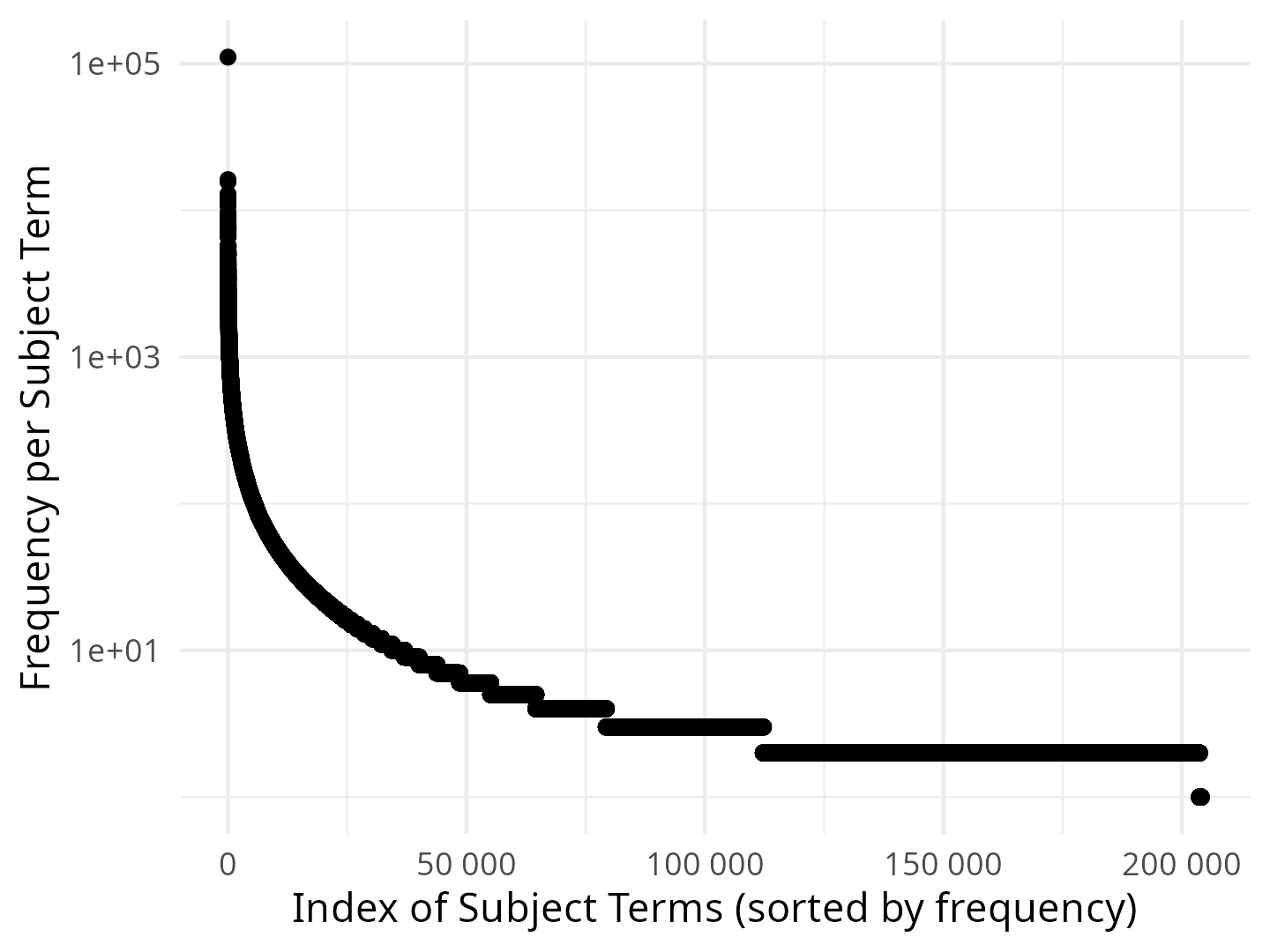
These usage statistics are based on manual subject assignments conducted by subject experts of the DNB. The process of manual subject assignment follows the German rules for subject cataloguing (RSWK1), and subject experts are trained in these rules and possess in-depth subject knowledge in their respective scientific domain.
Given the large, sparsely annotated, and highly imbalanced label set, the task of automated subject indexing can be understood as an extreme multi-label classification problem [2], [3]. Two examples of manually indexed book titles can be found in table ¿tbl:tab:example-books? in the appendix.
1.1 Related Work↩︎
XMLC problems arise in a variety of applications: [4], [5] apply the paradigm to dynamic search advertising. In [6], [7], XMLC methods are developed for item-to-item recommendation, and [8], [9] study the application to legal document classification. Benchmark datasets for these applications are collected in the Extreme Classification Repository [2]. [10], [11] put together a survey of XMLC methods. Recently, [12] contributed a public benchmark dataset containing multilingual library records also tagged with the GND. In this benchmark, the top-performing team [13], [14] has applied a combination of XMLC methods and lexical matching, using the Annif framework [15]. The same kind of ensemble modelling is applied by productive services at the DNB [16], too.
1.2 Contributions of this Work↩︎
This study is the first benchmark of XMLC algorithms on a purely German language dataset. Furthermore, we apply algorithms not only to short texts but also to longer texts, challenging their ability for long-context retrieval. In addition, the evaluation is not only based on a binary relevance comparison with previously indexed gold standard material, but also includes a graded relevance rating conducted by subject experts on previously unseen material. Finally, the benchmark of XMLC methods is complemented by the evaluation of traditional lexical matching approaches as well as newly developed embedding-based matching techniques and LLM-based few-shot prompting.
2 Datasets↩︎
2.1 Subject Vocabulary↩︎
Our datasets restrict the subject indexing tasks to a subset of the Integrated Authority File GND-204K, comprising 204 056 distinct entities. This collection includes six entity types: Subject headings, geographic names, person names,
works, conferences, and corporate entities. Table 1 summarises the numbers of distinct entities in each entity type. In the following, as a wording of convenience, we define subject term to mean any distinct entity
or concept from any of the entity groups, although this may not strictly refer to the entity group of subject headings alone, but also includes the other entity groups. For brevity, we also use the term label synonymously with the notion
of subject term. Furthermore, we refer to GND-204K as our label space or target vocabulary.
| GND Entity Type | Frequency |
|---|---|
| Geographic Names | 24 359 |
| Corporate Entities | 22 806 |
| Person Names | 44 998 |
| Subject Headings | 94 362 |
| Conferences | 1 249 |
| Works | 16 282 |
The GND-204K subset is the collection of all entities that have been used at least once in the available records of manually indexed contemporary German scientific literature in our catalogue. The GND-204K subset was created
before splitting the available gold standard records into training, development, and test sets (see the following sections).2 Therefore, each of the splits contains a portion
of rare labels, not occurring in the other splits. Labels occurring in the test set, but not in the training set, are referred to as zero shot labels.
2.2 Training dataset↩︎
We evaluate all algorithms on two tasks:
- Book-Titles
-
Subject indexing based on a document’s mere title.
- Fulltext-30k
-
Subject indexing based on the first 30 000 characters of a document’s full text.
All documents are textbooks of German scientific literature.
For each task there is a respective training and test set. Table 2 shows some descriptive statistics of the respective training datasets for each task. For development and hyper-parameter optimisation we used
additional splits dev-train and dev-test for each task. Appendix 9.2 provides further details on our four-way-hold-out strategy. Details on how the test set was used for graded relevance
evaluation are explained in the following section 2.3.
| Task | Number of Documents | Distinct Labels | \(\diameter\)Labels per Record | \(\diameter\)Records per Label | Bag-of-Words Feature Size |
|---|---|---|---|---|---|
| Training set | |||||
| Book-Titles | 951 104 | 193 921 | 2.76 | 13.5 | 650 692 |
| Fulltext-30k | 167 281 | 67 757 | 3.37 | 8.32 | 1 612 482 |
| Test set | |||||
| Book-Titles | 4 651 | 8 978 | 4.04 | 2.09 | 650 692 |
| Fulltext-30k | 4 651 | 8 978 | 4.04 | 2.09 | 1 612 482 |
Appendix 9.3 illustrates the distribution of text length for the two tasks. In particular, figure 2 (b) illustrates the length cut off at 30,000 characters. We note, that the cut off at 30,000 characters constitutes a severe restriction in terms of contents used in contrast to full length text books. However, ablation studies conducted with the Omikuji model (cf. section 3.1.2) in our productive services have indicated only a moderate loss of performance in terms of F1-Score. We hypothesise that the first 30,000 usually contain tables of contents or other summarizing parts of a book, that cover the books’ wider content. Dealing with full length text books has been computationally out of scope for this study.
2.3 Evaluation dataset↩︎
Evaluation is conducted on a shared test set for both tasks3, consisting of 4 651 documents equally distributed across 20 scientific subject groups. This ensures that all these subject categories contribute with equal weight to the evaluation, even if the training data is unevenly distributed over subject categories.4 A graded relevance evaluation by subject experts was conducted on subsamples of the test set. Note, in particular, that the graded relevance evaluation is conducted on distinct, non-overlapping, subsets of the test set so that each method was rated on 500-600 documents, respectively. This is to ensure that each record is only seen once by every subject expert. Appendix 9.1 describes the details of our sampling plan for graded relevance evaluation.
3 Methods↩︎
Given the large variety of research prototypes for extreme multi-label classification, this benchmark study selects only representatives of larger families of algorithms. The selection was based on performance in the Extreme Classification Repository Wiki500 benchmark [2] and popularity in literature at the time, as measured by google scholar citations. To have a baseline to our current library system, we included a lexical indexing method. Finally, addressing the rising prevalence of embedding-based methods and generative language models, we contrast the supervised XMLC methods with three of our own recent prototypes. Table 3 summarises some important characteristics of the algorithms included in this benchmark.
| Method | Text Representation | Supervised Approach (y/n) | Zero-Shot Capabilities (y/n) | Usage of Label Features (y/n) |
|---|---|---|---|---|
| Supervised XMLC Methods | ||||
| DiSMEC++ | sparse (Bag-of-Words, TF-IDF) | ✔ | ||
| Omikuji | sparse (Bag-of-Words, TF-IDF) | ✔ | ||
| ZestXML | sparse (Bag-of-Words, TF-IDF) | ✔ | ✔ | ✔ |
| AttentionXML | dense (Transformer + LSTM) | ✔ | ||
| XR-Transformer | sparse & dense (Transformer + TF-IDF) | ✔ | ||
| NGAME | dense (Transformer) | ✔ | ✔ | |
| Unsupervised Methods | ||||
| Lexical Matching | sparse (Bag-of-words) | ✔ | ✔ | |
| EBM | dense (Transformer) | ✔ | ✔ | |
| LLM-Ensemble | dense (Transformer) | ✔ | ✔ | |
| KI-FSPrompt | dense (Transformer) | (✔) | ✔ | ✔ |
3.1 Supervised XMLC Methods↩︎
3.1.1 DiSMEC++↩︎
A common approach for multi-label tasks are 1vsAll classifiers, where a separate classifier is trained for each label. Among others, [17], [18] propose one such algorithm, DiSMEC (Distributed Sparse Machines for Extreme Multi-Label Classification), and its successor DiSMEC++. DiSMEC features a double layer of parallelisation for distributed computing, and a capacity control mechanism to cut-off model weights to ensure compact model size. In addition, DiSMEC++ further optimises the choice of initial weights, resulting in an implicit negative mining effect. DiSMEC++ is designed to work with a sparse TF-IDF feature matrix as representation of the input texts.
3.1.2 Linear Models with Label-Partitioning Techniques↩︎
While 1vsAll classifiers perform well, training and run time scale linearly with the number of labels. As such, naively employing them for problems with a large label set is often infeasible for settings where efficient performance is necessary. To cut
down on training and inference time, [4] recursively cluster labels based on their similarity. This creates a partitioned label tree (PLT),
in which inner nodes can be considered metalabels, and node classifiers decide whether to follow a child node. As negative examples for training a classifier can be efficiently selected from a node, efficient training is possible. During inference, beam
search can be employed to avoid evaluating all node classifiers.
While [4] use binary trees with balanced label clusters, [5]
propose Bonsai, where a node can have more than two children, which leads to more shallow PLT. Additionally, Bonsai does not enforce the same size between all clusters.
For our experiments, we use Omikuji5, which implements various PLT methods with linear classifiers, re-implementing works of [4], [5] and [19] in the RUST language. Similar to DiSMEC++, Omikuji operates on sparse TF-IDF feature matrices to process input documents.
3.1.3 ZestXML↩︎
Another approach working on sparse TF-IDF feature matrices is ZestXML (Generalized Zero-Shot Extreme Multi-label Learning) by [20]. In addition to learning correlations between TF-IDF-text features and the document-label matrix, as done by all of the above-mentioned XMLC methods, this algorithm also represents labels through their TF-IDF features and correlates text features with label features directly. Another interesting feature is the ability to incorporate a label hierarchy in the label features and add this to the learnable features. As such, ZestXML has the ability to also infer on Zero-Shot labels, if some of their label features have been seen in the training material.
3.1.4 AttentionXML↩︎
Earlier approaches for XMLC usually rely on bag-of-words representations of input documents, like TF-IDF matrices. AttentionXML by [19] employs
an LSTM, a recurrent deep-learning architecture, for XMLC, which is able to capture more context-dependent relations within an input document. Additionally, a label-wise attention mechanism is employed, which allows for separate input representation for
each label. [19] also cluster labels in a PLT for efficient training and inference, but in contrast to approaches like [4] and [5], AttentionXML trains classifiers in a layer-wise fashion, where neural
networks in deeper layers of the PLT are initialised with parameters of the previous layer for fast convergence. Like [5], the authors opt for a more shallow
label tree, which is achieved via layer collapsing.
In our experiments, we found initial performance to be low due to a high number of unknown tokens when using the originally proposed fasttext word tokenisation. Instead, we use Byte-Pair Encoding tokenisation, which splits unknown words into
previously encountered subwords. We then initialise (sub-)word embeddings from a BERT embedding layer.
3.1.5 XR-Transformer↩︎
The Transformer architecture with a self-attention mechanism has been long established as state-of-the-art for many natural language processing tasks [21]. Transformer models like BERT [22] are usually pre-trained in an unsupervised manner on large text corpora before they are fine-tuned on task-specific datasets. [6], [7] adapt transformers for extreme multi-label classification. Similar to previously discussed approaches, a label tree is employed. A pre-trained encoder model is fine-tuned layer-wise on the meta-label classification tasks. For the final predictions, linear classifiers are trained on the concatenation of the fine-tuned, dense Transformer embeddings and the sparse TF-IDF vectors.
3.1.6 NGAME↩︎
Many approaches for XMLC, like by [19] and [7], treat labels as mere identifiers. However, labels are often associated with textual data. As such, this side-information can be leveraged for extreme multi-label classification, as also attempted by [20]. NGAME [23] makes use of textual data associated with labels by embedding both input documents and label texts with a pre-trained encoder model, and minimizing the distance between the embeddings of input documents and their associated labels. A challenge for this set-up is the selection of informative hard negative examples to train on: [23] employ curriculum learning, where batches are constructed based on clusters with similar embeddings. Negative examples can be efficiently sampled from the same batch. As the cluster size decreases during training, examples in a batch become more similar, and as such more difficult negative labels are introduced.
3.2 Unsupervised Approaches↩︎
3.2.1 Lexical Matching↩︎
Subject indexing can also be approached as an instance of keyphrase extraction [24]. A special case is keyphrase extraction using lexical matching [25]. In [26], [27], the algorithm Maui was introduced. Maui combines the lexical matching with a candidate ranking, based on heuristics acquired during the lexical matching process: How often does the match occur in a text? What was its position in the text? What is its distribution throughout the document? These heuristics are used to train a small ranker model with a much smaller training dataset than in the above-mentioned supervised XMLC methods.6 The Annif toolkit also implements the idea of lexical matching in its backend MLLM (Maui Like Lexical Matching) [28], which we include as a baseline in our benchmark.
3.2.2 Embedding Based Matching (EBM)↩︎
The idea of lexical matching can be “modernised” by relying on embedding-based matching instead of lexical matching. This is closely related to the idea of dense retrieval models [29]. Both input documents and vocabulary can be vectorised by using a pre-trained sentence encoder model, e.g., BGE-m3 [30] or jina-embeddings-v3 [31]. Vector search across the vocabulary creates candidate matches. As in Maui or
MLLM, these candidate matches can be reranked using a small ranking model trained on similar heuristics that are captured during the matching process (frequency of occurrence, position, spread). This idea is implemented in the ebm4subjects
package [32].
3.3 Methods using generative LLMs↩︎
3.3.1 LLM-Ensemble↩︎
The LLM-Ensemble [33] approaches the subject indexing problem by combining multiple LLMs with multiple fixed few-shot prompts. The LLM-generated
subject terms are mapped to the vocabulary via hybrid search, and further post-processing steps combine the individual suggestions to an ensemble vote. This approach only needs a small number of examples filling the few-shot prompts, so there is no need
for training. However, calling multiple LLMs with multiple prompts per document comes with high inference costs. In particular, longer texts that are processed chunkwise require many LLM-calls at inference time. Language models included in the LLM-Ensemble
for completing few-shot prompts are Llama-3B-Instruct, Llama-70B-Instruct, Mistral-7B-v0.1, Mistral-7B-Instruct-v0.3, Mixtral-8x7BInstruct-v0.1, OpenHermes-Mistral-7B, and
Teuken-7B-instruct-research-v0.4. In addition, Llama-8B-Instruct is used as ranking model.
3.3.2 KI-FSPrompt↩︎
KI-FSPrompt [34] is another system that leverages the idea of few-shot prompting, to generate subject terms with a generative LLM. As an attempt to
mitigate the high inference costs of the LLM-Ensemble, the system KI-FSPrompt alters the approach of the LLM-Ensemble by replacing the fixed few-shot prompts with a per-document RAG-like retrieval step, where few-shot prompts are assembled dynamically with
examples from the training dataset that are close to the requested document (in terms of embedding similarity). We use KI-FSPrompt with Mistral-7B-Instruct-v0.3 and Llama-3.2-3B-Instruct as models for prompt-completion, and
Meta-Llama-3.1-8B-Instruct as a ranking model.
4 Metrics↩︎
In this benchmark study, we use binary relevance and graded relevance metrics.
4.1 Binary Relevance↩︎
For binary relevance, we compare the machine-based subject suggestions with the gold standard, annotated by subject experts according to the German rules for subject cataloguing (RSWK). All algorithms studied in this benchmark produce a list of subject
suggestions, where every subject suggestion comes with some confidence score that can be used to obtain a ranked list of subject suggestions per document. Therefore, standard metrics for ranked retrieval apply. However, in practice, one would usually
filter predictions with some uniform limit \(k\) on ranks and threshold \(t\) on confidence scores to filter out the most relevant suggestions for a productive system. Focus on high recall
or high precision depends on the use case: an unsupervised cataloguing system needs to be calibrated more strictly to achieve high precision; in a supervised (assisted) workflow, producing high recall is more important. To measure the performance over the
entire ranking, we look at precision-recall curves: for any given limit \(k\) and threshold \(t\), we compute the document average (doc-avg) precision and recall. For every level of recall,
there is an optimal configuration of limit and threshold achieving highest precision. This defines the precision-recall curve (\(\mathcal{C}_\mathrm{pr}\)). Computing the integral of the pr curve gives rise to the measure
of the Area under the Precision-Recall Curve (\(\mathrm{AUC}_{\mathrm{pr}}\)). \(\mathrm{AUC}_{\mathrm{pr}}\) will be our primary measure for algorithmic performance. To
give some point estimates of a system’s performance, we also compare their optimal (document average) \(F^1\)-score, denoted as \(F^{1,*}\), that could be attained by applying an optimal
calibration of limit and threshold to the system. See appendix 12.2 for details on how we avoid in-sample bias in this estimation and see appendix 12 for full
definitions of all metrics. These can be computed using our public R package CASIMiR7.
4.2 Binary Relevance with Conditional Weighting↩︎
In the evaluation of subject indexing methods, it is very important to also take performance on long-tail labels into consideration. Otherwise, algorithms that simply ignore rare labels and focus on head labels will dominate rankings. However, in large controlled subject vocabularies, the nuanced, most specialised topics are those of highest interest for users in search of specific literature. To study the performance in the long-tail of our vocabulary, we introduce weighted variants of the above metrics that use a specific cost scheme. True positives (\(\text{tp}\)) and false negatives (\(\text{fn}\)) are weighted by a label-dependent cost factor that is based on inverse propensity scores [3]. We denote these conditionally propensity scored metrics as \(\mathrm{cps-Rec}, \mathrm{cps-Prec}, \mathrm{cps-F}^1\) and \(\mathrm{cps-AUC}_\mathrm{pr}\), and report them separately. See appendix 12 for details.
4.2.1 Graded Relevance↩︎
Whereas binary relevance comparison treats all false positive suggestions as simply wrong, the graded relevance rating allows comparing to what degree false positive suggestions still constitute helpful subject assignments, even if they would not be assigned after RSWK rules. In the graded relevance scenario, subject experts directly rate the top 5 machine-based subject suggestions for each algorithm and task. They use an ordinal scale of (0) false, (1) slightly useful, (2) useful and (3) very useful. Here, usefulness is defined by a subject term’s suitability as a search query to find a particular document in the catalogue. This is a notion of usefulness that takes the user’s perspective into account, as opposed to strict adherence to the German rules for subject cataloguing, which is measured by the binary relevance comparison with the gold standard. To compare the algorithms in this graded relevance scenario, we use the metrics generalised precision \(\mathrm{g-Prec}\) and generalised recall \(\mathrm{g-Rec}\) as defined in [35]. See appendix 12.4 for further details.
5 Results↩︎
5.1 Binary Relevance Results↩︎
| Book-Titles | Fulltext-30k | |||||||
|---|---|---|---|---|---|---|---|---|
| 2-5 (lr)6-9 Method | \(F^{1,*}\) | \(\textup{AUC}_\textup{pr}\) | \(\textup{cps-}F^{1,*}\) | \(\textup{cps-AUC}_\textup{pr}\) | \(F^{1,*}\) | \(\textup{AUC}_\textup{pr}\) | \(\textup{cps-}F^{1,*}\) | \(\textup{cps-AUC}_\textup{pr}\) |
| DiSMEC++ | 0.426 | 0.402 | 0.386 | 0.368 | 0.361 | 0.354 | 0.305 | 0.306 |
| Omikuji | 0.417 | 0.395 | 0.370 | 0.354 | 0.343 | 0.329 | 0.277 | 0.273 |
| AttentionXML | 0.367 | 0.342 | 0.298 | 0.282 | 0.188 | 0.124 | 0.124 | 0.083 |
| XR-Transformer | 0.467 | 0.427 | 0.421 | 0.389 | 0.398 | 0.359 | 0.339 | 0.307 |
| NGAME | 0.391 | 0.366 | 0.383 | 0.369 | NA | NA | NA | NA |
| ZestXML | 0.379 | 0.369 | 0.359 | 0.356 | 0.336 | 0.295 | 0.301 | 0.267 |
| KI-FSPrompt | 0.453 | 0.340 | 0.436 | 0.339 | NA | NA | NA | NA |
| LLM-Ensemble | 0.382 | 0.308 | 0.379 | 0.316 | 0.364 | 0.333 | 0.362 | 0.345 |
| Emb.-based matching | 0.285 | 0.212 | 0.274 | 0.214 | 0.309 | 0.279 | 0.295 | 0.274 |
| Lexical Matching (MLLM) | 0.274 | 0.148 | 0.266 | 0.146 | 0.303 | 0.268 | 0.277 | 0.253 |
Table 4 shows the results of the binary relevance comparison for both tasks. The ranking of methods in terms of \(\mathrm{AUC}_{\mathrm{pr}}\) and optimal \(F_1\)-score \(F^{1,*}\) is not consistent between the two metrics. Notably, the supervised XMLC methods, XR-Transformer, Omikuji, and DiSMEC++, lead the ranking for both tasks in terms of \(\mathrm{AUC}_{\mathrm{pr}}\). Interestingly, while XR-Transformer outperforms the other methods by a significant margin for the Book-Titles task, the difference between DiSMEC++ and XR-Transformer is hardly notable
for Fulltext-30k. We hypothesise that, due to the relatively short context length of the finetuned transformer, little is to be gained from the transformer part here, and most predictive power is coming from the TF-IDF features alone. The
AttentionXML algorithm, not relying on bag-of-words features at all, shows complete failure in the Fulltext-30k task: only little information can be gained from looking at the very small context window allowed by AttentionXML when looking at a
full text.8 The title alone is more informative for AttentionXML’s LSTM architecture. While most methods achieve higher results in the Book-Titles task, we see
the opposite for the ontology-based matching methods, MLLM and EBM. Both methods benefit from processing more text material. Neither in the Book-Titles task nor in the Fulltext-30k task do the supervised methods that make use of
the label features (NGAME, ZestXML) show distinguished results.
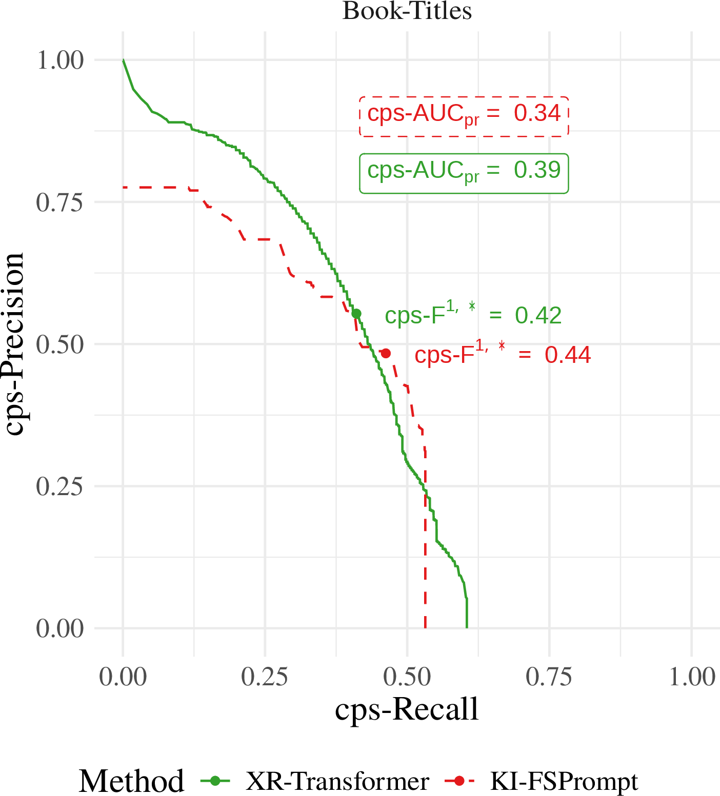
Looking at the conditionally propensity scored metrics in table 4, emphasising the long-tail performance of the methods, we see a slightly different ranking. The LLM-based KI-FSPrompt is ahead of XR-Transformer for the
Book-Titles task in the point estimate of \(\mathrm{cps-}F^{1,*}\), but not \(\mathrm{cps-AUC}_{\mathrm{pr}}\). The precision-recall curve in figure 3 in the appendix 11 illustrates the situation. In the Fulltext-30k task, the LLM-Ensemble is clearly on top of the other methods, followed by XR-Transformer and DiSMEC++.
In these weighted metrics, even the lexical matching and embedding-based matching can best the supervised partitioned label tree approach, Omikuji. We illustrate these findings in appendix 11.2, showing estimates
of the subject average \(F^1\)-score by label frequency.
5.2 Graded Relevance Results↩︎
@>
mm>
m>m>
m>m>
m>m>
m>m>
m>m>
m>m
& & &
(lr)2-7 (lr)8-13 Method & \(\textup{g-}F^{1}_5\) & 95% CI & \(\textup{g-Prec}_5\) & 95% CI & \(\textup{g-Rec}_5\) & 95% CI & \(\textup{g-}F^{1}_5\) & 95% CI & \(\textup{g-Prec}_5\) & 95% CI &
\(\textup{g-Rec}_5\) & 95% CI & \(N_{\textup{docs}}\)
AttentionXML & & [0.514, 0.536] & 0.533 & [0.526, 0.547] & 0.565 & [0.553, 0.584] & 0.337 & [0.331, 0.353] & 0.344 & [0.337, 0.361] & 0.361 &
[0.354, 0.375] & 524
Emb.-based matching & 0.433 & [0.420, 0.443] & 0.440 & [0.425, 0.449] & 0.473 & [0.463, 0.487] & 0.488 & [0.481, 0.497] & 0.498 & [0.489, 0.505] &
0.527 & [0.520, 0.543] & 528
LLM-Ensemble & 0.576 & [0.570, 0.583] & 0.604 & [0.597, 0.610] & 0.593 & [0.586, 0.607] &
0.601 & [0.595, 0.601] & 0.634 & [0.627, 0.638] & 0.611 & [0.597, 0.615] & 555
Omikuji & 0.499 & [0.492, 0.521] & 0.516 & [0.512, 0.537] & 0.531 & [0.518, 0.560] & 0.525 & [0.513, 0.531] & 0.561 & [0.550, 0.566] & 0.537 &
[0.525, 0.547] & 534
XR-Transformer & 0.530 & [0.520, 0.545] & 0.537 & [0.529, 0.552] & 0.581 & [0.567, 0.595] & 0.512 & [0.502, 0.521] & 0.531 & [0.521, 0.540] & 0.543
& [0.533, 0.550] & 586
ZestXML & 0.459 & [0.454, 0.470] & 0.454 & [0.449, 0.463] & 0.522 & [0.518, 0.538] & 0.451 & [0.440, 0.456] & 0.448 & [0.437, 0.457] & 0.508 &
[0.493, 0.513] & 542
Table ¿tbl:tab:graded95rel? shows the results of the graded relevance ratings in terms of generalised precision, recall, and \(F_1\)-score at limit \(k=5\). We observe
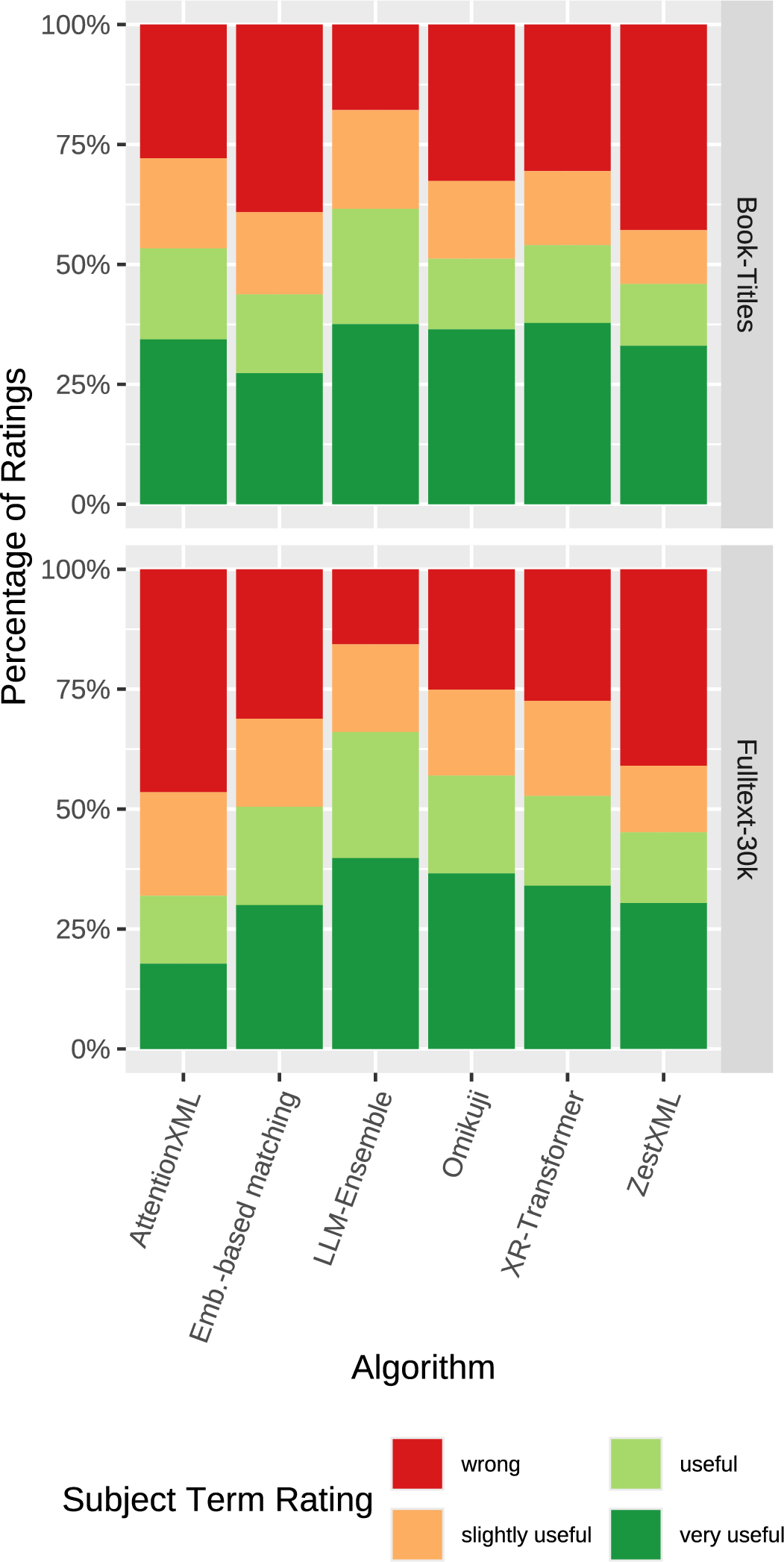
that the LLM-Ensemble method is ahead of all other methods in both tasks. Figure 5 in appendix 11 offers some explanation: While the portion of subject-term predictions rated as "very
useful" is only marginally larger than those generated by other methods, there is a much larger portion of "useful" and "slightly useful", so that the LLM-Ensemble does not produce as many "wrong" predictions as the other methods. Another takeaway is that
in the Book-Titles task, the supervised XMLC methods with dense feature representations (Transformer/LSTM), namely XR-Transformer and AttentionXML, score higher than the TF-IDF-based Omikuji and ZestXML. This is not the case in the
Fulltext-30k task. In terms of generalised recall, the EBM method almost reaches the performance of supervised methods for the Fulltext-30k task, which would qualify EBM as a suitable method for assisted subject indexing workflows
with little training material.
5.3 Inference Time↩︎
Due to the complexity of the benchmarking process and changing hardware setups during the course of the project, this project did not maintain comparable records of training and inference times for all algorithms in both tasks. Nevertheless, this is a
vital component of evaluation. We therefore include a comparison of inference times for the Book-Titles task computed on a 2 x Intel(R) Xeon(R) Gold 6338T CPU @ 2.10GHz (48 core) architecture with two NVIDIA A100 80GB GPU processors.
Table ¿tbl:tab:inference-time? displays the inference times.
| Method | Inference Time p. rec. in ms |
|---|---|
| DiSMEC++ | <1 |
| Omikuji | <1 |
| AttentionXML | 3 |
| XR-Transformer | 10.5 |
| NGAME | 1.6 |
| ZestXML | <1 |
| KI-FSPrompt | 271 |
| LLM-Ensemble | 998 |
| Emb.-based matching | 9.4 |
| Lexical Matching (MLLM) | 23 |
40 parallel CPU-processes
1 NVIDIA A100 GPU
Setup requires 2 NVIDIA A100 GPU
We observe that LLM-based methods are more resource-intensive by at least two orders of magnitude, compared to the other methods. In particular, the LLM-Ensemble, requiring several calls per record to larger 56B to 70B models, does not only raise the
demand for appropriate hardware (two GPUs required), but reaches processing times that must be judged as infeasible for processing large amounts of data in daily library processes. While for practical reasons we do not include a similar table for the
Fulltext-30k, the inference times in this case are, of course, much higher for all methods. Particularly, LLM-Ensemble, Emb.-based matching and Lexical Matching (MLLM) scale linearly with text length. For Emb.-based matching the generation of
embeddings for longer texts can become a severe bottleneck.
6 Limitations↩︎
This benchmark focuses on scientific literature as indexed by the German National Library, and therefore may not generalise to other domains or document types (e.g., grey literature, newspapers, or popular science) or other languages. The GND, while comprehensive, is tailored to specific cultural and scholarly needs in German-speaking contexts and contains idiosyncrasies that may affect transferability to other more specialised authority files or ontologies. One particular point to note is, that this study makes the simplifying assumption to treat all entity types of the GND as the same. Arguably, named entities are linguistically different from subject headings, when it comes to their assignment as relevant labels to a text. The attribution to a text for named entities is usually a binary decision, whereas subject headings may have varying degrees of relevance for a particular text. This is not addressed within the XMLC-setting of this study.
Moreover, we were only able to compare a limited number of algorithms. During the elapse of our project, new algorithms, such as Renee [36] or ViXML [37], were released, offering potential advancement on the state-of-the-art. The authors regret that these could not be investigated to full extent. Not only the selection of algorithms but also the time spent adapting the algorithms for our data, with hyper-parameter optimisation, is subjective. One-Vs-All-Classifiers are considerably easier to parametrise as opposed to transformer-based methods, which open up an almost uncontrollable degree of potentially relevant hyperparameters9. The authors have experimented with these hyperparameters to the best of their knowledge, fully aware that poor performance may always occur, which can be attributed to a combination of the inability to control the investigated program and the inadequacy of the proposed algorithm.
Another class of hyperparameters influencing the study is related to the preprocessing of the texts. One such parameter is the selection, which parts of a fulltext book should be processed, if not all. [16] have experimented with Table-of-Contents (TOC) as a high quality source of training material. Future work should investigate this as an intermediate level of
information complexity between the Book-Titles and Fulltext-30k tasks. Given the length of the academic textbooks in our collection, as illustrated in appendix 9.3, dealing with full length
text books has been computationally out of scope for this study.
Other preprocessing parameters concern the vectorisation and tokenisation for the TFIDF text representations. While these parameters may seem less dramatic, in contrast to text length, they do have direct impact on feature size and, thus, computational complexity for the more traditional approaches. While initial ablation studies where conducted, the impact of the vectorisation was not studied in detail for all methods.
Further limitations of this study concern the graded relevance ratings. The resources of our subject experts for graded relevance ratings are limited. We could not afford having all algorithms rated by the experts, so we restricted this part to those methods most promising during preliminary investigations that were suitable to be evaluated on both tasks. These time and resource constraints sadly excluded our final prototype KI-FSPrompt, which would have been interesting to evaluate in the graded relevance setting, too.
Another note of warning relates to the LLM-based approaches: it is impossible to capture the state-of-the-art in LLM-based approaches, due to the rapid advancements of methods and models in recent years. The LLM-Ensemble and KI-FSPrompt used in this study are just snapshots in an evolving landscape. Benchmarking LLM-based approaches would legitimise a new benchmark study on its own.
An aspect that should have taken a prominent place in this study is the evaluation of training and inference times. However, in the course of our project, we have changed and switched hardware environments (between local and HPC-based deployment) multiple times, which makes a consistent comparison rather difficult.
Finally, there is a gap to bridge between the prototypes resulting from this research and the requirements in the productive library process of automated indexing. We recommend for library practitioners to construct their productive systems around Annif, ultimately working toward increasing the availability of new backends in the Annif ecosystem.
7 Conclusion and Future Work↩︎
This study has contributed to the understanding of weaknesses and strengths of the various algorithmic approaches to automated subject indexing. We see that supervised and matching-based approaches, even in the age of generative LLMs, still have their benefits and strengths. In terms of absolute metrics, the supervised XMLC approach XR-Transformer shows best results. In terms of vocabulary coverage and performance for less frequent labels, the LLM-based approaches deliver higher quality, as confirmed by our graded expert ratings.
Future work should be directed towards refining the KI-FSPrompt pipeline, which seems to be the most promising among our prototypes. In particular, more research is needed on developing approaches that can also efficiently handle the content of longer documents, which cannot easily be processed as few-shot examples in a single prompt.
Finally, this study has focused on evaluating single backend algorithms. In practice, productive systems should combine the most promising methods into ensemble methods to achieve the best performance. Here, further research is needed to identify component models for such ensembles, as well as methods for ensembling that can successfully manage the challenges posed by large label spaces.
8 Acknowledgements↩︎
This work is a result of a research project at the German National Library (DNB)10. The project was funded by the German Minister of State for Culture and the Media as part of the national AI strategy. We extend our thanks to all of our subject librarians, whose countless hours of dedicated effort made the graded relevance ratings possible. Furthermore, the authors gratefully acknowledge the computing time made available to them on the high-performance computer at the NHR Center of TU Dresden. This center is jointly supported by the Federal Ministry of Research, Technology and Space of Germany and the state governments participating in the NHR11. Finally, we thank the anonymous reviewers for their kind and helpful feedback.
9 Datasets↩︎
9.1 Sampling plan for graded relevance ratings↩︎
The test set above consists of six data slices, each having the same distribution of main DDC Subject Categories as the whole test set. To ensure that the publications were not seen before, each algorithm was tested on a distinct data slice. Due to resource considerations, in the graded relevance scenario, not all methods could be rated by subject experts. So only a subset of six methods could be included. Also, only top 5 predictions per algorithm and task could be rated.
The test set was clear of gold standard annotations before the beginning of the evaluation phase. Over a course of three years, subject experts successively rated machine-based suggestions for one algorithm per slice.12 Afterwards they were asked to complete the metadata record according to the rules of RSWK, also filling in missing aspects not discovered by the algorithms. The resulting test set has full gold standard annotations for all 4 651 documents and graded relevance ratings for one slice per method. Therefore, graded relevance metrics are based on distinct data slices per method, whereas results for binary relevance metrics all rely on the full test set.
9.2 Additional Statistics on Datasets↩︎
To avoid optimisation bias in the training and hyper-optimisation, we worked according to a four-way-hold-out strategy: In addition to the training set and test set described in section 2, we chose two validation sets,
dev-train and dev-test, for each task. The dev-train splits were sampled from the same distribution as the training data with a stratified sampling technique by [38], separately for each task. This ensures that the dev-train splits holds as many as possible of the labels also seen during training and is therefore similar in composition to the
training set. For dev-test, however, the data is sampled in equal bins of the same scientific main subject categories also represented in the test set. This ensures that all main subject categories contribute with equal weight to the
evaluation, even if the training data is unevenly distributed over main subject categories. The purpose of dev-train is to control learning and overfitting during training. The purpose of dev-test is for hyper-parameter
optimisation, including threshold and limits to determine optimal precision-recall balance as in section 12.2. The documents contained in the dev-test split are the same for both tasks,
allowing direct comparison between the tasks. Table 5 shows further descriptive statistics on the development sets.
| Task | Training | Dev-Train | Dev-Test |
|---|---|---|---|
| Number of Documents | |||
| Book-Titles | 951 104 | 73 320 | 8 415 |
| Fulltext-30k | 167 281 | 24 315 | 8 415 |
| Number of Labels | |||
| Book-Titles | 193 921 | 97 894 | 11 387 |
| Fulltext-30k | 67 757 | 40 703 | 11 387 |
9.3 Length Distribution of Training Data↩︎
This appendix provides information on the length distribution of training texts for the respective tasks. Table 6 shows distributional statistics for Book-Titles, Fulltext and
Fulltext-30k. Here, Fulltext refers to the full length text books without cut off, whereas Fulltext-30k applies a uniform cutoff.
| Task | Min | Q1 | Median | Mean | Q3 | Max |
|---|---|---|---|---|---|---|
| Book-Titles | 1 | 40 | 65 | 75 | 97 | 1 472 |
| Fulltext | 123 | 291 055 | 504 671 | 632 410 | 812 156 | 10 129 426 |
| Fulltext-30k | 123 | 29 993 | 29 997 | 29 565 | 29 999 | 30 000 |
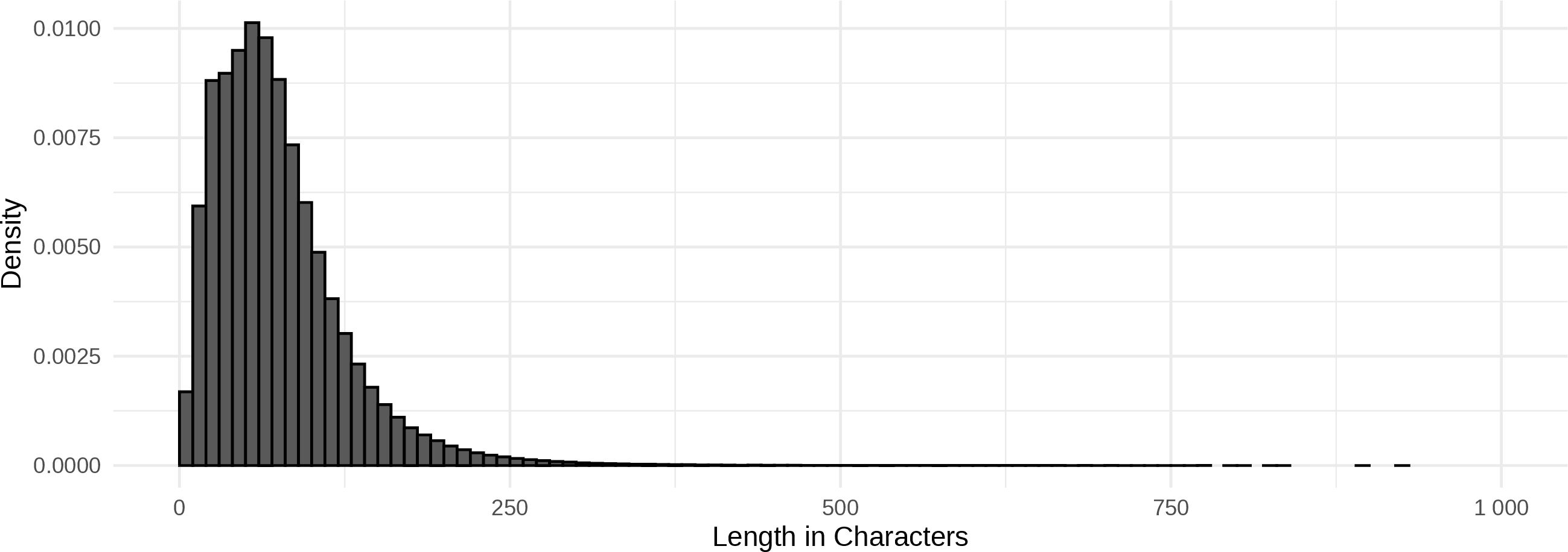
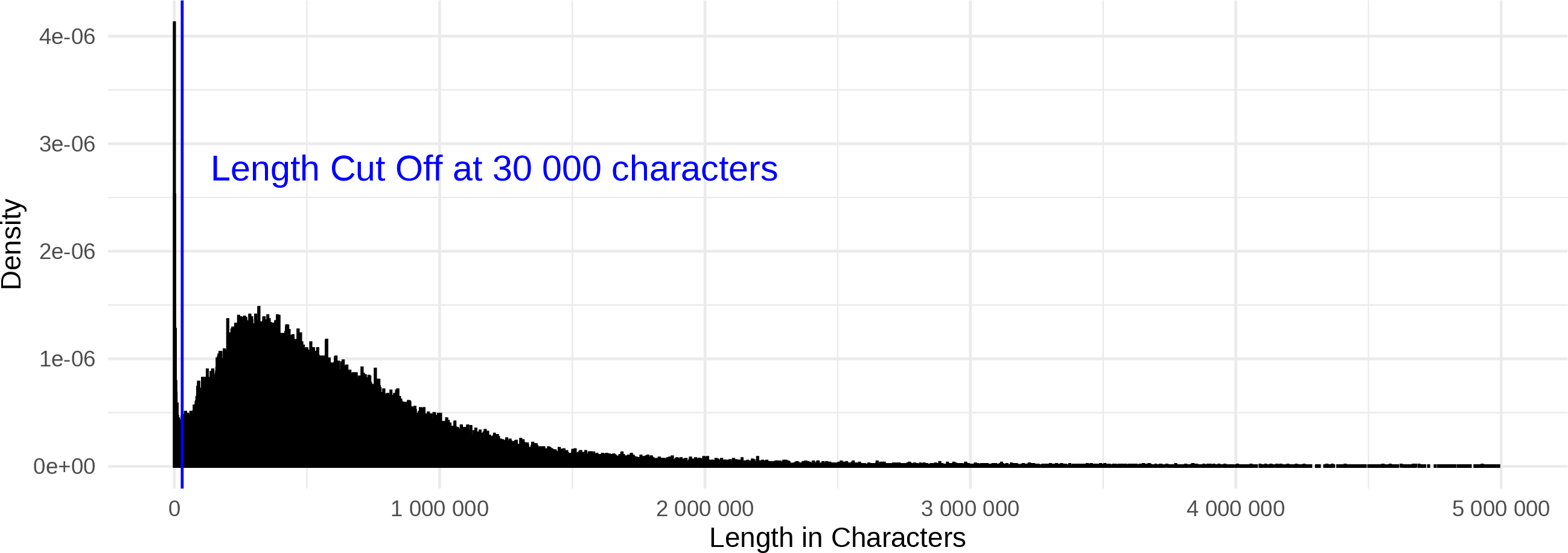
Figure 2: Distribution of training text length for tasks Fulltext and Book-Titles.. a — Task Book-Titles, b — Task Fulltext
10 Examples↩︎
Table ¿tbl:tab:example-books? shows two examples from our catalogue along with their respective subject terms according to RSWK. In practice, subject librarians have access to the full document text, so it is not always possible to
infer all gold standard subject terms from a book title alone. Therefore, in the Book-Titles task, we must expect that there is a certain amount of infeasible subject terms that can never be found by any of the methods.
p0.43
11 Additional Results↩︎
In this appendix section we provide additional data analysis to give a better understanding of the results presented in the main results section 5.
11.1 Precision-Recall Analysis↩︎
Figure 3 highlights that, while KI-FSPrompt achieves the highest point estimate for \(\mathrm{cps}-F^{1,*}\), XR-Transformer maintains a higher \(\mathrm{cps-AUC}_{\text{pr}}\). KI-FSPrompt only produces short lists of subject suggestions per record, varying in length between 3-10 subject terms. XR-Transformer obtains confidence scores for all labels, enabling arbitrary length of subject suggestion lists.
11.2 Performance by label frequency↩︎
The following additional analysis compares the subject average performance for selected methods as a function of label frequency in the training dataset. For any given label in GND-204K we compute the \(F^1\)-score in analogy to eq. (6 ). From these label-wise scores we estimate a continuous spline with the R package mgcv [39] as a function of training frequency. To illustrate how many data points support any region of the spline, we include the marginal histogram that plots the distribution of labels in the test set. Figure 4 (a) shows the results for task Book-Titles and figure 4 (b) for task Fulltext-30k. Note that the marginal distribution differs between the two tasks,
even though both tasks share the same test set. The training dataset for task Book-Titles is much larger than for task Fulltext-30k. Hence, labels that appear as few- or zero-shot for Fulltext-30k move further to the
range of common labels in Book-Titles.
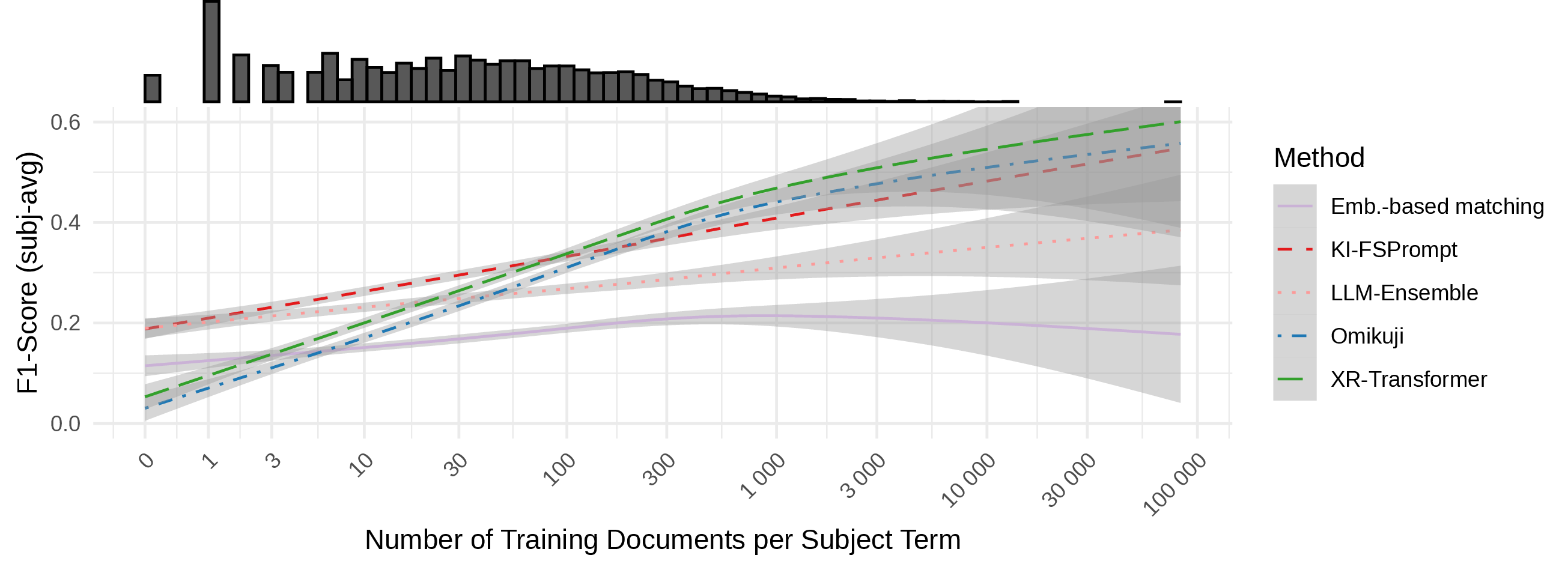

Figure 4: Subject-average \(F^1\)-Score plotted as a function of label frequency.. a — Task Book-Titles, b — Task Fulltext-30k
A key takeaway from this analysis is that the LLM-based methods provide a wider coverage of the vocabulary, whereas supervised XMLC methods excel mainly in the domain of frequent labels. LLM-Ensemble and EBM are not trained, so the quality does not increase notably for more frequent labels. However, KI-FSPrompt, leveraging the training dataset to collect similar documents as few-shot examples, shows a similar increase in quality with training frequency as the supervised models.
11.3 Graded Relevance Ratings↩︎
Figure 5 shows the relative distribution of graded relevance ratings as conducted by our subject experts.
12 Full metric definitions↩︎
This benchmark study uses some non-standard metric definitions. To make the precise calculations transparent, we include the full definitions of all metrics in this appendix.
12.1 Binary Relevance Scenario↩︎
Let \(\boldsymbol{y}_d = \{y_{d,l}\}_{l=1}^L \in \{0,1\}^L\) be the binary indicator for gold standard subject terms of document \(d = 1, \ldots, N_{\mathrm{test}}\) with labels \(l = 1, \ldots, L\), according to the subject experts. Here, \(L\) denotes the size of our vocabulary (i.e. the label space) and \(N_{\mathrm{test}}\) is the
number of documents in our test set. Likewise, let \(\hat{\boldsymbol{y}}_d = \{\hat{y}_{d,l}\}_{l=1}^L \in \{0,1\}^L\) denote an algorithm’s subject predictions with confidence levels \(\hat{\boldsymbol{c}}_d = \{ \hat{c}_{d,l}\}_{l=1}^L \in \left[0,1\right]^L\). Let \[\mathrm{Thres}_t (\hat{\boldsymbol{y}}_d) := \{l ~|~ \hat{c}_{d,l} >= t\}\] be the set of label
predictions above a threshold \(t\) and \[\mathrm{Top}_k (\hat{\boldsymbol{y}}_d) := \{l~|~\#\{ l'~|~\hat{c}_{d,l'} > \hat{c}_{d,l} \} < k \}\] be the top k ranked labels for
some integer \(k\). We define \(\mathrm{tp}_k\) (true positives), \(\mathrm{fp}_k\) (false positives) and \(\mathrm{fn}_k\)
(false negatives) as follows: \[\begin{align} \tag{1}
\mathop{\mathrm{\mathrm{tp}_k}}\left(\boldsymbol{y}_d, \hat{\boldsymbol{y}}_d\right) &:= \sum_{l \in \mathrm{Top}_k (\hat{\boldsymbol{y}}_d)} y_{l,d} \\ \tag{2}
\mathrm{fp}_k \left(\boldsymbol{y}_d, \hat{\boldsymbol{y}}_d\right) &:= \sum_{l \in \mathrm{Top}_k (\hat{\boldsymbol{y}}_d)} \left(1 - y_{l,d}\right) \\ \tag{3}
\mathrm{fn}_k\left(\boldsymbol{y}_d, \hat{\boldsymbol{y}}_d\right) &:= \sum_{l \notin \mathrm{Top}_k (\hat{\boldsymbol{y}}_d)} y_{l,d}
\end{align}\] and use the standard definitions for document-wise precision and recall
\[\label{eq:prec95k} \mathrm{Prec}_k\left(\boldsymbol{y}_d, \hat{\boldsymbol{y}}_d\right) := \frac{\mathrm{tp}_k}{\mathrm{tp}_k + \mathrm{fp}_k}\tag{4}\] and
\[\label{eq:rec95k} \mathrm{Rec}_k\left(\boldsymbol{y}_d, \hat{\boldsymbol{y}}_d\right) := \frac{\mathrm{tp}_k}{\mathrm{tp}_k + \mathrm{fn}_k}.\tag{5}\] Likewise, we have \(\mathrm{Prec}_{k,t}\) and \(\mathrm{Rec}_{k,t}\), where the sum is built over \(l \in \mathrm{Top}_k (\hat{\boldsymbol{y}}_d) \cap \mathrm{Thres}_t
(\hat{\boldsymbol{y}}_d)\), applying threshold and limit simultaneously. The document-wise \(F^1\)-Score is defined as13
\[\label{eq:f1-def} F^{1}_{t,k} (\boldsymbol{y}_d, \hat{\boldsymbol{y}}_d) := \frac{2 \cdot \mathrm{tp}_k}{ 2 \cdot \mathrm{tp}_k + \mathrm{fp}_k + \mathrm{fn}_k }\tag{6}\] The
document-average (doc-avg) Precision is defined as \[\mathrm{Prec}_{k,t} := \frac{1}{N_{\mathrm{docs}}} \sum_{d=1}^{N_{\mathrm{docs}}} \mathrm{Prec}_{k,t} (\boldsymbol{y}_d, \hat{\boldsymbol{y}}_d)\] and analogously for
Recall and F-score. The precision-recall curve \(\mathcal{C}_{\mathrm{pr}}\) is defined pointwise for a given level of recall \(R\) \[\mathcal{C}_{\mathrm{pr}}(R)
:= \max_{k,t} \left\{ \mathrm{Prec}_{k,t}~|~\mathrm{Rec}_{k,t} >= R \right\}\] and the area under the precision-recall curve is defined as \[\mathrm{AUC}_\mathrm{pr} := \int_0^1 \mathcal{C}_{\mathrm{pr}}(r)
\mathrm{d}r\] Note that the pr curve here is built on document-average precision and recall, and the search space is over limits \(k\) and thresholds \(t\) at any given point of the
pr curve. All metrics are calculated using our public R package CASIMiR.14
12.2 Mediating In-Sample Bias for Estimation of Optimal F-Score↩︎
To avoid in-sample bias for \(F^{1,*}\), we calculate the optimal thresholds and limits with pr curves on a separate dev-test-set which follows a similar distribution as test, i.e. has a similar
composition across subject categories. See also section 9.2.
12.3 Metrics with conditional label weights↩︎
In the above metrics, false positives (\(\mathrm{fp}\)), true positives (\(\mathrm{tp}\)) and false negatives (\(\mathrm{fn}\)) enter the formula for precision and recall using the standard formulae (4 ) and (5 ). To study the performance in the long tail of our vocabulary, we introduce a specific cost scheme:
| Gold standard y | Gold standard n | |
|---|---|---|
| prediction y | \(C_{\textup{tp}}\cdot \textup{tp}\) | \(C_{\textup{fp}}\cdot\textup{fp}\) |
| prediction n | \(C_{\textup{fn}}\cdot\textup{fn}\) | omitted |
Here \(C_{\mathrm{tp}}\), \(C_{\mathrm{fp}}\) and \(C_{\mathrm{fn}}\) are the costs for true positives, false positives and false negatives, respectively. Such cost factors can be used to introduce preferences in the evaluation metrics. Our special focus is on rare subjects: We argue that rare subjects are more informative and, thus, more costly to be missed out and hence the cost of a false negative should be inversely proportional to the number of training documents for that subject. The same holds true for true positives, i.e. it should be encouraged getting rare subjects right. However, getting rare subjects wrong is just as bad as getting a frequent subject wrong. Therefore, the cost of false positives is assumed to be the same for all subjects, independently of their frequency of occurrence. As weights we propose the inverse propensity scores according to [3]: \[C_{\mathrm{tp}} = C_{\mathrm{fn}} := w_{l} = 1 + C\cdot (n_{l} + B)^{-A},\] where \(C = (\log N_{\mathrm{train}} - 1)\cdot (B + 1)^A\), \(N_{\mathrm{train}}\) is the total number of training documents, \(n_{l}\) the frequency of occurrence of \(l\) within the train set and \(A, B\) are free parameters. [3] propose \(A = 0.55\) and \(B = 1.5\). For the false positive cost, \(C_{\mathrm{fp}}\), we chose a label independent cost calculated as the mean of all \(w_{l}\) across the test set: \[C_{\mathrm{fp}} := \frac{1}{H}\sum_{d=1}^{N_\mathrm{test}} \sum_{l=1}^L w_l y_{l,d}\] with the normalisation constant: \[H:= \sum_{d=1}^{N_\mathrm{test}} \sum_{l=1}^L y_{l,d},\] which is the sum of document-label pairs in the test set according to the gold standard. With the definitions for gold standard labels \(\boldsymbol{y}_d\) and machine-based predictions \(\hat{\boldsymbol{y}}_d\) as before, we define \[\tilde{\mathrm{tp}}_k\left(\boldsymbol{y}_d, \hat{\boldsymbol{y}}_d\right) := \sum_{l \in \mathrm{Top}_k (\hat{\boldsymbol{y}}_d)} w_l \cdot y_{l,d}\]
\[\tilde{\mathrm{fp}}_k \left(\boldsymbol{y}_d, \hat{\boldsymbol{y}}_d\right) := \sum_{l \in \mathrm{Top}_k (\hat{\boldsymbol{y}}_d)} C_{\mathrm{fp}} \cdot \left(1 - y_{l,d}\right)\]
\[\tilde{\mathrm{fn}}_k\left(\boldsymbol{y}_d, \hat{\boldsymbol{y}}_d\right) := \sum_{l \notin \mathrm{Top}_k (\hat{\boldsymbol{y}}_d)} w_l \cdot y_{l,d}\]
Finally, we define the conditionally propensity scored precision for a document \(d\) as:
\[\mathrm{cps-Prec}_k := \frac{ \tilde{\mathrm{tp}}_k }{ \tilde{\mathrm{fp}}_k + \tilde{\mathrm{tp}}_k }\] and conditionally propensity scored recall: \[\mathrm{cps-Rec}_k := \frac{ \tilde{\mathrm{tp}}_k }{ \tilde{\mathrm{fn}}_k + \tilde{\mathrm{tp}}_k }\] and analogously \(\mathrm{cps-}F^1_k\) as in eq. 6 . Document-average versions of \(\mathrm{cps-Rec}_k\) and \(\mathrm{cps-Prec}_k\) as well as the conditionally propensity scored \(F^1\)-Score are defined as above. Also, \(\mathrm{cps-Rec}_k\) and \(\mathrm{cps-Prec}_k\) can be generalised to the case where not only a uniform limit \(k\) is applied, but also a uniform threshold \(t\) is used to cut off machine-based predictions. Finally, varying limits and thresholds give rise to a conditionally propensity scored precision-recall curve \(\mathrm{cps-}\mathcal{C}_\mathrm{pr}\) with its respective conditionally propensity scored area under the curve \(\mathrm{cps-AUC}_\mathrm{pr}\). This metrics emphasises an algorithm performance with respect to its long-tail performance across the entire ranking.
12.4 Generalised Precision and Recall↩︎
For the definitions of generalised precision \(\mathrm{g-Prec}\) and generalised recall \(\mathrm{g-Rec}\) we follow [35]. Let \(r_{l,d}\in\left[0,1\right]\) be the graded relevance rating of label \(l\) for document \(d\) and \(\boldsymbol{r}_d = \{r_{l,d}\} \in\left[0,1\right]^L\).15 Let us define \[\Delta_\mathrm{rel}\left(\boldsymbol{y}_d, \hat{\boldsymbol{y}}_d, \boldsymbol{r}_d \right):= \sum_{l \in \mathrm{Top}_k (\hat{\boldsymbol{y}}_d)} r_{l,d}\cdot \left(1 - y_{l,d}\right),\] as the sum of relevance scores for all false positive Top-k suggestions. With this definition, \(\mathrm{g-Prec}\) and \(\mathrm{g-Rec}\) can be expressed using the same definitions for \(\mathrm{tp}_k, \mathrm{fp}_k\) and \(\mathrm{fn}_k\) as in eq. (1 )-(3 ). With the correction term \(\Delta_\mathrm{rel}\), we can write the document-wise generalised precision as:16 \[\label{eq:g-prec95k} \mathrm{g-Prec}_k\left(\boldsymbol{y}_d, \hat{\boldsymbol{y}}_d, \boldsymbol{r}_d \right) := \frac{\mathrm{tp}_k + \Delta_\mathrm{rel}}{\mathrm{tp}_k + \mathrm{fp}_k}.\tag{7}\] Likewise, the document-wise generalised recall is: \[\label{eq:g-rec95k} \mathrm{g-Rec}_k\left(\boldsymbol{y}_d, \hat{\boldsymbol{y}}_d, \boldsymbol{r}_d \right) := \frac{\mathrm{tp}_k + \Delta_\mathrm{rel}}{\mathrm{tp}_k + \mathrm{fp}_k + \Delta_\mathrm{rel}}.\tag{8}\] From these definitions we immediately derive document-average \(\mathrm{g-Prec}_k\) and \(\mathrm{g-Rec}_k\), which are the metrics reported in section 5.2. Writing \(\mathrm{g-Prec}_k\) and \(\mathrm{g-Rec}_k\) in this form, we observe that \(\mathrm{g-Prec}_k > \mathrm{Prec}_k\) and \(\mathrm{g-Rec}_k > \mathrm{Rec}_k\) whenever \(\Delta_\mathrm{rel} > 0\).
References↩︎

Appendix 9.2 provides further details on the splitting procedure.↩︎
Using a document’s title for task
Book-Titlesor full text for taskFulltext-30krespectively↩︎See appendix 9 for details on how we arrived at the various development sets to avoid optimisation bias.↩︎
We classify this algorithm as unsupervised, as it is a mere fraction of the training data needed to train the ranker in such approaches.↩︎
The first 2–3 sentences of a textbook are usually of formal nature and cannot contribute significantly to the comprehension of the book’s content.↩︎
Consider, for example, the initial choice of pretrained encoder models.↩︎
This is to ensure that the document was only seen once by the subject expert.↩︎
This is equal to the harmonic mean of precision and recall whenever both are non-zero.↩︎
https://github.com/deutsche-nationalbibliothek/casimir\allowbreak↩︎
Relevance ratings \(r_{l,d}>1\) should be normalised to the standard interval.↩︎
Here, we have omitted that \(tp\), \(fp\), \(fn\) and \(\Delta_\mathrm{rel}\) also take the document dependent arguments \(\boldsymbol{r}_d,\boldsymbol{y}_d\) and \(\hat{\boldsymbol{y}}_d\)↩︎