Evaluating Epistemic Uncertainty:
Beyond OOD Detection and Active Learning
July 16, 2026
Abstract
Current evaluation of epistemic uncertainty relies on tasks such as out-of-distribution detection and active learning. However, the Bayes-optimal decision strategies for these tasks do not coincide with the scores commonly used to quantify epistemic uncertainty. Building on the epistemic reject-option framework, we evaluate epistemic uncertainty using its ability to identify regret, the reducible error. Formulating selective prediction as a constrained optimization over coverage, expected risk, and regret, we prove the optimal selector is a thresholded convex combination of the ground-truth aleatoric and epistemic uncertainties. This theoretical unification exposes a weakness in recent uncertainty disentanglement literature: we demonstrate that standard correlation metrics between learned components do not necessarily predict their actual operational utility. We instead propose to evaluate the achievable risk, regret, coverage surface of the decomposition as a diagnostic for joint disentanglement and utility. Benchmarking standard methods on datasets with dense human annotations reveals that decision-theoretic rankings can disagree substantially with proxy-task rankings, including pairwise rank inversions between methods that are top-ranked on one criterion and bottom-ranked on other.
1 Introduction↩︎
The primary goal of uncertainty quantification and disentanglement is to isolate epistemic uncertainty (model ignorance) from aleatoric uncertainty (irreducible data noise). Successfully isolating these components should allow practitioners to take better-informed actions, such as deciding whether to abstain from a risky prediction or to acquire new labels. However, the field often leaves the exact operational goal of epistemic uncertainty vaguely defined. Same as [1], we argue that to rigorously evaluate the uncertainty estimate, researchers must explicitly define the downstream action it is intended to inform, rather than relying on ambiguous notions of ignorance.
In practice, many standard methods for quantifying epistemic uncertainty, such as mutual information or the variance of predictive means, mathematically capture the reducible error, the regret. Yet, because true regret is uncomputable in standard single-label empirical settings, the literature predominantly relies on out-of-distribution (OOD) detection and active learning as surrogate evaluation tasks. This raises a question: does this theoretical disconnect cause issues?
We demonstrate that the theoretical Bayes-optimal solutions for these surrogate tasks do not align with the epistemic uncertainty estimators they are meant to evaluate. Under standard formulations, OOD detection is optimally solved by the input likelihood ratio \(\frac{p_{\text{ood}}(x)}{p_{\text{id}}(x)}\), which is entirely independent of the predictive task loss. Similarly, active learning objectives are optimally solved by expected error reduction, which answers how a sample globally affects the error of a newly trained model. In contrast, epistemic uncertainty in terms of the regret locally describes the reducible error for a specific observation. As we demonstrate in 4, the Bayes-optimal scorers for OOD, active learning, and regret-minimization can confidently reject entirely different regions of the input space.
This paper formalizes the theory of minimizing the excess risk in the Bayesian setup and evaluates epistemic uncertainty under this view in the frequentist setup, making four primary contributions:
First, we unify standard selective classification (often used to evaluate total uncertainty) and the epistemic reject-option into a single constrained-optimization framework. We prove that the optimal selector for any coverage, risk, and regret constraint is always a threshold on a convex combination of the true aleatoric (\(A^{*}_{}\)) and epistemic (\(E^{*}_{}\)) components.
Second, we construct a mathematically tractable one-dimensional setting, inspired by the Rossellini function [2], in which the Bayes-optimal scorers for OOD detection, active learning, and regret-minimization reject distinct regions of the input space. This establishes that empirical disagreement between method rankings across tasks is not an artifact of poor training.
Third, we address recent critiques regarding uncertainty disentanglement, which argue that high rank correlation between learned components (\(\hat{A}_{}\), \(\hat{E}_{}\)) indicates a failure of uncertainty separation [3]. We show that rank correlation fails to predict functional failure. Instead, we propose the distance to the Pareto-optimal surface of our unified framework as a diagnostic.
Finally, we benchmark a representative suite of uncertainty quantification methods on datasets containing explicit human-annotator distributions \(p^{*}(y \mid x)\). Because true frequentist regret is uncomputable in standard settings, utilizing datasets with dense human annotations (e.g., CIFAR-10H [4], APPA-REAL [5]) are strictly necessary for exact regret evaluation. We demonstrate that method rankings under pure regret and the Pareto-surface diagnostic disagree with proxy task rankings, confirming that the theoretical misalignment translates into different conclusions about which uncertainty estimators are actually useful.
2 Related Work↩︎
2.0.0.1 Reject-option prediction.
[6] established that the optimum binary classifier with a reject option thresholds the conditional posterior. Selective classification adapts this to deep learning [7], evaluating total predictive uncertainty through risk-coverage curves. Recent work unifies selective classification with OOD detection [8], [9], characterises optimal strategies [10], [11], and surveys the broader landscape [12]. [13] catalogue common evaluation flaws in these systems. Most relevant to our work, [14] extend the reject option to epistemic uncertainty, defining the predictor that abstains when the expected gap to the Bayes-optimal predictor is large. We build directly upon [14] by unifying their framework with selective classification and expanding it to evaluate the uncertainty decomposition jointly.
2.0.0.2 Aleatoric/epistemic decompositions.
A growing body of work defines epistemic uncertainty as excess risk or reducible error. [15] popularised the aleatoric/epistemic distinction in deep learning; [16] survey the formalisations. [17] decompose Bayesian neural network predictive uncertainty via mutual information. [18] estimate epistemic uncertainty as excess risk, explicitly capturing misspecification. Bregman-divergence and proper-scoring-rule decompositions appear in recent literature [19]–[21]. While [22] show that entropy and mutual-information decompositions violate certain natural axioms, the decision-theoretic decomposition that we use sidesteps these concerns by deriving directly from the deployment loss.
2.0.0.3 Uncomputability of regret.
Standard benchmarks provide single labels, leading to theoretical impossibility results showing that faithful epistemic representation cannot be strictly incentivised or verified without strong assumptions [23]. To bypass this, [24] evaluate epistemic uncertainty by simulating data-generating processes; however, their evaluation remains mostly qualitative and synthetic.
2.0.0.4 Disentanglement.
Recent literature has begun questioning the quality of learned uncertainty components. [3] report high rank correlation (\(\rho_{S} \geq 0.78\)) between learned aleatoric and epistemic components on standard benchmarks, arguing this indicates an "entanglement" failure. [25] instead argue for orthogonality and consistency. Our framework disputes the reliance on correlation, showing it fails to capture the operational utility of the components.
3 Preliminaries: Reject-Option and Uncertainty↩︎
3.0.0.1 Bayesian setup.
Let \(\mathcal{X}\) be the input space, \(\mathcal{Y}\) the target space, and \(\mathcal{D}\in (\mathcal{X}\times \mathcal{Y})^N\) a training set. We assume a parametric generative model \(p(x, y \mid \theta) = p(x)\, p(y \mid x, \theta)\) with parameters \(\theta \in \Theta\). Let \(\ell\colon \mathcal{Y}\times \mathcal{Y}\to \mathbb{R}_{\geq 0}\) be a prediction loss. The Bayes-optimal predictor under known \(\theta\) is \(h(x, \theta) \triangleq\mathop{\mathrm{arg\,min}}_{\hat{y}}\, \mathop{\mathrm{\mathbb{E}}}_{y \sim p(y \mid x, \theta)}[\ell(\hat{y}, y)]\). Under finite \(\mathcal{D}\), the Bayesian predictor minimises expected loss under the posterior predictive \(p(y|x,\mathcal{D})\triangleq\mathbb{E}_{\theta\sim p(\theta|\mathcal{D})}[p(y|x,\theta)]\). The corresponding predictor is \(H(x, \mathcal{D}) = \mathop{\mathrm{arg\,min}}_{\hat{y}} \mathop{\mathrm{\mathbb{E}}}_{y \sim p(y \mid x, \mathcal{D})}[\ell(\hat{y}, y)]\), but in principle \(H(x, \mathcal{D})\) can be any model trained on \(\mathcal{D}\).
Definition 1 (Uncertainty components). For \(x \in \mathcal{X}\) and \(\mathcal{D}\in (\mathcal{X}\times \mathcal{Y})^N\), we define \[\begin{align} T^{*}_{\ell}(x, \mathcal{D}) &\triangleq\mathop{\mathrm{\mathbb{E}}}_{(\theta,y)}\big[\ell(H(x, \mathcal{D}), y)\big] && \text{(total)} \\ A^{*}_{\ell}(x) &\triangleq\mathop{\mathrm{\mathbb{E}}}_{(\theta,y)}\big[\ell(h(x, \theta), y)\big] && \text{(aleatoric)} \\ E^{*}_{\ell}(x, \mathcal{D}) &\triangleq\mathop{\mathrm{\mathbb{E}}}_{(\theta,y)}[\ell(H(x, \mathcal{D}), y) - \ell(h(x, \theta), y)] && \text{(regret / epistemic)} \end{align}\] where the joint expectation runs over \((\theta, y) \sim p(\theta, y \mid x, \mathcal{D})\). By construction, \(T^{*}_{\ell}= A^{*}_{\ell}+ E^{*}_{\ell}\).
3.0.0.2 Selectors and evaluation metrics.
We work in the fixed-dataset regime: \(\mathcal{D}\) is given, so \(A^{*}_{\ell}\) and \(E^{*}_{\ell}\) are deterministic functions of \(x\). A selector \(C\colon \mathcal{X}\to [0, 1]\) outputs the probability of accepting input \(x\). Three evaluation metrics over the true marginal distribution of the input space \(p^{*}(x)\), describe the overall performance of the selector: \[\begin{align} &\text{Coverage} &\rho(C) &= \mathop{\mathrm{\mathbb{E}}}_{x \sim p^{*}}\big[C(x)\big], \tag{1}\\ &\text{Risk} &Ri(C) &= \mathop{\mathrm{\mathbb{E}}}_{x \sim p^{*}}\big[C(x)\, T^{*}_{\ell}(x, \mathcal{D})\big], \tag{2}\\ &\text{Regret} &Re(C) &= \mathop{\mathrm{\mathbb{E}}}_{x \sim p^{*}}\big[C(x)\, E^{*}_{\ell}(x, \mathcal{D})\big]. \tag{3} \end{align}\] These metrics capture the fundamental trade-offs of model deployment: Coverage measures the proportion of data the model accepts, Risk measures the expected total loss incurred on those accepted inputs, and Regret isolates the expected reducible error caused strictly by the model imperfections.
3.0.0.3 Remarks.
While the risk and regret can be defined as ratios normalized by the coverage, we use non-normalized expectations to ensure valid aggregation across operating points [13]. Note that 1 remains valid under either definition, since both definitions yield the same optimal solution set, see Appendix.
3.1 The evaluation disconnect: Bayesian vs. frequentist↩︎
While the definitions above form a cohesive theoretical framework, evaluating epistemic uncertainty in practice reveals a fundamental disconnect between the Bayesian and frequentist paradigms.
The Bayesian disconnect. In the Bayesian setup, epistemic uncertainty is formalized exactly as the expected regret over the posterior \(p(\theta \mid \mathcal{D})\). This provides a principled and computable score (e.g., mutual information or the variance of the predictive means). However, the theoretical optimality of this score holds only in expectation over the parameter space [14]. When evaluating a model empirically on a real-world task, we operate under a single, realized ground-truth \(\theta^*\). A rejection strategy that minimizes regret on average across the posterior may misalign with the actual reducible error under the specific \(\theta^*\) we encounter.
The frequentist paradox. In the frequentist setup, the objective perfectly aligns with practical deployment: we care about the true conditional regret under the single true distribution \(p^{*}(y \mid x)\). However, this creates an operational paradox. To compute the true regret of a learned predictor, one must know the Bayes-optimal predictor. But if the optimal predictor is known, estimating epistemic uncertainty to reject predictions is unnecessary; one would simply deploy the optimal predictor, reducing regret to zero.
The proxy bottleneck. Because true frequentist regret is uncomputable at inference time in standard settings, practitioners are forced to rely on empirical proxy scores. The challenge then becomes how to rigorously evaluate and rank these proxies. While recent work approximates true regret by simulating the data-generating process [24], the evaluation remains qualitative.
Our evaluation framework. We bypass this paradox by treating evaluation strictly as a benchmarking procedure. Our framework utilizes real-world datasets with explicitly known \(p^{*}(y \mid x)\) distributions derived from dense human annotations. Access to \(p^{*}(y \mid x)\) gives us the oracle \(H^{*}(x)\), allowing us to compute the exact true \(Re\) of any proxy score. Consequently, we can benchmark any uncertainty estimator against the true frequentist regret using the \(\mathrm{AuReC}\) metric [14].
4 Task Misalignment↩︎
4.1 Divergent Bayes-optimal scorers↩︎
OOD detection and active learning serve as imperfect proxies for epistemic uncertainty because their Bayes-optimal scorers are mathematically distinct from the regret-minimising selector.
OOD detection. The Bayes-optimal scorer is the likelihood ratio \(s_{\mathrm{OOD}}^*(x) = \frac{p_{\text{ood}}(x)}{p_{\text{id}}(x)}\). It depends exclusively on the marginal input densities, completely independent of the predictive loss \(\ell\) and the conditional distribution \(p^{*}(y \mid x)\). [26] reach a related but distinct conclusion: supervised classifiers cannot reliably implement this likelihood-ratio scorer at all, since their predictive uncertainty conflates label and OOD uncertainty
Bayesian Active Learning by Disagreement (BALD). Under the information-gain objective [27], the optimal acquisition score is the mutual information \(s_{\mathrm{BALD}}^*(x) = \mathop{\mathrm{\mathbb{E}}}_{\theta}[\mathrm{KL}(p(y \mid x, \theta) \| p(y \mid x, \mathcal{D}))]\). This exactly equals the Bayesian expected regret \(E^{*}_{\ell}\) only when the deployment loss is the negative log-likelihood, i.e. \(E^{*}_{\text{log}}\). Under any loss-model mismatch, BALD diverges from regret.
Expected Error Reduction (EER). The optimal active learning acquisition score [28] is \(s_{\mathrm{EER},\ell}^*(x) = \mathop{\mathrm{\mathbb{E}}}_{y^*}[\int E^{*}_{\ell}(x_{\mathrm{te}}, \mathcal{D}\cup \{(x, y^*)\}) p_{\mathrm{te}}(x_{\mathrm{te}}) \,dx_{\mathrm{te}}]\). EER is a global concept evaluating the post-update posterior, not the pointwise current \(E^{*}_{\ell}\). Inputs with high \(E^{*}_{\ell}\) but small \(p_{\mathrm{te}}\) can yield near-zero EER, and vice versa.
The theoretical optimal scorers for likelihood ratio, BALD, EER, and expected regret coincide only in special cases. Therefore, a method optimized under one criterion may fail under another.
4.2 A closed-form illustration of scorer disagreement↩︎
To demonstrate this misalignment, we construct a tractable 1-D regression sandbox, inspired by the Rossellini function \(y=\sin(\frac{0.2}{(x+0.16)^3}) + \epsilon\), [2], [24]. The environment is designed such that the true function, the noise profile, and the data sampling distribution are all explicitly known. We fit a linear regression over Gaussian RBF features to the Rossellini function, and use the result as our groundtruth reference function \(f^*\), granting us well-specified Bayesian setup with access to the true posterior and closed-form \(T^{*}_{\ell}\), \(A^{*}_{\ell}\), \(E^{*}_{\ell}\), and the corresponding optimal proxy scorers.
By construction, the input space contains distinct regimes: regions with fast-oscillating target functions but low aleatoric noise, regions with high aleatoric noise but slow oscillations, and regions with artificially suppressed training data density (OOD).
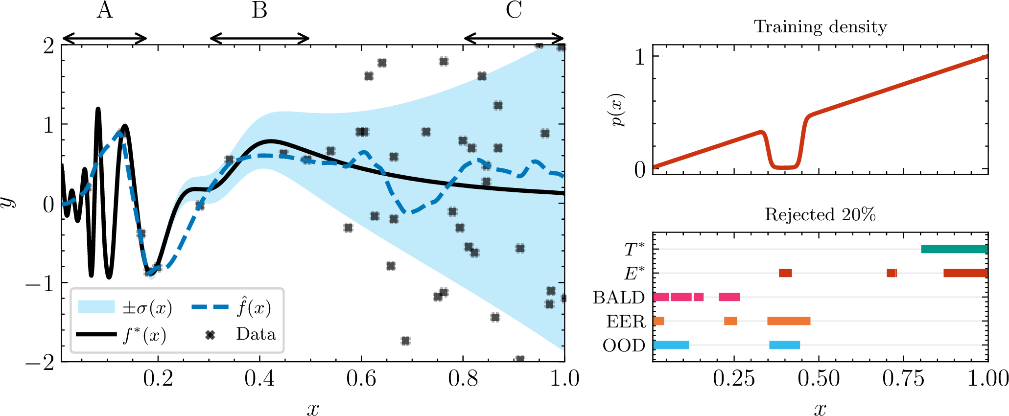
As visualised in 1, evaluating the exact Bayes-optimal scorers for OOD detection, EER, BALD, risk-coverage (\(T^{*}_{\ell}\)), and regret-coverage (\(E^{*}_{\ell}\)) at a fixed \(80\%\) coverage budget results in vastly different rejection behaviors. The scorers prioritize different subsets of the input space. This closed-form example confirms that evaluating an uncertainty method via OOD detection or active learning is not merely a noisy approximation of regret; it actively optimizes for rejecting a different subset of the data. The risk-coverage and regret-coverage rules, while distinct here, are not unrelated; rather, they form the boundary cases of a single constrained family, which we formalize next.
5 A Unified Constrained-Optimization Framework↩︎
Having established that proxy tasks fail to align with pure epistemic regret, a secondary evaluation challenge arises: how should we evaluate models that output both aleatoric (\(\hat{A}_{\ell}\)) and epistemic (\(\hat{E}_{\ell}\)) components? Recent literature attempts to evaluate the quality of these joint representations by measuring their rank correlation, arguing that high correlation indicates a failure of uncertainty disentanglement [3]. We provide a complementary diagnostic by measuring the operational utility of the scores. As we demonstrate empirically in 6, highly correlated components can still combine to form close-to-optimal rejection strategies. To properly evaluate this joint operational utility rather than mere statistical independence, we must first mathematically define how risk and regret trade off against each other under an optimal decision rule.
5.1 Three constrained problems, one selector↩︎
Consider three constrained-optimization problems over selectors \(C\colon \mathcal{X}\to [0,1]\), subject to budgets \(\rho, \gamma > 0\) and a coverage floor \(\kappa \in (0,1)\): \[\begin{align} (\mathrm{P}_{\rho}):\quad & \max_{C}\; \rho(C) \;\;\text{s.t.}\;\; Ri(C) \leq \rho,\; Re(C) \leq \gamma, \tag{4}\\ (\mathrm{P}_{Ri}):\quad & \min_{C}\; Ri(C) \;\;\text{s.t.}\;\; \rho(C) \geq \kappa,\; Re(C) \leq \gamma, \tag{5}\\ (\mathrm{P}_{Re}):\quad & \min_{C}\; Re(C) \;\;\text{s.t.}\;\; \rho(C) \geq \kappa,\; Ri(C) \leq \rho. \tag{6} \end{align}\]
Theorem 1 (Unified selector). Assume \(T^{*}_{\ell}(\cdot, \mathcal{D}), E^{*}_{\ell}(\cdot, \mathcal{D}) \in L^{1}(p^{*})\), and that for every \(\lambda \in [\frac{1}{2}, 1]\) the score \((1-\lambda)A^{*}_{\ell}+ \lambda E^{*}_{\ell}\) has a continuous distribution under \(x \sim p^{*}\). For any feasible instance of 4 , 5 , or 6 , there exist \(\lambda \in [\frac{1}{2}, 1]\) and \(\tau \in \mathbb{R}\) such that the optimal selector is: \[C^{*}(x) \;=\; \mathbf{1}\!\set{(1-\lambda)\,A^{*}_{\ell}(x) + \lambda\,E^{*}_{\ell}(x, \mathcal{D}) \;\leq\; \tau}. \label{eq:unified-selector}\tag{7}\] The endpoints recover the standard formulations: \(\lambda = \frac{1}{2}\) thresholds total uncertainty \(T^{*}_{\ell}= A^{*}_{\ell}+ E^{*}_{\ell}\) (selective prediction [6], [7]), while \(\lambda = 1\) thresholds epistemic uncertainty \(E^{*}_{\ell}\) alone (epistemic reject-option [14]).
Proof. The proof simply applies the [29], [30] KKT conditions to the Lagrangian of each problem. Full case-by-case algebra is provided in the Appendix. ◻
5.1.0.1 Remarks.
The theoretical bound \(\lambda \in [\frac{1}{2}, 1]\) applies strictly to the ground-truth components \(( A^{*}_{\ell}, E^{*}_{\ell})\). When evaluating imperfect learned estimators \((\hat{A}_{\ell}, \hat{E}_{\ell})\) empirically to construct achievable surfaces, we permit unconstrained linear combinations to compensate for miscalibration. Additionally, for non-strictly-proper losses (e.g., \(0/1\)), 1 holds almost everywhere; ties are handled via standard linear programming constructions [10].
5.2 A diagnostic for joint operational utility↩︎
Theorem 1 characterizes the optimal selector as a threshold on \((1-\lambda) {\small A^{*}_{\ell}} + \lambda {\small E^{*}_{\ell}}\), which traces a Pareto-optimal surface \(\mathcal{S}^\ast\) in \((\rho(C), Ri(C), Re(C))\)-space as \(\lambda\) sweeps \([\frac{1}{2}, 1]\). For learned estimators \((\hat{A}_{\ell}, \hat{E}_{\ell})\), the analogous achievable surface \(\mathcal{S}\) either matches \(\mathcal{S}^\ast\) closely or does not, and the distance between them quantifies whether the components jointly contain the information needed for optimal deployment decisions. We therefore propose this distance — the Pareto-gap — as a complementary diagnostic to rank correlation [3] for evaluating uncertainty decompositions.
We define the Pareto-optimal surface \(\mathcal{S}^{*}\) and a method’s achievable surface \(\mathcal{S}(\hat{A}_{\ell}, \hat{E}_{\ell})\) in the 3D space of Coverage (\(\rho\)), Risk (\(Ri\)), and Regret (\(Re\)): \[\begin{align} \mathcal{S}^{*} \;&=\; \big\{ (\rho(C), Ri(C), Re(C)) \;\big|\; C = \mathbf{1}\!\set{(1-\lambda) A^{*}_{\ell}+ \lambda E^{*}_{\ell}\leq \tau},\; \lambda \in[\frac{1}{2}, 1],\, \tau \in \mathbb{R}\big\}, \nonumber \\ \mathcal{S}(\hat{A}_{\ell}, \hat{E}_{\ell}) \;&=\; \big\{ (\rho(C), Ri(C), Re(C)) \;\big|\; C = \mathbf{1}\!\set{w_1 \hat{A}_{\ell}+ w_2 \hat{E}_{\ell}\leq \tau},\; w_1, w_2, \tau \in \mathbb{R}\big\}. \end{align}\] To analyze the best-case, in 6 we search for the optimal linear combination weights \((w_1, w_2)\) and thresholds \(\tau\) directly on the test set. We emphasize that this is an oracle evaluation designed to measure the total capacity of the estimated uncertainty, not a practical deployment strategy. We quantify the distance between a method achievable surface and the oracle surface using the Pareto-gap, calculated via the modified Inverted Generational Distance (IGD+) [31].
6 Empirical Benchmark↩︎
To validate our theoretical claims, we benchmark a diverse suite of uncertainty quantification methods. We implement and evaluate the proposed expected regret framework. For the standard proxy tasks—OOD detection, selective classification, and active
learning—we directly report the results from a concurrent submission probly [32] (provided in the supplementary material).
6.1 Experimental Setup↩︎
6.1.0.1 Datasets.
Our evaluation spans two regimes. First, for benchmarking the regret, we require datasets that provide access to a close approximation of the true data-generating distribution \(p^{*}(y \mid x)\) via dense human annotations1. We evaluate our framework on APPA-REAL [5] and the 8 diverse, real-world datasets2 comprising the DCIC benchmark suite [33] and CIFAR-10H [4]. Access to these dense distributions allows us to compute the exact Bayes-optimal predictor and the true regret across a variety of tasks and domains. Second, to evaluate standard proxy tasks, we use out-of-distribution detection on the OpenOOD benchmark [34], and active learning acquisition on OpenML [35] tabular dataset. We adopt the results on these proxies from a concurrent submission [32] (provided in the supplementary material).
6.1.0.2 Evaluated methods and implementation.
We evaluate a representative set of standard UQ baselines, spanning Bayesian, ensemble, and post-hoc families. These include MC-Dropout [36], Deep Ensembles [37], Deep Deterministic Uncertainty (DDU) [38] and Evidential Networks [39]. For CIFAR-10H and the DCIC suite, all methods utilize a ResNet-18 backbone pre-trained on ImageNet and fine-tuned on the respective target datasets. For the APPA-REAL age estimation task, we extract features using a ResNet-101 pre-trained on public facial age datasets, and train a lightweight MLP on top. Crucially, we treat all tasks as categorical probability estimation; APPA-REAL models are trained via Cross-Entropy over discrete age classes (0–100). However, as we define uncertainty strictly under the deployment loss \(\ell\), we extract the loss-consistent aleatoric (\(\hat{A}_{\ell}\)) and epistemic (\(\hat{E}_{\ell}\)) components under CE and 0/1 losses for CIFAR/DCIC, and under squared and absolute error losses for APPA-REAL [14], [20]. Full training details are provided in the Appendix.
6.2 Evaluation protocol and metrics↩︎
We evaluate the models along two distinct operational axes: pure epistemic utility of \(\hat{E}_{\ell}\) and joint representational capacity of both uncertainty estimates \(\hat{A}_{\ell}, \hat{E}_{\ell}\).
First, to evaluate pure epistemic utility, we fix the selector to threshold only the estimated epistemic component (\(\hat{E}_{\ell}\)). Let \(C_\rho\) be a selector that accepts the subset \(\mathcal{A}_\rho\) of \(\lfloor \rho N \rfloor\) points where \(\rho\in [0, 1]\) is the coverage. The generalized risk and regret curves [13] are \(Ri(\rho) \triangleq\frac{1}{N} \sum_{i \in \mathcal{A}_\rho} T^{*}_{\ell}(x_i, \mathcal{D})\) and \(Re(\rho) \triangleq\frac{1}{N} \sum_{i \in \mathcal{A}_\rho} E^{*}_{\ell}(x_i, \mathcal{D})\). We evaluate the realized frequentist counterparts of \(T^{*}_{\ell},A^{*}_{\ell},E^{*}_{\ell}\) but for brevity do not change notation.
Integrating these curves yields the area metrics \(\mathrm{AuRC}\) and \(\mathrm{AuReC}\triangleq\int_0^1 Re(\rho) \, d\rho\). To isolate the ranking quality of the selector from the inherent error differences of the classifiers, we define \(\text{excess-}\mathrm{AuReC}\triangleq\mathrm{AuReC}- \mathrm{AuReC}_{\text{oracle}}\) [40], and \(n\text{-}\mathrm{AuReC}\triangleq\frac{\mathrm{AuReC}- \mathrm{AuReC}_{\text{oracle}}}{\mathrm{AuReC}_{\text{random}} - \mathrm{AuReC}_{\text{oracle}}}\) [41]. Here, \(\mathrm{AuReC}_{\text{oracle}}\) is the area achieved by perfectly ranking points by \(E^{*}_{\ell}\), and \(\mathrm{AuReC}_{\text{random}}\) is the area of a random selector.
Second, to evaluate the operational disentanglement of \(\hat{A}_{\ell}\) and \(\hat{E}_{\ell}\), we measure how closely the method can approximate the theoretical optimum of 1. To this end, we measure the Pareto-gap, a distance between the achievable surface \(\mathcal{S}\) and the optimal surface \(\mathcal{S}^\ast\), see 5.
6.3 Results: Misalignment between proxy tasks and true regret↩︎
6.3.0.1 OOD detection.
A prevalent assumption in current literature is that improved OOD detection acts as a reliable surrogate for better epistemic uncertainty quantification. We now demonstrate empirically that the theoretical misalignment between the tasks (4) leads to rank inversions among standard UQ methods. We evaluate OOD detection \(\mathrm{AuROC}\) using the OpenOOD benchmark [34] (4) and epistemic regret using the \(\mathrm{AuReC}\) metric on datasets with dense human annotations ([tab:regret_cifar10h,tab:regret_appareal,tab:regret_dcic]). Under the proxy OOD task, Deep Ensembles and DDU are the dominant methods. On CIFAR-10, Deep Ensembles performs the best at Near-OOD (\(\mathrm{AuROC}=0.907\)), and DDU the best on Far-OOD (\(\mathrm{AuROC}=0.935\)). In contrast, Evidential networks perform poorly on these OOD splits, \(0.711\) and \(0.726\), respectively.
However, when evaluating strictly the ability to isolate the reducible error (regret) on the predictive task, the rankings shift markedly for individual methods. On CIFAR-10H (1, CE Loss), Evidential networks outperform all other baselines, yielding the lowest \(\mathrm{AuReC}= 0.0673\) and the best ranking quality isolated from base accuracy \(\text{ex-}\mathrm{AuReC}= 0.0183\). Conversely, DDU, which excelled at Far-OOD detection, performs the worst in terms of pure regret (\(\mathrm{AuReC}= 0.0958\)). Ultimately, relying on OOD detection as a proxy leads practitioners to select different models than if they directly measured deployment regret.
6.3.0.2 Active learning.
Beyond OOD detection, active learning is frequently utilized as a proxy benchmark for epistemic uncertainty estimators. To determine whether performance on this global acquisition task translates to our regret framework, we again report the active learning evaluations conducted by a concurrent submission [32] (provided in the supplementary material).
As shown in 5, when evaluating the Normalized Area Under the budget Curve (NAUC) on tabular datasets, MC-Dropout and Deep Ensembles reliably identify informative samples. Conversely, Evidential networks struggle significantly (e.g., \(0.177\) NAUC on OpenML 6). However, this ranking can invert when evaluating based on the regret, 1, for instance they dominate in epistemic regret on CIFAR-10H (\(\mathrm{AuReC}= 0.0673\)). This supports the theoretical claim from 4: selecting data to minimize expected future error globally operates under different mathematical incentives than isolating the reducible error of a specific sample.
6.4 Results: Rank correlation vs. operational disentanglement↩︎
Recent benchmarks rely on the Spearman rank correlation (\(r_s\)) to evaluate uncertainty disentanglement, asserting that highly correlated components (\(\hat{A}_{\ell}, \hat{E}_{\ell}\)) signify a failure to separate aleatoric and epistemic uncertainties [3]. However, our empirical evaluation reveals two issues with relying on this metric.
First, 1 shows that the rank correlation \(r_s(A^{*}_{\ell}, E^{*}_{\ell})\) of the ground-truth uncertainties on CIFAR-10H (with CE loss) reaches up to \(0.882\). Note that this ground-truth value varies across the evaluated methods because our definition of true epistemic uncertainty (\(E^{*}_{\ell}\)) evaluates the expected regret (reducible error) of the specific predictor being deployed. Consequently, a high rank correlation between learned estimators may accurately reflect the underlying data-generating process, rather than a failure of the uncertainty estimation method.
Second, rank correlation merely measures whether two scores sort the data in the same order; it does not capture their joint operational utility. For example, on CIFAR-10H (CE loss), Evidential networks exhibit a near-perfect rank correlation of \(r_s(\hat{A}_{\ell}, \hat{E}_{\ell}) = 0.999\), which would traditionally classify them as entirely entangled. Yet, when evaluating their joint representational capacity, Evidential network uncertainty estimates achieve the lowest distance to their theoretical optimum (\(\text{P-gap} = 0.0379\)) alongside the best pure epistemic utility (\(\mathrm{AuReC}= 0.0673\)).
This is possible because the unified framework (5) evaluates the achievable decision boundary \(\mathbf{1}\!\set{w_1 \hat{A}_{\ell}+ w_2 \hat{E}_{\ell}\leq \tau}\). Even if two components sort the data identically, unconstrained linear combinations of these scores can still form distinct decision boundaries, provided their relationship is not strictly linear. A low Pareto-gap directly implies that a linear combination of the estimated scores (\(\hat{A}_{\ell}, \hat{E}_{\ell}\)) can closely match the theoretically optimal decision boundary produced by \((A^{*}_{\ell}, E^{*}_{\ell})\) for any given budget of risk, coverage, and regret. Therefore, we propose the Pareto-gap as a more reliable diagnostic for disentanglement: it explicitly evaluates whether the components functionally contain the information needed to make optimal deployment decisions, rather than penalizing them for possibly correct correlation.
| Method | Loss | \(\downarrow\) \(\AuReC\) | \(\downarrow\) ex-\(\AuReC\) | \(\downarrow\) \(n\)-\(\AuReC\) | \(\downarrow\) \(\AuRC\) | \(\downarrow\) P-gap | \(r_s(\Ahat, \Ehat)\) | \(r_s(\Astar, \Estar)\) |
|---|---|---|---|---|---|---|---|---|
| Dropout | CE | \(0.1023\) | \(0.0738\) | \(0.592\) | \(0.1609\) | \(0.1074\) | \(0.912\) | \(0.882\) |
| \(0/1\) | \(0.0162\) | \(0.0154\) | \(0.852\) | \(0.0380\) | \(0.0117\) | \(0.205\) | \(0.216\) | |
| Evidential | CE | \(\mathbf{0.0673}\) | \(\mathbf{0.0183}\) | \(\mathbf{0.260}\) | \(\mathbf{0.1211}\) | \(\mathbf{0.0379}\) | \(0.999\) | \(0.293\) |
| \(0/1\) | \(\mathbf{0.0030}\) | \(\mathbf{0.0023}\) | \(\mathbf{0.132}\) | \(\mathbf{0.0175}\) | \(\underline{0.0103}\) | \(0.999\) | \(0.213\) | |
| Ensemble | CE | \(\underline{0.0752}\) | \(\underline{0.0491}\) | \(\underline{0.519}\) | \(\underline{0.1271}\) | \(\underline{0.0753}\) | \(0.880\) | \(0.865\) |
| \(0/1\) | \(0.0058\) | \(0.0053\) | \(0.379\) | \(0.0248\) | \(\mathbf{0.0097}\) | \(0.456\) | \(0.208\) | |
| DDU | CE | \(0.0958\) | \(0.0665\) | \(0.543\) | \(0.1520\) | \(0.0979\) | \(0.674\) | \(0.875\) |
| \(0/1\) | \(\underline{0.0034}\) | \(\underline{0.0027}\) | \(0.151\) | \(\underline{0.0188}\) | \(0.0108\) | \(0.678\) | \(0.212\) |
| Method | Loss | \(\downarrow\) \(\AuReC\) | \(\downarrow\) ex-\(\AuReC\) | \(\downarrow\) \(n\)-\(\AuReC\) | \(\downarrow\) \(\AuRC\) | \(\downarrow\) P-gap | \(r_s(\Ahat, \Ehat)\) | \(r_s(\Astar, \Estar)\) |
|---|---|---|---|---|---|---|---|---|
| Dropout | sqr | \(\underline{11.6382}\) | \(\mathbf{6.6169}\) | \(\underline{0.418}\) | \(\mathbf{22.6765}\) | \(0.2005\) | \(0.823\) | \(0.316\) |
| abs | \(\underline{0.8184}\) | \(\mathbf{0.4499}\) | \(\mathbf{0.618}\) | \(\mathbf{2.5493}\) | \(0.1722\) | \(0.718\) | \(0.133\) | |
| Evidential | sqr | \(16.9411\) | \(8.4294\) | \(\mathbf{0.386}\) | \(30.5462\) | \(0.1998\) | \(0.976\) | \(-0.128\) |
| abs | \(0.9707\) | \(0.5689\) | \(0.713\) | \(2.7757\) | \(0.1678\) | \(0.418\) | \(0.049\) | |
| Ensemble | sqr | \(\mathbf{11.3519}\) | \(\underline{6.6908}\) | \(0.453\) | \(\underline{22.8190}\) | \(\mathbf{0.1806}\) | \(0.674\) | \(0.273\) |
| abs | \(\mathbf{0.7948}\) | \(\underline{0.4640}\) | \(\underline{0.689}\) | \(\underline{2.5685}\) | \(\mathbf{0.1531}\) | \(0.580\) | \(0.107\) | |
| DDU | sqr | \(20.0456\) | \(15.4126\) | \(1.048\) | \(33.5724\) | \(\underline{0.1843}\) | \(-0.201\) | \(0.273\) |
| abs | \(1.0422\) | \(0.7116\) | \(1.048\) | \(3.0234\) | \(\underline{0.1595}\) | \(-0.235\) | \(0.104\) |
| Method | Loss | \(\uparrow\) Best | \(\downarrow\) \(\overline{n\text{-}\AuReC}\) | \(\downarrow\) \(\overline{\text{P-gap}}\) | \(\overline{r_s(\Ahat, \Ehat)}\) | \(\overline{r_s(\Astar, \Estar)}\) | |
|---|---|---|---|---|---|---|---|
| MC-Dropout | CE | 0 | \(0.688\) | \(0.0478\) | \(0.601\) | \(0.292\) | |
| \(0/1\) | 0 | \(0.794\) | \(0.0237\) | \(0.484\) | \(0.267\) | ||
| Evidential | CE | 3 | \(\underline{0.601}\) | \(\mathbf{0.0362}\) | \(0.521\) | \(0.208\) | |
| \(0/1\) | 2 | \(\underline{0.617}\) | \(\underline{0.0226}\) | \(0.461\) | \(0.277\) | ||
| Ensemble | CE | 5 | \(\mathbf{0.596}\) | \(\underline{0.0385}\) | \(0.651\) | \(0.291\) | |
| \(0/1\) | 6 | \(\mathbf{0.502}\) | \(\mathbf{0.0207}\) | \(0.594\) | \(0.289\) | ||
| DDU | CE | 0 | \(0.967\) | \(0.0572\) | \(-0.219\) | \(0.347\) | |
| \(0/1\) | 0 | \(0.978\) | \(0.0248\) | \(-0.216\) | \(0.266\) |
| CIFAR10 | Imagenet | |||||
|---|---|---|---|---|---|---|
| 2-4 (lr)5-7 Method | \(\uparrow\) Near-OOD | \(\uparrow\) Far-OOD | \(\uparrow\) \(\AuAC\) | \(\uparrow\) Near-OOD | \(\uparrow\) Far-OOD | \(\uparrow\) \(\AuAC\) |
| DDU | 0.899 | 0.935 | 0.995 | 0.673 | 0.803 | 0.916 |
| Dropout | 0.839 | 0.895 | 0.990 | 0.690 | 0.761 | 0.916 |
| Ensemble | 0.907 | 0.931 | 0.997 | 0.737 | 0.820 | 0.935 |
| Evidential | 0.711 | 0.726 | 0.901 | 0.719 | 0.700 | 0.816 |
| OpenML ID 6 | OpenML ID 156 | |||
|---|---|---|---|---|
| 2-3 (lr)4-5 Method | EU \(\uparrow\) | TU \(\uparrow\) | EU \(\uparrow\) | TU \(\uparrow\) |
| MC-Dropout | 0.962 | 0.963 | 0.655 | 0.822 |
| Deep Ensemble | 0.960 | 0.959 | 0.783 | 0.857 |
| DDU | 0.943 | 0.956 | 0.693 | 0.839 |
| Evidential | 0.177 | 0.177 | 0.606 | 0.606 |
7 Conclusion and Limitations↩︎
In this work, we addressed an evaluation misalignment in uncertainty quantification. We demonstrated that standard proxy tasks—such as out-of-distribution detection and active learning—optimize objectives that are mathematically distinct from minimizing deployment regret. We unified selective classification and the epistemic reject-option into a single constrained-optimization framework. We show that rank correlation between learned aleatoric and epistemic components is largely blind to their joint operational utility. We benchmarked methods by their pure epistemic utility (\(\mathrm{AuReC}\)) and their joint representational capacity (the Pareto-gap).
7.0.0.1 Limitations & broader impact.
Calculating true expected regret requires access to the exact data-generating distribution \(p^{*}(y \mid x)\). Consequently, the used metrics are strictly benchmarking tools and cannot single-label data. Due to the use of data with \(p^{*}(y \mid x)\), our ground-truth operational regret is computed against the unrestricted oracle and explicitly contains both estimation and approximation error. However, we do not separate them. Our evaluations span heterogeneous datasets; different datasets for OOD, active learning, and regret. This work constitutes research on the evaluation of machine learning reliability. We do not foresee any negative societal impacts.
Appendix: Evaluating Epistemic Uncertainty
8 Proof of 1↩︎
We solve the constrained optimization problems \((P_{\rho})\), \((P_{Ri})\), and \((P_{Re})\) using the method of Lagrange multipliers and the Karush-Kuhn-Tucker (KKT) conditions [29], [30].
Because we operate in the fixed-dataset regime (as defined in Section 3), the training dataset \(\mathcal{D}\) is given, and the true uncertainty components \(T^{*}_{\ell}(\cdot, \mathcal{D})\), \(A^{*}_{\ell}(\cdot, \mathcal{D})\), and \(E^{*}_{\ell}(\cdot, \mathcal{D})\) are deterministic functions of the input \(x\). Consequently, our metrics are defined as expectations strictly over the marginal test distribution \(p^{*}(x)\). Identical results hold when the metrics are defined over the \(p^{*}(x, \mathcal{D})\).
8.0.0.1 Case 1: (\(P_{\rho}\)) Maximizing Coverage.
Our goal is to maximize \(\rho(C)\), which is equivalent to minimizing \(-\rho(C)\). Let \(\alpha \ge 0\) be the multiplier for the risk constraint (\(Ri(C) \le \rho\)) and \(\beta \ge 0\) be the multiplier for the regret constraint (\(Re(C) \le \gamma\)). The Lagrangian is: \[\mathcal{L}_{\rho} \;=\; -\rho(C) + \alpha \big(Ri(C) - \rho\big) + \beta \big(Re(C) - \gamma\big)\] Expanding the metrics into their expectations and substituting \(T^{*}_{\ell}(x, \mathcal{D}) = A^{*}_{\ell}(x, \mathcal{D}) + E^{*}_{\ell}(x, \mathcal{D})\), we group all terms multiplied by \(C(x)\): \[\mathcal{L}_{\rho} \;=\; \mathop{\mathrm{\mathbb{E}}}_{x \sim p^{*}}\big[C(x)\, \big(-1 + \alpha A^{*}_{\ell}(x, \mathcal{D}) + (\alpha + \beta) E^{*}_{\ell}(x, \mathcal{D})\big)\big] - \alpha\rho - \beta\gamma\] Setting the inner term to be less than or equal to zero gives the decision rule: \[\alpha A^{*}_{\ell}(x, \mathcal{D}) + (\alpha + \beta) E^{*}_{\ell}(x, \mathcal{D}) \le 1\] Dividing by \(2\alpha + \beta\) expresses this as a convex combination: \[(1 - \lambda)\, A^{*}_{\ell}(x, \mathcal{D}) + \lambda\, E^{*}_{\ell}(x, \mathcal{D}) \le \tau\] where \(\lambda \triangleq\frac{\alpha+\beta}{2\alpha+\beta}\) and \(\tau \triangleq\frac{1}{2\alpha+\beta}\). Because \(\alpha \ge 0\) and \(\beta \ge 0\), the numerator of \(\lambda\) is always at least half of its denominator. Therefore, \(\lambda \in [1/2, 1]\).
8.0.0.2 Case 2: (\(P_{Ri}\)) Minimizing Risk.
Our goal is to minimize \(Ri(C)\). Let \(\alpha \ge 0\) be the multiplier for the coverage floor (\(\kappa - \rho(C) \le 0\)) and \(\beta \ge 0\) be the multiplier for the regret constraint (\(Re(C) - \gamma \le 0\)). The Lagrangian is: \[\mathcal{L}_{Ri} \;=\; Ri(C) + \alpha \big(\kappa - \rho(C)\big) + \beta \big(Re(C) - \gamma\big)\] Grouping the terms multiplied by \(C(x)\) gives: \[\mathcal{L}_{Ri} \;=\; \mathop{\mathrm{\mathbb{E}}}_{x \sim p^{*}}\big[C(x)\, \big(A^{*}_{\ell}(x, \mathcal{D}) + (1 + \beta) E^{*}_{\ell}(x, \mathcal{D}) - \alpha\big)\big] + \alpha\kappa - \beta\gamma\] Setting the inner term to be less than or equal to zero yields: \[A^{*}_{\ell}(x, \mathcal{D}) + (1 + \beta) E^{*}_{\ell}(x, \mathcal{D}) \le \alpha\] Dividing by \(2 + \beta\) gives the optimal thresholding rule with: \[\lambda \triangleq\frac{1+\beta}{2+\beta}, \quad \tau \triangleq\frac{\alpha}{2+\beta}\] The smallest value for \(\lambda\) occurs when \(\beta = 0\), giving \(\lambda = 1/2\). As \(\beta \to \infty\), \(\lambda\) approaches \(1\). Therefore, \(\lambda \in[1/2, 1)\).
8.0.0.3 Case 3: (\(P_{Re}\)) Minimizing Regret.
Our goal is to minimize \(Re(C)\). Let \(\alpha \ge 0\) be the multiplier for the coverage floor (\(\kappa - \rho(C) \le 0\)) and \(\beta \ge 0\) be the multiplier for the risk constraint (\(Ri(C) - \rho \le 0\)). The Lagrangian is: \[\mathcal{L}_{Re} \;=\; Re(C) + \alpha \big(\kappa - \rho(C)\big) + \beta \big(Ri(C) - \rho\big)\] Grouping the terms multiplied by \(C(x)\) gives: \[\mathcal{L}_{Re} \;=\; \mathop{\mathrm{\mathbb{E}}}_{x \sim p^{*}}\big[C(x)\, \big(\beta A^{*}_{\ell}(x, \mathcal{D}) + (1 + \beta) E^{*}_{\ell}(x, \mathcal{D}) - \alpha\big)\big] + \alpha\kappa - \beta\rho\] Setting the inner term to be less than or equal to zero yields: \[\beta A^{*}_{\ell}(x, \mathcal{D}) + (1 + \beta) E^{*}_{\ell}(x, \mathcal{D}) \le \alpha\] Dividing by \(1 + 2\beta\) gives: \[\lambda \triangleq\frac{1+\beta}{1+2\beta}, \quad \tau \triangleq\frac{\alpha}{1+2\beta}\] The largest value for \(\lambda\) occurs when \(\beta = 0\), giving \(\lambda = 1\). As \(\beta \to \infty\), the fraction approaches \(1/2\). Therefore, \(\lambda \in (1/2, 1]\).
8.0.0.4 Summary.
In all feasible instances across the three optimization problems, the optimal selector forms a threshold on a convex combination \((1-\lambda)A^{*}_{\ell}(x, \mathcal{D}) + \lambda E^{*}_{\ell}(x, \mathcal{D})\) where the weighting parameter \(\lambda\) is strictly bounded in \([1/2, 1]\). Note that he theoretical bound applies strictly to the ground-truth components \((A^{*}_{\ell}, E^{*}_{\ell})\), not to imperfect learned estimators \((\hat{A}_{\ell}, \hat{E}_{\ell})\).
\(\square\)
9 Proof of Theorem 1 under Normalized Metrics↩︎
We define the normalized (selective) risk and regret metrics as ratios of their expected values over the coverage: \[SRi(C) \triangleq\frac{Ri(C)}{\rho(C)}, \qquad SRe(C) \triangleq\frac{Re(C)}{\rho(C)}\]
We can avoid redundantly solving the three optimization cases by observing that the unnormalized optimization problems from Section 8 all share a generalized Lagrangian of the form: \[\mathcal{L} \;=\; c_1 \cdot Ri(C) + c_2 \cdot Re(C) - d \cdot \rho(C) + \text{Constants} \label{eq:general95unnormalized}\tag{8}\] where \(c_1 \ge 0\) and \(c_2 \ge 0\) are either \(1\) (if the metric is the objective) or a Lagrange multiplier \(\alpha, \beta \ge 0\) (if the metric is a constraint), and \(d\) absorbs the coverage constraints and objectives. Substituting \(T^{*}_{\ell}(x, \mathcal{D}) = A^{*}_{\ell}(x, \mathcal{D}) + E^{*}_{\ell}(x, \mathcal{D})\), the point-wise decision rule for this generalized Lagrangian is to accept when: \[c_1\, A^{*}_{\ell}(x, \mathcal{D}) + (c_1 + c_2)\, E^{*}_{\ell}(x, \mathcal{D}) \le d \quad \implies \quad (1 - \lambda)A^{*}_{\ell}(x, \mathcal{D}) + \lambda E^{*}_{\ell}(x, \mathcal{D}) \le \tau \label{eq:lambda95mapping}\tag{9}\] where the trade-off parameter defining the convex combination is \(\lambda \triangleq\frac{c_1+c_2}{2c_1+c_2} \in [1/2, 1]\).
We now show that substituting the normalized metrics \(SRi(C)\) and \(SRe(C)\) into the original problems simply transforms them back into the exact same generalized Lagrangian, preserving \(c_1\) and \(c_2\). Because the optimization acts over fractional metrics and \(\rho(C) > 0\), we apply linear-fractional programming techniques:
Fractional Constraints: Any constraint on a normalized metric with an arbitrary budget bound \(b\), such as \(SRi(C) \le b\), is algebraically linearized by multiplying by the coverage, yielding \(Ri(C) - b\,\rho(C) \le 0\). If this constraint has a Lagrange multiplier \(\alpha\), its contribution to the Lagrangian becomes \(\alpha Ri(C) - \alpha b\,\rho(C)\).
Fractional Objectives: To minimize a fractional objective like \(SRi(C)\), we apply Dinkelbach’s theorem [47]. If \(C^*\) is the optimal selector yielding a minimum ratio \(q^* = SRi(C^*)\), then \(C^*\) equivalently minimizes the linearized objective \(Ri(C) - q^* \rho(C)\).
Applying these linearizations to any of the three optimization problems transforms the fractional metrics into their unnormalized counterparts, minus a coverage penalty. Collecting the terms yields a new Lagrangian: \[\mathcal{L}_{norm} \;=\; c_1 \cdot Ri(C) + c_2 \cdot Re(C) - d' \cdot \rho(C) + \text{Constants}\] Crucially, the coefficients \(c_1\) and \(c_2\) scaling the risk and regret are identically the same as in the unnormalized case. The fractional linearizations only alter the coefficient on the coverage term, shifting \(d\) to \(d'\) (which absorbs the budget bounds and optimal ratio penalties like \(b\) and \(q^*\)).
Because \(\lambda\) strictly depends only on \(c_1\) and \(c_2\) (Equation 9 ), the trade-off parameter between aleatoric and epistemic uncertainty remains. The use of normalized metrics purely shifts the optimal operating threshold \(\tau\), but the functional form of the boundary \(\lambda \in [1/2, 1]\) remains identical. \(\square\)
10 Implementation Details↩︎
All base model training, uncertainty extraction, and metric evaluations were executed using the standardized UQ framework probly [32]. We
implemented our novel decision-theoretic regret evaluations (AuReC, Pareto-gap) on top of this framework.
10.1 Datasets and Architectures↩︎
10.1.0.1 CIFAR-10H.
Models were trained on the standard 50,000-image CIFAR-10 training split and evaluated on the 10,000-image CIFAR-10H test set, which contains dense human soft-label annotations [4]. We utilized a ResNet-18 backbone trained from scratch for 200 epochs. Training included standard data augmentations.
10.1.0.2 DCIC Suite.
We evaluated on the multi-rater image classification datasets from the DCIC benchmark [33] (omitting the CIFAR-10H duplicate). For all DCIC datasets, we utilized a ResNet-18 backbone initialized with ImageNet-1K pre-trained weights. The classification head was replaced, and the networks were fine-tuned for 100 epochs.
10.1.0.3 APPA-REAL.
The APPA-REAL apparent age dataset [5] was treated as a discrete probability estimation task over integer ages \(0\) to \(100\) (\(K=101\)). To ensure high-quality representations, we extracted 2048-dimensional features using a ResNet-101 backbone pre-trained public facial age benchmarks [42]–[46]. The backbone was frozen, and a lightweight Multi-Layer Perceptron (MLP) head was trained in a probe regime. The MLP architecture consisted of a linear layer (128 hidden units), ReLU activation, dropout, and a final linear projection.
10.2 Method-Specific Training Regimes↩︎
Unless otherwise specified, methods evaluating on CIFAR-10H and DCIC utilized Stochastic Gradient Descent (SGD) with a learning rate of \(0.1\), Nesterov momentum of \(0.9\), weight decay of \(5\times 10^{-4}\), and a cosine annealing schedule. For the APPA-REAL feature-probe task, methods utilized AdamW with a learning rate of \(10^{-3}\) and weight decay of \(10^{-4}\) for 50 epochs. CIFAR-10 training utilizes one-hot labels, APPA-REAL and DCIC utilize the soft label distributions.
Deep Ensembles: Comprised of \(M=5\) independently initialized members. For APPA-REAL, members also utilized a deterministic 5-fold partition of the training pool (each member dropping a different fold) to inject data-side diversity.
MC-Dropout: Utilized dropout probabilities of \(p=0.1\) prior to linear layers. At inference, \(S=20\) stochastic forward passes were drawn.
Evidential Networks: The final layer utilized a
Softplus + 1activation to emit Dirichlet concentration parameters (\(\alpha\)). The models were trained using the soft-label evidential Cross-Entropy loss without the optional KL-divergence regularizer (\(\lambda_{KL} = 0\)).Deep Deterministic Uncertainty (DDU): Spectral normalization was applied to all hidden layers with a Lipschitz coefficient of \(3.0\), and activations were swapped to LeakyReLU. Following the initial Cross-Entropy training phase, a Gaussian Mixture Model (GMM) was fit to the spectrally-normalized pre-logit features to extract the marginal log-density.
11 Detailed Results↩︎
| Method | Loss | \(\AuReC\) | ex-\(\AuReC\) | \(n\)-\(\AuReC\) | \(\AuRC\) | P-gap | \(r_s(\Ahat, \Ehat)\) | \(r_s(\Astar, \Estar)\) |
|---|---|---|---|---|---|---|---|---|
| MC-Dropout | CE | \(\underline{0.1991}\) | \(0.1004\) | \(\underline{0.631}\) | \(\underline{0.3326}\) | \(0.0859\) | \(0.786\) | \(0.371\) |
| \(0/1\) | \(0.0492\) | \(0.0391\) | \(0.727\) | \(\underline{0.1312}\) | \(0.0389\) | \(0.526\) | \(0.200\) | |
| Evidential | CE | \(0.2285\) | \(\underline{0.0993}\) | \(0.712\) | \(0.3965\) | \(\mathbf{0.0734}\) | \(0.524\) | \(0.328\) |
| \(0/1\) | \(\underline{0.0468}\) | \(\underline{0.0377}\) | \(\underline{0.726}\) | \(0.1334\) | \(\underline{0.0384}\) | \(0.384\) | \(0.190\) | |
| Ensemble | CE | \(\mathbf{0.1732}\) | \(\mathbf{0.0887}\) | \(\mathbf{0.602}\) | \(\mathbf{0.3083}\) | \(\underline{0.0855}\) | \(0.806\) | \(0.415\) |
| \(0/1\) | \(\mathbf{0.0314}\) | \(\mathbf{0.0245}\) | \(\mathbf{0.537}\) | \(\mathbf{0.1061}\) | \(\mathbf{0.0335}\) | \(0.677\) | \(0.206\) | |
| DDU | CE | \(0.2973\) | \(0.2020\) | \(1.079\) | \(0.4876\) | \(0.1198\) | \(-0.267\) | \(0.453\) |
| \(0/1\) | \(0.0665\) | \(0.0567\) | \(1.055\) | \(0.1643\) | \(0.0398\) | \(-0.273\) | \(0.184\) |
| Method | Loss | \(\AuReC\) | ex-\(\AuReC\) | \(n\)-\(\AuReC\) | \(\AuRC\) | P-gap | \(r_s(\Ahat, \Ehat)\) | \(r_s(\Astar, \Estar)\) |
|---|---|---|---|---|---|---|---|---|
| MC-Dropout | CE | \(0.0814\) | \(0.0471\) | \(0.660\) | \(0.2010\) | \(0.0431\) | \(0.690\) | \(0.450\) |
| \(0/1\) | \(0.0306\) | \(0.0274\) | \(0.942\) | \(0.1043\) | \(0.0198\) | \(0.410\) | \(0.333\) | |
| Evidential | CE | \(\underline{0.0635}\) | \(\mathbf{0.0273}\) | \(\mathbf{0.501}\) | \(\underline{0.1755}\) | \(\mathbf{0.0260}\) | \(0.825\) | \(0.358\) |
| \(0/1\) | \(\mathbf{0.0154}\) | \(\mathbf{0.0128}\) | \(\mathbf{0.476}\) | \(\mathbf{0.0667}\) | \(\underline{0.0177}\) | \(0.795\) | \(0.330\) | |
| Ensemble | CE | \(\mathbf{0.0581}\) | \(\underline{0.0284}\) | \(\underline{0.517}\) | \(\mathbf{0.1653}\) | \(\underline{0.0273}\) | \(0.816\) | \(0.436\) |
| \(0/1\) | \(\underline{0.0161}\) | \(\underline{0.0137}\) | \(\underline{0.533}\) | \(\underline{0.0781}\) | \(\mathbf{0.0160}\) | \(0.635\) | \(0.337\) | |
| DDU | CE | \(0.1136\) | \(0.0805\) | \(1.169\) | \(0.3062\) | \(0.0424\) | \(-0.513\) | \(0.487\) |
| \(0/1\) | \(0.0391\) | \(0.0360\) | \(1.227\) | \(0.1301\) | \(0.0192\) | \(-0.494\) | \(0.314\) |
| Method | Loss | \(\AuReC\) | ex-\(\AuReC\) | \(n\)-\(\AuReC\) | \(\AuRC\) | P-gap | \(r_s(\Ahat, \Ehat)\) | \(r_s(\Astar, \Estar)\) |
|---|---|---|---|---|---|---|---|---|
| MC-Dropout | CE | \(0.1890\) | \(0.0816\) | \(0.955\) | \(\underline{0.5345}\) | \(0.0633\) | \(0.329\) | \(-0.133\) |
| \(0/1\) | \(\underline{0.0586}\) | \(\underline{0.0426}\) | \(\underline{0.801}\) | \(\underline{0.2238}\) | \(\underline{0.0503}\) | \(0.658\) | \(0.090\) | |
| Evidential | CE | \(\underline{0.1884}\) | \(\underline{0.0753}\) | \(\underline{0.874}\) | \(0.5535\) | \(\underline{0.0602}\) | \(0.199\) | \(-0.187\) |
| \(0/1\) | \(0.0663\) | \(0.0494\) | \(0.906\) | \(0.2387\) | \(0.0512\) | \(0.106\) | \(0.079\) | |
| Ensemble | CE | \(\mathbf{0.1638}\) | \(\mathbf{0.0637}\) | \(\mathbf{0.832}\) | \(\mathbf{0.5133}\) | \(\mathbf{0.0513}\) | \(0.302\) | \(-0.168\) |
| \(0/1\) | \(\mathbf{0.0469}\) | \(\mathbf{0.0333}\) | \(\mathbf{0.670}\) | \(\mathbf{0.2068}\) | \(\mathbf{0.0464}\) | \(0.565\) | \(0.099\) | |
| DDU | CE | \(0.1981\) | \(0.0807\) | \(0.879\) | \(0.5720\) | \(0.0715\) | \(-0.015\) | \(-0.109\) |
| \(0/1\) | \(0.0732\) | \(0.0533\) | \(0.910\) | \(0.2498\) | \(0.0556\) | \(-0.028\) | \(0.039\) |
| Method | Loss | \(\AuReC\) | ex-\(\AuReC\) | \(n\)-\(\AuReC\) | \(\AuRC\) | P-gap | \(r_s(\Ahat, \Ehat)\) | \(r_s(\Astar, \Estar)\) |
|---|---|---|---|---|---|---|---|---|
| MC-Dropout | CE | \(\underline{0.0499}\) | \(0.0306\) | \(\underline{0.403}\) | \(\underline{0.0872}\) | \(0.0401\) | \(0.975\) | \(0.613\) |
| \(0/1\) | \(0.0174\) | \(0.0164\) | \(0.840\) | \(0.0522\) | \(0.0101\) | \(0.280\) | \(0.322\) | |
| Evidential | CE | \(0.0791\) | \(\underline{0.0274}\) | \(0.440\) | \(0.1305\) | \(\mathbf{0.0254}\) | \(0.858\) | \(0.537\) |
| \(0/1\) | \(\underline{0.0084}\) | \(\underline{0.0076}\) | \(\underline{0.438}\) | \(\mathbf{0.0298}\) | \(0.0094\) | \(0.836\) | \(0.325\) | |
| Ensemble | CE | \(\mathbf{0.0393}\) | \(\mathbf{0.0240}\) | \(\mathbf{0.396}\) | \(\mathbf{0.0767}\) | \(\underline{0.0316}\) | \(0.949\) | \(0.629\) |
| \(0/1\) | \(\mathbf{0.0063}\) | \(\mathbf{0.0057}\) | \(\mathbf{0.416}\) | \(\underline{0.0333}\) | \(\mathbf{0.0076}\) | \(0.485\) | \(0.328\) | |
| DDU | CE | \(0.0760\) | \(0.0596\) | \(0.833\) | \(0.1533\) | \(0.0426\) | \(0.128\) | \(0.654\) |
| \(0/1\) | \(0.0137\) | \(0.0130\) | \(0.804\) | \(0.0457\) | \(\underline{0.0088}\) | \(0.125\) | \(0.332\) |
| Method | Loss | \(\AuReC\) | ex-\(\AuReC\) | \(n\)-\(\AuReC\) | \(\AuRC\) | P-gap | \(r_s(\Ahat, \Ehat)\) | \(r_s(\Astar, \Estar)\) |
|---|---|---|---|---|---|---|---|---|
| MC-Dropout | CE | \(0.0166\) | \(0.0114\) | \(1.084\) | \(0.2951\) | \(0.0111\) | \(-0.041\) | \(-0.089\) |
| \(0/1\) | \(\underline{0.0055}\) | \(\underline{0.0050}\) | \(0.780\) | \(\mathbf{0.1395}\) | \(\underline{0.0105}\) | \(0.668\) | \(0.304\) | |
| Evidential | CE | \(\mathbf{0.0122}\) | \(\mathbf{0.0070}\) | \(\mathbf{0.771}\) | \(\mathbf{0.2866}\) | \(\mathbf{0.0064}\) | \(0.143\) | \(-0.240\) |
| \(0/1\) | \(0.0061\) | \(0.0055\) | \(\underline{0.754}\) | \(0.1451\) | \(\mathbf{0.0082}\) | \(0.143\) | \(0.341\) | |
| Ensemble | CE | \(\underline{0.0152}\) | \(\underline{0.0094}\) | \(1.012\) | \(\underline{0.2875}\) | \(\underline{0.0083}\) | \(0.100\) | \(-0.142\) |
| \(0/1\) | \(\mathbf{0.0052}\) | \(\mathbf{0.0043}\) | \(\mathbf{0.381}\) | \(\underline{0.1400}\) | \(0.0107\) | \(0.608\) | \(0.361\) | |
| DDU | CE | \(0.0198\) | \(0.0121\) | \(\underline{0.905}\) | \(0.2983\) | \(0.0153\) | \(-0.149\) | \(-0.063\) |
| \(0/1\) | \(0.0141\) | \(0.0127\) | \(0.864\) | \(0.1559\) | \(0.0155\) | \(-0.149\) | \(0.277\) |
| Method | Loss | \(\AuReC\) | ex-\(\AuReC\) | \(n\)-\(\AuReC\) | \(\AuRC\) | P-gap | \(r_s(\Ahat, \Ehat)\) | \(r_s(\Astar, \Estar)\) |
|---|---|---|---|---|---|---|---|---|
| MC-Dropout | CE | \(0.1080\) | \(0.0576\) | \(0.497\) | \(\underline{0.1974}\) | \(0.0601\) | \(0.902\) | \(0.531\) |
| \(0/1\) | \(0.0340\) | \(0.0293\) | \(0.741\) | \(0.0807\) | \(0.0231\) | \(0.422\) | \(0.307\) | |
| Evidential | CE | \(\underline{0.1049}\) | \(\underline{0.0429}\) | \(\underline{0.478}\) | \(0.2183\) | \(\mathbf{0.0367}\) | \(0.681\) | \(0.464\) |
| \(0/1\) | \(\underline{0.0217}\) | \(\underline{0.0182}\) | \(\underline{0.539}\) | \(\underline{0.0697}\) | \(\underline{0.0198}\) | \(0.628\) | \(0.331\) | |
| Ensemble | CE | \(\mathbf{0.0797}\) | \(\mathbf{0.0383}\) | \(\mathbf{0.421}\) | \(\mathbf{0.1680}\) | \(\underline{0.0423}\) | \(0.889\) | \(0.553\) |
| \(0/1\) | \(\mathbf{0.0182}\) | \(\mathbf{0.0153}\) | \(\mathbf{0.495}\) | \(\mathbf{0.0596}\) | \(\mathbf{0.0177}\) | \(0.603\) | \(0.339\) | |
| DDU | CE | \(0.1490\) | \(0.1045\) | \(0.926\) | \(0.2977\) | \(0.0640\) | \(-0.159\) | \(0.597\) |
| \(0/1\) | \(0.0364\) | \(0.0326\) | \(0.918\) | \(0.1003\) | \(0.0204\) | \(-0.156\) | \(0.327\) |
| Method | Loss | \(\AuReC\) | ex-\(\AuReC\) | \(n\)-\(\AuReC\) | \(\AuRC\) | P-gap | \(r_s(\Ahat, \Ehat)\) | \(r_s(\Astar, \Estar)\) |
|---|---|---|---|---|---|---|---|---|
| MC-Dropout | CE | \(0.1027\) | \(0.0536\) | \(0.841\) | \(\underline{0.4568}\) | \(0.0418\) | \(0.235\) | \(0.163\) |
| \(0/1\) | \(0.0165\) | \(0.0144\) | \(0.684\) | \(\underline{0.1727}\) | \(0.0202\) | \(0.537\) | \(0.280\) | |
| Evidential | CE | \(\underline{0.0885}\) | \(\underline{0.0324}\) | \(\underline{0.608}\) | \(0.4914\) | \(\mathbf{0.0299}\) | \(0.085\) | \(0.080\) |
| \(0/1\) | \(\underline{0.0149}\) | \(\underline{0.0131}\) | \(\underline{0.678}\) | \(0.1969\) | \(\underline{0.0187}\) | \(-0.030\) | \(0.303\) | |
| Ensemble | CE | \(\mathbf{0.0770}\) | \(\mathbf{0.0304}\) | \(\mathbf{0.562}\) | \(\mathbf{0.4230}\) | \(\underline{0.0310}\) | \(0.485\) | \(0.188\) |
| \(0/1\) | \(\mathbf{0.0115}\) | \(\mathbf{0.0097}\) | \(\mathbf{0.507}\) | \(\mathbf{0.1640}\) | \(\mathbf{0.0181}\) | \(0.593\) | \(0.304\) | |
| DDU | CE | \(0.1030\) | \(0.0511\) | \(0.803\) | \(0.5308\) | \(0.0460\) | \(-0.386\) | \(0.234\) |
| \(0/1\) | \(0.0204\) | \(0.0179\) | \(0.808\) | \(0.2126\) | \(0.0217\) | \(-0.362\) | \(0.306\) |
| Method | Loss | \(\AuReC\) | ex-\(\AuReC\) | \(n\)-\(\AuReC\) | \(\AuRC\) | P-gap | \(r_s(\Ahat, \Ehat)\) | \(r_s(\Astar, \Estar)\) |
|---|---|---|---|---|---|---|---|---|
| MC-Dropout | CE | \(\underline{0.0574}\) | \(0.0295\) | \(0.432\) | \(\mathbf{0.1169}\) | \(0.0374\) | \(0.935\) | \(0.430\) |
| \(0/1\) | \(0.0277\) | \(0.0250\) | \(0.838\) | \(0.0689\) | \(\underline{0.0168}\) | \(0.375\) | \(0.300\) | |
| Evidential | CE | \(0.0677\) | \(\underline{0.0292}\) | \(\mathbf{0.426}\) | \(0.1369\) | \(\underline{0.0319}\) | \(0.851\) | \(0.325\) |
| \(0/1\) | \(\underline{0.0164}\) | \(\underline{0.0136}\) | \(\mathbf{0.417}\) | \(\mathbf{0.0457}\) | \(0.0173\) | \(0.828\) | \(0.311\) | |
| Ensemble | CE | \(\mathbf{0.0564}\) | \(\mathbf{0.0272}\) | \(\underline{0.428}\) | \(\underline{0.1211}\) | \(\mathbf{0.0310}\) | \(0.865\) | \(0.414\) |
| \(0/1\) | \(\mathbf{0.0140}\) | \(\mathbf{0.0120}\) | \(\underline{0.474}\) | \(\underline{0.0502}\) | \(\mathbf{0.0156}\) | \(0.583\) | \(0.340\) | |
| DDU | CE | \(0.1217\) | \(0.0933\) | \(1.143\) | \(0.2421\) | \(0.0563\) | \(-0.396\) | \(0.523\) |
| \(0/1\) | \(0.0358\) | \(0.0335\) | \(1.236\) | \(0.0886\) | \(0.0176\) | \(-0.391\) | \(0.348\) |