1 Introduction↩︎

Random spherical codebooks provide a natural meeting point between coding geometry and finite-blocklength analysis of the additive white Gaussian noise (AWGN) channel. Every codeword has exactly the same energy, while rotational invariance makes the geometry of maximum-likelihood (ML) decoding analytically accessible. This paper studies these codebooks in the fixed-blocklength, high signal-to-noise ratio (SNR) regime: the blocklength \(n\) is fixed, the SNR \(\gamma\) tends to infinity, and the codebook size \(M=M(\gamma)\) is allowed to grow with SNR. With \(n\) fixed, a fixed rate corresponds to a fixed codebook size and hence an error probability that vanishes at high SNR. A nondegenerate fixed-error limit can arise only if the codebook itself grows with SNR. The central questions are therefore how rapidly \(M(\gamma)\) may grow, what fixed-error data rate this growth supports, and how closely that rate approaches the upper limit imposed by an equal-energy converse.

Classical AWGN coding theory establishes capacity and error-exponent laws and develops geometric sphere-packing and circular-cone converses [1]–[3]. Modern finite-blocklength theory provides nonasymptotic achievability and converse bounds together with large-blocklength normal approximations [4]. The circular-cone converse has also been identified with the optimized minimax converse for the equal-energy AWGN setting [5], while direct numerical methods, Laplace-integral techniques, and refined tail-probability bounds have been used to evaluate finite-blocklength AWGN converses or approximate them asymptotically [6]–[8]. In parallel, exact and computationally efficient evaluations of ensemble-average error probability have been developed for random spherical and related code ensembles [9], [10]. These lines of work do not directly characterize the asymptotic axis considered here, in which \(n\) remains fixed while both \(\gamma\) and \(M(\gamma)\) grow. The present paper connects the geometric, random-coding, and converse viewpoints on this axis and carries both the explicit achievable and converse bounds through their constant high-SNR terms.

Our derivation follows the high-SNR geometry of ML decoding for spherical codebooks. Once the transmitted codeword and Gaussian noise are fixed, the received vector selects a spherical cap containing precisely the locations of the competitor codewords that tie or beat the transmitted codeword in the ML metric. Because the \(M-1\) competitor codewords are drawn independently, they enter this dangerous cap independently, conditional on the transmitted codeword and noise. Hence, the ensemble-average error probability is determined exactly by the cap probability and the conditional probability that none of the competitor codewords enters the cap. We express the cap measure in regularized-beta form and then show that, after multiplication by \(\gamma^{(n-1)/2}\), it converges to an explicit positive random limit. Substituting this limit into the exact zero-competitor probability yields the three error-probability regimes described below. We then invert the nondegenerate transition curve to obtain the fixed-error data rate, expand the circular-cone converse on the same high-SNR scale, and compare them to characterize the rate-bound gap and the associated blocklength–reliability tradeoffs.

This geometry identifies the scaled codebook size \[\mu_\gamma = \frac{M(\gamma)-1}{\gamma^{(n-1)/2}}. \label{eq:intro-scaled-codebook-size}\tag{1}\] For a growing codebook \(M(\gamma)\to\infty\), the ensemble-average error probability obeys the sharp three-regime transition \[\tag{2} \begin{equation} \begin{gather} \mu_\gamma\to0 \quad\Longrightarrow \quad \overline{P}_{\mathrm e}(M(\gamma),n;\gamma) \sim \mathbb{E}[\Theta_n] \mu_\gamma\to0. \end{gather} \tag{3} \end{equation} \begin{equation} \begin{gather} \mu_\gamma\to\mu\in(0,\infty) \quad\Longrightarrow \quad \overline{P}_{\mathrm e}(M(\gamma),n;\gamma) \to1-\mathbb{E}[e^{-\mu\Theta_n}]\in(0,1). \end{gather} \tag{4} \end{equation} \begin{equation} \mu_\gamma\to\infty \quad\Longrightarrow\quad \overline{P}_{\mathrm e}(M(\gamma),n;\gamma) \to1.\qquad \qquad\;\; \tag{5} \end{equation}\] Here \(\Theta_n\) is the high-SNR limit of the scaled dangerous-cap probability. It records the cap-size fluctuation caused by the transverse Gaussian noise; the longitudinal noise contributes only at a lower order. The three transitions in 2 are the underloaded, critically loaded, and overloaded regimes. In the underloaded regime, the number \(M-1\) of independent competitor codewords grows too slowly to offset the \(\gamma^{-(n-1)/2}\) decay of the probability that any one competitor enters the dangerous cap. At critical loading, these two effects balance and the noise-induced fluctuation \(\Theta_n\) remains visible in the limiting error probability. In the overloaded regime, the growth in the number of competitors dominates the decay of the one-competitor cap probability. Thus \(M(\gamma)\asymp\gamma^{(n-1)/2}\) is the only codebook-size order capable of producing a nondegenerate limiting error probability.

The critical transition of the ensemble-average error probability can be inverted to obtain the data rate under a prescribed error probability \(\varepsilon\). Specifically, let \(R_{\varepsilon,\mathrm{ens}}(n,\gamma)\) denote the data rate associated with the largest codebook size whose ensemble-average error probability does not exceed \(\varepsilon\). Then \[\begin{align} R_{\varepsilon,\mathrm{ens}}(n,\gamma) &= \frac{n-1}{2n}\log_2\gamma +\frac{1}{n}\log_2 \mu_{n,\varepsilon}^{\mathrm{ens}} \nonumber\\ &\quad +O_{n,\varepsilon}(\gamma^{-1/2}), \label{eq:intro-fixed-error-rate} \end{align}\tag{6}\] where, for a target error probability \(0<\varepsilon<1\), \(\mu_{n,\varepsilon}^{\mathrm{ens}}\) is the unique positive solution of \[1-\mathbb{E}\!\left[ e^{-\mu_{n,\varepsilon}^{\mathrm{ens}}\Theta_n} \right] =\varepsilon. \label{eq:intro-fixed-error-root}\tag{7}\] This expansion separates geometry from reliability. The prelog \((n-1)/(2n)\) is determined by the \(n-1\) local dimensions available on the sphere, whereas \(n^{-1}\log_2\mu_{n,\varepsilon}^{\mathrm{ens}}\) contains the complete constant-order dependence on the prescribed error probability. Ensemble averaging guarantees the existence, at each SNR, of at least one deterministic spherical codebook of that size meeting the error target.

To assess optimality, we compare the achievable rate with the circular-cone converse for deterministic equal-energy codes under average error probability. Let \(R_{\varepsilon,\mathrm{conv}}(n,\gamma)\) denote the corresponding converse upper bound. We show that \[1- \frac{R_{\varepsilon,\mathrm{ens}}(n,\gamma)}{R_{\varepsilon,\mathrm{conv}}(n,\gamma)} = O_{n,\varepsilon}\!\left(\frac{1}{\ln\gamma}\right). \label{eq:intro-relative-optimality}\tag{8}\] Thus the ensemble-achievable rate and the converse bound have the same leading high-SNR behavior. Since the converse applies to every deterministic equal-energy code, the spherical-ensemble rate is first-order optimal within the equal-energy, average-error class: its relative shortfall from the converse bound vanishes at least as fast as \(1/\ln\gamma\). This does not, however, assert constant-order optimality at fixed \(n\).

The remaining difference between the explicit achievable data rate and the converse bound is captured by the high-SNR rate-bound gap \(G(n,\varepsilon)\). It is defined as the limiting difference \(R_{\varepsilon,\mathrm{conv}}-R_{\varepsilon,\mathrm{ens}}\) as \(\gamma\to\infty\); thus the finite-SNR rate difference approaches a floor. For every fixed \(\varepsilon\), the gap satisfies \(\gamma_{\mathrm E}/(n\ln2)+O_\varepsilon(n^{-3/2})\) when \(n\to\infty\), where \(\gamma_{\mathrm E}\) is the Euler–Mascheroni constant. Dependence on reliability first appears beyond the leading \(1/n\) term. At fixed \(n\) and increasingly stringent reliability, each additional error-probability decade—meaning replacement of \(\varepsilon\) by \(\varepsilon/10\), or a tenfold reduction in the target error probability—increases the gap asymptotically by \(\log_2(10)/n\) bits per real channel use. When blocklength and reliability scale jointly according to \(\varepsilon_n=e^{-\rho n+o(n)}\), the gap converges to zero as \(n\to\infty\) for \(0<\rho\le(1-\ln2)/2\); for \(\rho>(1-\ln2)/2\), it converges to a positive constant. We provide explicit blocklength laws for meeting a prescribed gap and formulate criteria for selecting the blocklength that maximizes the fixed-\(n\) high-SNR rate proxy.

The remainder of the paper is organized as follows. Section 2 introduces the spherical-code model and derives the exact dangerous-cap representation. Section 3 establishes the growing-codebook error transition. Section 4 obtains the data rate at a prescribed error probability. Section 5 develops the equal-energy converse comparison and proves first-order optimality. Section 6 analyzes the rate-bound gap and the joint blocklength–reliability tradeoffs. Section 7 presents numerical results, and Section 8 concludes the paper.

2 Model and Exact Ensemble-Average Error Representation↩︎

This section defines the equal-energy AWGN model and reduces the ensemble-average ML error probability to the normalized surface measure of one noise-selected spherical cap. The representation is exact for every finite \((M,n,\gamma)\) and provides the starting point for the high-SNR analysis.

2.1 Channel, spherical ensemble, and ML decoding↩︎

Let \[\mathbb{S}^{n-1}=\{\mathbf{x}\in\mathbb{R}^n:\|\mathbf{x}\|=1\}\] and let \[\mathcal{C}=\{\mathbf{c}_1,\ldots,\mathbf{c}_M\} \subset\mathbb{S}^{n-1}\] be an \((M,n)\) equal-energy codebook. Its rate is \[\frac{1}{n}\log_2M \qquad\text{bits per real channel use}.\] For \([M]=\{1,\ldots,M\}\) and a uniformly distributed message \(W\in[M]\), the channel output is \[\mathbf{Y}=\sqrt\gamma\,\mathbf{C}_W+\mathbf{Z}, \qquad \mathbf{Z}\sim\mathcal{N}(\mathbf{0},\mathbf{I}_n), \label{eq:channel}\tag{9}\] where, under the unit-noise normalization, \(\gamma\) is the total received codeword-energy SNR; the SNR per real dimension is \(\gamma/n\). Throughout the principal asymptotic analysis, \(n\ge2\) is fixed and \(\gamma\to\infty\). We write \[a=\frac{n-1}{2}. \label{eq:a-def}\tag{10}\] The exponent \(a\) is half the dimension of the tangent space of \(\mathbb{S}^{n-1}\) and will determine the high-SNR scaling.

Since all codewords have equal norm, ML decoding is nearest-neighbor decoding. The random spherical ensemble is \[\mathbf{C}_1,\ldots,\mathbf{C}_M \stackrel{\mathrm{i.i.d.}}{\sim} \operatorname{Unif}(\mathbb{S}^{n-1}), \label{eq:spherical-ensemble}\tag{11}\] independently of \((W,\mathbf{Z})\). For a deterministic codebook \(\mathcal{C}\), let \[P_{\mathrm e}(\mathcal{C};\gamma) =\mathbb{P}\{\widehat W\ne W\mid\mathcal{C}\}\] where \(\widehat W\) denotes the ML decoder output. This is the average error probability over the equiprobable messages. The ensemble-average error probability is \[\overline{P}_{\mathrm e}(M,n;\gamma) =\mathbb{E}_{\mathcal{C}}[P_{\mathrm e}(\mathcal{C};\gamma)]. \label{eq:avg-pe}\tag{12}\] We use the convention \(\overline{P}_{\mathrm e}(1,n;\gamma)=0\).

2.2 Dangerous-cap probability↩︎

Conditioning on the transmitted codeword \(\mathbf{c}\) and noise realization \(\mathbf{z}\), the channel output is \(\mathbf{y}=\sqrt\gamma\,\mathbf{c}+\mathbf{z}\). An independently drawn competitor codeword \(\widetilde{\mathbf{C}}\) ties or beats \(\mathbf{c}\) in the ML metric precisely when it belongs to \[\mathcal{D}_\gamma(\mathbf{c},\mathbf{z}) = \left\{ \widetilde{\mathbf{c}}\in\mathbb{S}^{n-1}: \mathbf{y}^T\widetilde{\mathbf{c}} \ge \mathbf{y}^T\mathbf{c} \right\}. \label{eq:sph-dangerous-cap}\tag{13}\] This set is the dangerous cap. Let \(\sigma_{n-1}\) denote surface measure on \(\mathbb{S}^{n-1}\) and define \[\begin{align} \pi_\gamma(\mathbf{c},\mathbf{z}) &= \frac{\sigma_{n-1}(\mathcal{D}_\gamma(\mathbf{c},\mathbf{z}))}{\sigma_{n-1}(\mathbb{S}^{n-1})} \nonumber\\ &= \mathbb{P}\{\widetilde{\mathbf{C}}\in \mathcal{D}_\gamma(\mathbf{c},\mathbf{z})\}. \label{eq:pi-gamma-def} \end{align}\tag{14}\] Thus \(\pi_\gamma(\mathbf{c},\mathbf{z})\) is both the normalized surface measure of the dangerous cap and the conditional probability that a uniform spherical competitor falls in it. Let \[\Pi_\gamma =\pi_\gamma(\mathbf{C}_W,\mathbf{Z})\] be the corresponding random dangerous-cap probability. In \(\Pi_\gamma\), the competitor location has already been averaged out; the remaining randomness comes from the transmitted codeword and noise.

Decompose the noise as \[Z_\parallel=\mathbf{C}_W^T\mathbf{Z}, \qquad \mathbf{Z}_\perp=\mathbf{Z}-Z_\parallel\mathbf{C}_W, \qquad T_\perp=\frac{\|\mathbf{Z}_\perp\|^2}{2}. \label{eq:noise-decomposition-main}\tag{15}\] Then \(Z_\parallel\sim\mathcal{N}(0,1)\) and \(T_\perp\sim\operatorname{Gamma}(a,1)\) are independent, where the gamma distribution uses the shape–rate convention. The Euclidean height of the random dangerous cap \(\mathcal{D}_\gamma(\mathbf{C}_W,\mathbf{Z})\) is \[H_\gamma = 1-\frac{\sqrt\gamma+Z_\parallel}{\sqrt{(\sqrt\gamma+Z_\parallel)^2+2T_\perp}}. \label{eq:Hgamma-def}\tag{16}\] For \(0\le x\le1\), let \[I_x(a,a) =\frac{1}{\mathrm B(a,a)} \int_0^x u^{a-1}(1-u)^{a-1}\,\mathrm{d}u \label{eq:regularized-beta-def}\tag{17}\] where \(\mathrm B\) is the beta function; thus \(I_x(a,a)\) is the regularized beta function.

Let \(N_\gamma\) be the number of competitor codewords in the random dangerous cap: \[N_\gamma = \#\left\{i\in[M]\setminus\{W\}: \mathbf{C}_i\in \mathcal{D}_\gamma(\mathbf{C}_W,\mathbf{Z}) \right\}. \label{eq:dangerous-count}\tag{18}\]

The representation separates the number of competitors from the one-competitor geometry. The codebook supplies \(M-1\) independent competitors, whereas \(\Pi_\gamma\) is the noise-selected conditional probability that any one of them defeats the transmitted codeword. An error occurs when at least one competitor succeeds. The next section identifies the unique codebook-size scale on which the growth in the number of competitors balances the decay of \(\Pi_\gamma\).

3 High-SNR Error Transition↩︎

The error transition follows in two steps. We first identify the high-SNR scale of the probability that one competitor enters the dangerous cap. We then combine this limit with the exact zero-count identity in ?? to determine how the error probability changes with codebook size.

Let the codebook size depend on SNR. Define its scaled size by \[\mu(M,\gamma) =\frac{M-1}{\gamma^{(n-1)/2}}, \qquad \mu_\gamma=\mu(M(\gamma),\gamma). \label{eq:normalized-size-def}\tag{19}\]

Define \[D_n= \frac{1}{2^a a\,\mathrm B(a,a)} = \frac{2^{(n-1)/2}\Gamma(n/2)}{(n-1)\sqrt\pi\,\Gamma((n-1)/2)} \label{eq:Dn-def}\tag{20}\] and let \(T\sim\operatorname{Gamma}(a,1)\), so that \(T\stackrel{\mathrm d}=T_\perp\). Define the limiting scaled dangerous-cap probability as \[\Theta_n=D_nT^a, \label{eq:Theta-law}\tag{21}\] with mean \[A_n=\mathbb{E}[\Theta_n] =D_n\frac{\Gamma(2a)}{\Gamma(a)}. \label{eq:An-def}\tag{22}\] Thus \(\Theta_n\) records the cap-size fluctuation produced by the transverse noise.

Proposition 2 shows that the random variable \(\gamma^a\Pi_\gamma\) satisfies \(\gamma^a\Pi_\gamma\to\Theta_n=D_nT_\perp^a\) (in both \(L^1\) and \(L^2\)) as \(\gamma\to\infty\), and is the central probabilistic step of the paper which yields the error-probability transitions and the ensuing fixed-error data rate results. This occurs because the dangerous cap has angular radius of order \(\gamma^{-1/2}\), while the measure of a small cap on \(\mathbb{S}^{n-1}\) scales as the \((n-1)\)st power of its radius, giving \(\Pi_\gamma\) the order \(\gamma^{-(n-1)/2}=\gamma^{-a}\). After this shrinkage is removed, the remaining random variable \(\Theta_n\) records the cap-size fluctuation produced by the transverse noise; longitudinal noise contributes only at lower order.

Define the limiting ensemble-average error curve \[\begin{align} F_n^{\mathrm{ens}}(\mu) &=1-\mathbb{E}[e^{-\mu\Theta_n}] \nonumber\\ &=1-\frac{1}{\Gamma(a)} \int_0^\infty t^{a-1} e^{-t-\mu D_nt^a}\,\mathrm{d}t, \qquad \mu\ge0. \label{eq:ensemble-error-curve} \end{align}\tag{23}\] Conditional on the limiting cap size \(\Theta_n\), \(e^{-\mu\Theta_n}\) is the limiting probability that no competitor enters the dangerous cap. Thus \(F_n^{\mathrm{ens}}(\mu)\) is the limiting probability that at least one competitor causes an error at scaled codebook size \(\mu\).

The curve \(F_n^{\mathrm{ens}}\) is continuous and strictly increasing, with \(F_n^{\mathrm{ens}}(0)=0\) and \(F_n^{\mathrm{ens}}(\mu)\to1\) as \(\mu\to\infty\). Therefore every target error probability in \((0,1)\) selects a unique point on the critical curve. Thus the scaled codebook size \(\mu\) is the sole first-order parameter that must be inverted to impose a target error.

All limits in this section hold for each fixed integer \(n\ge2\); no uniformity in blocklength is asserted. Moreover, \(\overline{P}_{\mathrm e}\) is an ensemble average over the random codebook, message, and noise.

4 Fixed-Error Data Rate↩︎

We now invert the critical error curve to obtain the data rate under a prescribed average error probability. For fixed \(0<\varepsilon<1\), define \(\mu_{n,\varepsilon}^{\mathrm{ens}}\) as the unique solution of \[F_n^{\mathrm{ens}} (\mu_{n,\varepsilon}^{\mathrm{ens}}) =\varepsilon, \label{eq:mu-eps-ens-def}\tag{24}\] where \(F_n^{\mathrm{ens}}\) is defined in 23 . Let \[\begin{align} M_{\varepsilon,\mathrm{ens}}(n,\gamma) &=\max\{M\in\mathbb{N}: \overline{P}_{\mathrm e}(M,n;\gamma)\le\varepsilon\}, \tag{25}\\ R_{\varepsilon,\mathrm{ens}}(n,\gamma) &=\frac{1}{n}\log_2 M_{\varepsilon,\mathrm{ens}}(n,\gamma). \tag{26} \end{align}\] The exact representation in ?? shows that \(\overline{P}_{\mathrm e}(M,n;\gamma)\) is strictly increasing in \(M\). Moreover, \(\overline{P}_{\mathrm e}(M,n;\gamma)\to1\) as \(M\to\infty\) because \(\Pi_\gamma>0\) almost surely. Hence the threshold \(\overline{P}_{\mathrm e}(M,n;\gamma)\le\varepsilon\) is finite and well defined.

We refer to \(R_{\varepsilon,\mathrm{ens}}(n,\gamma)\) as the ensemble-achievable data rate because \(\overline{P}_{\mathrm e}\le\varepsilon\) guarantees, for each SNR, the existence of at least one deterministic spherical codebook of that size meeting the target. The following theorem gives its high-SNR expansion.

The expansion of the fixed-error data rate in ?? separates the geometric and reliability effects. The prelog \((n-1)/(2n)\) is determined by the \(n-1\) local dimensions of the sphere. The constant offset \(n^{-1}\log_2\mu_{n,\varepsilon}^{\mathrm{ens}}\) contains the complete constant-order dependence on the target error probability \(\varepsilon\). The \(O(\gamma^{-1/2})\) remainder follows from the quantitative convergence of the finite-SNR error curve near its unique inverse.

More generally, suppose \[R(\gamma) =\frac{n-1}{2n}\log_2\gamma +\frac{\eta}{n}+o(1) \label{eq:rate-offset-scaling}\tag{27}\] and \(M(\gamma)=2^{nR(\gamma)}\) is integer-valued. Then \[\overline{P}_{\mathrm e}(M(\gamma),n;\gamma) \longrightarrow F_n^{\mathrm{ens}}(2^\eta). \label{eq:rate-offset-error-limit}\tag{28}\] Here \(\eta\) is the constant-order offset in the total information \(\log_2M(\gamma)=nR(\gamma)\), while \(\eta/n\) is the corresponding per-use rate offset. Every finite \(\eta\) selects the limiting error \(F_n^{\mathrm{ens}}(2^\eta)\), and the target error probability \(\varepsilon\) requires \(\eta=\log_2\mu_{n,\varepsilon}^{\mathrm{ens}}\).

5 Equal-Energy Converse and High-SNR Rate Comparison↩︎

Ensemble averaging guarantees a deterministic spherical codebook whose error probability does not exceed the ensemble average. To assess its high-SNR optimality, we compare this achievable rate with a converse that applies to every deterministic equal-energy codebook under average error probability. The comparison remains within the equal-energy class specified in Section 2.

For \(0\le\theta\le\pi\), define the normalized solid angle \[\Omega_n(\theta) = \frac{\displaystyle\int_0^\theta\sin^{n-2}\phi\,\mathrm{d}\phi}{\displaystyle\int_0^\pi\sin^{n-2}\phi\,\mathrm{d}\phi}. \label{eq:normalized-cone-angle}\tag{29}\] As \(\theta\downarrow0\), \[\begin{align} \Omega_n(\theta) &=\kappa_n\theta^{n-1}(1+o(1)), \nonumber\\ \kappa_n &=\frac{\Gamma(n/2)}{(n-1)\sqrt\pi\,\Gamma((n-1)/2)}. \label{eq:kappa-n-def} \end{align}\tag{30}\] Let \(\mathbf{e}_1\) be the first standard basis vector in \(\mathbb{R}^n\). Let \(\theta_{n,M}\) be the unique angle satisfying \(\Omega_n(\theta_{n,M})=1/M\) and set \[B_n(M,\gamma) = \mathbb{P}\left\{ \angle(\sqrt\gamma\,\mathbf{e}_1+\mathbf{Z},\mathbf{e}_1) >\theta_{n,M} \right\}. \label{eq:cone-escape-def}\tag{31}\] Thus \(\theta_{n,M}\) is the half-angle of a circular cone occupying the fraction \(1/M\) of all directions, and \(B_n(M,\gamma)\) is the probability that noise drives the received direction outside this cone. The classical circular-cone converse [2], equivalently recovered by the optimized minimax converse in this setting [5], states that every deterministic equal-energy codebook satisfies \[P_{\mathrm e}(\mathcal{C};\gamma)\ge B_n(M,\gamma), \qquad |\mathcal{C}|=M. \label{eq:pointwise-cone-bound-main}\tag{32}\] We evaluate this known inequality only in the fixed-\(n\) high-SNR regime needed for the rate comparison.

For \(0<\varepsilon<1\), define \[\begin{align} M_{\varepsilon,\mathrm{conv}}(n,\gamma) &=\max\{M\in\mathbb{N}:B_n(M,\gamma)\le\varepsilon\}, \tag{33}\\ R_{\varepsilon,\mathrm{conv}}(n,\gamma) &=\frac{1}{n}\log_2M_{\varepsilon,\mathrm{conv}}(n,\gamma). \tag{34} \end{align}\] For \(r\ge1\) and \(t\ge0\), let \[Q_r(t)=\mathbb{P}\{\chi_r^2>t\},\] where \(\chi_r^2\) denotes a chi-square random variable with \(r\) degrees of freedom. For \(0<\varepsilon<1\), let \(s_{r,\varepsilon}\) be the unique positive solution of \[Q_r(s_{r,\varepsilon})=\varepsilon. \label{eq:chi-square-quantile-def}\tag{35}\] Finally, define \[\mu_{n,\varepsilon}^{\mathrm{conv}} = \frac{1}{\kappa_n s_{n-1,\varepsilon}^{(n-1)/2}}. \label{eq:mu-eps-conv-def}\tag{36}\]

The maximum defining \(M_{\varepsilon,\mathrm{conv}}(n,\gamma)\) is well defined: \(B_n(1,\gamma)=0\) and \(B_n(M,\gamma)\uparrow1\) as \(M\to\infty\), so the defining set is nonempty and finite.

Theorem 3 shows that the ensemble-achievable rate matches the universal equal-energy converse to first order. Hence, as \(\gamma\to\infty\), it is first-order optimal within the equal-energy, average-error class. At the same scaled codebook size, the circular-cone converse error-probability curve lies below the spherical-ensemble error curve. Thus, at a prescribed error probability, the converse expansion has a larger constant rate offset than the ensemble-achievable expansion. Their difference is analyzed next.

6 Achievability–Converse Rate Gap and Blocklength–Reliability Tradeoffs↩︎

The preceding rate bounds share the same high-SNR prelog. Their remaining difference is independent of SNR to first order and depends only on \((n,\varepsilon)\). We analyze this difference next.

6.1 High-SNR achievability–converse gap↩︎

Define the gap function as \[G(n,\varepsilon) = \lim_{\gamma\to\infty} \left[ R_{\varepsilon,\mathrm{conv}}(n,\gamma) - R_{\varepsilon,\mathrm{ens}}(n,\gamma) \right]. \label{eq:gap-def}\tag{37}\] The gap \(G(n,\varepsilon)\) is measured in bits per real channel use. Let \(t_{a,\varepsilon}\) be the upper \(\varepsilon\)-quantile of \(T\sim\operatorname{Gamma}(a,1)\): \[\mathbb{P}\{T>t_{a,\varepsilon}\}=\varepsilon. \label{eq:gamma-quantile-def}\tag{38}\] Define \[\begin{align} \mathcal{L}_a(x) &= \mathbb{E}\!\left[e^{-xT^a}\right] \nonumber\\ &= \frac{1}{\Gamma(a)} \int_0^\infty u^{a-1}e^{-u-xu^a}\,\mathrm{d}u, \qquad x\ge0. \label{eq:generalized-gamma-Laplace} \end{align}\tag{39}\] The function \(\mathcal{L}_a\) is continuous and strictly decreasing from one to zero. We denote its functional inverse on \((0,1)\) by \(\mathcal{L}_a^{-1}\). Since \(2T\sim\chi_{n-1}^2\), the quantiles introduced in the converse section satisfy \(s_{n-1,\varepsilon}=2t_{a,\varepsilon}\). The ratio \[r_{a,\varepsilon} = \frac{\mu_{n,\varepsilon}^{\mathrm{ens}}}{\mu_{n,\varepsilon}^{\mathrm{conv}}} \label{eq:scaled-size-ratio}\tag{40}\] is the ratio of the ensemble-average fixed-error threshold constant to the converse-bound threshold constant.

The identity ?? shows that the rate-bound gap is the per-channel-use logarithmic penalty associated with \(r_{a,\varepsilon}\). Thus \(G(n,\varepsilon)\) is the exact limiting separation between the explicit ensemble-achievable rate and the circular-cone converse rate bound. Since the converse need not be attainable, \(G(n,\varepsilon)\) is a rate-to-bound gap and should not be interpreted as a proven coding loss. Equation ?? strengthens the first-order statement in ?? by identifying the leading coefficient of the relative shortfall.

6.2 Joint reliability–blocklength behavior↩︎

Let \(\Phi\) denote the standard normal distribution function, define \[z_\varepsilon=\Phi^{-1}(1-\varepsilon),\] and let \(\gamma_{\mathrm E}\) be the Euler–Mascheroni constant.

At fixed \(n\), replacing \(\varepsilon\) by \(\varepsilon/10\) increases the rate-bound gap asymptotically by \(\log_2(10)/n\) bits per real channel use. At fixed \(\varepsilon\), the gap decays asymptotically as \(1/n\), with reliability first appearing in the \(n^{-3/2}\) correction. Under the joint scaling \(\varepsilon_n=e^{-\rho n+o(n)}\), the gap vanishes for \(0<\rho\le\rho_{\mathrm c}\) and converges to the positive value in 47 for \(\rho>\rho_{\mathrm c}\). A positive limiting rate-bound gap does not establish that a higher rate is achievable; it means only that the circular-cone converse remains additively separated from the ensemble-achievable fixed-error rate.

This sequential statement does not imply a uniform approximation when \(n\) and \(\gamma\) grow simultaneously.

6.3 Blocklength required for a prescribed gap↩︎

We invert the gap formulas in two complementary design limits: first, \(G_0\downarrow0\) at fixed reliability, and second, \(\varepsilon\downarrow0\) at fixed permitted gap \(G_0\).

For a target gap \(G_0>0\), measured in bits per real channel use, define \[n_G(\varepsilon,G_0) = \min\{n\in\mathbb{N}:n\ge2,\;G(n,\varepsilon)\le G_0\}. \label{eq:nG-def}\tag{49}\] Equation 44 guarantees that the defining set is nonempty. The quantity \(n_G\) controls the limiting high-SNR rate-bound gap. At finite SNR, the explicit rate-bound difference has the remainder in ?? .

The leading requirement \(N_0(G_0)=\gamma_{\mathrm E}/(G_0\ln2)\) is independent of the fixed target error probability and grows inversely with the permitted gap. Reliability first enters through the order-\(\sqrt{N_0(G_0)}\) correction; since \(z_{\varepsilon/10}>z_\varepsilon\), one additional reliability decade requires an asymptotically positive blocklength increment at this order as \(G_0\downarrow0\). In the complementary ultra-reliable limit, the leading-order law \(\ln(1/\varepsilon)/\rho_{G_0}\) predicts an increment of \(\ln10/\rho_{G_0}\) channel uses per reliability decade. This is a first-order design interpretation; the integer-valued increment itself requires a sharper remainder estimate.

The prescribed-gap problem controls the separation between the two rate bounds. We next consider the distinct objective of choosing a blocklength that maximizes the high-SNR approximation to the ensemble-achievable rate at a fixed total SNR.

6.4 Blocklength maximizing the high-SNR rate proxy↩︎

A larger blocklength increases the high-SNR prelog, but it also changes the constant rate offset. The resulting high-SNR rate approximation therefore need not increase with blocklength at a given total codeword-energy SNR. To make this tradeoff explicit, fix \(0<\varepsilon<1\), write \(\mu_n=\mu_{n,\varepsilon}^{\mathrm{ens}}\), and define the fixed-\(n\) high-SNR rate proxy \[\widehat R_n(\gamma,\varepsilon) = \frac{n-1}{2n}\log_2\gamma + \frac{1}{n}\log_2\mu_n, \qquad n\ge2. \label{eq:Rhat-def}\tag{53}\] For two blocklengths \(2\le j<k\), define their crossover SNR by \[\gamma_{j,k}^{(R)}(\varepsilon) = \left( \frac{\mu_j^k}{\mu_k^j} \right)^{\!2/(k-j)}. \label{eq:blocklength-crossover}\tag{54}\]

For \(j<k\), ?? shows that \(j\) has the larger proxy below \(\gamma_{j,k}^{(R)}(\varepsilon)\), whereas \(k\) has the larger proxy above the crossover. Thus a larger blocklength need not provide a larger rate proxy at a fixed total SNR. A blocklength satisfying \(\gamma_n^-(\varepsilon)>\gamma_n^+(\varepsilon)\) is never a maximizer of the rate proxy.

The proposition optimizes the fixed-\(n\) high-SNR proxies. For any two fixed blocklengths \(j\) and \(k\), the fixed-error expansion also gives \[\begin{align} &R_{\varepsilon,\mathrm{ens}}(k,\gamma) -R_{\varepsilon,\mathrm{ens}}(j,\gamma) \nonumber\\ &\quad= \widehat R_k(\gamma,\varepsilon) -\widehat R_j(\gamma,\varepsilon) +O_{j,k,\varepsilon}(\gamma^{-1/2}). \label{eq:finite-snr-blocklength-comparison} \end{align}\tag{55}\] Thus, away from a crossover, the proxy identifies the higher exact ensemble rate for any two fixed blocklengths at all sufficiently high SNR. The expansion is not uniform over blocklengths that grow with SNR; consequently, the proposition characterizes the optimizer of the proxy, not the global optimizer of the exact finite-SNR rate over an unbounded set of blocklengths.

7 Numerical Results↩︎

This section illustrates the error-probability transition, the fixed-error data rates, the achievability–converse rate-bound gap, and the blocklength that maximizes the high-SNR rate proxy.

7.1 Numerical evaluation and Monte Carlo validation↩︎

The finite-SNR ensemble-average error probability is evaluated from the exact dangerous-cap representation in ?? , and the ensemble and converse rates are obtained by monotone inversion of their respective error probabilities. Smooth curves use continuous codebook-size extensions only where integer rounding is graphically negligible, whereas every simulation marker corresponds to an integer codebook size. Conditional Monte Carlo averages the exact error probability conditioned on the noise and checks the numerical integration and inversion. Direct ML simulation explicitly generates the spherical competitors and provides an independent end-to-end check of the dangerous-cap reduction. Circles and open squares in the figures denote estimates obtained using conditional Monte Carlo and direct Monte Carlo, respectively.

7.2 Error-transition scaling↩︎

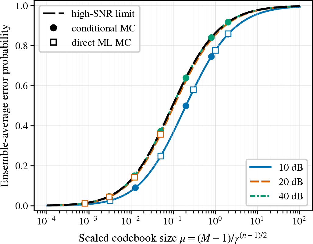
Figure 1 shows the ensemble-average error probability as a function of the scaled codebook size \[\mu=\frac{M-1}{\gamma^{(n-1)/2}}\] for \(n=6\). At 10 dB, a visible finite-SNR displacement from the limit \(F_n^{\mathrm{ens}}(\mu)\) remains. The 20- and 40-dB curves are progressively closer to \(F_n^{\mathrm{ens}}(\mu)\), and the 40-dB curve is nearly indistinguishable from the limiting curve \(F_n^{\mathrm{ens}}(\mu)\) over the displayed transition. The agreement occurs on the scaled-size axis rather than on the unnormalized codebook-size axis, confirming that \(M\asymp\gamma^{(n-1)/2}\) is the critical codebook-growth order.

The figure also displays both endpoints of the transition. For small \(\mu\), the error probability approaches zero, consistently with the underloaded regime in ?? ; for large \(\mu\), it approaches one, consistently with the overloaded regime in ?? . Between these endpoints, the nontrivial transition agrees with ?? . The conditional Monte Carlo and direct ML markers follow the corresponding finite-SNR curves throughout the accessible transition region.

7.3 Fixed-error rates↩︎

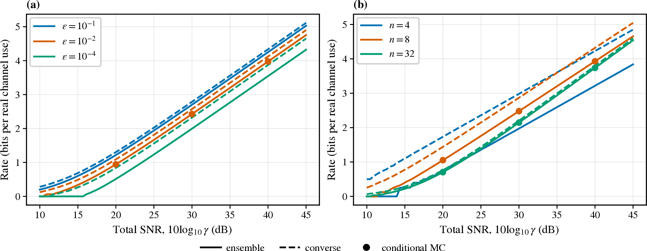
Figure 2 compares \(R_{\varepsilon,\mathrm{ens}}(n,\gamma)\) with \(R_{\varepsilon,\mathrm{conv}}(n,\gamma)\). In panel (a), the blocklength is fixed at \(n=16\) while the target error probability is varied. Increasing the reliability requirement lowers both rates through their constant high-SNR offsets, \(\mu_{n,\varepsilon}^{\mathrm{ens}}\) and \(\mu_{n,\varepsilon}^{\mathrm{conv}}\), while their leading slopes remain unchanged. This behavior is consistent with ?? and ?? : the target error probability enters the constant-order term but not the common prelog \((n-1)/(2n)\).

Panel (b) fixes \(\varepsilon=10^{-2}\) and varies the blocklength. The different high-SNR slopes reflect the blocklength-dependent prelog. Nevertheless, the rate is not ordered monotonically in \(n\) at a fixed total SNR. In particular, over the displayed range, \(n=32\) need not outperform \(n=8\), because the change in the constant rate offset can outweigh the prelog advantage. This observation is consistent with Proposition 5. In both panels the ensemble rate remains below the converse rate, as required by ?? , and the conditional Monte Carlo rate estimates agree with the ensemble curves.

The short zero-rate and curved portions at the lowest SNRs arise from the operational integer-codebook-size constraint. Once the admissible codebook size becomes large, the curves acquire their predicted high-SNR slopes.

7.4 Finite-SNR and limiting rate-bound gaps↩︎

To distinguish the finite-SNR rate difference from its limiting value, define \[\Delta_R(n,\varepsilon,\gamma) = R_{\varepsilon,\mathrm{conv}}(n,\gamma) - R_{\varepsilon,\mathrm{ens}}(n,\gamma). \label{eq:numerical-finite-snr-gap}\tag{56}\] Proposition 3 gives \[\Delta_R(n,\varepsilon,\gamma) = G(n,\varepsilon)+O_{n,\varepsilon}(\gamma^{-1/2}).\] Figure 3 compares \(\Delta_R(n,\varepsilon,\gamma)\) with the corresponding horizontal level \(G(n,\varepsilon)\).

Panel (a) fixes \(n=16\). More stringent reliability produces a larger limiting rate-bound gap, in agreement with the fixed-\(n\) reliability dependence in Theorem 4. Panel (b) fixes \(\varepsilon=10^{-2}\). The gap decreases markedly as the blocklength increases, consistently with the large-\(n\) expansion in 43 . In both panels, the finite-SNR differences approach their respective dotted limiting levels, and the conditional Monte Carlo points agree with the numerical rate differences.

The visible jumps and oscillations at the lowest SNRs, most prominently for \(\varepsilon=10^{-4}\) in panel (a) and \(n=4\) in panel (b), result from the integer thresholds defining the two finite-SNR rates. The difference of two quantized rate thresholds can change nonmonotonically when either admissible codebook size increases by one. Their magnitude rapidly becomes negligible as the codebook sizes grow.

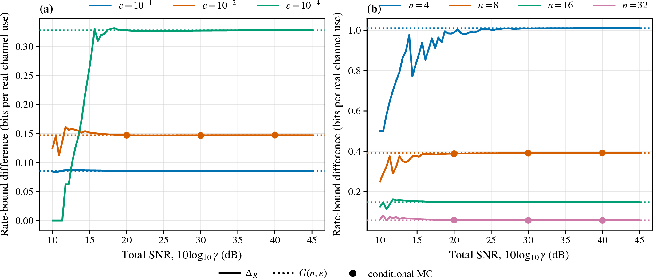
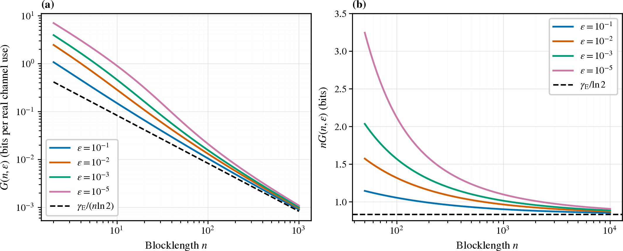
Figure 4 examines the dependence of the limiting gap on blocklength and reliability without a finite-SNR remainder. Panel (a) shows \(G(n,\varepsilon)\) over \(2\le n\le 10^3\). The log-log axes expose the leading \(1/n\) decay, and the curves approach the asymptotic law \(\gamma_{\mathrm E}/(n\ln2)\). At a fixed finite blocklength, a smaller target error probability produces a larger gap.

Panel (b) shows \(nG(n,\varepsilon)\) over \(50\le n\le10^4\). For every displayed fixed \(\varepsilon\), the curves approach the universal limit \(\gamma_{\mathrm E}/\ln2\) in 44 . The different approach rates are explained by the \(n^{-3/2}\) reliability-dependent term in 43 . Consequently, stringent reliability can delay the onset of the universal leading behavior even though it does not change the limit. These curves concern fixed \(\varepsilon\) as \(n\) increases; they do not represent the joint scaling \(\varepsilon=\varepsilon_n\) in 45 .

7.5 Rate-proxy-maximizing blocklength↩︎

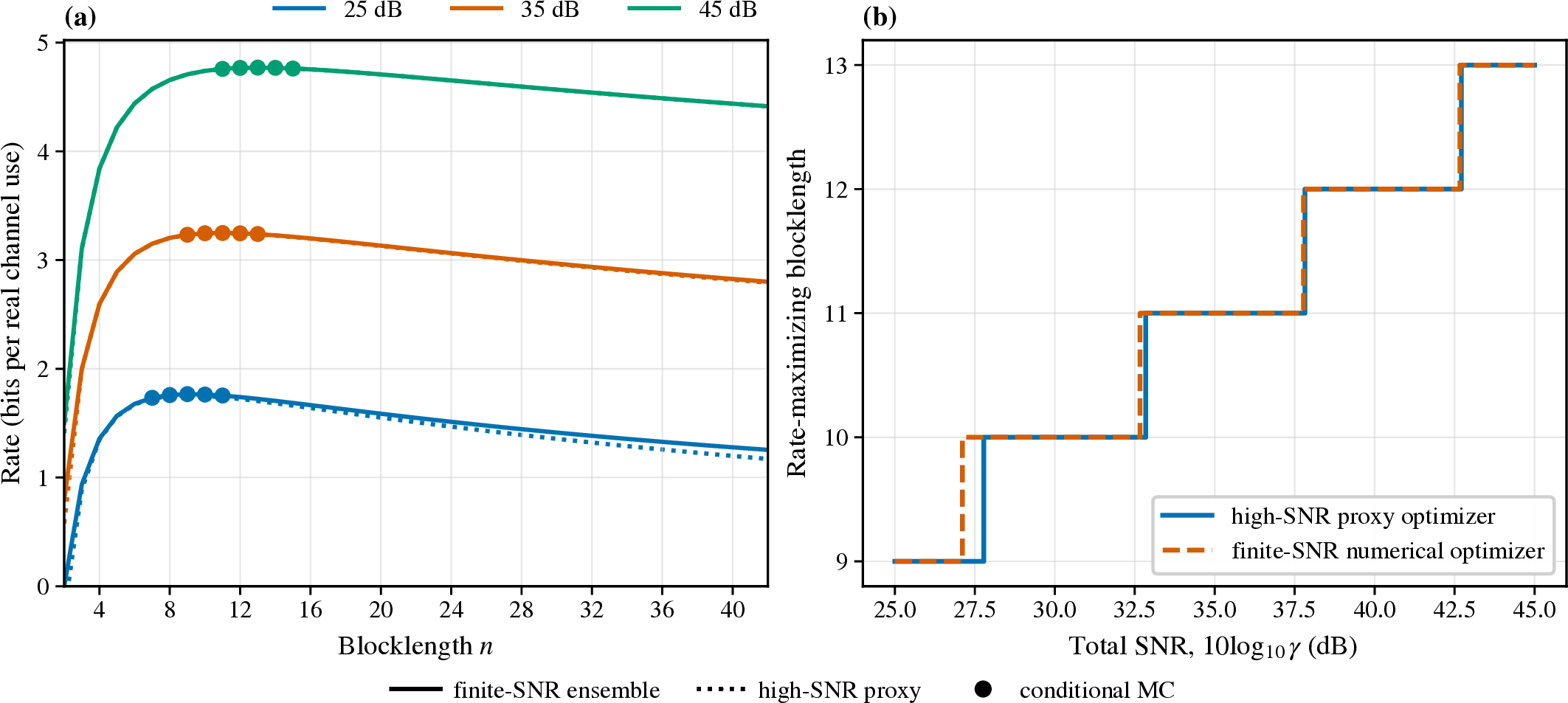
Figure 5 illustrates Proposition 5 for \(\varepsilon=10^{-2}\). Panel (a) compares the finite-SNR ensemble rate with the high-SNR proxy \(\widehat R_n(\gamma,\varepsilon)\) in 53 . At each displayed SNR, both curves initially increase with blocklength, attain interior maxima, and then decrease. Thus, at fixed total codeword-energy SNR and fixed target error probability, increasing the blocklength does not necessarily increase the finite-SNR rate.

As the SNR increases from 25 to 45 dB, both displayed maximizing blocklengths move from approximately \(n=9\) to \(n=13\), with maximizers near \(n=11\) at 35 dB. The high-SNR proxy closely follows the finite-SNR rate in a neighborhood of each maximum, and the conditional Monte Carlo points confirm the local rate behavior.

Panel (b) compares the smallest maximizer of the high-SNR proxy, \(\widehat n_R^\star(\gamma,\varepsilon)\), with the numerical maximizer of the finite-SNR ensemble rate over \(2\le n\le42\). The two staircase curves have nearly identical crossover locations, with the remaining small differences attributable to the finite-SNR remainder in 55 . The proxy optimizer is nondecreasing in SNR, as established in Proposition 5. This comparison is numerical over the displayed finite range and does not assert a uniform all-blocklength approximation.

8 Conclusion↩︎

This paper characterizes random spherical codebooks in the fixed-blocklength, high-SNR regime in which the codebook size grows with the total codeword-energy SNR. The critical growth order \(M(\gamma)\asymp\gamma^{(n-1)/2}\) separates underloaded, critically loaded, and overloaded error regimes. Inverting the critical transition gives the fixed-error data rate through its constant high-SNR term. Its prelog \((n-1)/(2n)\) agrees with that of the circular-cone converse for the equal-energy, average-error class, establishing first-order optimality of the ensemble-achievable rate; the relative rate shortfall decays as \(1/\ln\gamma\).

At fixed \((n,\varepsilon)\), the additive difference between the two rate bounds approaches the positive limiting gap \(G(n,\varepsilon)\). For fixed \(\varepsilon\), this gap satisfies \(G(n,\varepsilon)=\gamma_{\mathrm E}/(n\ln2) +O_\varepsilon(n^{-3/2})\) and therefore vanishes in the sequential high-SNR and large-blocklength limit. The joint analysis identifies the reliability exponent separating vanishing and nonvanishing gaps and quantifies the blocklength required for a prescribed gap. It also gives a pairwise crossover rule and a complete optimizer criterion for the fixed-\(n\) high-SNR rate proxy, showing why a larger blocklength need not give a larger rate proxy at fixed total SNR. The fixed-\(n\) rate expansion is not asserted to be uniform when \(n\) and \(\gamma\) grow simultaneously.

9 Scaled Dangerous-Cap Limit↩︎

This appendix proves Proposition 2.

Set \(\delta=\gamma^{-1/2}\), rotate coordinates so that the transmitted codeword is \(\mathbf{e}_1\), and couple all SNR values through the same noise vector. Write \[\mathbf{Z}=Z_\parallel\mathbf{e}_1+\mathbf{Z}_\perp, \qquad T_\perp=\frac{\|\mathbf{Z}_\perp\|^2}{2}, \qquad L_\delta=1+\delta Z_\parallel.\] Then \(T_\perp\sim\operatorname{Gamma}(a,1)\) and is independent of \(Z_\parallel\). By 16 , the exact dangerous-cap height is \[h_\delta = 1-\frac{L_\delta}{\sqrt{L_\delta^2+2\delta^2T_\perp}}.\] The beta representation gives \[I_{h/2}(a,a) = D_nh^a(1+O_n(h)), \qquad h\downarrow0. \label{eq:small-cap-prob-app}\tag{57}\] For the convergence rate, use the good event \[\mathcal{H}_\delta = \{|\delta Z_\parallel|\le1/2,\; \delta^2T_\perp\le1/2\}.\] On \(\mathcal{H}_\delta\), write \[S_\delta=\sqrt{L_\delta^2+2\delta^2T_\perp}.\] Then \[h_\delta=\delta^2T_\perp g_\delta, \qquad g_\delta=\frac{2}{S_\delta(S_\delta+L_\delta)}.\] Smoothness on the corresponding compact set and 57 imply \[\begin{align} &\left| \delta^{-2a}\Pi_\gamma-D_nT_\perp^a \right|\mathbf{1}_{\mathcal{H}_\delta} \\ &\quad\le C_nT_\perp^a \bigl(\delta|Z_\parallel|+\delta^2T_\perp\bigr) +C_n\delta^2T_\perp^{a+1}. \end{align}\] For \(q\in\{1,2\}\), the \(L^q\) norm of the right-hand side is \(O_{n,q}(\delta)\). On \(\mathcal{H}_\delta^c\), use \(0\le\Pi_\gamma\le1\) together with Gaussian and gamma Chernoff bounds; after multiplication by \(\delta^{-2a}\), the \(L^q\) contribution is \(o(\delta^b)\) for every fixed \(b>0\). Therefore, \[\left\| \gamma^a\Pi_\gamma-D_nT_\perp^a \right\|_q = O_{n,q}(\gamma^{-1/2}).\] Taking \(T=T_\perp\) proves ?? . For \(k\in\{1,2\}\), \[\mathbb{E}[\Theta_n^k] = D_n^k\frac{\Gamma((k+1)a)}{\Gamma(a)}.\] Taking expectations for \(k=1\) proves ?? ; the \(L^2\) convergence also gives \[\gamma^{2a}\mathbb{E}[\Pi_\gamma^2] \longrightarrow\mathbb{E}[\Theta_n^2],\] which is used in the Bonferroni estimate in Appendix 10.

10 Proofs of the Error Transition and Fixed-Error Data Rate↩︎

This appendix proves Theorem 1, Corollary 1, and Theorem 2. Put \(m=M-1\) and \(\mu=\mu(M,\gamma)=m/\gamma^a\).

10.1 Critical-scale approximation↩︎

For \(p\in[0,1]\) and every integer \(m\ge1\), the zero-count case of Le Cam’s inequality [11] gives \[0\le e^{-mp}-(1-p)^m\le2mp^2.\] The case \(m=0\) is immediate. Moreover, \(|e^{-x}-e^{-y}|\le|x-y|\) for \(x,y\ge0\). Since \(m=\mu\gamma^a\), the exact error representation gives \[\begin{align} &\left| \overline{P}_{\mathrm e}(M,n;\gamma)-F_n^{\mathrm{ens}}(\mu) \right| \\ &\quad\le 2m\mathbb{E}[\Pi_\gamma^2] + \mathbb{E}|m\Pi_\gamma-\mu\Theta_n| \\ &\quad= 2\mu\gamma^a\mathbb{E}[\Pi_\gamma^2] + \mu\mathbb{E}|\gamma^a\Pi_\gamma-\Theta_n|. \end{align}\] Proposition 2 and \(a\ge1/2\) show that the right-hand side is at most \(C_{n,K}\gamma^{-1/2}\), uniformly for \(0\le\mu\le K\). This proves ?? , and ?? follows immediately.

10.2 Underloaded and overloaded regimes↩︎

Suppose first that \(M(\gamma)\to\infty\) and \(\mu_\gamma\to0\). The first two Bonferroni inequalities applied to the competitor events give \[m\mathbb{E}[\Pi_\gamma] -\binom m2\mathbb{E}[\Pi_\gamma^2] \le\overline{P}_{\mathrm e}(M,n;\gamma) \le m\mathbb{E}[\Pi_\gamma].\] By ?? , \[m\mathbb{E}[\Pi_\gamma] =A_n\mu_\gamma \bigl(1+O_n(\gamma^{-1/2})\bigr),\] whereas the \(q=2\) part of Proposition 2 gives \[\binom m2\mathbb{E}[\Pi_\gamma^2] =O_n(\mu_\gamma^2).\] This proves ?? . The critical regime is the finite positive case of Theorem 1.

Now suppose \(\mu_\gamma\to\infty\). Put \(V_\gamma=\gamma^a\Pi_\gamma\). For any \(\zeta>0\), \[\begin{align} \mathbb{P}\{N_\gamma=0\} &=\mathbb{E}[(1-\Pi_\gamma)^m] \\ &\le \mathbb{P}\{V_\gamma\le\zeta\} +e^{-\zeta\mu_\gamma}. \end{align}\] Since \(V_\gamma\to\Theta_n\) in probability and \(\Theta_n>0\) almost surely, \[\limsup_{\gamma\to\infty}\mathbb{P}\{N_\gamma=0\} \le\mathbb{P}\{\Theta_n\le\zeta\}.\] Letting \(\zeta\downarrow0\) proves ?? and completes the proof of Corollary 1.

Finally, differentiation under the expectation gives \[\frac{\mathrm{d}}{\mathrm{d}\mu}F_n^{\mathrm{ens}}(\mu) = \mathbb{E}[\Theta_ne^{-\mu\Theta_n}]>0.\] Hence the curve is continuous and strictly increasing. Its endpoint values follow from dominated convergence and the fact that \(\Theta_n>0\) almost surely.

10.3 Fixed-error inversion↩︎

Let \(\mu_\varepsilon=\mu_{n,\varepsilon}^{\mathrm{ens}}\). Continuity of \(F_n^{\mathrm{ens}\,\prime}(\mu) =\mathbb{E}[\Theta_ne^{-\mu\Theta_n}]\) provides a neighborhood \(\mathcal{U}\) of \(\mu_\varepsilon\) and a constant \(c>0\) such that \(F_n^{\mathrm{ens}\,\prime}\ge c\) on \(\mathcal{U}\). Strict inequalities at the endpoints of \(\mathcal{U}\), together with ?? , place the threshold grid point \[\widehat\mu_\gamma =\frac{M_{\varepsilon,\mathrm{ens}}(n,\gamma)-1}{\gamma^a}\] and its successor in \(\mathcal{U}\) for all sufficiently large \(\gamma\). The threshold definition and the uniform error bound imply \[\begin{align} F_n^{\mathrm{ens}}(\widehat\mu_\gamma) &\le\varepsilon+C_{n,\varepsilon}\gamma^{-1/2},\\ F_n^{\mathrm{ens}}(\widehat\mu_\gamma+\gamma^{-a}) &>\varepsilon-C_{n,\varepsilon}\gamma^{-1/2}. \end{align}\] The mean-value theorem and \(\gamma^{-a}\le\gamma^{-1/2}\) therefore give \[\widehat\mu_\gamma=\mu_\varepsilon +O_{n,\varepsilon}(\gamma^{-1/2}),\] which is ?? . Taking \(n^{-1}\log_2(\cdot)\) gives ?? . Finally, if 27 holds, then \((M(\gamma)-1)/\gamma^a\to2^\eta\), and 28 follows from Theorem 1.

11 High-SNR Expansion of the Circular-Cone Converse↩︎

This appendix proves the high-SNR claims in Theorem 3. The underlying nonasymptotic converse is cited in the main text and is not rederived.

From 29 , \(\sin\phi=\phi(1+O(\phi^2))\) at the origin, and \(\int_0^\pi\sin^{n-2}\phi\,\mathrm{d}\phi =\sqrt\pi\,\Gamma((n-1)/2)/\Gamma(n/2)\), we obtain \[\Omega_n(\theta) =\kappa_n\theta^{n-1} \left[1+O_n(\theta^2)\right].\] This refines 30 to the error order needed below.

Uniformly whenever \(M/\gamma^a\) ranges over a fixed compact set \(K\subset(0,\infty)\), inversion of the same expansion and \(\tan\theta=\theta(1+O(\theta^2))\) give \[\sqrt\gamma\tan\theta_{n,M} =\left(\kappa_n\frac{M}{\gamma^a}\right)^{-1/(n-1)} \left[1+O_{n,K}(\gamma^{-1})\right]. \label{eq:uniform-cone-angle-expansion-app}\tag{58}\]

Suppose \(\mu(M_j,\gamma_j)\to\mu\in(0,\infty)\). Then 58 gives \(\sqrt{\gamma_j}\tan\theta_{n,M_j}\to (\kappa_n\mu)^{-1/(n-1)}\). Write \[\mathbf{Z}=Z_\parallel\mathbf{e}_1+\mathbf{Z}_\perp, \qquad \mathbf{Z}_\perp\in\mathbb{R}^{n-1}.\] On \(\{\sqrt{\gamma_j}+Z_\parallel>0\}\), whose complement has exponentially small probability, \[\begin{align} &\angle(\sqrt{\gamma_j}\mathbf{e}_1+\mathbf{Z},\mathbf{e}_1) >\theta_{n,M_j} \\ &\Longleftrightarrow\quad \|\mathbf{Z}_\perp\| >(\sqrt{\gamma_j}+Z_\parallel)\tan\theta_{n,M_j}. \end{align}\] The random threshold on the right therefore converges in probability to \((\kappa_n\mu)^{-1/(n-1)}\). Continuity of the \(\chi_{n-1}\) distribution proves ?? .

To compare the limiting curves, use \(D_n=2^a\kappa_n\) and define \[\tau_\mu=\frac{1}{2}(\kappa_n\mu)^{-1/a}.\] Since \(\mu D_n\tau_\mu^a=1\), both limiting curves can be expressed through \(T\sim\operatorname{Gamma}(a,1)\): \[\begin{align} F_n^{\mathrm{conv}}(\mu) &=\mathbb{P}\{T>\tau_\mu\}, \\ F_n^{\mathrm{ens}}(\mu) &=\mathbb{E}\left[1- \exp\left\{-\left(T/\tau_\mu\right)^a\right\}\right]. \end{align}\] Put \(X=(T/\tau_\mu)^a\). Its density is \[f_X(x)=\frac{\tau_\mu^a}{a\Gamma(a)} e^{-\tau_\mu x^{1/a}}, \qquad x>0,\] and is strictly decreasing. Hence \[\begin{align} &F_n^{\mathrm{ens}}(\mu)-F_n^{\mathrm{conv}}(\mu) \\ &\quad=\int_0^\infty \left(1-e^{-x}-\mathbf{1}\{x>1\}\right) f_X(x)\,\mathrm{d}x>0. \end{align}\] Indeed, the unweighted positive and negative parts have the same mass, \[\int_0^1(1-e^{-x})\,\mathrm{d}x =\int_1^\infty e^{-x}\,\mathrm{d}x=e^{-1},\] and strict decrease of \(f_X\) gives \[\int_0^1(1-e^{-x})f_X(x)\,\mathrm{d}x >f_X(1)e^{-1} >\int_1^\infty e^{-x}f_X(x)\,\mathrm{d}x.\] Both error probabilities are strictly between zero and one, which completes the proof of ?? .

To obtain the quantitative threshold, let \[\varphi_\gamma =\angle(\sqrt\gamma\mathbf{e}_1+\mathbf{Z},\mathbf{e}_1)\] and let \(\vartheta_{n,\varepsilon}(\gamma)\) be its unique upper \(\varepsilon\)-quantile. Put \(q_{n,\varepsilon}=\sqrt{s_{n-1,\varepsilon}}\). Uniformly for \(w\) in a compact subset of \((0,\infty)\), conditioning on \(Z_\parallel\) gives \[\begin{align} &\mathbb{P}\left\{\varphi_\gamma> \arctan\left(\frac{w}{\sqrt\gamma}\right)\right\} \nonumber\\ &\quad= \mathbb{E}\left[ Q_{n-1}\left(w^2(1+Z_\parallel/\sqrt\gamma)^2\right) \right]+O_n(e^{-\gamma/2}) \nonumber\\ &\quad=Q_{n-1}(w^2)+O_n(\gamma^{-1}). \label{eq:quantitative-cone-angle-app} \end{align}\tag{59}\] The linear Taylor term vanishes because \(\mathbb{E}[Z_\parallel]=0\); Gaussian tail truncation justifies the uniform second-order expansion. Since 58 keeps \(w\) in a compact subset of \((0,\infty)\), substituting \(w=\sqrt\gamma\tan\theta_{n,M}\) in 59 gives a uniform \(O_{n,K}(\gamma^{-1})\) approximation on every compact scaled-size interval \(K\subset(0,\infty)\). Since the \(\chi^2_{n-1}\) density is positive at \(s_{n-1,\varepsilon}\), quantile inversion yields \[\sqrt\gamma\tan\vartheta_{n,\varepsilon}(\gamma) =q_{n,\varepsilon}+O_{n,\varepsilon}(\gamma^{-1}). \label{eq:cone-quantile-rate-app}\tag{60}\] Furthermore, \[M_{\varepsilon,\mathrm{conv}}(n,\gamma) =\left\lfloor \Omega_n(\vartheta_{n,\varepsilon}(\gamma))^{-1} \right\rfloor.\] Combining 60 , the small-angle expansion, and the integer rounding error gives \[\begin{align} M_{\varepsilon,\mathrm{conv}}(n,\gamma) &=\mu_{n,\varepsilon}^{\mathrm{conv}}\gamma^a \left[1+O_{n,\varepsilon}(\gamma^{-1})\right]+O(1). \end{align}\] Taking logarithms, with the \(O(1)\) rounding term included, gives ?? . Finally, strict monotonicity of the two limiting curves and ?? give ?? .

12 Rate-Gap and Reliability–Blocklength Asymptotics↩︎

This appendix proves Proposition 3 and Theorem 4.

12.1 Exact gap identity↩︎

The constants in 20 and 30 satisfy \(D_n=2^a\kappa_n\). Since \(s_{n-1,\varepsilon}=2t_{a,\varepsilon}\), \[\mu_{n,\varepsilon}^{\mathrm{conv}} = \frac{1}{D_nt_{a,\varepsilon}^a}.\] Using \(r_{a,\varepsilon} =\mu_{n,\varepsilon}^{\mathrm{ens}}/ \mu_{n,\varepsilon}^{\mathrm{conv}}\) in \(F_n^{\mathrm{ens}} (\mu_{n,\varepsilon}^{\mathrm{ens}})=\varepsilon\) gives \[\mu_{n,\varepsilon}^{\mathrm{ens}}D_nT^a = r_{a,\varepsilon} (T/t_{a,\varepsilon})^a,\] which proves ?? . As \(r\) ranges from zero to infinity, its left-hand side is continuous and strictly increasing from zero to one, so the root is unique. Equivalently, ?? can be written as \[\mathcal{L}_a\!\left( \frac{r_{a,\varepsilon}}{t_{a,\varepsilon}^{a}} \right) =1-\varepsilon.\] Applying \(\mathcal{L}_a^{-1}\) proves ?? . Substitution into ?? proves ?? . The strict ordering ?? gives \(r_{a,\varepsilon}\in(0,1)\). Equations ?? and ?? follow from the two rate expansions. Dividing the latter identity by \(R_{\varepsilon,\mathrm{conv}}(n,\gamma)\) and using ?? proves ?? .

12.2 Fixed blocklength and increasing reliability↩︎

Fix \(a\) and write \(t=t_{a,\varepsilon}\). For \(X_t=(T/t)^a\), \[\mathbb{E}[X_t^k] = \frac{\Gamma((k+1)a)}{\Gamma(a)t^{ak}}, \qquad k\ge1.\] In particular, \[\frac{\mathbb{E}[X_t^2]}{\mathbb{E}[X_t]^2} =\frac{\Gamma(3a)\Gamma(a)}{\Gamma(2a)^2}<\infty.\] The upper and lower quadratic Taylor bounds for \(1-e^{-rX_t}\) and inversion at the origin therefore give \[r_{a,\varepsilon} = \varepsilon \frac{\Gamma(a)t_{a,\varepsilon}^a}{\Gamma(2a)} \left[1+O_a(\varepsilon)\right]. \label{eq:r-small-epsilon-app}\tag{61}\] The upper incomplete-gamma expansion gives \[\varepsilon = \frac{t^{a-1}e^{-t}}{\Gamma(a)} \left[1+O_a(t^{-1})\right], \qquad t\to\infty.\] With \(L=\ln(1/\varepsilon)\), inversion yields \[t_{a,\varepsilon} = L+(a-1)\ln L-\ln\Gamma(a) +O_a\left(\frac{\ln L}{L}\right). \label{eq:gamma-quantile-fixed-a-app}\tag{62}\] Substituting 62 into 61 and using \(G=-(n\ln2)^{-1}\ln r\) proves 41 . Replacing \(L\) by \(L+\ln10\) and subtracting proves 42 .

12.3 Fixed reliability and increasing blocklength↩︎

For fixed \(0<\varepsilon<1\), a Berry–Esseen bound for \(T\sim\operatorname{Gamma}(a,1)\), followed by quantile inversion, gives \[t_{a,\varepsilon} = a+z_\varepsilon\sqrt a+O_\varepsilon(1).\] Write \(s=\ln r\) and make the exact change of variables \(y=a\ln(T/t_{a,\varepsilon})\) in ?? . After subtracting the gamma-tail probability, the root equation becomes \[\int_{-\infty}^{\infty}d_s(y)w_a(y)\,\mathrm{d}y=0,\] where \[\begin{align} d_s(y) &=1-e^{-e^{s+y}}-\mathbf{1}\{y>0\}, \\ w_a(y) &= \frac{t_{a,\varepsilon}^a}{a\Gamma(a)} \exp\{y-t_{a,\varepsilon}e^{y/a}\}. \end{align}\] For every fixed \(C>0\), uniformly for \(s\) in a fixed compact set and \(|y|\le C\ln a\), \[\frac{w_a(y)}{w_a(0)} = 1-\frac{z_\varepsilon y}{\sqrt a} +O_\varepsilon\left(\frac{1+y^2}{a}\right).\] The required kernel integrals are \[\begin{align} \int_{-\infty}^{\infty}d_s(y)\,\mathrm{d}y &=s+\gamma_{\mathrm E}, \tag{63}\\ \int_{-\infty}^{\infty}y\,d_s(y)\,\mathrm{d}y &= -\frac{1}{2}(s+\gamma_{\mathrm E})^2-\frac{\pi^2}{12}. \tag{64} \end{align}\] These identities follow by viewing \(1-e^{-e^{s+y}}\) as the distribution function of \(\ln E-s\) for \(E\sim\operatorname{Exp}(1)\), whose mean and variance are \(-\gamma_{\mathrm E}-s\) and \(\pi^2/6\).

The kernel \(d_s(y)\) has integrable exponential tails, uniformly for \(s\) in compact sets. Dominated convergence first confines the root to a fixed compact interval around \(-\gamma_{\mathrm E}\); the central weight expansion can then be integrated term by term, with the tails controlled uniformly. Using 63 and 64 gives \[\begin{align} &\frac{1}{w_a(0)} \int_{-\infty}^{\infty}d_s(y)w_a(y)\,\mathrm{d}y \\ &\quad= s+\gamma_{\mathrm E} +\frac{z_\varepsilon}{\sqrt a} \left[ \frac{(s+\gamma_{\mathrm E})^2}{2} +\frac{\pi^2}{12} \right] +O_\varepsilon(a^{-1}), \end{align}\] uniformly on that interval. Root monotonicity now yields \[\ln r_{a,\varepsilon} = -\gamma_{\mathrm E} -\frac{\pi^2z_\varepsilon}{12\sqrt a} +O_\varepsilon(a^{-1}).\] Since \(n=2a+1\) and \(G=-(n\ln2)^{-1}\ln r\), this proves 43 and 44 .

12.4 Exponentially stringent reliability↩︎

Suppose 45 holds. The gamma large-deviation rate function is \[\mathcal{I}(q)=q-1-\ln q,\qquad q>0.\] Consequently, \[\frac{t_{a,\varepsilon_n}}{a}\longrightarrow q_\rho, \qquad \mathcal{I}(q_\rho)=2\rho.\]

For \(1<q_\rho<2\), make the change \(x=(T/t_{a,\varepsilon_n})^a\) in the root equation and normalize by the transformed density \(f_a\) at one. Its normalized ratio satisfies \[\frac{f_a(x)}{f_a(1)} =\exp\left\{-t_{a,\varepsilon_n} \bigl(x^{1/a}-1\bigr)\right\} \longrightarrow x^{-q_\rho}.\] Near zero, the root-equation kernel is \(O(x)\), which is integrable against \(x^{-q_\rho}\) precisely when \(q_\rho<2\); at infinity it decays exponentially for \(r\) in a compact neighborhood of the positive limiting root. Dominated convergence therefore yields \[\begin{align} 0 &= \int_0^\infty \left( 1-e^{-rx}-\mathbf{1}\{x>1\} \right)x^{-q_\rho}\,\mathrm{d}x \\ &= \frac{ \Gamma(2-q_\rho)r^{q_\rho-1}-1 }{q_\rho-1}. \end{align}\] Monotonicity of the finite-\(a\) and limiting roots therefore gives \[r_{a,\varepsilon_n} \longrightarrow \Gamma(2-q_\rho)^{-1/(q_\rho-1)}.\] In particular, \(G(n,\varepsilon_n)\to0\).

For \(q_\rho\ge2\), use \[(1-e^{-1})\min\{u,1\} \le1-e^{-u}\le\min\{u,1\}, \qquad u\ge0.\] Define \[J_a(r) =\mathbb{E}\left[\min\left\{1,r(T/t_{a,\varepsilon_n})^a\right\}\right].\] For a fixed trial \(r=e^{-a\sigma}\) with \(\sigma\ge0\), truncate \(T/a\) to a compact interval, apply the gamma large-deviation principle there, and then remove the truncation by exponential tightness. This gives \[\begin{align} -\frac{1}{a}\ln J_a(e^{-a\sigma}) &\longrightarrow K_q(\sigma), \nonumber\\ K_q(\sigma) &= \min\left\{ 1+\sigma+\ln q-2\ln2,\, \mathcal{I}(qe^\sigma) \right\}, \label{eq:supercritical-Laplace-app} \end{align}\tag{65}\] where \(q=q_\rho\). With \((x)_+=\max\{x,0\}\), the variational form is \[K_q(\sigma) =\inf_{u>0} \left\{\mathcal{I}(u)+\bigl(\sigma-\ln(u/q)\bigr)_+\right\}.\] Splitting the infimum at \(u=qe^\sigma\) gives the two branches in 65 : the unsaturated branch is minimized at \(u=2\), whereas the saturated branch is minimized at its left endpoint. The unique solution of \(K_q(\sigma)=\mathcal{I}(q)\) is zero when \(q=2\) and \[\sigma=q-2-2\ln(q/2)\] when \(q>2\). At the exact root, the constant-factor bounds above imply \(-a^{-1}\ln J_a(r_{a,\varepsilon_n})\to \mathcal{I}(q)\). When \(q>2\), the solution is positive. Applying the Laplace limit at fixed trial values on either side of this solution and using monotonicity brackets \(-a^{-1}\ln r_{a,\varepsilon_n}\) around the solution.

At the boundary \(q=2\), the argument is one-sided because the solution \(\sigma=0\) lies at the edge of the domain \(\sigma\ge0\). The ordering \(r_{a,\varepsilon_n}<1\) gives \(-a^{-1}\ln r_{a,\varepsilon_n}\ge0\). For every \(\delta>0\), \(K_2(\delta)>\mathcal{I}(2)\), so the constant-factor bounds and the Laplace limit show that the root-equation left-hand side at the trial value \(r=e^{-a\delta}\) is eventually smaller than \(\varepsilon_n\). Monotonicity then gives \(r_{a,\varepsilon_n}>e^{-a\delta}\) and hence \(\limsup[-a^{-1}\ln r_{a,\varepsilon_n}]\le\delta\). Letting \(\delta\downarrow0\) proves the boundary case. Thus \[-\frac{1}{a}\ln r_{a,\varepsilon_n} \longrightarrow q_\rho-2-2\ln(q_\rho/2), \qquad q_\rho\ge2.\] Division by \(n\ln2\) proves 47 for \(q_\rho>2\) and gives \(G(n,\varepsilon_n)\to0\) at \(q_\rho=2\). This boundary corresponds to \(\rho_{\mathrm c}=(1-\ln2)/2\), proving 48 .

13 Proofs of the Blocklength Design Results↩︎

This appendix proves Propositions 4 and 5.

13.1 Blocklength inversions↩︎

For fixed \(\varepsilon\), substitute \[n=N_0(G_0) +\frac{c_0z_\varepsilon}{\gamma_{\mathrm E}} \sqrt{N_0(G_0)}+x\] into 43 . Taking \(x\) to be fixed and positive or fixed and negative gives a two-sided localization. More explicitly, the \(O_\varepsilon(n^{-2})\) remainder is uniform for \(n\) in a fixed relative neighborhood of \(N_0(G_0)\). Hence a sufficiently large constant \(K_\varepsilon\) satisfies the following, where \(b_\varepsilon(G_0)\) denotes the displayed center: \[\begin{align} n\le b_\varepsilon(G_0)-K_\varepsilon &\quad\Longrightarrow\quad G(n,\varepsilon)>G_0,\\ n\ge b_\varepsilon(G_0)+K_\varepsilon &\quad\Longrightarrow\quad G(n,\varepsilon)<G_0, \end{align}\] for all sufficiently small \(G_0\), within that neighborhood. The leading \(1/n\) term excludes smaller growing blocklengths, while every fixed finite collection of blocklengths has a positive minimum gap and is also excluded as \(G_0\downarrow0\). Thus the smallest qualifying integer lies within \(O_\varepsilon(1)\) of the displayed center. This proves 50 ; subtracting the expansions at \(\varepsilon\) and \(\varepsilon/10\) gives 51 .

For the ultra-reliable inversion, define \[\mathfrak G(\rho) = \begin{cases} 0, &0\le\rho\le\rho_{\mathrm c},\\[2pt] \dfrac{ q_\rho-2-2\ln(q_\rho/2) }{2\ln2}, &\rho>\rho_{\mathrm c}. \end{cases}\] This function is continuous and strictly increasing above \(\rho_{\mathrm c}\), and \(\mathfrak G(\rho_{G_0})=G_0\). Put \(L=\ln(1/\varepsilon)\) and fix \(0<\delta<\rho_{G_0}\). The trial blocklength \[n_+(\varepsilon) =\left\lceil\frac{L}{\rho_{G_0}-\delta}\right\rceil\] satisfies \(L/n_+(\varepsilon)\to\rho_{G_0}-\delta\) and is therefore feasible for all sufficiently small \(\varepsilon\). Thus \(n_G(\varepsilon,G_0)\le n_+(\varepsilon)\) eventually.

For the matching lower bound, every integer \[n\le \left\lfloor\frac{L}{\rho_{G_0}+\delta}\right\rfloor\] is eventually infeasible. Otherwise, there would be a sequence \(\varepsilon_k\downarrow0\) and feasible \(n_k\) in this range. After passing to a subsequence, one of three cases must hold: \(n_k\) is bounded; \(n_k\to\infty\) and \(L_k/n_k\) has a finite limit at least \(\rho_{G_0}+\delta\); or \(L_k/n_k\to\infty\), where \(L_k=\ln(1/\varepsilon_k)\). The first case is excluded by 41 ; the second is excluded by Theorem 4 and the strict increase of \(\mathfrak G\) above \(\rho_{\mathrm c}\). It remains to exclude the third case.

For a sequence in the third case, define locally in this proof \[U_n=\frac{\Gamma(a)}{\Gamma(2a)}T^a, \qquad \mathbb{E}[U_n]=1,\] and let \(\lambda_{n,\varepsilon}\) solve \(\mathbb{E}[1-e^{-\lambda_{n,\varepsilon}U_n}]=\varepsilon\). Then \[r_{a,\varepsilon} = \lambda_{n,\varepsilon} \frac{\Gamma(a)t_{a,\varepsilon}^a}{\Gamma(2a)}.\] Moreover, \[\mathbb{E}[U_n^2] = \frac{\Gamma(3a)\Gamma(a)}{\Gamma(2a)^2} = \exp\{a\ln(27/16)+O(\ln a)\}.\] If \(L_n=\ln(1/\varepsilon_n)\) and \(L_n/n\to\infty\), the Taylor bounds for \(1-e^{-x}\) can be applied quantitatively. Indeed, \(\varepsilon_n\mathbb{E}[U_n^2]\to0\) because \(L_n/a\to\infty\); evaluating the lower Taylor bound at \(2\varepsilon_n\) and using \(\mathbb{E}[U_n]=1\) gives \[\varepsilon_n \le\lambda_{n,\varepsilon_n} \le2\varepsilon_n\] along every unbounded-blocklength subsequence. A gamma-tail Chernoff bound also gives \[\ln\frac{t_{a,\varepsilon_n}}{a} =O\left( \ln\left(1+\frac{L_n}{a}\right) \right).\] Together with Stirling’s formula and \(L_n/a\to\infty\), this yields \[\ln\left[ \frac{\Gamma(a)t_{a,\varepsilon_n}^a}{\Gamma(2a)} \right] =o(L_n).\] Consequently, \(-\ln r_{a,\varepsilon_n}\sim L_n\) and \(G(n,\varepsilon_n)\to\infty\), which is the required contradiction. We have therefore bounded \(n_G(\varepsilon,G_0)\) between \(L/(\rho_{G_0}+\delta)+O(1)\) and \(L/(\rho_{G_0}-\delta)+O(1)\). Divide by \(L\) and let \(\delta\downarrow0\) to prove 52 .

13.2 Maximization of the high-SNR rate proxy↩︎

Stirling’s formula, the fixed-\(\varepsilon\) gamma-quantile expansion, and the large-\(n\) behavior of \(r_{a,\varepsilon}\) give \(\ln\mu_n=-\tfrac12(n-1)\ln(n-1)+O_\varepsilon(n)\). Thus \(\widehat R_n(\gamma,\varepsilon)\to-\infty\) as \(n\to\infty\) for fixed \(\gamma\), so the maximum in Proposition 5 is attained. Subtracting the two expressions in 53 and using 54 gives ?? . Hence the proxy at a candidate \(n\) is at least as large as the proxy at every smaller blocklength precisely when \(\gamma\ge\gamma_n^-(\varepsilon)\), and it is at least as large as the proxy at every larger blocklength precisely when \(\gamma\le\gamma_n^+(\varepsilon)\). This proves ?? and ?? . Finally, the slope \((n-1)/(2n)\) in 53 is strictly increasing in \(n\), so the smallest proxy maximizer cannot decrease as \(\gamma\) increases.

References↩︎

---

1. N. Zlatanov is with Innopolis University, Innopolis, 420500, Russia (e-mail: n.zlatanov@innopolis.ru).↩︎