Clean-Reference Streaming Detection of Lens Occlusion and Photometric Transitions for Camera Tamper Monitoring
July 16, 2026
Abstract
A surveillance camera is an image sensor whose silent physical degradation invalidates every downstream consumer of its data. In-situ integrity alarms for such vision sensors require low false-alarm rates, bounded computation, and diagnosable behavior under nuisance illumination changes. This paper studies a deliberately narrow streaming integrity monitor for two low-cost sensor-fault signatures: texture-collapsing lens occlusion and abrupt photometric scene transition. The detector compares sampled luminance and local-gradient statistics with a clean-only sliding reference, applies coarse-grid structured-light rejection and mode/rapid-brightness suppression, and emits at most one notification per tamper episode. We formalize the decision predicates and derive a consistency rule for when rapid-brightness suppression makes the scene-transition path unreachable. On 320 in-scope controlled sequences, the default state machine attains 0.800 F1 and 0.822 balanced accuracy (significantly better paired correctness than the strongest baseline, though the F1 margin is not statistically resolved); on a magnitude-swept public audit it attains the highest partial AUC under a 5% false-alarm budget, and a separate extended-stress FPR-constrained sweep reaches 0.925 recall at 0.025 false-positive rate. Public Xiph, Bremen IoT, and UHCTD diagnostics show the fixed predicates preserve low false alarms while recall concentrates inside the declared envelope (UHCTD in-scope covered recall 0.667 versus 0.016 out of scope), and a 9.09-camera-hour verified-negative public audit records zero false alarms. The method is best interpreted as an auditable sensor-health subsystem rather than a universal camera-tamper classifier.
Camera health monitoring, false-alarm control, image sensors, lens occlusion, photometric scene transition, sensor fault detection, streaming detection, video surveillance.
1 Introduction↩︎
A surveillance camera is, above all, an image sensor, and physical interference with that sensor — covering the lens, changing its focus, moving the camera — silently invalidates all analytics downstream of image acquisition, while day–night switching, exposure control, room-light toggles, and large foreground objects produce equally abrupt image changes. This is a sensor-reliability problem: a single camera-health signal gates the availability and trustworthiness of every downstream consumer of the sensor’s data, so a useful in-situ integrity monitor must balance response latency, nuisance rejection, predictable computational cost, and diagnosable behavior. Throughout the paper, tamper names the physical event class, while sensor-integrity or camera-health names the system-facing signal that reports it.
Prior systems compare current frames with buffered references using histograms, edges, frequency coefficients, keypoints, or learned representations [1]–[4]. The present work addresses a narrower engineering point: how low-cost photometric and texture cues can be composed into a stateful decision rule whose baseline cannot absorb an active alarm and whose suppression logic is auditable. The novelty is this stateful, auditable composition rather than the individual scalar cues: an active alarm cannot update the clean reference, nuisance transitions are handled by explicit negative gates, and the emission policy is episode-based rather than per-frame — a trade that matters in embedded pipelines where deterministic behavior, bounded state, and failure diagnosis outweigh an opaque classifier.
The method is deliberately not presented as a universal covered–defocused–moved camera classifier. Its positive scope comprises (i) lens obstruction producing a sufficiently large texture collapse with a bounded luminance change and (ii) a scene transition producing a sufficiently large luminance change; pure rotation or translation that preserves global statistics, subtle local occlusion, defocus without the required mean shift, and video-file forgery all fall outside that positive guarantee.
The contributions are:
a clean-reference streaming state machine for two declared vision-sensor fault signatures: texture-collapsing lens occlusion and abrupt photometric scene transition;
an implementation-faithful formulation of the mean, gradient, grid, suppression, and episode predicates, with diagnostic metadata for field triage;
a configuration-safety condition showing when rapid-brightness suppression makes the scene-transition path unreachable;
a false-alarm-constrained evaluation protocol with paired baselines, targeted ablations, and public-data diagnostics; and
a deployment boundary showing where fixed photometric predicates end and registration, calibration, or learned references begin.
2 Related Work↩︎
2.1 Reference-Based and Hand-Crafted Detectors↩︎
Ribnick et al. compared buffered old and recent frames using normalized distance measures [1]; Saglam and Temizel developed adaptive detectors for obstruction, displacement, and focus changes emphasizing low false-alarm operation [2]; Tung et al. classified tamper events over an adaptive background codebook [5]; and Roy et al. proposed a robust background-model update that resists a slowly corrupted reference [6]. These methods establish the value of a temporal reference but also expose reference contamination and threshold calibration as practical concerns. Edge loss is a particularly common cue because cover and defocus remove high-frequency content: Lee et al. measured edge disappearance relative to a background image with foreground-object exclusion [3], Shi et al. combined background construction with local-binary-pattern similarity [7], and Sitara and Mehtre added foreground coverage area and its temporal stability [8].
2.2 Camera Displacement and Registration-Based Detection↩︎
Because global mean and sampled gradient are largely insensitive to a rigid viewpoint change, several prior systems add an explicit geometric cue, from SIFT keypoint-geometry verification [9] to the registration and motion-compensation strategies surveyed by Chapel and Bouwmans [10]. We do not implement a registration baseline in this paper; Section 5.7 instead measures, on real camera-disjoint images, how far a purely photometric predicate is from covering this case on its own.
2.3 Statistical, Learned, and Calibrated References↩︎
Mantini and Shah modeled normal signal activity with a Gaussian mixture and temporal filtering [4], later learned a generative reference with deep feature comparison [11], released the UHCTD dataset with deep-classifier benchmarks on covered/defocused/moved/normal frames — the closest prior work to a learned camera-tamper baseline [12] — and surveyed which hand-crafted feature families transfer best across cameras [13]. Pan detected physical camera-integrity attacks with a deep video-frame-interpolation anomaly score [14]. Such learned models represent broader appearance variation but introduce training data, model storage, and domain-transfer requirements; Sidnev et al. highlighted the difficulty of per-camera threshold selection even for low-level features [15]. More broadly, camera tamper detection is one instance of video anomaly detection [16], and false-alarm-constrained evaluation is standard in adjacent visual-inspection settings [17]; our evaluation adopts the same convention.
Our approach occupies a different point in this design space: no pixelwise background modeling or foreground masks [3], no trained probabilistic or deep reference [4], [11], [12], no automatic calibration claim [15], and no geometric registration cue [9], [10]. The distinctive element is the composition of sampled statistics, clean-only reference maintenance, structural nuisance rejection, and explicit operational state; the intended advantages are simplicity, auditability, and bounded state, with geometric invariance and cross-camera tuning delegated to complementary modules.
2.4 Embedded Analytics and Sensor Self-Validation↩︎
Hand-crafted cues remain relevant when throughput and resource bounds dominate, as in FPGA [18], DSP [19], low-power smart-camera [20], and single-board-computer [21] tamper detectors; this body of work motivates our emphasis on bounded, auditable arithmetic evaluated as a hardware-agnostic algorithmic contribution. Camera tampering is also an instance of the broader sensor-fault-detection problem: self-validating sensor concepts attach an online validity status and diagnostics to every measurement [22], surveys and classifiers for outlier and fault detection in wireless-sensor and IoT deployments organize the corresponding principles for low-cost distributed sensors [23]–[25], and automotive perception likewise treats camera degradation as a sensor-level reliability concern [26]. The present detector follows the same design logic at the level of an image sensor — validate the stream in situ with bounded arithmetic, attach diagnostic metadata to every alarm, and expose a health signal that gates downstream analytics — motivating auditability and false-alarm control over maximal classification power.
3 Problem Scope and Output Semantics↩︎
Let \(I_t\in[0,255]^{H\times W}\) be a grayscale frame acquired at timestamp \(\tau_t\). The detector emits \(\mathbf{y}_t=(d_t,c_t,z_t,m_t)\), where \(d_t\in\{0,1\}\) is an alarm, \(c_t\in[0,1]\) is a cue magnitude rather than a calibrated posterior probability, \(m_t\) is diagnostic metadata, and \(z_t\in\{\mathrm{no\;tamper},\) \(\mathrm{occlusion\;event},\) \(\mathrm{scene\;transition}\}\). The second label denotes an abrupt photometric scene transition. It should not be read as a registration-based guarantee for every camera displacement.
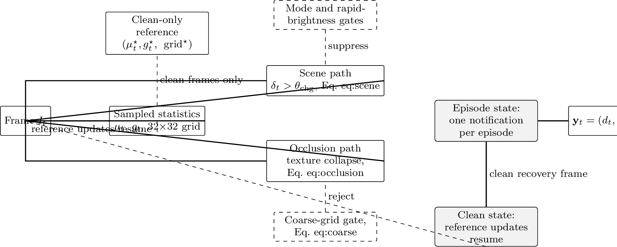
The detector holds a window of at most \(N\) frames accepted as clean. Its scalar reference is \((\mu_t^\star,g_t^\star)\), and its structural reference is a per-cell mean on a \(32\times32\) grid. Frames declared tampered are never inserted into these references. The declared operating envelope is: in scope — a texture-collapsing cover with a bounded mean shift, and an abrupt photometric scene transition not suppressed by the mode or rapid-brightness gates; out of scope or weak — pure camera rotation or translation (global statistics carry no registration evidence), mean-preserving defocus, and subtle local partial covers; intended nuisance rejection — global illumination steps; ambiguous, requiring field validation — foreground objects close to the lens; and excluded from accuracy metrics — unreadable or failed clips (each condition is tabulated with its mechanistic reason in the supplementary material).
3.1 Clip-Level Ground Truth for Evaluation↩︎
The per-frame alarm \(d_t\) is a prediction. Evaluating that prediction requires a separate, independently defined ground-truth label, and the two must not be conflated. We define them as follows.
A clip is ground-truth positive if and only if at least one declared in-scope condition genuinely occurred at some point during the entire recording, independent of whether the detector raised an alarm, and ground-truth negative only if no such condition occurred anywhere in the full recording. This is a claim about the physical recording session, not a sampled subset of its frames; a brief or previously unnoticed occurrence anywhere in the clip makes it positive.
Consequently, “the detector did not alarm” is not evidence that a clip is ground-truth-negative: a predicted-negative clip with a missed genuine event is a false negative, and a true negative requires independent confirmation — exhaustive review of the full recording or an authoritative collection record, not a coarse pass over sampled frames or the absence of a reported incident. This definition governs every true-negative, false-negative, specificity, and false-positive-rate statement in the paper; where labels do not meet it, we report a conservative accounting convention instead of a true-negative count.
4 Streaming Tamper Detector↩︎
4.1 Sampled Photometric and Texture Statistics↩︎
Let \(x\) index columns and \(y\) index rows throughout, so \(x\equiv0\pmod 4\) selects every fourth column. Mean extraction visits every row and every fourth column: \[\begin{align} \Omega_\mu=\{(x,y):&\;0\le x<W,\;0\le y<H,\\ & x\equiv0\pmod 4\}. \end{align}\] The sampled mean is \[\mu_t=\frac{1}{|\Omega_\mu|}\sum_{(x,y)\in\Omega_\mu} I_t(x,y).\] The local-gradient proxy samples both axes every four pixels but compares immediate neighbors: \[\begin{align} \Omega_g=\{(x,y):&\;0\le x<W-1,\;0\le y<H-1,\\ & x\equiv0\pmod 4,\;y\equiv0\pmod 4\}. \end{align}\] \[g_t=\frac{1}{2|\Omega_g|}\sum_{(x,y)\in\Omega_g} \left(d^x_t(x,y)+d^y_t(x,y)\right),\] where \(d^x_t=|I_t(x+1,y)-I_t(x,y)|\) and \(d^y_t=|I_t(x,y+1)-I_t(x,y)|\). Immediate differences avoid aliasing a one-pixel texture into an apparently flat image; border pixels lacking a right or lower neighbor are excluded.
During warm-up, a frame is treated as boot-time occlusion if \[\mu_t<\theta_{\mathrm{boot,dark}}\;\lor\; g_t<\theta_{\mathrm{boot,flat}},\] with implementation defaults \(\theta_{\mathrm{boot,dark}}=15\) intensity levels and \(\theta_{\mathrm{boot,flat}}=2\) gradient levels (the controlled evaluation of Section V disables the flatness check). Such frames are emitted but excluded from warm-up. Recovery clears the partially collected reference before accepting new clean frames. Once \(N\) clean frames are available, running sums give constant-time reference updates: \[\mu_t^\star=\frac{1}{N}\sum_{k\in\mathcal{W}_t}\mu_k, \qquad g_t^\star=\frac{1}{N}\sum_{k\in\mathcal{W}_t}g_k.\]
4.2 Photometric Scene-Transition Path↩︎
Define the inter-frame mean jump \(\delta_t=|\mu_t-\mu_{t-1}|\), current and previous texture-collapse indicators \[o_t=\mathbb{I}[g_t<\theta_{\mathrm{occ}}g_t^\star],\qquad o_{t-1}=\mathbb{I}[g_{t-1}<\theta_{\mathrm{occ}}g_t^\star],\] where both frames are deliberately tested against the current reference \(g_t^\star\): the clean window is frozen while a candidate is active, so \(g_t^\star\) is the most recent uncontaminated texture reference for either frame, and normalized gradient change \[q_t=\frac{g_{t-1}-g_t}{\max(g_t^\star,\epsilon)}.\] The primary scene candidate is \[\mathcal{C}^{\mathrm{sc}}_t= [\delta_t>\theta_{\mathrm{chg}}]\land[\neg o_t\lor o_{t-1}] \land[\rho_{\mathrm{grad}}\le0\lor q_t\ge\rho_{\mathrm{grad}}]. \label{eq:scene}\tag{1}\] A counter requires \(K\) consecutive candidates when persistence is enabled. A secondary luminance route compares the current mean with both the last accepted clean mean and the sliding mean, requiring an absolute jump above \(\theta_{\mathrm{chg}}\) and a relative jump above the auxiliary ratio \(\rho_{\mathrm{lumin}}\) (default 0.8); in the evaluated pathway it adds baseline-relative luminance memory only.
4.3 Gradient-Collapse Occlusion Path↩︎
If the scene path has not fired, an occlusion candidate requires the conjunction \[\begin{align} g_t &<\theta_{\mathrm{occ}}g_t^\star,\\ \Delta_{\min}<|\mu_t-\mu_t^\star|&\le\Delta_{\max},\\ \mu_{\min}\le\mu_t&\le\mu_{\max}, \end{align} \label{eq:occlusion}\tag{2}\] so that Eq. 2 denotes all three conditions jointly. The lower bound is \(\Delta_{\min}=20\) intensity levels in the implementation; the upper bound and absolute luminance interval reject extreme environmental transitions. Consequently, defocus that reduces texture without also satisfying the mean constraint is not guaranteed to trigger.
For each frame, a \(32\times32\) center-sampled luminance grid is compared with its clean reference. Let \(r_{20}\) be the fraction of cells changing by more than 20, \(\bar\sigma_b\) the mean standard deviation over \(4\times4\) grid blocks, and \(r_{\mathrm{flat}}\) the fraction of blocks with standard deviation below 3. A low-gradient candidate is rejected as structured lighting change when \[\begin{align} &(r_{20}>0.85\land\bar\sigma_b>10\land r_{\mathrm{flat}}<0.25)\nonumber\\ &\quad\lor(\bar\sigma_b>18\land r_{\mathrm{flat}}<0.20 \land g_t/g_t^\star>0.40). \label{eq:coarse} \end{align}\tag{3}\] The grid is thus a negative gate for occlusion, not a third positive detector.
4.4 Transition Suppression and Configuration Consistency↩︎
A change in the externally supplied day–night flag (the operating-mode gate, hereafter the mode gate) suppresses scene output for that transition; on typical cameras this flag derives from the IR-cut-filter state or the sensor front end’s exposure/gain metadata. Separately, if \(\delta_t>\theta_{\mathrm{rapid}}\), the timestamp is stored and scene output is suppressed for \(T_{\mathrm{sup}}\). These gates do not suppress an occlusion that independently satisfies 2 .
The two brightness thresholds cannot be tuned independently. If \(T_{\mathrm{sup}}>0\) and \(\theta_{\mathrm{rapid}}\le\theta_{\mathrm{chg}}\), every frame satisfying \(\delta_t>\theta_{\mathrm{chg}}\) also starts the rapid-brightness window before the scene decision. The primary scene path is therefore unreachable on that frame. We impose the consistency rule \[T_{\mathrm{sup}}=0\quad\lor\quad \theta_{\mathrm{rapid}}>\theta_{\mathrm{chg}}. \label{eq:consistency}\tag{4}\] Persistence \(K>1\) confirms a multi-frame transition, not a single step followed by a stable new view.
4.5 Episode State, Complexity, and Invariants↩︎
Two binary episode states select per-frame or once-per-episode emission; a clean decision ends the episode and updates all clean references, and scene decisions precede primary occlusion decisions. Mean extraction costs \(\mathcal{O}(HW/4)\), gradient extraction \(\mathcal{O}(HW/16)\), and the fixed grid \(\mathcal{O}(32^2)\); storage is \(\mathcal{O}(N)\) scalars plus \(\mathcal{O}(N\cdot32^2)\) bytes. Three invariants make the detector auditable in a larger pipeline: reference safety (no alarming frame is ever inserted into the scalar or grid reference, so a sustained occlusion cannot be absorbed by the baseline), episode non-duplication (later positive frames belong to the active episode until a clean recovery frame resets it), and scene-path reachability (the consistency rule of Eq. 4 ).
5 Controlled Evaluation↩︎
Table 1 maps every evaluation protocol in this paper to its data source, unit of analysis, and the question it answers; the same method row can therefore appear under different scopes without those scopes being comparable.
| Protocol | Data | Units | Question |
|---|---|---|---|
| Controlled stress (Table [tbl:tab:controlled]) | 8 background videos, fixed synthetic magnitudes | 400 seq. | primary in-scope comparison |
| Sensitivity grid (suppl.) | same | 400 seq. | parameter sensitivity |
| Extended stress, probes (suppl.) | synthetic gate stressors | 30–60 seq.each | per-gate behavior |
| Xiph audits | public videos | frames / seq. | reproducibility, latency |
| Magnitude sweep (Fig. [fig:magnitude95detectability]) | public videos, swept magnitudes | 250 seq. | decoupled operating characteristics |
| IoT cross-check (suppl.) | public stills, 2 cameras | images | untuned cross-camera transfer |
| UHCTD diagnostic (suppl.) | public video, 2 cameras | 4.5M frames | real-video boundary, in-scope stratification |
| Long-negative audit (suppl.) | VIRAT + CDnet2014 negatives | 9.09 cam.-h | verified-negative false alarms |
2.6pt
5.1 Protocol and Baselines↩︎
Ten random 48-frame clips are drawn from each of eight background videos (every third source frame, resized to \(160\times90\)), and five deterministic conditions are generated per clip, yielding 400 labeled sequences: clean, texture-collapsing cover, photometric scene replacement, geometry-preserving rotation/translation, and a global illumination step. Cover and photometric replacement are the declared in-scope positives; clean and illumination-step sequences are negatives; the geometric shift is an out-of-scope diagnostic that tests the absence of registration evidence. Perturbations begin at frame 16, after a 12-frame reference window; the seed is fixed to 20260701.
We compare six methods on identical sequences. The five baselines are transparent, deployable without training, and representative of the mean, gradient, edge, frame-difference, and histogram cues used in lightweight tamper detection: mean jump (any post-onset \(|\mu_t-\mu_{t-1}|>80\)), gradient collapse (\(g_t<0.45g^\star\) after warm-up), an edge-reference proxy (a literature-motivated Sobel edge-disappearance baseline without object masks, not claimed as an exact reproduction of [3]), frame difference (mean absolute difference from the clean reference frame above 35 levels), and histogram difference (Bhattacharyya distance from the clean reference histogram above 0.35). Complete published detectors such as Saglam and Temizel’s adaptive scheme [2] depend on pixelwise background maintenance outside the bounded-state family studied here and are represented by their constituent cues. The full state machine runs Eqs. 1 –3 with \(N=12\), \(\theta_{\mathrm{occ}}=0.45\), \(\theta_{\mathrm{chg}}=80\), \(\Delta_{\max}=45\), \([\mu_{\min},\mu_{\max}]=[60,120]\), \(K=1\), \(\rho_{\mathrm{grad}}=0.2\), and rapid suppression disabled to satisfy 4 without masking scene alarms.
Performance is evaluated once per sequence. Primary metrics are computed only on the declared in-scope conditions: cover and photometric replacement as positives, and clean and illumination step as negatives. The geometric-shift condition is reported as an alarm-rate diagnostic rather than as a positive class in the primary metric.
| Method | Prec. | Recall | F1 | BAcc | FPR | Clean | Cover | Photo. | Illum. | Geom. |
|---|---|---|---|---|---|---|---|---|---|---|
| Mean jump | 0.898 | 0.331 | 0.484 | 0.647 | 0.038 | 0.038 | 0.000 | 0.663 | 0.038 | 0.038 |
| Gradient collapse | 0.927 | 0.637 | 0.756 | 0.794 | 0.050 | 0.050 | 0.963 | 0.313 | 0.050 | 0.050 |
| Edge-reference proxy | 0.906 | 0.662 | 0.765 | 0.797 | 0.069 | 0.050 | 1.000 | 0.325 | 0.088 | 0.100 |
| Frame difference | 0.602 | 0.994 | 0.750 | 0.669 | 0.656 | 0.313 | 0.988 | 1.000 | 1.000 | 0.963 |
| Histogram difference | 0.635 | 1.000 | 0.777 | 0.713 | 0.575 | 0.150 | 1.000 | 1.000 | 1.000 | 0.213 |
| Full state machine | 0.912 | 0.713 | 0.800 | 0.822 | 0.069 | 0.038 | 0.938 | 0.488 | 0.100 | 0.038 |
5.2 Statistical Analysis↩︎
All comparisons are paired by construction. On the 320 primary-scope sequences, the strongest baseline by F1 is histogram difference; the full detector alone is correct on 81 sequences and histogram difference alone on 46, giving exact McNemar \(p=0.0024\), while the paired-bootstrap F1 difference is 0.023 with 95% CI \([-0.041,0.085]\) (10,000 resamples). We therefore interpret the primary result as significantly improved paired correctness and false-alarm control on the declared scope, while the aggregate F1 advantage is not statistically resolved. The geometric-shift condition is excluded from the primary metric and retained as a boundary diagnostic: the full detector alarms on 3 of 80 such sequences (0.038) versus 77 of 80 for frame difference (0.963), showing why a moved-camera claim requires a registration cue.
5.3 Interpretation↩︎
Mean jump is selective but misses cover; gradient collapse detects most covers but reacts to nuisance conditions; the edge proxy is more balanced but remains a proxy without foreground masks; the frame- and histogram-difference detectors buy high recall with excessive negative-sequence alarms (31.3% clean-sequence alarms for frame difference); the complete state machine gives the best primary-scope F1 and balanced accuracy at substantially lower FPR.
A basic ablation and threshold-sensitivity grid over the same 400 sequences (full table in the supplementary material) shows the expected monotone behavior: disabling the auxiliary luminance route trades recall for the lowest FPR (0.025); lowering the scene threshold to 60 doubles nuisance false alarms (FPR 0.200) while raising it to 100 costs photometric-transition recall; relaxing the occlusion ratio to 0.35 is the only single-parameter change that improves F1 (0.674 vs. at the all-condition scope, which also counts geometric shift as a positive; see the supplementary material). The clean-only reference update and coarse-grid rejection variants produced no measurable change on this five-condition grid, so those design choices are instead isolated with the targeted stress probes summarized below.
5.4 Extended Stress, Latency, and FPR-Constrained Operation↩︎
An extended controlled stress audit with six additional generated conditions (sustained cover, repeated cover episodes, structured lighting, day–night transition, rapid brightness, close foreground) exercises the gates individually; the supplementary material reports the full component-triggered and targeted-probe tables. The component-level findings are: removing rapid-brightness suppression raises rapid-brightness false alarms from 0.217 to 0.767 and introduces day–night false alarms at 0.233; clean-only reference maintenance preserves a sustained-cover alarm that all-frame updating silently absorbs; the coarse-grid gate suppresses every structured-light false alarm that fires without it; and a lightweight ORB registration diagnostic detects all sampled geometric-shift clips but with 0.50 clean-clip FPR — complementary, not deployable. Onset latency of detected positives is concentrated at zero frames (median and P90 zero, maximum 10, over 103 detections). A threshold sweep over the 360 extended-stress sequences (120 sustained- and repeated-cover positives, 240 nuisance negatives) reaches recall 0.925 at FPR \(\le0.05\) using \(\theta_{\mathrm{chg}}=150\) and \(\theta_{\mathrm{occ}}=0.50\), with achieved FPR 0.025; because the sweep reuses generated data, we treat it as an FPR-constrained sensitivity diagnostic rather than a held-out operating point, and a field deployment should select thresholds on calibration cameras.
5.5 Public-Data Reproducibility Audit↩︎
Running the controlled protocol on eight small public Xiph.org test videos [27] produced 100 labeled synthetic stress sequences, on which the full state machine obtained precision 1.000, recall 0.500, F1 0.667, and FPR 0.000 (exact 95% upper bound 0.071 on 0/50), while the high-recall frame-difference baseline again had higher F1 (0.730) at a much higher FPR (0.500) — the same qualitative pattern as the local benchmark. Treating the unmodified public videos as clean negatives (808 frames), the detector emitted no alarms at 0.15 ms median per-frame simulator latency; a bounded 720p smoke test with unchanged thresholds also preserved zero false positives (details and intervals in the supplementary material). These are public-data sanity checks only and do not replace camera-disjoint field annotations or false alarms per camera-day.
5.6 Magnitude-Swept Public Detectability Audit↩︎
The controlled protocol fixes perturbation magnitudes near the detector’s configured operating point, which risks overstating headline metrics. To remove this generator–detector coupling, we repeated the protocol on the public Xiph backgrounds with magnitudes sampled to cross the configured thresholds: cover mean shifts in \([5,80]\) with opacity in \([0.6,1.0]\) (versus the accepted \((20,45]\)), scene shifts in \([20,160]\) (versus \(\theta_{\mathrm{chg}}=80\)), and illumination steps in \([20,110]\). Each of the resulting 250 sequences records a continuous score per method, and the state machine is additionally swept along a monotone fourteen-point threshold path, yielding operating characteristics for all six methods (full curves in the supplementary material). At the false-alarm budget \(\mathrm{FPR}\le0.05\) used throughout the paper, the full state machine attains the highest normalized partial AUC, 0.494, ahead of gradient collapse (0.422), histogram difference (0.394), the edge-reference proxy (0.380), mean jump (0.338), and frame difference (0.272). Because magnitudes now cross the declared envelope, absolute recall is necessarily lower than in Table 2; the informative quantity is the ranking under a fixed false-alarm budget.
Figure 2 reports detection rate as a function of perturbation magnitude: cover detection peaks inside the accepted \((20,45]\) mean-shift interval and declines beyond \(\Delta_{\max}\) (making the declared envelope directly visible), and the state machine stays silent on illumination steps until the magnitude approaches \(\theta_{\mathrm{chg}}\), whereas the high-recall frame- and histogram-difference baselines alarm on essentially every nuisance step.
![Figure 2: Detection rate versus perturbation magnitude on the magnitude-swept public audit (five bins per condition, default thresholds). Cover detection by the full state machine peaks inside the accepted mean-shift interval (20,45] and declines beyond \Delta_{\max}, which visualizes the declared operating envelope; the illumination panel shows the nuisance-rejection margin below \theta_{\mathrm{chg}}.](/article/2607.14760/figs/magnitude_sweep_detectability.png "fig:")
5.7 Independent Public Cross-Dataset Check↩︎
The audits above still use synthetic perturbations. To test transfer to data we did not collect or design, we ran a single-shot check on the Bremen IoT image set, an independently collected, publicly released outdoor collection from two camera locations [28]. These are periodic still captures rather than a continuous stream, so persistence, latency, and mode gating do not apply; we evaluate only the static occlusion predicate (Eq. 2 ) against a fixed reference built from a small sample of normal images, with no threshold retuned from the controlled-evaluation setting.
The set labels four classes per location: normal, blurred, rotated, and obstructed-lens (named noimage in the dataset release). We report two protocols: within-camera, where reference and test images come from the same location, and camera-disjoint, where the reference from one location is applied unmodified to the other. Across all four protocol instances (per-protocol and per-method tables in the supplementary material), the occlusion predicate held false positives on held-out normal images to 0.000–0.009, at the cost of recall of 0.065–0.199 concentrated on the obstructed-lens class (per-category alarm rate 0.195–0.386), a weak response to blur (0.00–0.28), and essentially no response to rotation (\(\le\)0.006) — exactly the declared operating envelope of Section III. The three reference-based baselines transferred far worse under the camera-disjoint protocol, with false-positive rates of 0.15–1.00; the same clean-only reference logic that limits recall here is what kept the false-alarm side stable without per-camera recalibration. Representative frames behind these numbers appear in the supplementary material: the flagged full-lens obstruction is a near-uniform frame with collapsed gradient, a clean match to Eq. 2 ; a missed defocus case retains enough residual luminance structure to fall outside the required mean-shift interval; and a missed rotation case is nearly indistinguishable from the normal reference in global mean and sampled gradient, grounding the declared out-of-scope rotation case in a real frame.
5.8 Public UHCTD Video Diagnostic↩︎
UHCTD is a public multi-day camera-tampering video dataset with normal, covered, defocused, and moved-camera conditions and published deep-network predictions [12], used here as an external diagnostic. Frame class 0 is treated as negative and classes 1–3 as positive; this binary mapping is deliberately broader than our operating envelope (camera movement is out of scope and defocus only weakly covered), and no thresholds were tuned on UHCTD.
The full protocol tables appear in the supplementary material. The official released Camera A predictions over Days 3–6 (AlexNet experiments) reach recall 0.86–0.88 but at normal-frame FPR 0.28–0.29; the release provides hard class labels rather than scores, so these baselines cannot be re-thresholded to the FPR \(\le0.05\) budget used elsewhere in this paper. A full decoded-video pass (stride 1) of both cameras shows the full state machine is not completely silent on this domain — recall 0.028 at FPR 0.049 on Camera A (1,032,624 frames) and recall 0.021 at FPR 0.039 on Camera B (3,454,272 frames) — far below the official CNN baselines. The transparent baselines buy recall only with false alarms: gradient collapse reaches recall 0.36–0.49 at FPR 0.44–0.53, and histogram difference recall 0.67–0.90 at FPR 0.57–0.78. A frozen ResNet18 feature-distance baseline on a 1,200-frame sample reaches F1 0.681 at its best-F1 threshold and recall 0.392 when constrained to FPR \(\le0.05\). Stratifying all 576 labeled events against the operating envelope explains this: only 22 fall in scope, and those reach recall 0.409 (0.667 for covers) versus recall 0.016 for the 382 out-of-scope events (exact intervals in the supplementary material) — detection concentrates where the envelope predicts.
To test whether a calibrated learned model can recover recall, we fine-tuned the last layer of ResNet18 as a binary tamper classifier on Camera A Days 3–4: the same-camera held-out split (Days 5–6) reaches recall 0.890 at FPR 0.049 (F1 0.889 at its best-F1 threshold), while the camera-disjoint split (Camera B) collapses — its best-F1 point already saturates FPR near 1.0, and no threshold recovers nonzero recall at FPR \(\le0.05\). Calibration therefore transfers only within the training camera, and UHCTD serves overall as an external operating-boundary diagnostic: the full state machine detects a small fraction of UHCTD events (primarily severe covers satisfying the mean-shift interval) at moderate FPR, and calibration or learned baselines are needed before extending the claim to moved-camera and defocus classes.
We also ran a bounded camera-disjoint threshold-transfer diagnostic: FPR \(\le0.05\) thresholds selected on one UHCTD camera do not transfer reliably to the other in either direction (protocol and table in the supplementary material), supporting the need for a larger camera-disjoint calibration protocol before any broad UHCTD or field claim.
6 Discussion and Limitations↩︎
The main operational advantage is a small, auditable decision system — tampered frames cannot poison the reference, nuisance gates have explicit semantics, and episode state prevents repeated notifications — supported by the primary controlled results on its matched scope, with the geometric diagnostic and external checks defining where registration, calibration, or learned references are required. The public-data evidence should be read across four sampling regimes rather than as one pooled rate: the Xiph audit checks reproducibility with synthetic stress and clean playback; the independent image check shows near-zero normal-image false alarms under camera-disjoint transfer (0.000–0.009), supporting the clean-reference transfer story for still images; and the UHCTD full decoded pass (4.5M frames) locates the boundary where fixed predicates detect only a small fraction of events (recall 0.021–0.028 at FPR 0.039–0.049) while a fine-tuned ResNet18 (F1 0.889 same-camera) collapses to near-zero recall at the same budget once transferred across cameras, motivating calibration or learned baselines before broader claims. The fourth check — a public long-negative audit spanning VIRAT [29] and four CDnet2014 [30] categories (345 recordings, 9.09 camera-hours; table in the supplementary material) — records zero false alarms for the full state machine, bounding its rate below 0.33 false alarms per camera-hour (one-sided 95%; recording-length caveat in the supplementary material). The supplementary operational candidate pools stay out of the main false-positive evidence — they lack long-negative protocols and several rows use surrogate labels; their diagnostic value is exposing an enriched-pool false-alarm rate and close-range cover false negatives, motivating camera-disjoint calibration and predicate-level remedies.
Several limitations remain. First, a held-out, independently annotated real-camera test set with physically executed tamper events, onset/offset labels, and day/night metadata is still required; no public dataset currently provides physically executed tamper events in continuous video (UHCTD injects tampering synthetically; the Bremen set provides physical tampers only as still images), so a scripted multi-camera field study remains future work. Second, pure geometric displacement needs a complementary registration cue, and subtle partial covers or mean-preserving defocus violate Eq. 2 . Third, fixed thresholds remain camera dependent; percentile calibration should be evaluated against manual settings, though the false-alarm side of this concern did not materialize under untuned transfer in Section 5.7. Finally, the contribution is hardware-agnostic: latency and throughput were measured on commodity CPU hardware, and a dedicated embedded target is not a prerequisite for the algorithmic claims.
As a supplementary systems-level data point, the standalone C++ implementation processes 10,000 synthetic frames at \(160{\times}90\) in 0.32 s (31,400 fps) and 1,000 frames at \(1280{\times}720\) in 0.79 s (1,270 fps) on a commodity x86-64 CPU; because the state machine subsumes mean, gradient, and grid computations, this upper-bounds the per-frame cost of every baseline.
7 Reproducibility, Data, and Deployment Boundaries↩︎
All evaluations use public data (Xiph, Bremen IoT, UHCTD, VIRAT, CDnet2014) or a fully specified protocol, except the primary benchmark’s unreleased background video (public-data equivalent in Section V-D); the supplementary material gives the exact predicates, configuration, and statistical procedures, and the release artifact will include scripts reproducing every reported public-data table and figure.
Auditability requires preserving diagnostic metadata at the alarm frame, not just the final decision. A minimal per-frame record is \[m_t=(\mu_t,g_t,\mu_t^\star,g_t^\star,\delta_t,L_t,s_t,\tau_t),\] where \(L_t\) is the coarse-grid rejection flag, \(s_t\) the suppression/mode state, and \(\tau_t\) the episode state: the same gradient collapse is triaged as a cover candidate when \(L_t=0\) and as a structured-lighting rejection when \(L_t=1\); archive this record for false-alarm review. A rigorous field evaluation should publish camera-disjoint splits, attack types with onset/offset, day/night state, tuning provenance, per-type recall, onset latency, false alarms per camera-day, and paired confidence intervals; long negative recordings qualify only under the definition of Section 3.1.
Because the domain is surveillance video, released examples are screened for privacy and permission; the detector is a camera-health signal for maintenance — not evidence about people, behavior, or intent — and deployment should retain human review and site-specific calibration given the deliberately excluded tamper modes.
8 Conclusion↩︎
We presented an implementation-faithful, configuration-aware camera-tamper state machine for texture-collapsing occlusion and abrupt photometric scene transition, in which clean-only references, coarse structural rejection, transition suppression, and episode control yield deterministic behavior at low arithmetic cost. A controlled paired experiment shows improved primary-scope F1 and balanced accuracy with significantly better paired correctness than the strongest transparent baseline (the paired F1 interval still overlaps zero), the magnitude-swept public audit adds the highest partial AUC under a 5% false-alarm budget, an in-scope stratification of 4.5M real frames confirms envelope-consistent detection, and a verified-negative public audit records zero false alarms in 9.09 camera-hours. The contribution is deliberately an auditable sensor-health subsystem for two low-cost signatures rather than a general classifier, with moved-camera detection delegated to a registration cue and field calibration still required before broad deployment claims.