1 Introduction↩︎

1.1 Related Work↩︎

The enumeration of simple paths and cycles in directed graphs is a classical problem in graph algorithms, with applications ranging from chemistry and circuit analysis to network science.

The classical line of work places no bound on the length of the reported paths or cycles. Early work by Tiernan [1] introduced a backtracking algorithm for enumerating elementary circuits, but suffered from exponential run-time in some dense graphs; Tarjan [2] reduced this redundancy by a marking scheme. A breakthrough was achieved by Johnson [3], whose influential algorithm combines depth-first search with a Boolean blocking-unblocking mechanism to avoid repeatedly exploring fruitless search branches; it runs in \(O((n+m)(c+1))\) time, where \(c\) denotes the number of simple cycles. Subsequent work, including that of Szwarcfiter and Lauer [4], refined these ideas, and Tarjan’s algorithm for strongly connected components [5] continues to serve as a preprocessing step in many enumeration algorithms. Birmelé et al. [6] give output-sensitive algorithms that list all simple cycles, and all simple \(s\)-\(t\)-paths, in undirected graphs, optimal in the total output size. A survey on enumeration algorithms in graphs was compiled in 2016 by Grossi [7].

Since the number of simple paths and cycles may grow exponentially with the size of the graph, unrestricted enumeration is generally impractical on large instances; moreover, many associated decision problems, including the classical Hamiltonian path and Hamiltonian cycle problems, are NP-complete [8]. Practical applications therefore often restrict the problem, most commonly by a bound \(k\) on the path or cycle length. In many contemporary applications the underlying graphs are huge, but only paths or cycles up to a small length bound are of interest; examples are the analysis of large social networks, fraud detection in transaction networks, and motif discovery in biological networks.

Rizzi et al. [9] impose such a length bound, listing all length-bounded simple \(s\)-\(t\)-paths. Their focus is the weighted case, matching the classic \(K\)-shortest-paths time bounds in only \(O(n+m)\) space while a short remark deals with the unweighted case. For the unweighted case, they suggest using a reverse (from the target) breadth-first search at each node visited to eliminate the fruitless (no output generating) successors from the depth-first recursion.

The length-bounded setting has further stimulated the development of algorithms pruning the depth-first search efficiently by maintaining per-node barrier values. Two notable such algorithms are CYCLE_SEARCH, introduced by Gupta and Suzumura [10], and BC-DFS, proposed by Peng et al. [11], [12]. Both algorithms build upon ideas originating in Johnson’s algorithm, but replace the classical binary blocking mechanism by numeric barrier values. These barrier values are intended to cache information about previously explored searches and thereby avoid redundant fruitless exploration. These algorithms are shown to be very efficient in practical experiments, and they are claimed to achieve a worst-case delay of \(O((k-1)(n+m))\) and \(O(km)\), respectively, per output.

Unfortunately, the correctness of these barrier-based approaches has proven to be more delicate than originally anticipated. For \(\mathrm{\small CYCLE\_SEARCH}\), counter-examples and proof gaps were identified by Bauernöppel and Sack [13]. As a remedy, they suggest using an approach similar to Rizzi’s unweighted case: use depth-first search starting at \(s\) and prune it by exact barrier values, freshly computed by a reverse (from \(t\)) depth-limited breadth-first search for each node visited in the depth-first search. In contrast to Rizzi, the underlying graph \(G\) is not mutated during recursion.

Although the breadth-first search at every node visit does not affect the asymptotic delay bound, it repeatedly recomputes essentially the same information. Peng et al. [11], [12] (where a similar approach for path enumeration is named T-DFS) report that “T-DFS demonstrates the worst performance on most of the graphs although it is a polynomial delay algorithm with a nice theoretical guarantee”. The central challenge is therefore developing an efficient barrier based output-sensitive enumeration algorithm with proven correctness and delay bound.

1.2 Our Contributions↩︎

We introduce Bounded-Scope Depth-First Search (\(\mathrm{\small BS-DFS}\)), a simple and efficient algorithm for enumerating all length-bounded simple paths or simple cycles in a directed graph for a given node pair \(s, t\) or a single node \(s\), respectively. While inspired by earlier barrier-based approaches, \(\mathrm{\small BS-DFS}\) warrants independent presentation and analysis through the notion of edge-consistency, a local invariant that forms the basis of its correctness proof. \(\mathrm{\small BS-DFS}\) is an output-sensitive algorithm achieving \(O(k(n+m))\) delay with small constant factors. In our experiments, it produced the complete output at a total runtime within a factor of about \(1.5\) of the incomplete \(\mathrm{\small BC-DFS}\).

We also present and discuss edge-consistent variants of \(\mathrm{\small BS-DFS}\), varying in how barrier values are maintained, including a lazy variant using dependency lists similar to \(\mathrm{\small CYCLE\_SEARCH}\) and Johnson’s algorithm.

For \(\mathrm{\small BC-DFS}\) [11], [12], we present a new counter-example and identify the underlying defect as a single misplaced guard in \(\mathrm{\small UpdateBarrier}\) that prevents valid barrier relaxations from propagating. We further locate the point at which the published correctness argument breaks down.

These contributions are not only of theoretical interest. Both \(\mathrm{\small BC-DFS}\) and \(\mathrm{\small CYCLE\_SEARCH}\) have already been cited in subsequent work [14], [15] and \(\mathrm{\small CYCLE\_SEARCH}\) is used in the popular graph library NetworkX [16], [17].

Our experiments on random graphs show that the resulting omissions are not rare edge cases but occur with noticeable frequency in practice. More broadly, the paper illustrates how subtle barrier propagation schemes can be and why correctness arguments based on explicit invariants are essential.

The paper is organized as follows. After fixing terminology in 2 and presenting \(\mathop{\mathrm{\mathrm{\small BS-DFS}}}\) in 3, we prove soundness (4), establish completeness by introducing edge-consistency (5), and derive the delay bound (6). We then discuss several edge-consistent variants of \(\mathop{\mathrm{\mathrm{\small BS-DFS}}}\) (7), analyze the shortcomings of BC-DFS (8), and report first experimental results (9) before concluding in 10. All source code, counter-examples, and experiments are available online at [18].

2 Terminology↩︎

A directed graph \(G\) is an ordered pair \(G=(V,E)\), where \(V\) denotes a finite set of nodes and \(E \subseteq V \times V\) denotes a set of ordered pairs of nodes \((u,v)\), the edges of \(G\). Let \(n=|V|\) and \(m=|E|\) denote the number of nodes and edges of \(G\), respectively. Throughout this paper, all graphs are directed and simple, i.e., they contain neither self-loops (\((u,u) \notin E\)) nor multiple edges.

For an edge \((u,v) \in E\), node \(u\) is a predecessor of \(v\) and \(v\) is a successor of \(u\). The sets of predecessors and successors of a node \(v\) are denoted by \(\mathop{\mathrm{\mathrm{pred}}}(v)\) and \(\mathop{\mathrm{\mathrm{succ}}}(v)\), respectively. The edge \((u,v) \in E\) is said to be outgoing from \(u\) and incoming to \(v\).

A path in \(G\) is a sequence of nodes \(P=(v_0,v_1,\ldots,v_l)\) such that \((v_i,v_{i+1}) \in E\) for all \(0 \le i < l\). When a path \(P\) begins at a node \(x\) (\(v_{0}=x\)) and ends at a node \(y\) (\(v_{l}=y\)), it is called an \(x\)-\(y\)-path. The length of a path is the number of edges it contains, \(\|P\| = l\). A simple path is a path in which all nodes are pairwise distinct. A simple cycle is a node sequence \(C=(v_{0}, v_{1}, \dots, v_{l})\) with \(l \ge 2\), \((v_{0}, v_{1}, \dots, v_{l-1})\) is a simple path, and \(v_{l} = v_{0}\). Two such sequences represent the same simple cycle if one is a cyclic rotation of the other, i.e. \((v_0,\dots,v_l)\) and \((v_0',\dots,v_l')\) agree up to the choice of starting node; a cycle is thus determined by its cyclic sequence of edges, independently of which of its nodes is written first. A simple cycle containing node \(s\) is called a simple \(s\)-cycle. The length of a cycle is the number of edges it contains, \(\|C\| = l\). When appropriate, a path or cycle is identified with the set of nodes it contains.

For a path \(P=(v_{0}, v_{1}, \dots, v_{l})\) and a node \(v\) with \((v_l, v) \in E\), we write \(Pv\) for the path obtained by appending \(v\) to \(P\); iterating, \(Pvw\) appends first \(v\), then \(w\). The dot \(\cdot\) is reserved for concatenating two paths, as in \(P_1 \cdot P_2\).

The relative distance provides a triangle inequality in the following sense:

3 Algorithm \(\mathop{\mathrm{\mathrm{\small BS-DFS}}}\)↩︎

3.1 \(\mathop{\mathrm{\mathrm{\small BS-DFS}}}\) for Simple \(s\)-\(t\)-Path Search↩︎

Throughout, we assume \(0 < k \le n\) and \(s \ne t\) for finding all length \(k\) bound simple \(s\)-\(t\)-paths in the directed graph \(G\). The upper bound \(k \le n\) is without loss of generality: a simple \(s\)-\(t\)-path has length at most \(n - 1\); the value \(k = n\) is retained to cover simple cycle search, where a cycle through \(s\) may have length up to \(n\).

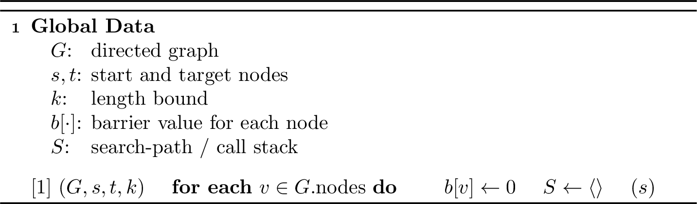
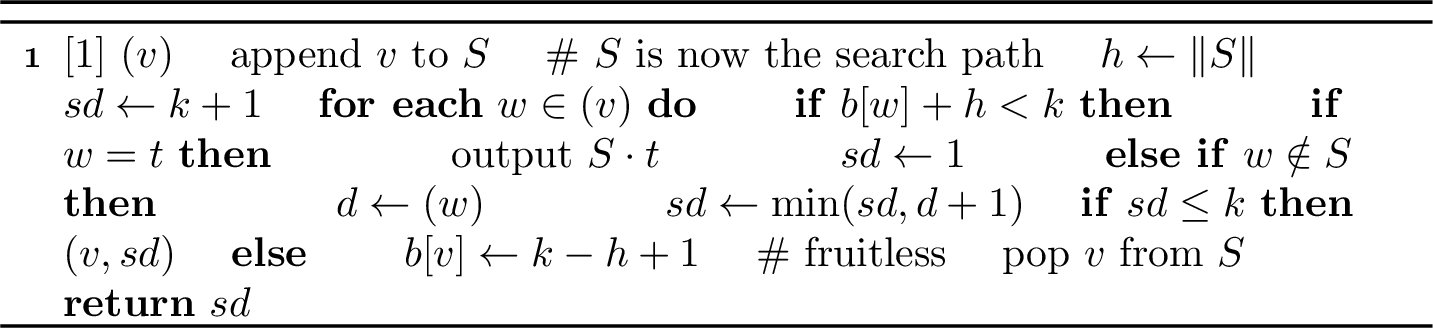
We give a short overview of the algorithm. All details will be elaborated upon and proven in later sections. After initialization, \(\mathop{\mathrm{\mathrm{\small BS-DFS}}}(G, s, t, k)\) sets the search-path stack \(S\) empty and calls \(\mathop{\mathrm{\mathrm{\small Search}}}(s)\), starting the recursive depth-first exploration of \(G\). A call \(\mathop{\mathrm{\mathrm{\small Search}}}(v)\) (2) appends its node \(v\) to \(S\) (line 2), so that during the call \(S = (s = v_0, v_1, \dots, v_h = v)\) is the current search path, of length \(h = \|S\|\) (line 3); it mirrors the \(\mathop{\mathrm{\mathrm{\small Search}}}\) call stack. We name a call by its current node, \(\mathop{\mathrm{\mathrm{\small Search}}}(v)\); in the prose we write \(P\) for the contents of \(S\) at entry (the prefix, before \(v\) is appended), \(Pv = P \cdot v\) for the search path while the call is active, and \(Pvw\) for the search path of the child call on a successor \(w\). These are snapshots of the single stack \(S\) at successive moments. The successors \(w\) of \(v\) are examined (line 5), each guarded by a pruning condition \(b[w] + h < k\) (line 6) to avoid excessive fruitless searches. When a successor equals the target (\(w = t\)), the path \(S \cdot t\) is output and \(sd\) (“shortest distance”) is set to \(1\) (lines 8–9); otherwise a recursive search \(\mathop{\mathrm{\mathrm{\small Search}}}(w)\) is performed at the successor \(w\) (line 11). During the for-loop, \(sd\) tracks the shortest path length to \(t\) found via an edge to \(t\) or in any child search (line 12). After the for-loop, \(sd \le k\) marks the fruitful case (line 13), in which output was produced, and \(sd = k + 1\) the fruitless case (line 15). In the fruitful case, \(\mathop{\mathrm{\mathrm{\small Fruitful}}}(v, sd)\) (3) assigns \(b[v] \gets sd\) and propagates distance values \(d\) backwards to predecessors in a breadth-first cascade; in the fruitless case, \(b[v] \gets k - h + 1\) (line 16). Finally, \(\mathop{\mathrm{\mathrm{\small Search}}}(v)\) pops \(v\) from \(S\) (line 17), restoring the prefix, and returns \(sd\) (line 18).

3.1.0.1 Note for implementations.

The algorithm maintains the current search path in a single stack \(S\), appending a node upon entry to \(\mathop{\mathrm{\mathrm{\small Search}}}\) and removing it immediately before returning. By augmenting the stack with an auxiliary boolean on-stack flag for each node, both stack operations and the membership tests — \(w \notin S\) in \(\mathop{\mathrm{\mathrm{\small Search}}}\) and \(p \notin S\) in \(\mathop{\mathrm{\mathrm{\small Fruitful}}}\) — can be performed in \(O(1)\) time. The resulting space requirement is \(O(n+m)\).

3.2 \(\mathop{\mathrm{\mathrm{\small BS-DFS}}}\) for Simple \(s\)-Cycle Search↩︎

The procedure \(\mathop{\mathrm{\mathrm{\small Search}}}\) is formulated in an edge-oriented manner. This leads to the following reduction.

3.3 Pre-processing for Finding All Simple Cycles↩︎

Enumerating all simple cycles of length at most \(k\) in \(G=(V,E)\) — not only those through a fixed node — reduces to the single-node case by a pre-processing step. Order the nodes as \(V = \{v_1, v_2, \dots, v_n\}\) and let \(G^i\) denote the subgraph of \(G\) induced by \(V^i = \{v_i, v_{i+1}, \dots, v_n\}\). Every simple cycle \(C\) of length \(\le k\) occurs in exactly one of these graphs as a cycle through the distinguished node, namely in \(G^i\) for the smallest index \(i\) among the nodes of \(C\).

Preprocessing creates a list \(L\) of all indices \(i\) where \(G^i\) contains at least one simple \(v_i\)-cycle of length \(k\) or less. For each graph \(G^i\), this can be decided by a distance-limited breadth-first search from \(v_i\), testing if any predecessor of \(v_i\) can be reached within distance \(k-1\). This takes \(O(n+m)\) time per graph and the total pre-processing time is \(O(n(n+m))\). After pre-processing, for all \(v_i \in L\), \(\mathop{\mathrm{\mathrm{\small BS-DFS}}}(G^i, v_i, v_i, k)\) is executed, producing all simple cycles in \(G\) of length \(\le k\).

Further pre-processing is common for reducing the practical runtime [3], [10], [12]: reducing \(G^i\) to the strongly connected component containing \(v_i\), or removing nodes \(x\) with \(dist^{G^i}(v_i, x) + dist^{G^i}(x, v_i) > k\), which cannot lie on any qualifying cycle.

In the remainder of the paper we focus on the path-search setting and, unless stated otherwise, assume that \(s \neq t\). The assumption is not restrictive: the case \(s = t\) is covered verbatim by 2 (), and it lets us state path-avoidance conditions without endpoint exemptions.

3.4 Basic Observations↩︎

The following elementary observations capture structural properties and invariants of \(\mathop{\mathrm{\mathrm{\small BS-DFS}}}\) that will be used repeatedly in the correctness proofs. Their proofs are straightforward and are therefore omitted.

1. Every search path is simple.

2. Every output path is a simple \(s\)-\(t\)-path.

3. Every search path occurs at most once.

4. No output path is produced more than once.

5. Every return value \(sd\) is non-negative.

6. During a call \(\mathop{\mathrm{\mathrm{\small Search}}}(v)\), the barrier value \(b[v]\) can be modified only by that call’s final assignment.

7. For the source, \(b[s]=0\) remains during execution until the final assignment of the initial call.

8. For the target, \(b[t]=0\) remains throughout the execution, except in the case \(s=t\) where [obs:source-barrier] applies.

9. In \(\mathop{\mathrm{\mathrm{\small Fruitful}}}\), every cascade assignment strictly decreases the barrier value of the updated node.

4 Soundness↩︎

In this section we show that every output produced by \(\mathop{\mathrm{\mathrm{\small BS-DFS}}}(G, s, t, k)\) is a simple \(s\)-\(t\)-path of length \(\le k\) in \(G\).

Summarizing all above claims, we conclude that the algorithm produces only valid output (soundness):

We close this section by stating two corollaries.

5 Completeness↩︎

In this section we prove the completeness of \(\mathop{\mathrm{\mathrm{\small BS-DFS}}}(G,s,t,k)\), namely that it produces every simple \(s\)-\(t\)-path in \(G\) of length at most \(k\). The proof is based on a graph-local property of the barrier values, called edge-consistent labelling. We first introduce this property and establish its basic consequences. We then show that it is maintained throughout the execution of \(\mathop{\mathrm{\mathrm{\small BS-DFS}}}\), and finally use it to prove completeness.

5.1 Edge-Consistent Labelling↩︎

The following discussion is naturally interpreted through the framework of heuristic search. The barrier value \(b[x]\) may be viewed as an estimate of the remaining distance from \(x\) to the target \(t\), while the search-path length \(h\) represents the cost already incurred. In the terminology of \(A^*\)-search [19], \(h\) plays the role of the \(g\)-value and \(b[x]\) the role of a heuristic estimate. The pruning condition \(b[w] + h < k\) is then \(f\)-value pruning against a budget: a successor is explored only when the estimated total cost \(g + h\) stays below \(k\). The edge-consistent labelling is precisely the consistency (monotonicity) condition \(h(x) \le w(x,y) + h(y)\) of \(A^*\), with unit edge weights \(w \equiv 1\) and required only for edges whose two endpoints lie outside the current search path.

The completeness argument then follows the classical pattern. Consistency implies admissibility: the barrier never overestimates the true remaining distance to the target. We shall show that \(b[x]\le dist_S(x,t)\), where \(S\) is the current search path. Consequently, whenever a simple \(s\)-\(t\)-path of length at most \(k\) exists through a successor, the pruning condition cannot exclude that successor. Every feasible path therefore survives all pruning tests and is eventually generated.

The principal difference from classical heuristic search is that the heuristic is not fixed. In \(A^*\), consistency is a static property verified once for a given heuristic. In contrast, the barrier values of \(\mathop{\mathrm{\mathrm{\small BS-DFS}}}\) are continually modified during the search: fruitless returns raise barriers, while update cascades may lower them. Consistency is therefore not a precondition but an invariant that must be preserved under every state update. Establishing this invariant constitutes the main technical component of the completeness proof. In this respect \(\mathop{\mathrm{\mathrm{\small BS-DFS}}}\) is closer to learning real-time \(A^*\) [20], where the heuristic is likewise refined as the search proceeds, than to the static algorithm.

Specialized to \(y = t\) with \(b[t] = 0\), the distance bound reads \(b[x] \le dist_S(x,t)\): the barrier never overestimates the true remaining distance — admissibility in the sense of \(A^*\). What makes the analysis nontrivial is that \(S\) changes during the search, and admissibility is a property of a given \(S\); the remainder of this section tracks how the three kinds of state change — barrier writes, path pushes, and path pops — affect it.

We stress that edge-consistency is sufficient but stronger than necessary: completeness needs only that the barrier be admissible (\(b[x] \le dist_S(x,t)\)) at the moment each successor is tested, which is all 8 () uses. Any labelling that under-estimates the remaining distance at that instant therefore yields completeness, edge-consistent or not; we maintain the stronger, local edge-consistency only because it implies admissibility incrementally across the search’s writes, pushes, and pops.

5.2 Fruitless and Fruitful Bounds↩︎

The following lemmas characterize how a single search call affects the barrier values. A fruitless call can only increase its own barrier (9), and while a call remains fruitless no barrier value decreases anywhere in its recursion subtree (10). Conversely, a fruitful call returns a value that is at least the true distance to the target (11), and the ensuing update cascade assigns barrier values that are likewise lower bounded by the corresponding distances to \(t\) (12). The complementary upper bounds, which together imply that cascade updates coincide with the exact distances, are established in 5.3.

Recall from 3 that during a call \(\mathop{\mathrm{\mathrm{\small Search}}}(v)\) (2) the search path is the current stack snapshot \(Pv=(s=v_0,\ldots,v_h=v)\) where \(h = \|Pv\|\), and that \(P\) denotes the prefix of this path at the time the call is entered. Since Observation [obs:target-barrier] shows that \(b[t]=0\) throughout the execution, every lemma below may assume this property without further mention.

5.3 Fruitful Cascades↩︎

We now isolate the only state transition that can violate admissibility. Barrier writes cannot do so: a fruitless or fruitful return modifies the barrier of a node that still lies on the current search path, and admissibility places no restriction on such nodes. Likewise, a cascade only decreases barrier values (Observation [obs:cascade-lowers]), so it cannot raise an admissible value above its distance bound.

A push enlarges the forbidden set, which only relaxes the edge-consistency constraints. The remaining transition is a pop: when \(\mathop{\mathrm{\mathrm{\small Search}}}(v)\) removes \(v\) from the search path, the forbidden set shrinks from \(Pv\) to \(P\), and an edge \((x,y)\) is newly constrained w.r.t.\(P\) exactly when \(v \in \{x,y\}\) — removing \(v\) changes the constrained/exempt status of no other edge. Re-establishing edge-consistency at a pop is therefore a local obligation on the edges incident to \(v\). The next lemma discharges the incoming edges and the case \(y = v\); the single family it defers — edges leaving \(v\) — is handled in 18 (), and is the only point where the exact fruitful value is needed.

5.4 Edge-Consistency of \(\mathop{\mathrm{\mathrm{\small BS-DFS}}}\)↩︎

It suffices to show that \(\mathop{\mathrm{\mathrm{\small BS-DFS}}}\) keeps its labelling edge-consistent w.r.t.the path after the pop; completeness then follows. By the preceding subsection the only nontrivial obligation at a pop of \(v\) is on the edges leaving \(v\), and discharging it needs the cascade to have deposited the exact distance — equivalently, that the fruitful return value satisfies \(sd = dist_{Pv}(v,t)\), which in turn needs the shortest completion to have been produced. Completeness, the exact value, and preservation at the pop are thus mutually dependent and are established together, by a single induction on the search recursion, well-founded by 6 ().

For each call \(\mathop{\mathrm{\mathrm{\small Search}}}(v)\) the induction carries the following clauses:

1. completeness of the call (15);

2. the exact fruitful value (16);

3. global monotonicity (17);

4. preservation across the call (18).

In each of the four lemmas below the induction hypothesis is that all four claims hold for every call nested strictly within the current \(\mathop{\mathrm{\mathrm{\small Search}}}(v)\). A pruning test that a budget-respecting path must survive is discharged directly by 8 (); no global completeness statement is invoked inside the induction.

5.5 Completeness of \(\mathop{\mathrm{\mathrm{\small BS-DFS}}}\)↩︎

We have seen that edge-consistency w.r.t.the current search path holds throughout the execution of \(\mathop{\mathrm{\mathrm{\small BS-DFS}}}(G,s,t,k)\). This is the global reading of 18 (): starting from \(b \equiv 0\) (edge-consistent w.r.t.the empty path), the single call \(\mathop{\mathrm{\mathrm{\small Search}}}(s)\) is entered with the invariant, and the lemma shows each call preserves it w.r.t. the path after its node is popped; chaining over the call tree gives the invariant at every point. We close with the main theorems in this section.

6 Delay Bounds↩︎

For delay analysis, the entire \(\mathop{\mathrm{\mathrm{\small BS-DFS}}}(G,s,t,k)\) execution is partitioned into a sequence of intervals. A new interval starts when the algorithm begins or whenever output is produced. An interval ends with the next output or when the algorithm terminates.

Let the delay of an interval be the number of elementary steps executed by the algorithm in that interval. We will show that for a graph \(G\) with \(n\) nodes and \(m\) edges and a given length bound \(k \in \mathbb{N}^+\), the maximum delay of \(\mathop{\mathrm{\mathrm{\small BS-DFS}}}(G,s,t,k)\) is bounded by \(O(k(n+m))\). Before doing so, we will analyze the execution of \(\mathop{\mathrm{\mathrm{\small BS-DFS}}}\) within an interval in greater detail, see also 4.

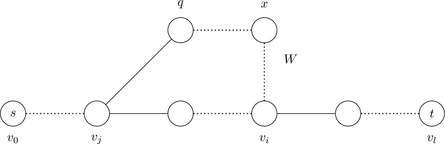
We index the intervals \(\tau = 1, 2, \dots\) in order of occurrence. The output path opening interval \(\tau\) is called its spine, denoted \(S_\tau = (s = v_0, v_1, \dots, v_l = t)\). The first interval is opened by the start of the execution rather than by an output; we set \(S_1 = \emptyset\). Symmetrically, the execution’s end closes the terminal interval \(T\) without an output; we set \(S_{T+1} = \emptyset\). Sums indexed by an empty spine are zero.

When \(v_l = t\) is reached, the spine path is output. Next, the \(\mathop{\mathrm{\mathrm{\small Search}}}\) call stack unwinds one level, leaving \(v_{l-1}\) on top. \(\mathop{\mathrm{\mathrm{\small Search}}}(v_{l-1})\) continues enumerating the successors of \(v_{l-1}\) after \(v_l\) in the successor list and recurses into those that pass the pruning condition. If one such sibling search returns fruitful, the next \(s\)-\(t\)-path was produced during that search and the output immediately starts the next interval, before the fruitful sibling search returns. Otherwise, all sibling searches at \(v_{l-1}\) return fruitless. Since \(\mathop{\mathrm{\mathrm{\small Search}}}(v_{l-1})\) itself is fruitful (it produced \(v_l\) on the spine), \(b[v_{l-1}]\) is assigned and the cascade \(\mathop{\mathrm{\mathrm{\small Fruitful}}}(v_{l-1}, sd)\) runs. The stack then unwinds to \(v_{l-2}\) and the procedure repeats.

This continues until either (a) at some spine level \(v_j\) a sibling search \(\mathop{\mathrm{\mathrm{\small Search}}}(q)\) returns fruitful, producing the next \(s\)-\(t\)-path \(S_{\tau+1} = (v_0, \dots, v_j, q, \dots, t)\); or (b) the unwinding exhausts level \(v_0 = s\) and the algorithm terminates. In case (a), the spine node \(v_j\) is the deepest stack level that remains continuously occupied across the two outputs; we call it the lowest common ancestor (LCA) of \(S_\tau\) and \(S_{\tau+1}\). The spine prefix \((v_0, \dots, v_j)\) is shared between the two paths; the suffixes \((v_{j+1}, \dots, v_l)\) and \((q, \dots, t)\) are disjoint.

4 additionally depicts a deeper spine node \(v_i\) whose cascade \(\mathop{\mathrm{\mathrm{\small Fruitful}}}(v_i, sd)\) deposits a barrier value \(b[x]\) at some node \(x\) off the spine; the witness path \(W\) from \(x\) via \(v_i\) to \(t\) plays a central role in the interval-ending argument below.

6.1 Barrier Events↩︎

Consider the sequence of barrier assignments in an interval. For a node \(x\), we classify the assignments to \(b[x]\):

• S-event: \(b[x] \gets k - h + 1\), assigned in a fruitless \(\mathop{\mathrm{\mathrm{\small Search}}}(x)\);

• F-event: \(b[x] \gets sd\), the origin write at the start of a cascade \(\mathop{\mathrm{\mathrm{\small Fruitful}}}(x, sd)\) invoked from a fruitful \(\mathop{\mathrm{\mathrm{\small Search}}}(x)\).

• U-event: \(b[x] \gets d + 1\), the predecessor write inside some cascade call \(\mathop{\mathrm{\mathrm{\small Fruitful}}}(q, d)\) with \(q \in \mathop{\mathrm{\mathrm{succ}}}(x)\), under the guard \(b[x] > d + 1\);

There are no other types of events, and no other function call during \(\mathop{\mathrm{\mathrm{\small BS-DFS}}}(G, s, t, k)\) visits a node \(x\) without assigning \(b[x]\).

Note that there is at most one F-event per node per interval, namely when \(\mathop{\mathrm{\mathrm{\small Search}}}(v_i)\) at a spine node \(v_i\) returns fruitful.

We consider the sequence of S- and U-events occurring in an interval and divide it into one or more homogeneous blocks of events of the same type, separated by event-type transitions. Note that the order of events, due to recursion, can differ from the function-call order, since the barriers are written in postfix order before return.

Fruitful work and boundary work are thus symmetric: the former is indexed by the spine \(S_\tau\) that opens the interval, the latter by the spine \(S_{\tau+1}\) that closes it.

6.2 Sharpening the Constant↩︎

3 charges every interval the full \(3(k+1)(n+m)\). Two refinements lower the effective constant: the first interval is genuinely cheaper, and across an output boundary the trailing and leading fruitless work of consecutive intervals can be amortized. We record both, the former as a proven sharpening and the latter as a conjecture with its residual obligation made precise. Both rest on the global monotonicity clause of the joint induction (17 ()). This lemma is a statement about a completed call: a fruitful call may lower barriers transiently while its cascade is in flight, but never below the value held at the call’s entry. It does not bound barriers at instants interior to a call still on the stack — precisely the instants that an output boundary straddles — which is why it sharpens the first interval but leaves the cross-boundary amortization a conjecture.

6.2.0.1 The first interval.

The first interval starts at the entry of \(\mathop{\mathrm{\mathrm{\small Search}}}(s)\) and ends at the first output, which is produced inside the for-loop of the deepest spine node, before that call returns fruitful. No \(\mathop{\mathrm{\mathrm{\small Search}}}\) call has yet returned fruitful, so no \(\mathop{\mathrm{\mathrm{\small Fruitful}}}\) cascade has run: the interval contains neither F-events nor U-events. By 23 () the event sequence at each node is a single S-block, and only the fruitless-work and boundary-work terms of 3 () contribute. The first interval therefore has delay at most \(k(n+m) + (k + m) \le (k + 1)(n + m)\), a factor \(3\) below the general bound.

6.2.0.2 Amortizing across output boundaries (conjecture).

Fix a node \(x\) and read its S- and U-events across the whole run, ignoring the output boundaries. Within one interval the sequence has the form \(S^* U^* S^*\) (23 ()). An output is not a barrier event at \(x\), so the trailing S-block of interval \(\tau\) and the leading S-block of interval \(\tau+1\) are separated only by the output boundary — unless a barrier-lowering write to \(x\) falls between them. The only lowering writes are U-events (guarded cascade decreases) and the F-event origin of \(x\)’s own fruitful call (which ends \(x\)’s interval). Thus, if no U-event at \(x\) occurs across the boundary, the two S-blocks form one contiguous strictly increasing chain, which by 19 () still has at most \(k\) events.

This suggests counting the cumulative fruitless work over the first \(p\) outputs by maximal monotone S-runs rather than per-interval S-blocks. Each node’s S-events decompose into runs delimited by its lowering writes, every run of length at most \(k\); the number of runs at \(x\) is \(1\) plus the number of lowering writes to \(x\). Charging each run to the U-event (or interval-ending F-origin) that closes it yields, over \(p\) outputs, \(p\) S-runs interspersed with the \(p-1\) U-blocks of the interior boundaries, in place of the \(2p\) S-blocks and \(p\) U-blocks counted interval-by-interval. Empirically the per-output delay settles near \(2k(n+m)\) rather than \(3k(n+m)\), consistent with this picture.

We state the amortized bound as a conjecture, since the charging argument above trades the clean per-interval accounting of 3 () for a global S\(\leftrightarrow\)U bookkeeping whose constant we have not established rigorously; the worst-case per-interval bound of 3 () remains the proven guarantee.

We close this section with a delay bound for enumerating all simple cycles.

7 Edge-Consistent Variants of \(\mathop{\mathrm{\mathrm{\small BS-DFS}}}\)↩︎

The pruning of \(\mathop{\mathrm{\mathrm{\small BS-DFS}}}\) is governed entirely by the barrier values, and the only freedom in the algorithm is how the algorithm revises the barriers. Several schemes share the same skeleton — the recursive search, and the pruning condition \(b[w] + h < k\) — and differ only in the barrier post-processing after recursion. We call a scheme edge-consistent if it maintains edge-consistency with respect to the current search path at every quiescent point, i.e.whenever control is in \(\mathop{\mathrm{\mathrm{\small Search}}}\) and not inside a fruitful cascade; by 8 () every edge-consistent scheme is complete. The tight scheme of the original \(\mathop{\mathrm{\mathrm{\small BS-DFS}}}\) is one extreme. We record three further points on the spectrum.

7.1 The Trivial Scheme↩︎

Leave every barrier at \(0\): the algorithm does not manage barriers at all. Then \(b \equiv 0\) is trivially edge-consistent w.r.t.any search path, so the scheme is complete — it is plain depth-first search with the length cutoff \(h < k\), performing no barrier-based pruning. Soundness and completeness obviously hold, but there is no polynomial delay bound: if the depth-first search first descends into a complete subgraph of size \(k-1\) not containing the target \(t\), it traverses \(\Theta((k-2)!)\) partial paths before producing any output.

7.2 The Loose Scheme↩︎

The loose scheme keeps the backward cascade of the fruitful case but replaces the distance values it deposits by \(0\). That is, 3 () is replaced by \(\mathrm{\small Reset}(v)\): a breadth-first traversal backwards from \(v\) over predecessors, restricted to nodes off the search path, setting every visited barrier to \(0\).

The guard \(b[p] \ne 0\) cannot be tightened to the depth-aware \(b[p] > d + 1\) of the tight cascade. Because \(\mathrm{\small Reset}\) records no distance information, edge-consistency is preserved only by resetting the entire reachable off-path cone: stopping the propagation early would leave a node with a positive barrier adjacent to a node reset to \(0\), breaking consistency. The full cone is the price of discarding distances, and it is why the loose scheme has no delay advantage — a point we return to below.

The conceptual value of the loose scheme is that it isolates which part of the tight correctness proof is essential. We show it is edge-consistent; completeness then follows from 8 () as for any edge-consistent scheme. As in the tight case, a cascade transiently violates edge-consistency while in flight and restores it on completion, so the statements below concern quiescent points.

The case that dominates the tight proof disappears. A fruitful node ends its cascade with \(b[v] = 0\) (line 2 of 5), so every outgoing edge \((v,y)\) satisfies \(b[v] \le b[y] + 1\) as \(0 \le b[y] + 1\). This is precisely the case for which the tight proof needs the exact value \(sd = dist_{Pv}(v,t)\), and hence completeness; here it is free. The only case requiring an argument is an off-path edge \((x,y)\) whose head \(y\) was reset to \(0\), settled by the following closure property.

If \((x,y)\) is off-path with \(y \in R\), then \(x\) is an off-path predecessor of a reset node, so \(b[x] = 0\) and \(b[x] \le b[y] + 1\). The configuration one might fear — a fruitless node \(x\) with a high barrier pointing into a freshly-reset \(y\) — cannot arise, because the cascade reaches \(x\) through \(y\) and resets it too. Off-path edges with both endpoints untouched inherit consistency from before the cascade, and the edges that the pop of \(v\) newly constrains are consistent for the same two reasons (\(b[v] = 0\) outgoing, 24 with \(y = v\) incoming). The fruitless case and the push are as in the tight scheme. Hence, the loose scheme is edge-consistent, and the four-way joint induction of 5 collapses to a single inequality invariant: no exact-value claim, no coupling to completeness.

7.2.0.1 Delay.

Both, tight and loose schemes are complete and deterministic and scan successors in the same order. Since pruning removes only output-free subtrees, each emits its outputs in lexicographic path order; hence the two output sequences are equal. Therefore, the intervals correspond one-to-one and the spine paths coincide. The fruitful calls returning within an interval are exactly the calls along its spine, so the fruitful and boundary work of the tally in 3 () is identical in both schemes.

Nonetheless, there can be more fruitless searches within an interval, because some barriers are reset to 0 instead of being updated to the tight bound and 23 () fails for the loose scheme, violating executions were observed experimentally. We leave the delay bound for the loose scheme as an open question.

7.3 The Lazy Scheme↩︎

The loose scheme (7.2) discards distance information but still incurs, at every fruitful step, the cost of a backward cascade over the entire reachable off-path cone. The lazy scheme retains the same coarse reset to \(0\) while deferring the cascade. A fruitless node registers itself in a dependency list at each of its successors, and a later fruitful node consumes those lists, clearing only the nodes that registered through it. Distance information is still discarded—a fruitful node is reset to \(0\) exactly as in the loose scheme— so the lazy scheme inherits the loose scheme’s simple correctness argument, which does not rely on exact distance values. The only difference is which barriers are cleared by a fruitful step, and when they are cleared.

Each node \(x\) now carries, in addition to its barrier \(b[x]\), a dependency list \(B[x] \subseteq V\). When a call \(\mathop{\mathrm{\mathrm{\small Search}}}(v)\) returns fruitless at depth \(h\), it performs the usual assignment \[b[v] \gets k-h+1\] and additionally inserts \(v\) into \(B[w]\) for every successor \(w \in \mathop{\mathrm{\mathrm{succ}}}(v)\) (the registration step, line [line:register]). The fruitful case runs \(\mathrm{\small Update}(v)\) instead of the loose reset.

The barrier \(b[\cdot]\) is initialized to \(0\) and the dependency lists \(B[\cdot]\) to \(\emptyset\); the rest of \(\mathop{\mathrm{\mathrm{\small BS-DFS}}}\) (3) is unchanged. The clear of \(B[v]\) in line [line:clear] couples de-registration with clearing: a node is removed from a dependency list exactly when the cascade that clears its barrier passes through. Without it the lists would only grow, accumulating stale entries; with it they record precisely the nodes whose positive barrier is still in force, which is what the analysis below exploits.

Gupta and Suzumura [10] pair lazy registration with the tight (distance-depositing) fruitful case; but that combination is not always complete, see [13]. The lazy scheme is complete precisely because it is coarse: it resets to \(0\), so no exact distance need be maintained, and registration only has to control which nodes are reset.

Next, we show completeness of the lazy scheme.

7.3.0.1 The registration invariant.

The mechanism rests on a single edge-local invariant.

7.3.0.2 Edge-consistency.

We show the lazy scheme is edge-consistent w.r.t.the current search path at every point at which control is not inside an \(\mathrm{\small Update}\) cascade; completeness then follows from 8 () exactly as for the loose scheme. As before, a cascade transiently breaks edge-consistency and restores it on completion, so the statement concerns these quiescent points.

The induction over the run is identical to the loose case (7.2) on entry, fruitless assignment, and push; only the fruitful cascade differs, and there 25 replaces the loose closure property. The crux is the following.

With 26, the fruitful cascade preserves edge-consistency just as the loose reset did. Consider an off-path edge \((x,y)\) after \(\mathrm{\small Update}(v)\) completes. If \(b[y]\) was cleared by the cascade, then \(\mathrm{\small Update}(y)\) was invoked. Since \(x\) is an off-stack predecessor of \(y\), 26 implies that \(b[x]=0\) from the moment \(\mathrm{\small Update}(y)\) returns. Therefore, \(b[x]=0 \le b[y]+1.\) If \(b[y]\) was not cleared, then the edge retains the consistency it had before the cascade. Indeed, \(b[x]\) can only have decreased during the cascade, so any inequality \(b[x] \le b[y]+1\) that held before the cascade continues to hold afterward. The fruitful node itself ends with \(b[v]=0\). Hence, its outgoing edges are consistent for free. Its incoming edges are covered by 26 with \(y=v\), for exactly the same reason as in the loose scheme. The fruitless case, the push, and the pop are as in the loose scheme. Thus, the lazy scheme is edge-consistent at every quiescent point of the execution. By 8 (), it follows that the algorithm produces every simple \(s\)-\(t\)-path of length \(\le k\).

7.3.0.3 Delay.

Like the loose scheme, the lazy scheme discards distance information and resets fruitful nodes to \(0\). Consequently, it offers no proven delay improvement over the tight scheme, and its interval-delay complexity remains open. Its main interest is structural. It demonstrates that the fruitful cascade can be driven lazily, through dependency lists accumulated during fruitless search and consumed upon success, while still preserving edge-consistency. More importantly, it shows that correctness depends on the coarse reset itself rather than on the lazy bookkeeping. Indeed, it is precisely the combination of lazy registration with a tight fruitful case that fails in \(\mathrm{\small CYCLE\_SEARCH}\), as shown in [13]. The lazy scheme remains complete because it abandons exact distance information and resets fruitful nodes to \(0\).

8 Analyzing the \(\mathrm{\small BC-DFS}\) Algorithm↩︎

Now that we have established the correctness of \(\mathop{\mathrm{\mathrm{\small BS-DFS}}}\) and its variants, we turn to the \(\mathrm{\small BC-DFS}\) algorithm of Peng et al. [11], [12]. We show that \(\mathrm{\small BC-DFS}\) is not complete and identify a corresponding gap in its correctness proof. The crucial difference between \(\mathrm{\small BC-DFS}\) and \(\mathop{\mathrm{\mathrm{\small BS-DFS}}}\) lies in the handling of fruitful returns. In \(\mathop{\mathrm{\mathrm{\small BS-DFS}}}\), a fruitful call always performs an unconditional barrier update through \(\mathop{\mathrm{\mathrm{\small Fruitful}}}\) (3). By contrast, \(\mathrm{\small BC-DFS}\) propagates a fruitful value only when a guard condition is satisfied. Its update procedure, reproduced in [alg:UpdateBarrier], assigns a value \(l\) to a node \(u\) only if \(b[u] > l\). Moreover, if the guard fails for the initial call to \(\mathrm{\small UpdateBarrier}\), the entire update cascade is skipped. This behavior appears both in the conference version [11] and in the journal version [12]. As we show below, suppressing the cascade in this way can leave stale barrier values in place and may cause valid paths to be pruned.

8.1 A Counter-Example to \(\mathrm{\small BC-DFS}\) Completeness↩︎

Skipping the update cascade can violate edge-consistency and thereby destroy completeness. This is demonstrated by the graph \(X\) depicted in 8.

The directed graph \(X\) is assumed to be stored in adjacency list format in alphabetical order. It contains the following simple paths starting at node \(A\), terminating at node \(E\) and having length 4 or less:

However, when \(\mathrm{\small BC-DFS}(G,s,t,k)\) with \(G=X\), \(s=A\), \(t=E\), \(k=4\) is executed, it will only find the first two paths and miss the third one. An execution trace for the counter-example is given in [list:bcdfs-counterexample-X].

While \(B\) is on the search path, the fruitless searches of \(C\) and \(D\) raise their barriers to \(b[C] = b[D] = 3\). When the search of \(B\) then returns fruitful, \(\mathrm{\small BC-DFS}\) skips its \(\mathrm{\small UpdateBarrier}\) cascade — visible as the absence of any update at search(B) fruitful, the barrier vector being unchanged across the pop of \(B\). The relaxations that would lower \(b[C]\) and \(b[D]\) along the edges \((C, B)\) and \((D, B)\) are therefore never performed, and \(b[D] = 3\) persists.

The stale barrier is fatal one step later. When the search path becomes \((A, C)\), the successor \(D\) is examined at depth \(h = 1\); the pruning test fails, since \(b[D] + h = 3 + 1 = 4 \ge k\), so \(D\) is pruned (trace: D pruned (4 >= k)). The only \(A\)-\(E\)-path through this edge, \((A, C, D, B, E)\), is thereby lost: \(\mathrm{\small BC-DFS}\) outputs \((A, B, E)\) and \((A, C, B, E)\) but misses the valid path \((A, C, D, B, E)\) proving that the algorithm is not complete. The same stale \(b[D] = 3\) had already pruned \(D\) at the deeper path \((A, C, B)\), where \(b[D] + h = 3 + 2 = 5 \ge k\) (trace: D pruned (5 >= k)).

Additional counter-examples were found experimentally by searching small random graphs, of which \(X\) is among the smallest. Moreover, infinitely many counter-examples can be obtained by suitable augmentations of \(X\).

8.2 Proof Analysis of \(\mathrm{\small BC-DFS}\) Completeness↩︎

The incompleteness of \(\mathrm{\small BC-DFS}\) is not merely an implementation issue. Upon closer inspection, the correctness proof contains a gap precisely at the point where the algorithm fails on the counter-example above. The proof of Theorem 1 in [11], [12] argues that “for any vertex \(u\), \(u.\mathrm{bar}\) is correctly maintained in Algorithm \(\mathrm{\small BC-DFS}\)”. The argument distinguishes two cases, depending on whether the vertex \(x\) coincides with a vertex \(v\). For the case \(x \ne v\), the proof explicitly describes how barrier values are propagated along the path \(p(u \to x)\). For the case \(x = v\), however, it states only that “the proof is similar” and does not provide the corresponding argument. Our counter-example falls precisely into this omitted case. When \(x=v\) and \(N=\emptyset\), the propagation argument through the vertices of \(N\) becomes vacuous. At the same time, the guard \(u.\mathrm{bar} > l\) in \(\mathrm{\small UpdateBarrier}\) may prevent the relaxation from reaching \(u\). Consequently, stale barrier values can remain in place and valid paths may be pruned, exactly as observed in the counter-example. Thus, the failure exhibited by the counter-example corresponds precisely to the case that is not established in the published proof.

8.3 Proof Analysis of \(\mathrm{\small BC-DFS}\) Time Complexity↩︎

We also identify a gap in the time-complexity argument of \(\mathrm{\small BC-DFS}\). Beyond its relevance to the complexity analysis, the discussion reveals several interesting structural properties of the algorithm. In [11], [12], the central step in the proof of Theorem 2, which states that “\(\mathrm{\small BC-DFS}\) is a polynomial-delay algorithm with \(O(km)\) time per output”, is the following argument:

Suppose a vertex u is unstacked twice and there is no new output in Algorithm 1. Let \(S1\) and \(S2\) denote the stack size after \(u\) is pushed into the stack at the first and the second time, respectively. We have \(u.bar = k-S1+2\) after u is unstacked at the first time. As there is no new output, the propagation of barrier values will not be invoked. Thus, \(u.bar\) remains the same when \(u\) is pushed to stack at the second time. As \(u\) passes the barrier-based pruning in the second visit, we have \(S2 + u.bar \le k\), and hence \(S2 < S1\).

However, this argument does not correctly account for the interleaving of \(\mathop{\mathrm{\mathrm{\small Search}}}\) and \(\mathop{\mathrm{\mathrm{\small Fruitful}}}\) (here: \(\mathrm{\small UpdateBarrier}\)) calls while the recursion unwinds. As a result, the claimed monotonicity property is false: barrier values may change between two visits of the same vertex even when no new output is produced. A counter-example demonstrating this behavior is depicted in 9.

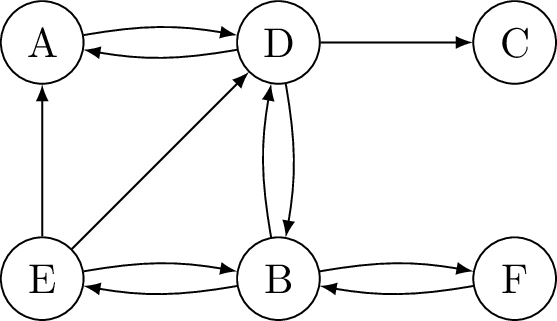
The graph \(Y\) is stored in adjacency-list format in alphabetical order. The complete execution trace of \(\mathrm{\small BC-DFS}(G,s,t,k)\) with \(G = Y\), \(s = E\), \(t = C\), \(k = 6\) is given in [list:bcdfs-counterexample-Y]; the barrier vector \((b[A], b[B], b[C], b[D], b[E], b[F])\) is shown after every step. \(\mathrm{\small BC-DFS}\) produces all three \(s\)-\(t\)-paths \((E, A, D, C)\), \((E, B, D, C)\), and \((E, D, C)\), so completeness is not at issue in this example.

We focus on the node \(F\). In the interval between the second output \((E, B, D, C)\) and the third \((E, D, C)\), two observations are crucial.

First, after the second output \((E, B, D, C)\), the recursion unwinds and the call \(\mathop{\mathrm{\mathrm{\small Search}}}(B)\) at search path \((E, B)\) returns fruitful — its fruitfulness stems from that earlier output, produced within it at greater depth. Its \(\mathrm{\small UpdateBarrier}\) cascade is therefore invoked during the unwind, although no new output has been produced since. The cascade lowers \(b[B] \gets 2\) and \(b[F] \gets 3\). This already contradicts the premise of the quoted argument — that in the absence of a new output “the propagation of barrier values will not be invoked”: between two consecutive outputs, cascades of fruitful calls returning on the spine of the previous output do run.

Second, and within the same interval, \(F\) is unstacked fruitless twice. It is first searched fruitless at search path \((E, B, F)\), of length \(2\), setting \(b[F] \gets 5\); later, after the cascade has reset it to \(3\), it is searched fruitless again at search path \((E, D, B, F)\), of greater length \(3\), setting \(b[F] \gets 4\). So the two stack sizes at which \(F\) is unstacked within one interval satisfy \(S_2 > S_1\), directly contradicting the claimed \(S_2 < S_1\). The barrier of \(F\) is correspondingly non-monotone, moving \(5 \to 3 \to 4\).

Because barrier propagation is invoked without a new output, the step “\(u.bar\) remains the same when \(u\) is pushed to stack the second time” fails, and with it the conclusion \(S_2 < S_1\). The postulated interval delay bound of \(O(km)\) therefore does not follow, and remains open for \(\mathrm{\small BC-DFS}\).

Note that monotonicity does hold in the first interval, where no spine path unwinds and hence no \(\mathop{\mathrm{\mathrm{\small Fruitful}}}\) cascade runs.

The trace for \(\mathop{\mathrm{\mathrm{\small BS-DFS}}}\) on this graph is similar, with additional cascade updates, but the non-monotone assignments to \(b[F]\) are the same. Accounting correctly for the interleaved \(\mathop{\mathrm{\mathrm{\small Search}}}\) and \(\mathop{\mathrm{\mathrm{\small Fruitful}}}\) calls across all intervals is the key point of our \(\mathop{\mathrm{\mathrm{\small BS-DFS}}}\) delay-bound proof.

9 Experiments↩︎

We conducted a preliminary experimental study to quantify the frequency of paths missed by \(\mathrm{\small BC-DFS}\) under random graph models. All experiments were implemented using the NetworkX library [16]. The source code used in the evaluation is publicly available in our GitHub repository [18]. The ground-truth was calculated using a depth-limited depth-first search, not pruned by barrier values, the trivial scheme from 7.1.

We begin with random Erdős–Rényi graphs [21], [22]. For the parameter settings considered, the ratio of missed paths increased with the path-length bound \(k\), exceeding \(10\%\) for \(k=10\); see ¿tbl:table:experiments95er?.

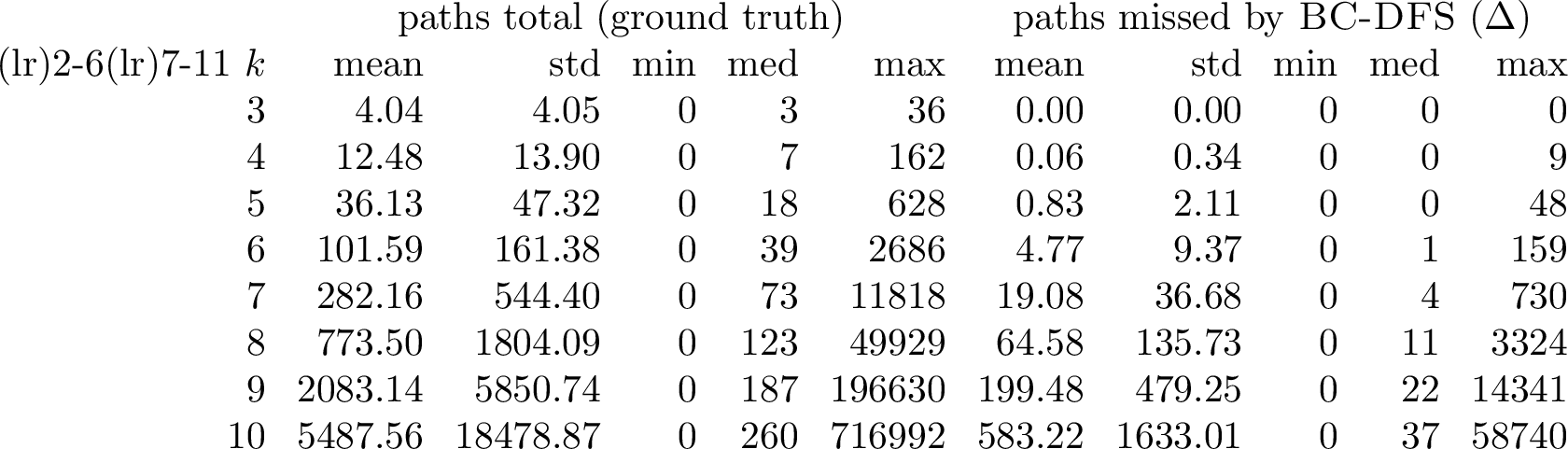
Next, we considered a directed variant of random Watts-Strogatz graphs [23], modelling small-world networks which are closer to the applications intended for BC-DFS. Here, the mean missed path ratio is rapidly growing to over 33% for \(k=10\), see ¿tbl:table:watts-strogatz-experiment?.

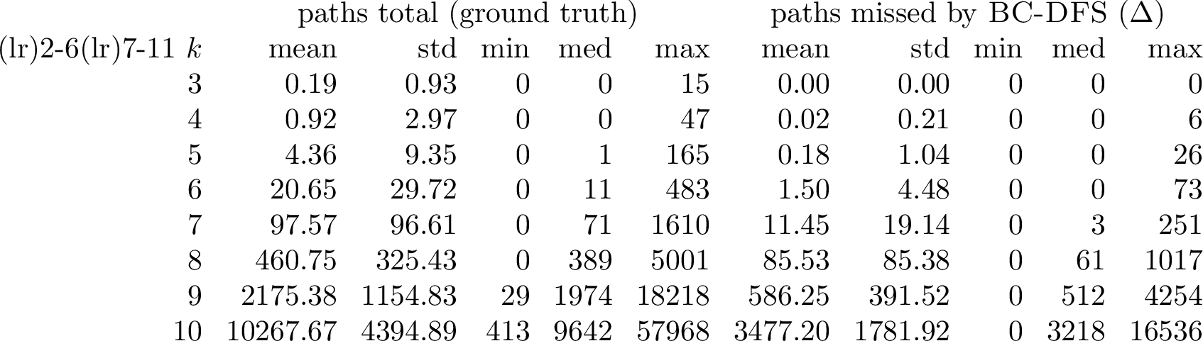
The observed total runtime (wall-clock) for \(\mathop{\mathrm{\mathrm{\small BS-DFS}}}\) and \(\mathrm{\small BC-DFS}\) in these experiments was in the same order of magnitude, with \(\mathop{\mathrm{\mathrm{\small BS-DFS}}}\) using roughly 50% more time than \(\mathrm{\small BC-DFS}\).

To isolate the source of this overhead, we instrumented BC-DFS and a minimal repaired variant, kick-start. The code is identical except for one added line setting \(b[v] \gets k+1\) before the origin call of \(\mathrm{\small UpdateBarrier}\), which makes its first assignment unconditional, mimicking the unconditional \(b[v] \gets sd\) of \(\mathop{\mathrm{\mathrm{\small Fruitful}}}\) (3) while leaving the rest of the BC-DFS implementation untouched. Kick-start produced the ground-truth output on all tested instances. Normalized per output, the two variants perform nearly the same number of search calls and successor probes, whereas BC-DFS performs less than \(6\%\) of kick-start’s predecessor probes and barrier writes; detailed counts are available at [18]. The runtime overhead of the complete algorithms is thus attributable to the proper barrier propagation that completeness requires — work whose omission is precisely what causes the missed outputs quantified above.

10 Conclusion and Outlook↩︎

We presented \(\mathop{\mathrm{\mathrm{\small BS-DFS}}}\), a bounded-scope depth-first search that enumerates all simple \(s\)-\(t\)-paths — and, via node splitting, all simple \(s\)-cycles — of length at most \(k\) in a directed graph, with a worst-case delay of \(O(k(n+m))\) per output (3). The algorithm follows the line of barrier-based methods initiated by Johnson and refined by Peng et al.and by Gupta and Suzumura, but it is built around a single explicit invariant, edge-consistency: the barrier of an off-path node never exceeds one plus the barrier of any off-path successor. Read as a heuristic in the sense of \(A^*\), edge-consistency is exactly admissibility maintained as a search-time invariant, and it yields a transparent completeness argument — an admissible barrier never prunes a path that respects the budget.

The same invariant organizes a whole family of schemes that differ only in how barriers are revised (7). The tight scheme deposits exact distances and pays for its delay bound with a correctness proof in which completeness, the exact return value, and preservation of edge-consistency are mutually entangled. At the other end, the loose (7.2) and lazy (7.3) schemes discard distance information by resetting fruitful nodes to zero; this trades barrier precision for a markedly simpler correctness argument, since zero is the most admissible value and no exact-value claim is needed. The lazy scheme additionally shows that the backward cascade can be driven by dependency lists accumulated during fruitless search and consumed on success, while preserving edge-consistency. We regard this uniform treatment as evidence that edge-consistency is the right abstraction for bounded-scope search, rather than a device specific to one algorithm.

The framework also makes precise where a published algorithm goes wrong. In \(\mathrm{\small BC-DFS}\) (8) a single misplaced guard causes correct barrier relaxations to be silently dropped, breaking edge-consistency and, with it, completeness; our counter-example and the matching gap in the original proof both sit exactly at this point. The accompanying experiments (9) suggest that the resulting missed-path phenomenon is not confined to isolated counter-examples: under the graph models considered, the fraction of missed paths exceeds \(10\%\) and \(33\%\), respectively, already at \(k=10\).

As already proposed for many other path and cycle search algorithms [3], [10]–[12], [14], [15], our \(\mathop{\mathrm{\mathrm{\small BS-DFS}}}\) algorithm can be combined with preprocessing steps like connected component decomposition and breadth-first search for reachability from one or both sides (bidirectional search) to further reduce the search space and improve practical performance.

A practical optimization is to initialize the barrier values in \(\mathop{\mathrm{\mathrm{\small BS-DFS}}}\) by an initial breadth-first search (BFS) from the target node \(t\) in the reverse graph, which sets the initial barrier value of each node to its distance towards \(t\). This allows for more pruning of the search space and thus practically faster execution, especially if the nodes \(x\) which cannot reach \(t\) in budget are initialized with \(b[x] = k + 1\) thus being eliminated from the search.

Several questions remain open. The most concrete is the delay of the loose and lazy schemes: both are complete and edge-consistent, yet resetting to zero re-arms nodes that were already searched fruitlessly within an interval, so the \(O(k(n+m))\) per-output bound of the tight scheme is not known to hold for them, and we make no such claim. Establishing a delay bound for either — or showing that none of the form \(O(k(n+m))\) exists — would sharpen the picture of the precision-versus-analyzability trade-off that the variant spectrum exposes. More broadly, edge-consistency is stated for unit edge weights and a single source and target; extending it to weighted budgets, to multiple targets, or to other structural constraints on the enumerated paths appears to be a natural direction, and one for which the invariant-based proof technique developed here should carry over.

For the tight scheme a linear delay bound is settled; what remains open is its constant. 3 proves \(3(k+1)(n+m)\) per interval, yet the first interval already costs only \((k+1)(n+m)\) (6.2), and the trailing and leading fruitless work of consecutive intervals appears to amortize across output boundaries. We conjecture an amortized per-output delay of \(2k(n+m)\) (1); proving it requires a global S\(\leftrightarrow\)U charging argument that the per-interval accounting does not supply.

A related question is how far edge-consistency can be relaxed: completeness needs only local admissibility (when tested for), which global edge-consistency implies but strictly exceeds, so characterizing the full class of admissible — and hence complete — bounded-scope schemes, edge-consistent or not, is open.

Our experiments are deliberately limited in scope: they use random graph models to investigate the frequency of the missed-path defect of \(\mathrm{\small BC-DFS}\), rather than to provide a thorough benchmark of running time. A broader empirical and comparative study measuring per-output delay on real-world road, social, and similar networks would require substantial code-level optimization. Such engineering work lies outside the focus of this paper and is left to future work.

11 Execution Trace of Counter-Example Graph \(X\)↩︎

S path: barriers  : trace
      : A B C D E :
      : 0 0 0 0 0 : search(A) enter
A     : 0 0 0 0 0 : .search(B) enter
AB    : 0 0 0 0 0 : ..search(C) enter
ABC   : 0 0 0 0 0 : ...search(B) B pruned (in S)
ABC   : 0 0 0 0 0 : ...search(D) enter
ABCD  : 0 0 0 0 0 : ....search(B) B pruned (in S)
ABCD  : 0 0 0 0 0 : ....search(D) fruitless bar[D] := 2 (was 0)
ABC   : 0 0 0 2 0 : ...search(D) exit
ABC   : 0 0 0 2 0 : ...search(C) fruitless bar[C] := 3 (was 0)
AB    : 0 0 3 2 0 : ..search(C) exit
AB    : 0 0 3 2 0 : ..search(D) enter
ABD   : 0 0 3 2 0 : ...search(B) B pruned (in S)
ABD   : 0 0 3 2 0 : ...search(D) fruitless bar[D] := 3 (was 2)
AB    : 0 0 3 3 0 : ..search(D) exit
AB    : 0 0 3 3 0 : ..search(E) enter
ABE   : 0 0 3 3 0 : ...search(E) output ['A', 'B', 'E']
AB    : 0 0 3 3 0 : ..search(B) fruitful
A     : 0 0 3 3 0 : .search(B) exit
A     : 0 0 3 3 0 : .search(C) enter
AC    : 0 0 3 3 0 : ..search(B) enter
ACB   : 0 0 3 3 0 : ...search(C) C pruned (in S)
ACB   : 0 0 3 3 0 : ...search(D) D pruned (5 >= k)
ACB   : 0 0 3 3 0 : ...search(E) enter
ACBE  : 0 0 3 3 0 : ....search(E) output ['A', 'C', 'B', 'E']
ACB   : 0 0 3 3 0 : ...search(B) fruitful
AC    : 0 0 3 3 0 : ..search(B) exit
AC    : 0 0 3 3 0 : ..search(D) D pruned (4 >= k)
AC    : 0 0 3 3 0 : ..search(C) fruitful
AC    : 0 0 3 3 0 : ..update(C) bar[C] := 2 (was 3)
A     : 0 0 2 3 0 : .search(C) exit
A     : 0 0 2 3 0 : .search(A) fruitful
      : 0 0 2 3 0 : search(A) exit

12 Execution Trace of Counter-Example Graph \(Y\)↩︎

S path :   barriers  : trace
       : A B C D E F :
       : 0 0 0 0 0 0 : search(E) enter
E      : 0 0 0 0 0 0 : .search(A) enter
EA     : 0 0 0 0 0 0 : ..search(D) enter
EAD    : 0 0 0 0 0 0 : ...search(A) A pruned (in S)
EAD    : 0 0 0 0 0 0 : ...search(B) enter
EADB   : 0 0 0 0 0 0 : ....search(D) D pruned (in S)
EADB   : 0 0 0 0 0 0 : ....search(E) E pruned (in S)
EADB   : 0 0 0 0 0 0 : ....search(F) enter
EADBF  : 0 0 0 0 0 0 : .....search(B) B pruned (in S)
EADBF  : 0 0 0 0 0 0 : .....search(F) fruitless bar[F] := 3 (was 0)
EADB   : 0 0 0 0 0 3 : ....search(F) exit
EADB   : 0 0 0 0 0 3 : ....search(B) fruitless bar[B] := 4 (was 0)
EAD    : 0 4 0 0 0 3 : ...search(B) exit
EAD    : 0 4 0 0 0 3 : ...search(C) enter
EADC   : 0 4 0 0 0 3 : ....search(C) output ['E', 'A', 'D', 'C']
EAD    : 0 4 0 0 0 3 : ...search(D) fruitful
EA     : 0 4 0 0 0 3 : ..search(D) exit
EA     : 0 4 0 0 0 3 : ..search(A) fruitful
E      : 0 4 0 0 0 3 : .search(A) exit
E      : 0 4 0 0 0 3 : .search(B) enter
EB     : 0 4 0 0 0 3 : ..search(D) enter
EBD    : 0 4 0 0 0 3 : ...search(A) enter
EBDA   : 0 4 0 0 0 3 : ....search(D) D pruned (in S)
EBDA   : 0 4 0 0 0 3 : ....search(A) fruitless bar[A] := 4 (was 0)
EBD    : 4 4 0 0 0 3 : ...search(A) exit
EBD    : 4 4 0 0 0 3 : ...search(B) B pruned (in S)
EBD    : 4 4 0 0 0 3 : ...search(C) enter
EBDC   : 4 4 0 0 0 3 : ....search(C) output ['E', 'B', 'D', 'C']
EBD    : 4 4 0 0 0 3 : ...search(D) fruitful
EB     : 4 4 0 0 0 3 : ..search(D) exit
EB     : 4 4 0 0 0 3 : ..search(E) E pruned (in S)
EB     : 4 4 0 0 0 3 : ..search(F) enter
EBF    : 4 4 0 0 0 3 : ...search(B) B pruned (in S)
EBF    : 4 4 0 0 0 3 : ...search(F) fruitless bar[F] := 5 (was 3)
EB     : 4 4 0 0 0 5 : ..search(F) exit
EB     : 4 4 0 0 0 5 : ..search(B) fruitful
EB     : 4 4 0 0 0 5 : ..update(B) bar[B] := 2 (was 4)
EB     : 4 2 0 0 0 5 : ..update(F) bar[F] := 3 (was 5)
E      : 4 2 0 0 0 3 : .search(B) exit
E      : 4 2 0 0 0 3 : .search(D) enter
ED     : 4 2 0 0 0 3 : ..search(A) enter
EDA    : 4 2 0 0 0 3 : ...search(D) D pruned (in S)
EDA    : 4 2 0 0 0 3 : ...search(A) fruitless bar[A] := 5 (was 4)
ED     : 5 2 0 0 0 3 : ..search(A) exit
ED     : 5 2 0 0 0 3 : ..search(B) enter
EDB    : 5 2 0 0 0 3 : ...search(D) D pruned (in S)
EDB    : 5 2 0 0 0 3 : ...search(E) E pruned (in S)
EDB    : 5 2 0 0 0 3 : ...search(F) enter
EDBF   : 5 2 0 0 0 3 : ....search(B) B pruned (in S)
EDBF   : 5 2 0 0 0 3 : ....search(F) fruitless bar[F] := 4 (was 3)
EDB    : 5 2 0 0 0 4 : ...search(F) exit
EDB    : 5 2 0 0 0 4 : ...search(B) fruitless bar[B] := 5 (was 2)
ED     : 5 5 0 0 0 4 : ..search(B) exit
ED     : 5 5 0 0 0 4 : ..search(C) enter
EDC    : 5 5 0 0 0 4 : ...search(C) output ['E', 'D', 'C']
ED     : 5 5 0 0 0 4 : ..search(D) fruitful
E      : 5 5 0 0 0 4 : .search(D) exit
E      : 5 5 0 0 0 4 : .search(E) fruitful
       : 5 5 0 0 0 4 : search(E) exit

References↩︎