AE-UAV: An Air-to-Air Event-Based UAV Tracking Benchmark and a Real-Time Frequency-Domain Tracker
July 16, 2026
Abstract
Air-to-air (A2A) unmanned aerial vehicle (UAV) tracking is fundamental to airborne remote sensing of low-altitude aerial targets. However, the deployment of continuous, real-time tracking systems on UAVs presents significant challenges. In A2A scenarios, traditional frame-based cameras suffer from severe performance degradation under low illumination, overexposure, and high-speed motion owing to their limited dynamic range and fixed temporal sampling. Although event cameras offer a promising alternative with microsecond temporal resolution and a high dynamic range, current research is bottlenecked by two primary issues: 1) the absence of dedicated A2A event-based datasets, and 2) the heavy reliance of existing trackers on GPU acceleration and extensive training data, rendering them impractical for resource-constrained UAVs. To bridge these gaps, we introduce AE-UAV, an air-to-air event-based UAV tracking benchmark. To the best of our knowledge, this is the first airborne-captured event camera dataset for A2A tracking, comprising 178 flight sequences with continuous-time cubic B-spline annotations. Furthermore, we propose the Fast-Slow Frequency-domain Tracking (FSFT) method. This lightweight, training-free framework seamlessly integrates frequency-domain template matching with search region prediction and detection-based drift correction. Extensive experiments demonstrate that FSFT operates at an ultra-fast 420 frames per second (FPS) on CPU-only hardware. It retains 93.97% of the accuracy of state-of-the-art GPU-dependent methods while delivering a 5.32-fold effective speedup and exhibiting superior temporal resolution generalization, thereby providing a highly efficient and robust solution for airborne remote sensing of aerial targets. The dataset and source code are available at https://github.com/MSP-xEN/AE-UAV.
Air-to-air tracking, airborne remote sensing, event camera, frequency-domain tracking, training-free method, UAV tracking.
1 Introduction↩︎
The increasing deployment of unmanned aerial vehicles in low-altitude airspace has intensified the demand for reliable airborne target monitoring and tracking in remote sensing applications [1]. Air-to-air (A2A) tracking offers advantages over ground-based systems, including greater mobility and closer proximity for detecting small targets [2]. However, A2A tracking poses unique challenges that include complex six-degree-of-freedom relative dynamics and dense ego-motion events that intermingle with target signatures [3]. Conventional frame-based cameras struggle under A2A conditions because of motion blur, limited dynamic range, and fixed temporal sampling [4].
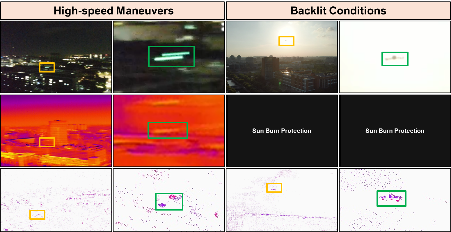
Event cameras address these limitations through asynchronous per-pixel brightness change detection with microsecond temporal resolution and high dynamic range [5]. These properties have enabled advances in remote sensing and perception tasks such as pose tracking for uncooperative spacecraft [6], visual odometry [7], space object detection [8], stereo perception [9], and single-object tracking [10]. To illustrate these advantages in A2A scenarios, Fig. 1 presents a qualitative comparison across three imaging modalities. Under high-speed maneuvers, RGB cameras produce severe motion blur that obscures the target. Under backlit conditions, thermal infrared imagery suffers from dynamic range saturation. In contrast, event cameras maintain consistent target visibility in both cases because of their unique properties. These characteristics make event cameras well-suited for A2A perception, though realizing this potential requires both representative benchmarks and efficient algorithms deployable on UAV platforms.
Existing event camera datasets for UAV perception are captured exclusively from ground-based platforms [11]–[16]. These ground-to-air configurations cannot address A2A requirements where both platforms operate in three-dimensional airspace. Such scenarios generate complex relative dynamics and dense ego-motion events across the entire field of view. Furthermore, existing annotation methods assign constant bounding boxes within inter-frame intervals, introducing systematic labeling errors during target maneuvers. To address these gaps, we introduce an Air-to-air Event-based UAV tracking dataset (AE-UAV). It is the first event camera dataset captured from an aerial platform for UAV tracking and features cubic B-spline annotations that produce \(C^2\)-continuous trajectories.
Current event-based tracking methods predominantly rely on deep neural networks [12], [17]. These methods convert events into accumulated frames and apply learned feature extractors, resulting in computational demands that are incompatible with resource-constrained UAV platforms [18]. Frequency-domain methods offer efficient alternatives through FFT-based correlation [19]–[21]. Recent work on exact Fourier transforms for event streams [22] has further demonstrated tracking feasibility. Building on these foundations, we propose a Fast-Slow Frequency-domain Tracking method (FSFT), a training-free framework tailored for A2A UAV tracking.
In this paper, we introduce a new benchmark together with a real-time tracker for A2A UAV tracking. The benchmark supports evaluation at arbitrary temporal resolutions through continuous-time annotations, and the tracker runs entirely on CPU without any training stage. The main contributions are as follows:
An air-to-air event-based UAV tracking benchmark, AE-UAV, featuring cubic B-spline continuous-time annotation. It enables the generation of \(C^2\)-continuous trajectories and supports evaluation at arbitrary temporal resolutions. To the best of our knowledge, AE-UAV is the first event-based benchmark for A2A UAV tracking.
A training-free frequency-domain tracking architecture for event streams, namely FSFT, which consists of a fast pathway that performs per-packet frequency-domain localization with Kalman prediction and a slow pathway that conducts periodic detection-based drift correction. FSFT achieves 420 FPS on CPU-only hardware without GPU dependency or training overhead.
Comprehensive experiments that validate FSFT achieving accuracy within 6.03% of state-of-the-art methods with 5.32-fold effective speedup, while revealing that deep learning trackers degrade severely at mismatched temporal resolutions whereas FSFT varies by only 6.04 percentage points.
The remainder of this paper is organized as follows. Section 2 reviews related work. Section 3 describes the AE-UAV dataset. Section 4 presents the proposed FSFT framework. Section 5 reports experimental results, ablation studies, and temporal resolution generalization analysis. Section 6 discusses the implications and limitations of this work, and Section 7 concludes the paper.
2 Related Work↩︎
This section reviews the literature most relevant to this work. Section 2.1 surveys existing event camera datasets designed for UAV tracking. Section 2.2 discusses event-based object tracking methods, covering both deep learning approaches and training-free alternatives.
2.1 Event Camera Datasets for UAV Tracking↩︎
Event camera datasets for UAV tracking have evolved from general-purpose benchmarks to specialized UAV perception datasets. General-purpose benchmarks such as VisEvent [11] and EventVOT [12] include UAV targets as minor subcategories within broader object categories. These datasets have established evaluation protocols for event-based tracking but do not focus on UAV-specific challenges. Dedicated UAV datasets have since emerged to fill this gap. F-UAV-D [13] targets indoor scenarios, while NeRDD [14] and FRED [15] extend to outdoor environments with multimodal pairing and diverse UAV types, respectively. EV-UAV [16] provides event-level annotations for 147 sequences through linear temporal extension.
As summarized in Table ¿tbl:tab:dataset95comparison?, all existing datasets capture exclusively G2A scenarios and therefore cannot model the dense ego-motion events characteristic of A2A perception, where the observer itself generates events across the entire field of view. Moreover, their annotation methods lack the continuous-time precision needed for event cameras. AE-UAV addresses both gaps with aerial-platform capture and cubic B-spline annotations that yield \(C^2\)-continuous trajectories.
| Datasets | Motion | Resolution | Target | Different | Complex | Annotation | Auxiliary | Year |
| Geometry | Illumination | Background | Method | Modality | ||||
| VisEvent [11] | G2A | 346\(\times\)260 | Generic | \(✔\) | \(\times\) | Cumulative Frame | RGB | 2023 |
| EventVOT [12] | G2A | 1280\(\times\)720 | Generic | \(✔\) | \(✔\) | Cumulative Frame | None | 2024 |
| F-UAV-D [13] | G2A | 1280\(\times\)720 | UAV | \(\times\) | \(\times\) | Cumulative Frame | RGB | 2024 |
| NeRDD [14] | G2A | 1280\(\times\)720 | UAV | \(\times\) | \(✔\) | Cumulative Frame | RGB | 2024 |
| EV-UAV [16] | G2A | 346\(\times\)240 | UAV | \(✔\) | \(✔\) | Events (Linear) | None | 2025 |
| Ev-Flying [23] | G2A | 1280\(\times\)720 | Flying | \(\times\) | \(✔\) | Cumulative Frame | None | 2025 |
| FRED [15] | G2A | 1280\(\times\)720 | UAV | \(✔\) | \(✔\) | Cumulative Frame | RGB | 2025 |
| AE-UAV | A2A | 1280\(\times\)720 | UAV | \(✔\) | \(✔\) | Cumulative Frame + | RGB + | – |
| Events (B-spline) | Thermal |
G2A = Ground-to-Air, A2A = Air-to-Air.
2.2 Event-Based Object Tracking Methods↩︎
2.2.1 Deep Learning Approaches↩︎
Recent event-based tracking methods predominantly rely on deep neural networks that convert event streams into accumulated frames for feature extraction. EventVOT [12] establishes state-of-the-art benchmarks for high-resolution event tracking through transformer-based architectures. MambaEVT [17] introduces efficient sequential modeling via the Mamba architecture for event temporal dynamics. General-purpose trackers such as OSTrack [24], ARTrack [25], ROMTrack [26], AQATrack [27], and ODTrack [28] achieve competitive results when adapted to event data through frame reconstruction.
These methods face two limitations for A2A UAV tracking. First, their GPU requirements are incompatible with resource-constrained aerial platforms [18]. Second, event-to-frame conversion discards microsecond temporal resolution and introduces processing latency. Although efficient architectures [29] and neuromorphic computing [30] have begun to address these issues, a lightweight event-native solution for A2A tracking remains absent.
2.2.2 Training-Free Approaches↩︎
Training-free methods preserve event-native characteristics without labeled data. Time surface representations [31] encode event recency through exponential decay kernels, enabling efficient pattern matching. Optical flow methods [32] compute per-pixel motion vectors from spatiotemporal event distributions for target displacement recovery. Asynchronous corner detection [33] and photometric feature tracking [34] exploit event-intrinsic properties to achieve robust asynchronous feature tracking and motion estimation.
Frequency-domain methods offer particular advantages for efficient tracking. KCF [19] achieves high-speed tracking through circulant matrix decomposition. DCF [20] and ECO [21] extend this with spatial reliability and efficient convolution operators, respectively. The eFFT framework [22] further demonstrates exact Fourier transform computation directly from asynchronous event streams.
Our FSFT combines frequency-domain template matching with event-intrinsic features. The per-packet localization employs Fourier magnitude spectrum correlation for rapid target positioning. The periodic correction exploits event-native cues to detect and correct drift before it accumulates.
3 AE-UAV Dataset↩︎
This section describes the AE-UAV dataset in detail. Section 3.1 introduces the acquisition system and collection plan. Section 3.2 presents the continuous-time annotation framework based on cubic B-spline interpolation. Section 3.3 summarizes the dataset statistics and partitioning strategy.
3.1 Acquisition System and Plan↩︎
The acquisition system employs two coordinated UAVs for systematic capture of realistic aerial scenarios. The observer platform is a DJI Matrice 300 RTK carrying a Prophesee EVK4 HD event camera with \(1280 \times 720\) resolution and a 12 mm fixed-focus lens. A DJI Zenmuse H20T gimbal provides auxiliary imagery via an RGB camera with 1920\(\times\)1080 resolution and a thermal infrared camera with 640\(\times\)512 resolution. In addition, an onboard inertial measurement unit (IMU) records six-axis motion data at 200 Hz. The target is a DJI Mavic 3T that is representative of typical small UAVs in surveillance and counter-UAV applications. Fig. 2 (a) illustrates the system configuration.
The acquisition plan systematically varies scenarios along multiple dimensions, as summarized in Table 1. Backgrounds range from textured urban areas to clear sky. Illumination spans normal daylight, backlit, and nighttime conditions. Three relative motion patterns are captured as shown in Fig. 2 (b): evasion, pursuit, and head-on approach. Target trajectories encompass straight-line, turning, lateral, and vertical maneuvers. The inter-UAV distance ranges from 15 to 100 m, producing target scales from point-like signatures to detailed structures.

| Factor | Category | Sequences |
|---|---|---|
| Motion Geometry | Pursuit | 78 |
| Evasion | 81 | |
| Head-on Approach | 19 | |
| Illumination | Normal Daylight | 29 |
| Backlit | 10 | |
| Night with Target Lights On | 98 | |
| Night with Target Lights Off | 41 | |
| Trajectory | Straight-line | 27 |
| Turning | 89 | |
| Lateral Maneuver | 42 | |
| Vertical Maneuver | 20 |
3.2 Continuous-Time Annotation↩︎
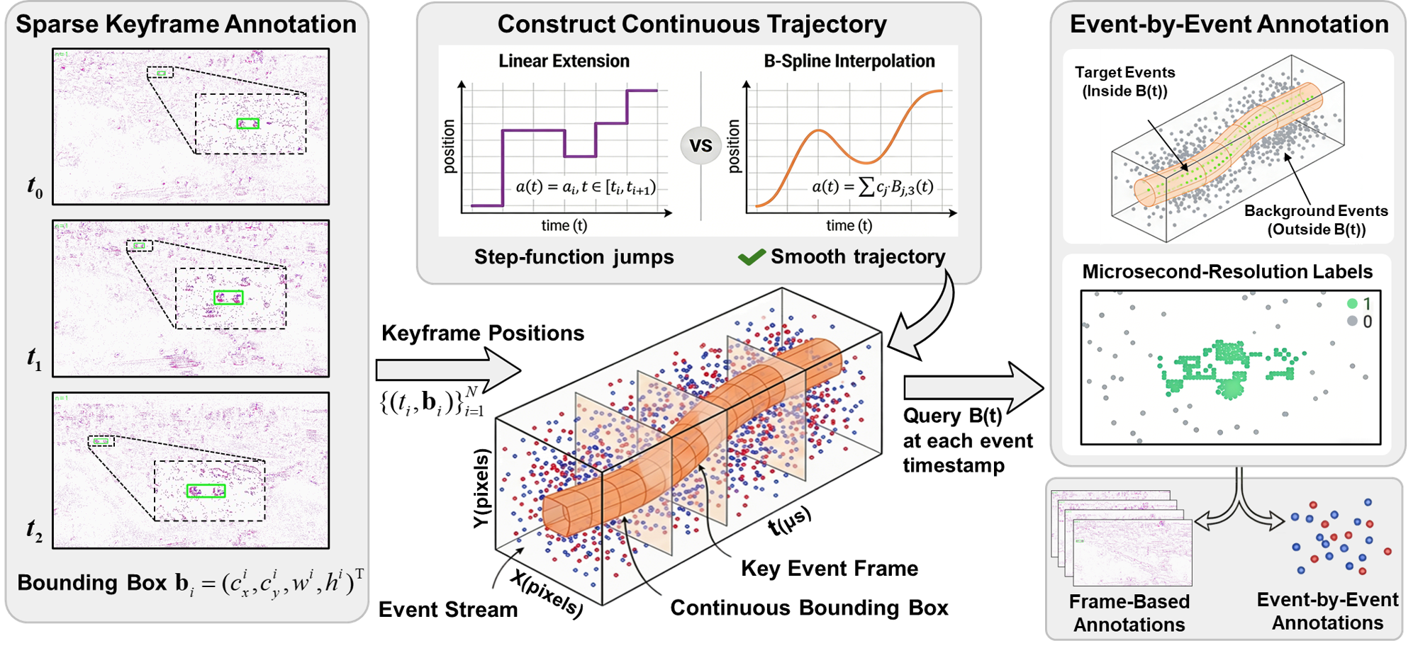
Conventional annotation methods assign constant bounding boxes within inter-frame intervals, creating a mismatch between the continuous nature of event streams and the discrete nature of ground truth labels. In event-based tracking, this mismatch is particularly problematic because events are generated asynchronously at microsecond resolution, and a target can move significantly between two consecutive keyframes. When evaluating trackers at different temporal resolutions, constant bounding box labels produce inconsistent ground truth, making fair cross-resolution comparison impossible. A continuous annotation framework is therefore essential for event-based benchmarks that aim to support evaluation across varying temporal scales.
We propose a continuous-time annotation framework based on cubic B-spline interpolation that bridges sparse keyframe annotations and dense event-level labels. This framework offers two practical advantages. First, it enables consistent evaluation at arbitrary temporal resolutions from a single annotation effort, greatly reducing the total annotation cost. Second, it produces physically plausible trajectories with smooth position, velocity, and acceleration profiles, ensuring that the ground truth reflects realistic target dynamics rather than artificial step-function jumps.
The pipeline operates in three stages as illustrated in Fig. 3. First, human annotators label bounding boxes on accumulated event frames at sparse keyframe timestamps, yielding \(N\) observations \(\{(t_i, \mathbf{b}_i)\}_{i=1}^{N}\) where \(\mathbf{b}_i = (c_x^i, c_y^i, w^i, h^i)^\top\). Second, a continuous trajectory is constructed via B-spline interpolation. Third, each event is assigned a binary label by querying this trajectory.
Prior work such as EV-UAV [16] employs linear temporal extension: \[\mathbf{B}_{\mathrm{linear}}(t) = \mathbf{b}_i, \quad \text{for } t \in [t_i, t_{i+1}) \label{eq:linear}\tag{1}\] This piecewise constant approximation assumes zero intra-frame motion. Such an assumption is frequently violated during maneuvers where target position evolves nonlinearly between keyframes.
We model each bounding box parameter \(a \in \{c_x, c_y, w, h\}\) as a cubic B-spline curve: \[a(t) = \sum_{j=0}^{M-1} c_j B_{j,3}(t) \label{eq:bspline}\tag{2}\] where \(M\) is the number of control points, \(c_j\) denotes the \(j\)-th coefficient, and \(B_{j,3}(t)\) is the cubic B-spline basis function that guarantees \(C^2\) continuity. This formulation ensures smooth position, velocity, and acceleration profiles that correspond to physically plausible target dynamics. The control points are computed via regularized least-squares: \[{!}{\begin{align} \{c_j^*\} = \arg\min_{\{c_j\}} \left[ \sum_{i=1}^{N} \left\| a(t_i) - a_i \right\|^2 + \lambda \int_{t_1}^{t_N} \left\| \ddot{a}(t) \right\|^2 \, dt \right] \label{eq:optimization} \end{align}}\tag{3}\] where the first term enforces interpolation fidelity, the second penalizes excessive curvature to prevent overfitting, and \(\lambda = 0.001\).
Given the fitted trajectory \(\mathbf{B}(t) = (c_x(t), c_y(t), w(t), h(t))\), each event \(e_k = (x_k, y_k, t_k, p_k)\) is assigned a binary label: \[\ell_k = \begin{cases} 1, & \text{if } (x_k, y_k) \in \mathcal{R}\bigl(\mathbf{B}(t_k)\bigr) \\ 0, & \text{otherwise} \end{cases} \label{eq:event95label}\tag{4}\] where \(\mathcal{R}(\mathbf{B}(t))\) denotes the rectangular region defined by \(\mathbf{B}(t)\). The pipeline produces dual output formats, namely frame-level annotations for conventional trackers and event-level labels for methods operating at native temporal resolution.
3.3 Dataset Statistics and Partitioning↩︎
The AE-UAV dataset comprises 178 sequences totaling approximately 2,140 seconds and over 8.15 billion events, of which 31.2 million are target events accounting for 0.38% of all events. This extreme class imbalance is inherent in A2A scenarios where the target subtends a small portion of the field of view. Fig. 4 provides a qualitative overview of the dataset across representative scenes. Each column corresponds to a different scene, which together cover urban skylines, low light night flights, and cluttered backgrounds. This visualization highlights the dense ego-motion events that fill the field of view and the small spatial footprint of the target relative to the surrounding clutter.
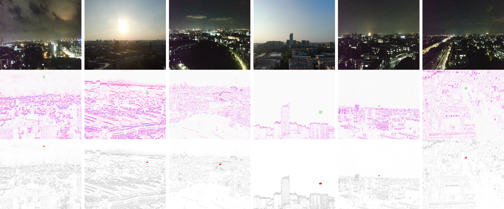
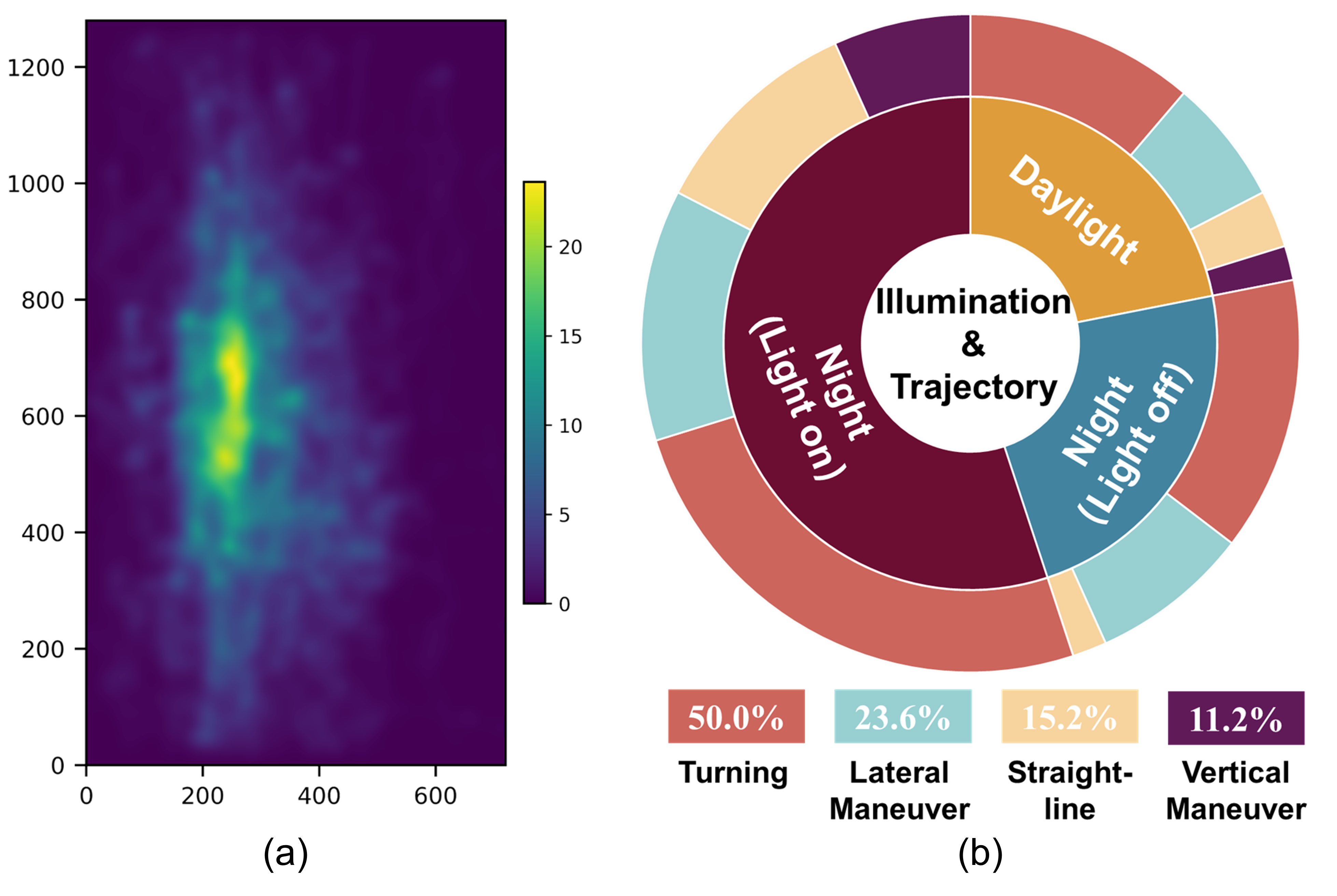
Fig. 5 (a) shows the spatial distribution of target centers, which predominantly appear in the central and upper regions. Small targets in \([16^2, 32^2)\) pixels constitute 57.3% and medium targets in \([32^2, 64^2)\) pixels account for 40.1%. The remaining 2.6% comprises tiny and large targets. Fig. 5 (b) presents the joint distribution of trajectory patterns and illumination. The dataset emphasizes nighttime sequences to reflect real-world counter-UAV surveillance requirements in A2A operations. Turning maneuvers are the most frequent trajectory pattern across all conditions, followed by lateral and vertical maneuvers.
The dataset is partitioned into training, validation, and test subsets containing 125, 18, and 35 sequences, respectively. Two-level hierarchical stratified sampling based on motion geometry and target scale ensures balanced representation, with each subset containing sequences from all major scenario categories. The training set is provided for methods that require supervised learning, while the test set is reserved for final evaluation to prevent overfitting.
4 Proposed Method↩︎
This section presents the FSFT framework. Section 4.1 provides the system overview and overall design rationale. Section 4.2 details the fast pathway that performs per-packet frequency-domain localization. Section 4.3 describes the slow pathway that conducts periodic detection-based correction.
4.1 System Overview↩︎
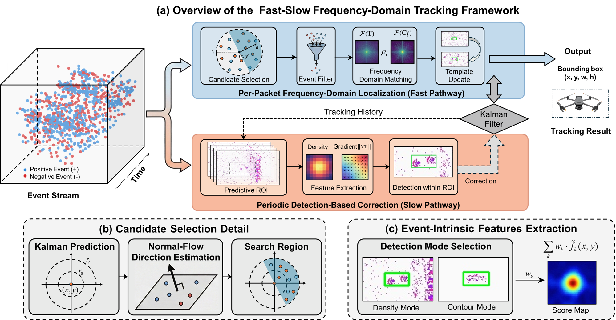
The AE-UAV dataset reveals three requirements for A2A event-based tracking that expose the limitations of existing methods. First, small UAV platforms preclude dedicated GPUs while current deep learning trackers rely on GPU acceleration. Second, A2A scenarios demand high temporal resolution but event-to-frame conversion discards fine-grained timing. Third, dense ego-motion events create a low signal-to-noise environment where target events account for only 0.38% of all events. These observations motivate three core design principles for FSFT. First, the framework processes event packets directly without constructing dense frames. Second, it runs in real time on CPU-only hardware with no training overhead. Third, it employs frequency-domain representations that naturally encode edge structure at characteristic frequencies and attenuate spatially incoherent noise.
As illustrated in Fig. 6, the fast pathway performs per-packet frequency-domain localization via Kalman prediction, normal-flow direction estimation, and template matching. The slow pathway activates every \(N\) packets for detection-based drift correction within a predicted region of interest. The two pathways interact bidirectionally. Localization estimates define regions of interest (ROI) for periodic detection, while validated detections reset the localization state. Both pathways share a unified Kalman filter state.
4.2 Per-Packet Frequency-Domain Localization↩︎
This subsection details the fast pathway of FSFT, which runs on every incoming event packet and produces a target location estimate at sub-millisecond latency through candidate selection and frequency-domain template matching.
4.2.1 Candidate Selection↩︎
4.2.1.1 Kalman Prediction with Adaptive Search Radius.
We model target dynamics using a constant-velocity Kalman filter [35] with state \(\mathbf{x}_t = [x, y, \dot{x}, \dot{y}]^\top\): \[\hat{\mathbf{x}}_{t|t-1} = \mathbf{F} \mathbf{x}_{t-1|t-1}, \quad \mathbf{P}_{t|t-1} = \mathbf{F} \mathbf{P}_{t-1|t-1} \mathbf{F}^\top + \mathbf{Q} \label{eq:kalman95predict}\tag{5}\] where \(\mathbf{F}\) is the state transition matrix and \(\mathbf{Q}\) is the process noise covariance. The search radius adapts based on prediction uncertainty: \[r_t = r_0 + \alpha \cdot \text{tr}(\mathbf{P}_{t|t-1}^{xy}) \label{eq:adaptive95radius}\tag{6}\] where \(\mathbf{P}^{xy}\) is the position covariance submatrix. This mechanism expands the search region under unpredictable motion and constrains it under stable tracking, improving both robustness and efficiency.
4.2.1.2 Normal Flow-based Direction Estimation.
Normal flow represents the motion component perpendicular to local edge orientation, which is directly observable from events [36]. Given events \(\{(x_i, y_i, t_i)\}_{i=1}^{n}\) within a spatial window, the direction is estimated by fitting a local spatiotemporal plane: \[\min_{a, b, c} \sum_{i=1}^{n} (t_i - ax_i - by_i - c)^2 \label{eq:plane95fitting}\tag{7}\] yielding the normalized direction vector: \[\mathbf{d} = \frac{1}{\sqrt{a^2 + b^2}} \begin{bmatrix} a \\ b \end{bmatrix} \label{eq:normal95flow95dir}\tag{8}\] This formulation exploits the geometric relationship between event timing and edge motion. Pixels traversed earlier by a moving edge have smaller timestamps, and the gradient of the fitted plane points in the motion direction.
4.2.1.3 Direction-Guided Candidate Generation.
Given predicted position \(\hat{\mathbf{p}}_t\), adaptive radius \(r_t\), and direction \(\mathbf{d}_t\), candidates are generated within a forward-facing angular sector: \[\mathcal{C}_t = \left\{\hat{\mathbf{p}}_t + \boldsymbol{\delta} : \|\boldsymbol{\delta}\| \leq r_t, \; \frac{\boldsymbol{\delta} \cdot \mathbf{d}_t}{\|\boldsymbol{\delta}\|} \geq \cos\theta \right\} \label{eq:candidate95cone}\tag{9}\] where \(\theta\) is the cone half-angle. This reduces the search area by approximately 50% while focusing resources on probable target locations.
4.2.2 Frequency-Domain Template Matching↩︎
4.2.2.1 Event Filtering.
Event cameras generate high-bandwidth asynchronous data streams that inherently contain substantial redundancy. Following the eFFT framework [22], we implement two complementary filtering mechanisms to reduce computational load while preserving tracking-relevant information.
First, repeated event removal retains only the most recent event at each pixel per packet. This effectively removes redundant triggers that do not contribute additional spatial information for template matching. Second, reactivated event filtering identifies and excludes events that both enter and exit the sliding temporal window at the same pixel: \[\mathcal{E}_{\mathrm{react}} = \left\{e \in \mathcal{E}_{\mathrm{in}} : \exists\, e' \in \mathcal{E}_{\mathrm{out}},\; (x_e, y_e) = (x_{e'}, y_{e'})\right\} \label{eq:reactivated}\tag{10}\] where \(\mathcal{E}_{\mathrm{in}}\) and \(\mathcal{E}_{\mathrm{out}}\) denote the sets of incoming and outgoing events, respectively. These reactivated events typically correspond to static edges or sensor noise rather than target motion and are therefore excluded from processing.
4.2.2.2 Magnitude Spectrum Correlation.
Template matching uses normalized cross-correlation on Fourier magnitude spectra. Given the template spectrum \(|\mathcal{F}(\mathbf{T})|\) and a candidate spectrum \(|\mathcal{F}(\mathbf{C}_i)|\), the similarity is computed as: \[\rho_i = \frac{\langle |\mathcal{F}(\mathbf{T})| - \mu_T,\; |\mathcal{F}(\mathbf{C}_i)| - \mu_i \rangle}{\sigma_T \cdot \sigma_i} \label{eq:ncc}\tag{11}\] where \(\mu\) and \(\sigma\) denote the mean and standard deviation of the respective spectra. The candidate with the highest \(\rho^* = \max_i \rho_i\) is selected as the tracking output, provided it exceeds the threshold \(\tau_{\text{match}}\). This approach offers three key advantages. First, the magnitude spectrum is shift-invariant, providing robustness to small localization errors. Second, FFT-based correlation achieves \(O(n \log n)\) complexity, enabling CPU-only real-time processing. Third, edge information concentrates at characteristic frequencies, naturally attenuating high-frequency sensor noise.
4.2.3 Adaptive Template Update↩︎
A confidence-gated exponential moving average prevents template corruption during challenging conditions: \[\mathbf{T}_{t} = \begin{cases} (1 - \eta) \mathbf{T}_{t-1} + \eta \, \mathbf{C}_{\text{best}} & \text{if } \rho^* > \tau_{\text{conf}} \\[2pt] \mathbf{T}_{t-1} & \text{otherwise} \end{cases} \label{eq:template95update}\tag{12}\] where \(\eta \in (0, 1)\) is the learning rate and \(\mathbf{C}_{\text{best}}\) is the event representation at the best-matching position. The template evolves only under high-confidence matches, maintaining integrity during occlusions or temporary target absence.
4.3 Periodic Detection-Based Correction↩︎
Frequency-domain template matching is highly efficient but it is sensitive to long-term appearance drift. To address this issue, we introduce a complementary slow pathway that operates at a lower temporal rate and refines the estimate produced by the fast pathway. This subsection details the slow pathway of FSFT, which activates every \(N\) event packets to correct drift and adapt target scale through local detection.
4.3.1 Predictive Region of Interest↩︎
Rather than searching the entire field of view, detection is constrained to a predictive ROI extrapolated from recent localization positions via linear extrapolation. This ROI-based processing reduces computational complexity by limiting feature extraction to a small fraction of the image area. It also suppresses background noise interference by excluding regions with spurious non-target events.
4.3.2 Event-Intrinsic Feature Extraction↩︎
Within the ROI, two features are extracted to exploit the intrinsic characteristics of event camera data for target detection.
The first characteristic is event density. Moving objects generate concentrated event clusters as their surfaces continuously trigger events across the pixel array [37]. The event density map \(D(x,y)\) is obtained by accumulating events at each pixel location and applying Gaussian smoothing: \[D(x,y) = G_\sigma * \sum_{k} \mathbf{1}\bigl[(x_k, y_k) = (x, y)\bigr] \label{eq:density}\tag{13}\] where \(G_\sigma\) denotes a Gaussian kernel with bandwidth \(\sigma\) and \(\mathbf{1}[\cdot]\) is the indicator function. Regions with abnormally high density indicate potential target locations where coherent motion produces sustained event generation.
The second characteristic is gradient magnitude. The time surface \(\mathbf{S}(x,y)\) [38] records the most recent event timestamp at each pixel, weighted by an exponential decay kernel. Its gradient magnitude is computed via the Scharr operator as \[\|\nabla \mathbf{S}(x,y)\| = \sqrt{\left(\frac{\partial \mathbf{S}}{\partial x}\right)^2 + \left(\frac{\partial \mathbf{S}}{\partial y}\right)^2} \label{eq:gradient}\tag{14}\] High gradient magnitude corresponds to edges in motion, a characteristic signature of rigid body translation against the background. Background noise events, by contrast, produce spatially incoherent gradients that are naturally attenuated by this measure. These two features capture complementary aspects of the target signature. Event density reflects the spatial energy concentration of moving targets, while gradient magnitude encodes boundary structure at higher spatial frequencies.
4.3.3 Weighted Feature Fusion↩︎
To accommodate diverse illumination conditions, the detection mode is automatically selected based on initial template characteristics.
Density Mode is used for nighttime scenes with target light on, where targets produce high-contrast event bursts with concentrated spatial distributions. In addition to event density \(D\) and gradient magnitude \(\|\nabla \mathbf{S}\|\), this mode computes two supplementary features derived from these primary representations.
Direction consistency quantifies the local alignment of time surface gradients. Let \(d_x = (\partial \mathbf{S}/\partial x) / \|\nabla \mathbf{S}\|\) and \(d_y = (\partial \mathbf{S}/\partial y) / \|\nabla \mathbf{S}\|\) denote the unit gradient direction at each pixel. The consistency is computed through local averaging weighted by a gradient confidence mask \(\mathbf{m}(x,y) = \mathbf{1}[\|\nabla \mathbf{S}\| > \tau_g]\): \[\Gamma(x,y) = \sqrt{\bigl(\overline{d_x \cdot \mathbf{m}}\bigr)^2 + \bigl(\overline{d_y \cdot \mathbf{m}}\bigr)^2} \label{eq:direction95consistency}\tag{15}\] where \(\overline{(\cdot)}\) denotes local averaging within a \(W \times W\) window. A high \(\Gamma\) indicates coherent motion direction expected for a rigid target, while random background noise yields low \(\Gamma\) due to incoherent gradient orientations.
Spatial compactness evaluates how tightly events are grouped around local density peaks, defined as the ratio between the smoothed density and the local maximum density: \[\Phi(x,y) = \frac{D(x,y)}{\max_{(u,v) \in \mathcal{N}(x,y)} D(u,v) + \epsilon} \label{eq:spatial95compactness}\tag{16}\] where \(\mathcal{N}(x,y)\) is a rectangular neighborhood and \(\epsilon\) is a small constant for numerical stability. A value close to unity indicates a compact event cluster typical of illuminated targets. The density mode assigns the highest weight to event density, followed by direction consistency, spatial compactness, and gradient magnitude.
Contour Mode is used for daytime scenes or nighttime scenes with target light off, where targets generate sparser events primarily along their silhouette boundaries. Beyond the two primary features, this mode computes two supplementary features that build upon the time surface \(\mathbf{S}\) and enhance sensitivity to elongated edge structures.
Edge density measures the local concentration of detected edge pixels. Adaptive Canny edge detection is applied to the time surface, and the resulting binary edge map is smoothed to obtain a continuous density: \[\mathcal{D}_e(x,y) = G_{\sigma_e} * \mathbf{E}(x,y), \quad \mathbf{E} = \mathrm{Canny}\!\bigl(\mathbf{S},\; \tau_l,\; \tau_h\bigr) \label{eq:edge95density}\tag{17}\] where \(\tau_l\) and \(\tau_h\) are adaptive thresholds derived from the median intensity of the time surface and \(\sigma_e\) is the smoothing bandwidth.
Contour coherence evaluates whether the detected edges form continuous boundary segments. A morphological skeleton \(\mathbf{K}\) is extracted from the binarized time surface, and the connectivity of each skeleton pixel is measured by counting its eight-connected neighbors \(n_{\mathrm{nb}}\): \[\Psi(x,y) = \exp\!\bigl(-\lambda_c \,|n_{\mathrm{nb}}(x,y) - 2|\bigr) \cdot \mathbf{K}(x,y) \label{eq:contour95coherence}\tag{18}\] where \(\lambda_c\) is a decay parameter. A skeleton pixel with exactly two neighbors lies along a continuous contour and yields the maximum coherence. This feature distinguishes coherent silhouettes from scattered noise edges. The contour mode assigns the highest weight to edge density, followed by contour coherence, gradient magnitude, and event density.
The selected features are combined through weighted summation: \[S(x, y) = \frac{\sum_{k} w_k \cdot \tilde{f}_k(x, y)}{\sum_{k} w_k} \label{eq:select}\tag{19}\] where \(\tilde{f}_k\) is the min-max normalized feature map and \(w_k\) is the weight determined by the detection mode. The score map is adaptively thresholded based on its percentile distribution, followed by morphological operations and connected component analysis to extract candidate bounding boxes. Valid detections, identified through aspect ratio and compactness constraints, reset the Kalman filter state and update the target scale.
5 Experiments↩︎
This section presents the experimental evaluation of the proposed approach. Section 5.1 describes the experimental setup and evaluation metrics. Section 5.2 compares FSFT with state-of-the-art tracking methods. Section 5.3 analyzes scenario-specific performance. Section 5.4 reports ablation studies. Section 5.5 evaluates temporal resolution generalization.
5.1 Experimental Setup↩︎
All experiments are conducted on a workstation with an Intel Core i5-12400F CPU and an NVIDIA GeForce RTX 3090 GPU. Deep learning baselines use official implementations trained on the 125-sequence training subset. Each method is evaluated at the event accumulation frequency that yields its best accuracy. The accumulation frequency determines the temporal duration of each event packet. For example, 30 Hz corresponds to a packet duration of 33.3 ms.
Three accuracy metrics are adopted. Success Rate AUC (SR-AUC) measures the area under the success plot across IoU thresholds [39]. Precision Rate (PR) at 20 pixels counts frames where center error falls below 20 pixels [39]. Normalized Precision Rate (NPR) at 0.2 provides scale-normalized precision [40]. Two throughput metrics are also reported. Test FPS measures the inference speed of each method, where event frame-based methods directly process pre-rendered accumulated frames. Actual FPS measures the end-to-end throughput from receiving raw event data to producing the final tracking output, which additionally includes the event-to-frame rendering time.
To jointly evaluate accuracy and throughput, we further report a supplementary A2A Tracking Quality metric, defined as \(\text{ATQ} = \text{SR-AUC} \times \log_{30}(\text{Actual FPS})\). We adopt 30 FPS as the reference rate because it is the minimum throughput for smooth real-time tracking on deployed platforms, so that a method operating at this rate receives a neutral scaling factor of unity. Following the VOT protocol [41] and large-scale benchmarks [42] that couple accuracy with processing speed, the logarithmic scaling reflects the diminishing marginal benefit of higher frame rates and penalizes methods that are accurate but too slow for onboard deployment. ATQ is intended as a relative summary of the accuracy–throughput trade-off among real-time-capable trackers rather than an absolute quality score; the standard metrics (SR-AUC, PR, NPR) remain the primary basis for comparison.
| Method | Source | Event Rep | SR-AUC\(\uparrow\) | PR\(\uparrow\) | NPR\(\uparrow\) | |||||
| FPS\(\uparrow\) | ||||||||||
| FPS\(\uparrow\) | ATQ | Platform | Training | |||||||
| OSTrack [24] | ECCV22 | Event Frame | 32.95 | 59.20 | 38.67 | 148 | 89 | 43.48 | GPU | Req. |
| SimTrack [43] | ECCV22 | Event Frame | 32.89 | 58.89 | 39.05 | 46 | 38 | 35.18 | GPU | Req. |
| ARTrack [25] | CVPR23 | Event Frame | 47.15 | 71.25 | 62.95 | 24 | 22 | 42.85 | GPU | Req. |
| ROMTrack [26] | ICCV23 | Event Frame | 55.82 | 86.84 | 75.32 | 126 | 80 | 71.92 | GPU | Req. |
| AQATrack [27] | CVPR24 | Event Frame | 56.07 | 88.52 | 80.23 | 112 | 74 | 70.95 | GPU | Req. |
| ODTrack [28] | AAAI24 | Event Frame | 35.24 | 64.25 | 42.68 | 30 | 26 | 33.76 | GPU | Req. |
| MambaEVT [17] | TCSVT25 | Event Frame | 40.56 | 65.38 | 40.68 | 20 | 18 | 34.47 | GPU | Req. |
| FocusTrack [2] | TGRS25 | Event Frame | 60.05 | 88.37 | 81.63 | 122 | 79 | 77.14 | GPU | Req. |
| FSFT | – | Event Packet | 56.43 | 88.45 | 79.49 | 420 | 420 | 100.22 | CPU | Free |
Req. = Required. Bold indicates best; underline indicates second best.
5.2 Overall Performance Comparison↩︎
Table ¿tbl:tab:contrast? presents the quantitative comparison. Deep learning methods achieve optimal performance at 30 Hz, while FSFT performs best at 60 Hz. Among deep learning trackers, FocusTrack [2] achieves the highest SR-AUC of 60.05% while AQATrack [27] attains the best PR of 88.52%. FSFT achieves 56.43% SR-AUC with PR of 88.45%, representing 93.97% of FocusTrack’s accuracy while operating at 420 FPS on CPU-only hardware without any training.
The gap between Test FPS and Actual FPS highlights deployment implications. ROMTrack and FocusTrack reach 126 and 122 FPS for inference alone, but the event-to-frame rendering overhead reduces their actual throughput to 80 and 79 FPS. In contrast, FSFT operates directly on event packets at 420 FPS, yielding a 5.32-fold effective speedup over FocusTrack with substantially lower power consumption. On the ATQ metric, FSFT achieves 100.22, leading the second-best FocusTrack by an absolute margin of 23.08 percentage points. For A2A UAV tracking where onboard computational efficiency is a primary constraint, FSFT provides an efficient standalone solution with immediate deployment capability.
| Metric | Method | Target Characteristics | Complex | Motion Geometry | ||||
|---|---|---|---|---|---|---|---|---|
| 3-5 (lr)7-9 | Small | Scale | Direction | Background | Pursuit | Evasion | Head-on | |
| OSTrack [24] | 28.30 | 26.76 | 24.26 | 20.15 | 22.64 | 43.54 | 21.94 | |
| ROMTrack [26] | 52.68 | 49.49 | 51.69 | 49.83 | 55.26 | 59.19 | 43.72 | |
| AQATrack [27] | 54.03 | 53.34 | 55.96 | 50.52 | 55.42 | 59.51 | 44.11 | |
| MambaEVT [17] | 38.72 | 35.43 | 38.18 | 34.47 | 36.76 | 47.63 | 26.02 | |
| FocusTrack [2] | 56.55 | 55.37 | 58.33 | 54.95 | 60.97 | 62.13 | 47.45 | |
| FSFT | 54.41 | 55.63 | 56.05 | 51.11 | 56.30 | 58.52 | 48.03 | |
| OSTrack [24] | 37.35 | 35.32 | 32.02 | 26.59 | 29.88 | 57.46 | 28.95 | |
| ROMTrack [26] | 67.87 | 63.76 | 66.60 | 64.20 | 71.20 | 76.26 | 56.33 | |
| AQATrack [27] | 68.37 | 67.50 | 70.81 | 63.93 | 70.13 | 75.31 | 55.82 | |
| MambaEVT [17] | 32.90 | 30.11 | 32.45 | 29.29 | 31.24 | 40.48 | 22.11 | |
| FocusTrack [2] | 72.65 | 71.13 | 74.94 | 70.59 | 78.33 | 79.82 | 60.96 | |
| FSFT | 96.63 | 98.79 | 99.54 | 90.77 | 99.98 | 103.93 | 85.30 | |
Small = Small target; Scale = Scale variation; Direction = Direction change.
5.3 Scenario-Specific Performance Analysis↩︎
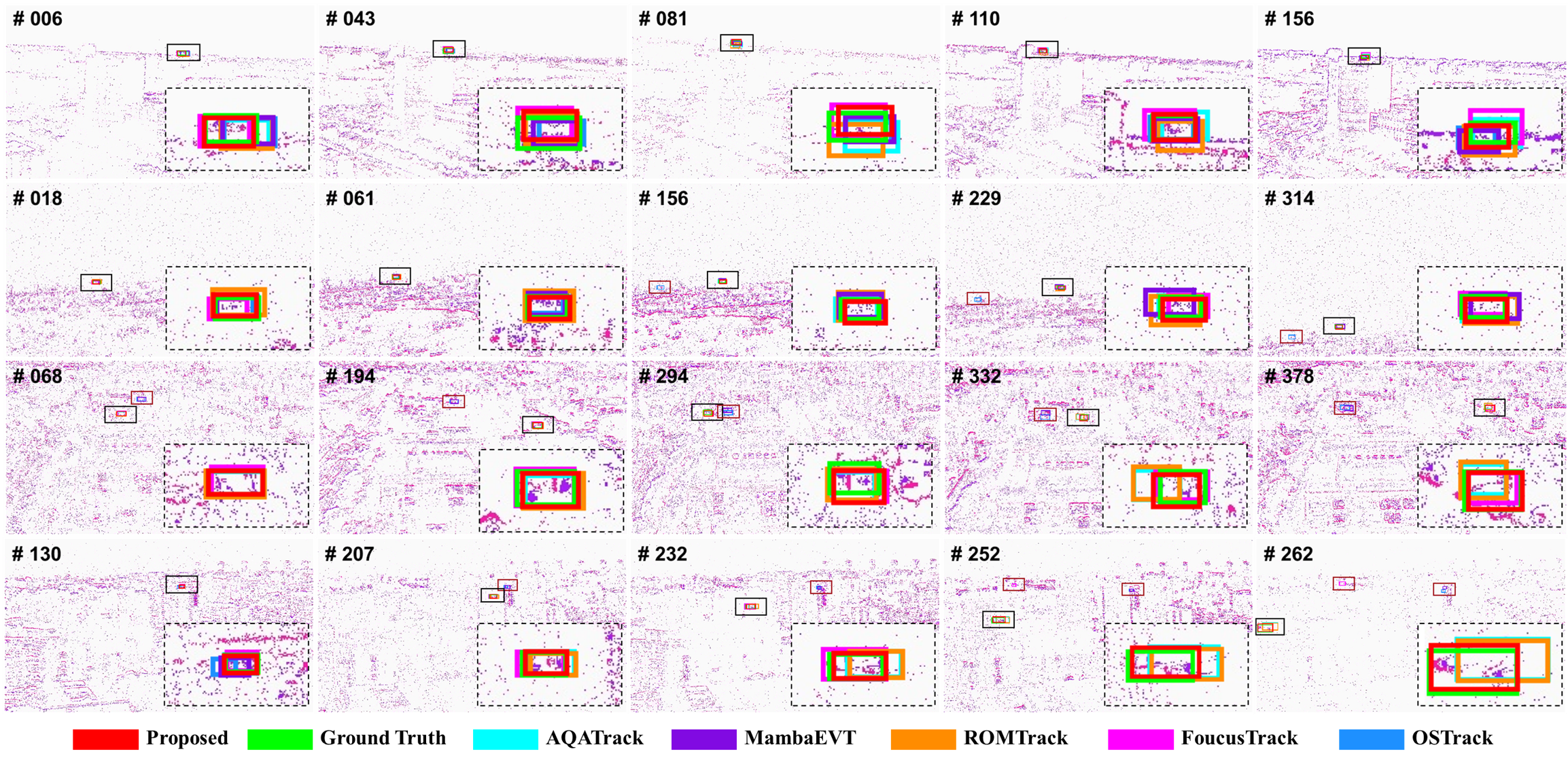
Table ¿tbl:tab:performance95conditions? presents scenario-specific SR-AUC and ATQ results. Fig. 7 provides qualitative visualization. Under scale variation, FSFT achieves the best SR-AUC of 55.63%, benefiting from shift-invariance of the Fourier magnitude spectrum and confidence-gated template update. Under direction changes, FSFT achieves 56.05%, validating Kalman prediction and normal flow estimation. For background complexity, FSFT reaches 51.11% versus FocusTrack’s 54.95%, a gap of 3.84 percentage points, as high-frequency clutter interferes with FFT-based matching. For head-on approach, FSFT achieves the best SR-AUC of 48.03% among all methods. On the trade-off summarized by ATQ, FSFT’s large throughput advantage consistently outweighs its accuracy gap relative to deep learning methods across all seven scenario categories.
5.4 Ablation Study↩︎
Table 2 quantifies the contribution of each component. Each ablation variant disables only the designated component while all other components remain fully active. The Origin configuration applies minimal FFT matching without any of the three proposed components, achieving only 21.34% SR-AUC. This result shows that naive frequency-domain matching alone is insufficient for robust tracking.
The variant without detection-based correction suffers the largest degradation, dropping to 31.62% SR-AUC, a decline of 24.81 percentage points relative to the full system. This result validates that periodic drift correction is the most critical component for long-term tracking stability. The variant without Kalman filtering reduces performance to 45.13%, which confirms that constraining the search space through state prediction is essential under dynamic target motion. The variant without direction estimation yields 53.62% SR-AUC, which demonstrates that normal-flow pruning provides measurable precision gains in addition to its computational savings.
The full system maintains 420 FPS. Detection-based correction contributes 1.1 ms per activation, Kalman prediction adds 0.1 ms per packet, and direction estimation adds 0.06 ms per packet. The throughput reduction from 780 to 420 FPS reflects the computational overhead of the correction pathway, which is well justified by the 24.81-point SR-AUC improvement.
| Configuration | SR-AUC\(\uparrow\) | PR\(\uparrow\) | NPR\(\uparrow\) | FPS\(\uparrow\) | Latency |
|---|---|---|---|---|---|
| Origin | 21.34 | 45.85 | 35.66 | 1200 | – |
| FSFT | 56.43 | 88.45 | 79.49 | 420 | – |
| w/o Correction | 31.62 | 55.51 | 44.26 | 780 | 1.1ms |
| w/o Kalman | 45.13 | 70.83 | 62.49 | 439 | 0.1ms |
| w/o Direction | 53.62 | 85.32 | 70.95 | 392 | 0.06ms |
5.5 Temporal Resolution Generalization↩︎
Table ¿tbl:tab:temporal? evaluates performance across different temporal resolutions. Deep learning methods exhibit substantial degradation when tested at resolutions differing from their training frequency. ROMTrack trained at 30 Hz drops from 55.82% to 0.52% at 200 Hz. AQATrack trained at 30 Hz shows a similar collapse from 56.07% to 0.98% at 200 Hz. FocusTrack trained at 30 Hz drops from 60.05% to 3.40% at 200 Hz. This degradation occurs because networks learn features specific to temporal aggregation patterns that become invalid at different event densities. Higher-frequency training improves generalization. For example, FocusTrack trained at 60 Hz maintains 48.32% at 200 Hz and achieves the best average of 53.28% among all deep learning configurations. AQATrack trained at 60 Hz follows a similar trend with an average of 44.48%.
FSFT maintains stable performance across all resolutions, ranging from 50.39% to 56.43% with a maximum variation of 6.04 percentage points. This stability benefits from the training-free design that eliminates temporal pattern dependency and from the frequency-domain robustness to event density variations. FSFT achieves the highest average SR-AUC of 53.62% across all resolutions, slightly surpassing the best deep learning configuration. The continuous-time annotations of AE-UAV enable this evaluation by providing ground truth at arbitrary resolutions without systematic labeling errors.
llccccc & 200 Hz & 120 Hz & 60 Hz & 30 Hz & Average
& 50.39 & 56.43 & 55.85 & 51.84 & 53.62
& ROMTrack & 0.52 & 1.85 & 3.71 & 55.82 & 15.48
& AQATrack & 0.98 & 1.76 & 3.41 & 56.07 & 15.56
& FocusTrack & 3.40 & 6.41 & 7.01 & 60.05 & 19.22
& ROMTrack & 38.41 & 40.26 & 53.97 & 49.58 & 45.56
& AQATrack & 38.27 & 39.51 & 54.63 & 45.51 & 44.48
& FocusTrack & 48.32 & 51.57 & 59.53 & 53.71 & 53.28
& ROMTrack & 29.06 & 38.43 & 48.57 & 49.08 & 41.29
& AQATrack & 25.33 & 39.87 & 45.35 & 48.63 & 39.80
& FocusTrack & 28.38 & 42.97 & 48.43 & 46.61 & 41.60
6 Discussion↩︎
The experimental results validate both primary contributions. The AE-UAV dataset fills a critical gap by providing realistic A2A motion patterns. In particular, head-on encounters stress-test existing methods and reveal performance characteristics that cannot be observed on ground-based benchmarks. FSFT further demonstrates that competitive accuracy is achievable on CPU hardware without any training stage, which makes real-time deployment on small UAV platforms feasible. The temporal resolution experiments show that deep learning methods encode features tied to a specific event accumulation rate, while the training-free frequency-domain design generalizes naturally across resolutions.
Despite these results, several limitations remain. The primary limitation lies in textured backgrounds. High-frequency clutter shares the same spectral band as target edges, so Fourier magnitude matching cannot cleanly separate the two. Learned discriminative features handle this case better because they can suppress background patterns through training on large datasets. A second limitation stems from the constant-velocity Kalman model, which cannot capture the rapid curvature changes typical of evasive UAV maneuvers. Higher-order motion models or short-horizon learned predictors would be more appropriate. A third limitation concerns multi-target scenarios. The current detection-based correction assumes a single target inside the predictive region of interest, so it may lock onto the wrong UAV when several targets enter the field of view at the same time. These observations suggest that a hybrid architecture offers a productive direction for future work. Such an architecture would combine training-free frequency-domain localization for efficiency with a lightweight learned module for discrimination in cluttered or crowded scenes.
7 Conclusion↩︎
This paper addresses the problem of real-time event-based tracking for air-to-air UAV perception in airborne remote sensing. We introduce the AE-UAV dataset, which is the first event camera benchmark captured from an aerial platform, comprising 178 sequences with cubic B-spline continuous-time annotations. We also propose the FSFT framework, a training-free frequency-domain tracker that achieves 420 FPS on CPU-only hardware while retaining 93.97% of the accuracy of the best GPU-dependent method. Experiments on AE-UAV reveal two findings with broader implications for the remote sensing community. First, A2A motion patterns, particularly head-on encounters, expose failure modes that existing ground-based benchmarks cannot capture. Second, deep learning trackers trained at a fixed temporal resolution suffer severe performance degradation when the event accumulation rate changes, whereas the training-free design of FSFT maintains stable accuracy across resolutions. These results establish a practical foundation for event-based airborne remote sensing of aerial targets and highlight hybrid architectures that integrate training-free efficiency with learned discrimination as a productive direction for future research.
References↩︎
This work was supported in part by the National Natural Science Foundation of China (NSFC) under Grant No. 62273229, and in part by the Science and Technology Commission of Shanghai Municipality under Grant Nos. 24DZ3101300, 24TS1402600, and 24TS1402800. (Corresponding author: Ling Pei)
Zixin Jiang, Bing He, Zhenzhen Wang and Xin Zhao are with Department of Electronic Engineering, Rocket Force University of Engineering, Xi’an 710025, China (e-mail: jiangzixin0214@163.com; hebing202301@163.com; wangzhenzhen202404@163.com; zhaoxin20062111@163.com).
Chaoran Xiong and Ling Pei are with Shanghai Key Laboratory of Navigation and Location Based Services, Shanghai Jiao Tong University, Shanghai 200240, China (e-mail: sjtu4742986@sjtu.edu.cn; ling.pei@sjtu.edu.cn).
Ling Pei is also with State Key Laboratory of Submarine Geoscience, School of Automation and Intelligent Sensing, Shanghai Jiao Tong University, Shanghai 200240, China.
Xin Zhao and Ling Pei are co-corresponding authors.↩︎
This is a preprint of a manuscript submitted to IEEE Transactions on Geoscience and Remote Sensing.↩︎