Semi-Streaming Matching in a Single Pass II:
Greedy is Optimal
July 16, 2026
Abstract
We prove that no single-pass semi-streaming algorithm (deterministic or randomized) can achieve a better-than-half approximation to the maximum matching problem. This implies the optimality of the naive greedy algorithm, answering an outstanding open question in the graph streaming literature since the introduction of the model over two decades ago.
Our proof follows the “blueprint framework” introduced previously by the authors, which reduced proving lower bounds for semi-streaming matching to constructing certain combinatorial objects called blueprints. We present an optimal construction of blueprints that when used in this framework implies our semi-streaming matching lower bound.
Our results also imply that the optimal competitive ratio of online matching with preemption is half, again matching the naive greedy algorithm, settling this open question as well.
0.0.1 Introduction↩︎
In the semi-streaming model for graph problems, formalized by [1], we have an \(n\)-vertex graph \(G=(V,E)\) whose edges are given to the algorithm in some arbitrarily ordered stream; the algorithm makes one or a few passes over the stream, uses \(\widetilde{O}(n):= O(n \cdot \rm poly\!\log{(n)})\) memory, and at the end of the stream, outputs a solution to the problem at hand. In this paper, we study single-pass semi-streaming algorithms for the maximum matching problem.
Alongside the introduction of the model, [1] observed a simple \((1/2)\)-approximation for this problem: greedily maintain a maximal matching of the arriving edges. The two decades since then have witnessed a high throughput of results on the semi-streaming matching problem, and yet, this simple algorithm remains the state of the art. A handful of impossibility results have also been proven over the years, ruling out approximation ratios of \((2/3)\) [2], \((1-1/e) \sim 0.632\) [3], \((1+\ln{(2)})^{-1} \sim 0.590\) [4], and most recently \((8-2\sqrt{10})/3 \sim 0.558\) [5].
In light of this state of affairs, whether the half-approximation of the greedy algorithm can be improved has been an outstanding open question since the introduction of the model [1], [6]–[10]. Over the years, this question has been commonly referred to as “major” [11]–[14], “central” [15], [16], “key” [17], “main” [18], one of the “most longstanding” [16], [19], [20] or”most appealing” [21], [22], “perhaps the most well-known” [23], and “the most basic” [24] of open questions in the area. It has also been more affectionally called “vexing” [25],“baffling” [9], “most tantalizing” [26], “notorious” [27], and “elusive” [28], among others.
We fully resolve this question in our work.
Theorem 1. There is no single-pass semi-streaming algorithm for the maximum bipartite matching problem that can achieve any constant approximation ratio strictly better than half with constant probability.
1 settles the complexity of the semi-streaming matching problem: after all, the naive greedy algorithm turns out to be optimal for this fundamental problem.
Our proof of 1 is based on the “blueprint framework” of the recent work of the authors in [5]. We describe this framework next and put our result in this context.
0.0.1.1 Blueprint Framework of [5]
In [5], we reduced proving lower bounds for semi-streaming matching to constructing “constant-size” (relative to stream length) combinatorial objects called blueprints. We now define blueprints and this framework2 (following [5], we use ‘blackboard bold’ letters for blueprint notation).
Definition 1. For integers \(P,C \geqslant 1\), we define a blueprint with parameters \(P,C\) as any bipartite graph \(\mathbb{G}=(\mathbb{L},\mathbb{R},\mathbb{E})\) such that:
Vertices in \(\mathbb{L}\) and \(\mathbb{R}\) are identified by tuples in \([C]^P\); specifically, for any \(x \in [C]^P\) we have a vertex \(\mathbb{L}(x) \in \mathbb{L}\) and a vertex \(\mathbb{R}(x) \in \mathbb{R}\).
Edges of \(\mathbb{G}\) are partitioned into \(P\) groups: \(\mathbb{E}= \mathbb{E}^{(1)} \sqcup \cdots \sqcup \mathbb{E}^{(P)}.\)
1 simply gives the “skeleton” of a blueprint; what we really need from a blueprint is to satisfy the following two constraints.
Definition 2. We say a blueprint \(\mathbb{G}=(\mathbb{L},\mathbb{R},\mathbb{E})\) with parameters \((P,C)\) is proper if it satisfies the following constraints:
Matching constraint: The edges in \(\mathbb{E}\) form a matching in \(\mathbb{G}\).
Ban constraints: For any \(x,y \in [C]^P\) and vertices \(\mathbb{L}(x)\) and \(\mathbb{R}(y)\) incident on the same edge \(\mathbb{e}\in \mathbb{E}^{(p)}\) for some \(p \in [P]\):
for any \(z \in [C]^{P-p+1}\), at least one of vertices \(\mathbb{L}(x_{<p} \circ z)\) or \(\mathbb{R}(y_{<p} \circ z)\) has no edges in \(\mathbb{G}\); we say these two vertices are banned together by the edge \(\mathbb{e}\).
See 1 for an example of ban constraints.
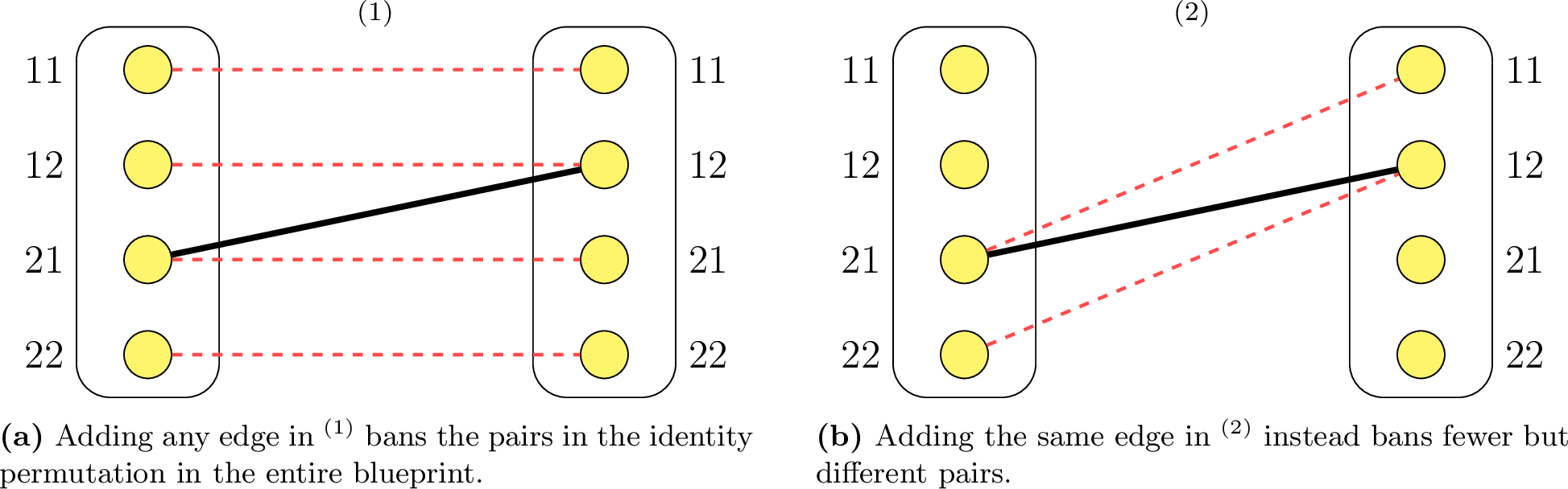
Finally, the following quantity determines how “good” a blueprint is for our purpose.
Definition 3. Define the value of a blueprint \(\mathbb{G}= (\mathbb{L},\mathbb{R},\mathbb{E})\) as: \[value(\mathbb{G}) := \frac{\left\vert{\mathbb{E}}\right\vert}{\left\vert{\mathbb{L}}\right\vert} = \frac{\left\vert{\mathbb{E}}\right\vert}{\left\vert{\mathbb{R}}\right\vert} = \frac{\left\vert{\mathbb{E}}\right\vert}{C^P}.\]
We refer the reader to [5] for several examples of blueprints and the intuition (and the formal proof) behind the connection between blueprints and semi-streaming matching. For us, we need the following theorem that captures the blueprint framework put forward in [5]3.
Theorem 2 (). Suppose there is a proper blueprint \(\mathbb{G}\) and define \(\alpha := \frac{2-2 \cdot value(\mathbb{G})}{2-value(\mathbb{G})}\). Then, for any fixed \(\delta > 0\), and any sufficiently large \(n\), as a function of \(\mathbb{G}\) and \(\delta\), the following holds. Any single-pass semi-streaming algorithm for maximum bipartite matching on \(n\)-vertex graphs cannot achieve an \((\alpha+\delta)\)-approximation with probability more than \(1-\delta\).
In [5], we constructed blueprints with values converging to \((5-\sqrt{10})/3\) which, plugged in 2, proves the impossibility of better than \((8-2\sqrt{10})/3 \sim 0.558\) approximation for the semi-streaming matching problem. The limit of the framework of [5] however is determined by the following quantity \[\begin{align} \sup\left\{ value(\mathbb{G}):\text{\mathbb{G} a proper blueprint} \right\}, \label{eq:sup} \end{align}\tag{1}\] which was not well understood in [5].
0.0.1.1.0.1 Our blueprint construction.
We determine the optimal value of 1 in this work, proving the following, which is the main technical result of our work.
Theorem 3. There is a sequence of proper blueprints \((\mathbb{G}_m)_{m \geqslant 1}\) with parameter \(P_m \to \infty\) and \[\lim_{m \to \infty} value(\mathbb{G}_m) = 2/3.\]
Plugging in the blueprints in 3 in 2 then immediately proves 1. Our proof of 3 is constructive and we give an explicit description of the blueprints in the family (even though this is not required to apply 2). We also note that as pointed out in [5], one does need \(P \to \infty\) for the value of the blueprint to be able to reach \(2/3\).
As an aside, we should note that, technically speaking, one also needs to prove an upper bound on 1 to fully determine the value of 1 (although this not needed for proving 1). However, a \(2/3\) upper bound follows immediately from 2 and the greedy algorithm for the semi-streaming matching problem. We give a different and direct proof of this upper bound in 0.0.5 as it provides further insight into the structure of blueprints.
0.0.1.2 Our Blueprint Construction at a High Level
We create the blueprints in 3 explicitly by using elementary properties of random walks on the integer line. The general idea of the construction is as follows (since our blueprint construction are entirely disjoint from [5] technique-wise, we will not review those constructions and refer the reader to [5] instead).
0.0.1.2.0.1 Vertices as random walks.
Let \(m \geqslant 1\) be an integer and \(\mathbb{G}= (\mathbb{L},\mathbb{R},\mathbb{E})\) be a blueprint with parameters \(P\) and \(C\) that depend on \(m\). Recall that vertices of \(\mathbb{G}\) are labeled by \([C]^P\). Suppose we pick \(x \in [C]^P\) uniformly at random: we assign to \(x\) a random walk \(W(x)\) on \(\left\{ 0,\ldots,2m \right\}\) that starts from a state in \([2m-1]\) chosen according to a distribution \(\mu\) that will be chosen later, and in each step moves in either direction uniformly until it reaches \(0\) or \(2m\). Moreover, define the reflection walk \(\overline{W}(x)\) that starts at the same state as \(W(x)\) but then in every step, takes the opposite direction as \(W(x)\). The assignment of \(W(x)\) to \(x\) is simply done by using the first index of \([P]\) to simulate sampling from \(\mu\) (by partitioning \([C]\) into lengths \(\propto \mu(i)\)-values) and remaining indices to simulate the random walk (by partitioning \([C]\) into two equal halves); see 2 for a quick illustration (we have skipped one other coordinate in \([P]\) called “delay” and will explain it later).
0.0.1.2.0.2 Edges between \(0\)-reaching random walks.
Let \(\mathbb{L}^{\star}\) (resp. \(\mathbb{R}^{\star}\)) be vertices \(\mathbb{L}(x)\) (resp. \(\mathbb{R}(x)\)) whose random walk \(W(x)\) (resp. \(\overline{W}(x)\)) reaches \(0\) (we emphasize that both are defined to reach \(0\)). Moreover, for any \(j \in [2m-1]\) and time \(t \in [P-1]\), let \(\mathbb{L}^{\star}_{j,t}\) denote the following subset of \(\mathbb{L}^{\star}\):
- All \(\mathbb{L}(x) \in \mathbb{L}\) such that \(W(x)\) reaches \(0\), \(W(x)\) has \(j\) as the maximum state it ever visits, and, it has visited \(j\) for the first time at the \(t\)-th step of the walk.
We define \(\mathbb{R}^{\star}_{j,t}\) analogously using the reflection walk \(\overline{W}\). In the blueprint, we add an edge between \(\mathbb{L}^{\star}_{j,t}\) and \(\mathbb{R}^{\star}_{2m-j,t}\) in \(\mathbb{E}^{(t+1)}\) with size equal to the smaller of the two.
0.0.1.2.0.3 Properness of the blueprint.
We need to ensure the inserted edges form a matching and that the ban constraints are satisfied. The former is easy to verify as \(\mathbb{L}^{\star}_{j,t},\mathbb{R}^{\star}_{j,t})\) sets are disjoint for different \(j,t\) and each is incident on a matching. We now prove the ban constraint.
Consider any edge between \(\mathbb{L}(x) \in \mathbb{L}^{\star}_{j,t}\) and \(\mathbb{R}(y) \in \mathbb{R}^{\star}_{2m-j,t}\) in some \(\mathbb{E}^{(t+1)}\) for \(j \in [2m-1]\) and \(t \in [P-1]\) (all edges of are of this form). The ban constraint requires that for any \(z \in [C]^{P-t}\), at most one of \(\mathbb{L}(x_{\leqslant t} \circ z)\) or \(\mathbb{R}(x_{\leqslant t} \circ z)\) is matched. Fixing of \(x_{\leqslant t}\) and \(y_{\leqslant t}\) “bring” any walk of \(W(x_{\leqslant t} \circ z)\) and \(\overline{W}(x_{\leqslant t} \circ z)\) to the states \(j\) and \(2m-j\) at their \(t\)-th step (by the definitions of \(\mathbb{L}^{\star}_{j,t},\mathbb{R}^{\star}_{2m-j,t}\)). Now, suppose \(\mathbb{L}(x_{\leqslant t} \circ z)\) is matched. Then, it means that the remainder of the walk, which with a slight abuse of notation we denote by \(W(z)\), will move from the state \(j\), uses \(z\), and reaches \(0\) (so \(\mathbb{L}(x_{\leqslant t} \circ z)\) becomes matched). But then, the reflection walk \(\overline{W}(z)\) will move in the “opposite” direction: it moves from \(2m-j\), uses \(z\), and thus reaches \(2m\) instead; this means that \(\mathbb{R}(y_{\leqslant t} \circ z)\) will not be matched, as desired. This is the entire proof of the ban constraint.
0.0.1.2.0.4 Value calculation.
The final step is to consider the value of this blueprint. In our construction, we are going to ensure that sizes of each of \(\mathbb{L}^{\star}_{j,t}\) and \(\mathbb{R}^{\star}_{2m-j,t}\) that are matched together is almost equal to each other. This will ensure that size of the matching of the blueprint is (essentially) \(\mathbb{L}^{\star}\), which implies that \[\begin{align} value(\mathbb{G}) = \frac{\left\vert{\mathbb{L}^{\star}}\right\vert}{C^P} = \mathop{\mathrm{\textrm{Pr}}}_{x \in_R [C]^P}\left(\text{walk W(x) reaches 0}\right). \label{eq:over-value} \end{align}\tag{2}\] As stated earlier, the constraint we have is that \(\mathbb{L}^{\star}_{j,t}\) and \(\mathbb{R}^{\star}_{2m-j,t}\) sets should have roughly the same size. For now let us relax this constraint to instead ask \(\mathbb{L}^{\star}_{j} := \cup_t~ \mathbb{L}^{\star}_{j,t}\) and \(\mathbb{R}^{\star}_{2m-j} := \cup_t~ \mathbb{R}^{\star}_{j,t}\) have the same size. This translates to having, \[\begin{align} &\forall j \in [2m-1] \mathop{\mathrm{\textrm{Pr}}}_{x \in_R [C]^P}\left(\text{walk W(x) reaches 0 and maximum state it visits is j}\right) \notag \\ &= \mathop{\mathrm{\textrm{Pr}}}_{x \in_R [C]^P}\left(\text{walk \overline{W}(x) reaches 0 and maximum state it visits is 2m-j}\right). \label{eq:over-constraint} \end{align}\tag{3}\] The underlying distributions of both \(W(x)\) and \(\overline{W}(x)\) here are just standard random walks starting from a random state chosen according to some distribution \(\mu\). Thus, at this point, the goal is to maximize 2 subject to the constraints in 3 , by choosing the initial distribution \(\mu\) carefully.
The type of random walk we have here is often called “gambler’s ruin” and are well studied as one of the simplest examples of Markov Chains; see, e.g. [29]. For instance, it is known that starting from a uniform distribution \(\mu\), maximum visited state will also be distributed uniformly and thus certainly satisfies 3 . But in this case, the walk has an equal chance of reaching \(0\) and \(2m\), making \(value(\mathbb{G})=1/2\) only. However, by “shifting” the distribution of \(\mu\) towards \(0\), while still enforcing 3 , one can improve the objective function. We are not aware of prior work that study this particular formulation but solving this optimization problem has a standard method: one can cast the problem as a linear program in \(\mu(i)\)-values and obtain a closed form formula for the variables. Doing this in our case leads to the objective value of \(2m/(3m+1)\) (see 7), giving us the desired value for the blueprint.
There is however one catch with the argument above: we moved from enforcing (near) equality in sizes of \(\mathbb{L}^{\star}_{j,t}\) and \(\mathbb{R}^{\star}_{2m-j,t}\) to only \(\mathbb{L}^{\star}_j\) and \(\mathbb{R}^{\star}_{2m-j}\); but, symmeterizing the distribution of maxima (through the choice of \([m]\)) does not mean the time to reaching them will also be symmetric. This however can be handled rather easily by introducing random delays in the random walks: we dedicate one more coordinate in \([P]\) for this task, and start the random walks at different time stages to ensure that distribution of “time to hit maximum” becomes (almost) uniform over the time steps which fixes the above problem.
0.0.1.3 Further Corollaries of Our Result
We mention two further corollaries of our results. The first one is for the matching problem but in another model, the online matching with preemption, whereas the second one is for another problem, the minimum vertex cover, but back in the semi-streaming model.
0.0.1.3.0.1 Online matching with preemption.
In this problem, the edges of the graph are arriving sequentially and the algorithm must maintain a matching by accepting or rejecting arriving edges and can preempt previously accepted ones by discarding them. This model is a generalization of the original online matching (with one-sided vertex arrival) in [30].
The competitive ratio of an algorithm in this model is the ratio of the matching size provided by the algorithm compared to the maximum matching of the graph. The greedy algorithm achieves a half competitive ratio in this model with no need for preemption. When preemptions are not allowed, [31] proved that half approximation is optimal. No better algorithm are known even with allowing preemption and a series of results over the years have ruled out competitive ratios of \((1-1/e) \sim 0.632\) [30], \((1+\ln{(2)})^{-1} \sim 0.590\) [32], \((2-\sqrt{2}) \sim 0.585\) [33], and very recently \(0.5661\) [34]4. We prove that the greedy algorithm is also optimal for this problem.
Corollary 1. There is no algorithm for the online matching problem with preemption with an expected competitive ratio strictly better than half by any constant.
As already observed in [5], the blueprint framework also implies lower bounds for the online matching problem with preemption (given this connection, technically, the best known bound on the competitive ratios prior to our work is the \(0.558\) bound of [5], which was obtained independently and concurrently to [34]). Thus, 1 directly follows from our 3 and the blueprint framework of [5].
0.0.1.3.0.2 Semi-streaming (bipartite) vertex cover.
Going back to the semi-streaming model, a closely related problem to maximum bipartite matching is its dual, the minimum bipartite vertex cover problem. The greedy algorithm is also a \(2\)-approximation algorithm for this problem and no better algorithms are known. It has been asked in prior work, e.g., [16], [35] whether this algorithm can be improved. We resolve this question in this work.
Corollary 2. There is no single-pass semi-streaming algorithm for the minimum bipartite vertex cover problem that can achieve any constant approximation ratio strictly better than two with constant probability.
We note that prior to our work, no \(2\)-approximation lower bounds were known for this problem even in general graphs (the UGC hardness of \(2\)-approximation vertex cover [36] does not imply a semi-streaming lower bound, as runtime of algorithms is not bounded in this model).
The proof of this result is again by observing that the blueprint framework of [5] also implies lower bounds for the vertex cover problem given the duality of the problems (plus a standard modification for going from matching lower bounds to vertex cover ones as done previously in the literature, e.g., in [16], [37]).
0.0.2 Preliminaries↩︎
0.0.2.0.0.1 Notation.
For integers \(1 \leqslant a \leqslant b\), we define \([a:b] := \left\{ a,a+1,\ldots,b \right\}\) and \([b] := \left\{ 1,\ldots,b \right\}\). For a tuple \(x=(x_1,\ldots,x_t)\) and \(i \in [2:t]\), we denote \(x_{<i} := (x_1,\ldots,x_{i-1})\).
For a random variable \(X\), we sometimes write the subscript \(X\) in \(\mathop{\mathrm{\textrm{Pr}}}_X(f(X))\) (for some \(f\)), to explicitly specify the randomness is coming from \(X\). For a random variable \(X\) and a set \(S\), we write \(X \in_R S\) to mean \(X\) is sampled uniformly at random from \(S\).
0.0.2.0.0.2 Gambler’s ruin.
We use a standard type of random walks on integer line \(\left\{ 0,1,\ldots,2m \right\}\) for some integer \(m \geqslant 1\), often called the gambler’s ruin; see, e.g. [29].
The walk \(W=w_1,w_2,\cdots\) starts at some integer \(w_1 \in [2m-1]\) and in each time \(t \geqslant 1\), it updates \(w_{t+1} = w_{t}+1\) with probability half and \(w_{t+1} = w_{t}-1\) otherwise. The walk terminates at the first time \(t\) when \(w_t = 0\) or \(w_t = 2m\) and remains in this state. Throughout, by a random walk, we always mean the above type of walk unless explicitly stated otherwise.
Fact 4 (c.f. [29]). For a random walk \(W\) over and an integer \(k\) in \(\left\{ 0,\ldots,2m \right\}\), \[\mathop{\mathrm{\textrm{Pr}}}_{W}\left(\text{W reaches 0 before 2m} \mid \text{W starts at k}\right) = \frac{2m-k}{2m}.\] Moreover, the expected length of the walk before terminating is at most \(m^2\).
For a (finite) random walk \(W = w_1,\cdots,w_T\), where \(w_1\) is the starting state and \(w_T \in \left\{ 0,2m \right\}\) is a terminating state, we define: \[\begin{align} \textrm{\textsf{w}}_{\textrm{max}}&= \textrm{\textsf{w}}_{\textrm{max}}(W) := \max_{t \in [T]} \left\{ w_t \right\} \quad \text{and}\quad \textrm{\textsf{t}}_{\textrm{max}}= \textrm{\textsf{t}}_{\textrm{max}}(W) := \min \left\{ t \in [T] : w_t=\textrm{\textsf{w}}_{\textrm{max}}(W) \right\}, \end{align}\] as the largest state seen on the walk and the first time the walk sees its eventual largest state.
A corollary of 4 is the following.
Claim 5. For a random walk \(W\) over \(\left\{ 0,\ldots,2m \right\}\) and any \(1 \leqslant i \leqslant j < 2m\), \[\mathop{\mathrm{\textrm{Pr}}}_W\left(\text{W ends in 0} \wedge \textrm{\textsf{w}}_{\textrm{max}}(W) = j \mid \text{W starts at i}\right) = \frac{i}{j \cdot (j+1)}.\]
Proof. For this to happen, we need \(W\) to reach \(j\) before \(0\), and once on \(j\), to reach \(0\) before \(j+1\). Given the random walk is memoryless, these two events are independent and thus we have \[\begin{align} &\mathop{\mathrm{\textrm{Pr}}}_W\left(\text{W ends in 0} \wedge \textrm{\textsf{w}}_{\textrm{max}}(W) = j \mid \text{W starts at i}\right) = \\ & \mathop{\mathrm{\textrm{Pr}}}_W\left(\text{W reaches j before 0} \mid \text{W starts at i}\right) \cdot \mathop{\mathrm{\textrm{Pr}}}_W\left(\text{W reaches 0 before j+1} \mid \text{W starts at j}\right). \end{align}\] The first term is about a random walk on \(\left\{ 0,\ldots,j \right\}\) starting from \(i\) and thus by 4 has probability \(i/j\). The second term is about a random walk on \(\left\{ 0,\ldots,j+1 \right\}\) starting from \(j\) and thus by 4 has probability \(1/(j+1)\). Multiplying these two concludes the proof. ◻
We also have the following standard claim on the length of random walks.
Claim 6. The probability that a random walk \(W\) starting from any state does not terminate within \(2m^3\) steps is at most \(2^{-m}\).
Proof. The expected time for a walk \(W\) to terminate, starting from any state, is at most \(m^2\) by 4. Thus, by Markov bound, the probability that the walk has not terminated after \(2m^2\) steps is at most half. Repeating the argument from current state, the probability that \(m\) repetitions, each of length \(2m^2\), does not terminate the walk is at most \(2^{-m}\). ◻
0.0.3 Random Walk on a Line with Symmetric Maxima↩︎
Fix any integer \(m \geqslant 1\). We will be using the gambler’s ruin random walk on \(\left\{ 0,\ldots,2m \right\}\) described in 0.0.2 for our proofs. For our purpose, we also need to specify a distribution over initial states with the following two properties: (1) the distribution of \(\textrm{\textsf{w}}_{\textrm{max}}(W)\) is symmetric (on the interior states) assuming the start state is sampled from this distribution, and, (2) the probability of terminating in state \(0\) is maximized. The following lemma finds such a distribution for us (we do not explicitly prove that it maximizes the term in \((2)\) and only calculate its value, which is sufficient for us; however, one can prove it is maximized).
Lemma 7. Consider the assignment \(\mu: \left\{ 1,\ldots,2m-1 \right\} \rightarrow [0,1]\) such that for \(i \in [m]\), \[\mu(i) := \gamma_{m} \cdot \frac{2 \cdot (2m+1)}{(2m-i)\cdot(2m-i+1)\cdot(2m-i+2)} \quad \text{for} \quad \gamma_m := \frac{2m \cdot (m+1)}{3m+1},\] and for \(i \in [m+1:2m-1]\), \(\mu(i)=0\).
Firstly, \(\mu\) is a distribution. Secondly, if we sample a random walk \(W\) starting from a state distributed according to \(\mu\)—denoting the combined distribution by \(\mathcal{D}_m\)—, then, for all \(j \in [2m-1]\), \[\mathop{\mathrm{\textrm{Pr}}}_{W \sim \mathcal{D}_m}\left(\text{W\!~ends in 0} ~\wedge~ \textrm{\textsf{w}}_{\textrm{max}}(W) = j\right) = \mathop{\mathrm{\textrm{Pr}}}_{W \sim \mathcal{D}_m}\left(\text{W\!~ends in 0} ~\wedge~ \textrm{\textsf{w}}_{\textrm{max}}(W) = 2m-j\right).\] Finally, \[\mathop{\mathrm{\textrm{Pr}}}_{W \sim \mathcal{D}_m}\left(\text{W\!~ends in 0}\right) = \frac{2m}{3m+1}.\]
We postpone the proof of this lemma to the end of this section to complete our definitions first. The proof can be skipped by the reader as it is not needed for understanding the rest of the paper.
0.0.3.0.0.1 Delayed and length-restricted random walks.
7 “symmetrizes” the distribution of maxima for a random walk \(W\). We also need to ensure the distribution of the time of reaching the maxima is (essentially) the same across different choices for \(\textrm{\textsf{w}}_{\textrm{max}}(W)\). Adding a “delay” to the walk fixes this issue as well.
A delayed random walk with delay \(d \geqslant 1\) (also called \(d\)-delayed random walk) is defined similar to our original random walk, except that for its first \(d\) time steps, the walk stays in the same state and starts moving as before from time step \(d+1\). Specifically, a \(d\)-delayed random walk \(W=w_1,w_2,\cdots,\) is such that \[w_1 = \cdots = w_d \quad \text{and} \quad \text{for t \geqslant d,}~ w_{t+1}~\text{is chosen uniformly from}~\left\{ w_t + 1 , w_t-1 \right\},\] and the walk as before terminates when hitting the state \(0\) or \(2m\). We refer to the “non-delayed” part of the walk \(W\) as the inner random walk \(W_{in}\), namely, \(W_{in} = w_d, w_{d+1},\cdots\).
For a \(d\)-delayed random walk \(W\), we define \[\begin{align} \textrm{\textsf{t}}_{\textrm{max}}(W) = (d-1)+\textrm{\textsf{t}}_{\textrm{max}}(W_{in}), \label{eq:timemaxW} \end{align}\tag{4}\] namely, the time the inner walk reached the eventual maximum (this distinction between inner and the entire walk is only relevant when the starting state is the eventual maximum; in this case, we consider \(\textrm{\textsf{t}}_{\textrm{max}}(W)=d\), namely, the delay of the walk instead of time \(0\)); \(\textrm{\textsf{w}}_{\textrm{max}}(W)\) is defined as before which is equal to \(\textrm{\textsf{w}}_{\textrm{max}}(W_{in})\) regardless.
Finally, we also need the length of the walks to be finite, which can be guaranteed (essentially) by 6. We say that a delayed random walk is \(\ell\)-length restricted iff it terminates within \(\ell\) steps after spending its delayed time, i.e., reaches states \(0\) or \(2m\) within \(d+\ell\) steps assuming its delay was \(d\) (or alternatively, the length of its inner walk \(W_{in}\) is at most \(\ell\)). By 6, for large enough \(\ell\), a (delayed) random walk will be \(\ell\)-length restricted with high probability (in \(m\)).
0.0.3.1 Proof of 7
We remark that the “right” way to prove a statement of the type 7 is to solve the program that maximizes \(\mathop{\mathrm{\textrm{Pr}}}(\text{W ends in 0})\) subject to the symmetric constraints, under variables \(\left\{ \mu(i) \right\}_{i=1}^{2m-1}\) which are non-negative and sum to one. This becomes a linear programming problem which can then be solved explicitly (by considering its dual), to determine the values of \(\mu(i)\)’s. Nevertheless, since we have already solved this program and obtained \(\mu(i)\)’s, in the following proof we only verify the correctness of these variables.
We prove each part of 7 in the following.
0.0.3.1.0.1 \(\mu\) forms a distribution.
Clearly, all \(\mu(i) \geqslant 0\) so we only need to prove \(\sum_i \mu(i)=1\). For this, \[\begin{align} \sum_i \mu(i) &= \gamma_m \cdot \sum_{i=1}^{m} \frac{2 \cdot (2m+1)}{(2m-i)\cdot(2m-i+1)\cdot(2m-i+2)} \\ &= \gamma_m \cdot \sum_{r=m}^{2m-1} \frac{2 \cdot (2m+1)}{r \cdot (r+1)\cdot(r+2)}\\ &= \gamma_m \cdot \sum_{r=m}^{2m-1} (2m+1) \cdot \left(\frac{1}{r \cdot (r+1)} - \frac{1}{(r+1)\cdot(r+2)}\right)\\ &= \gamma_m \cdot (2m+1) \cdot \left(\frac{1}{m \cdot (m+1)} - \frac{1}{(2m)\cdot(2m+1)}\right)\\ &= \gamma_m \cdot \frac{3m+1}{2m \cdot (m+1)} = 1, \end{align}\] by the definition of \(\gamma_m\). Thus, \(\mu\) is a distribution.
0.0.3.1.0.2 Symmetric property.
To simplify the notation, in the following, we use ‘\(w_T=0\)’ to denote the event that the walk ends in \(0\) (instead of \(2m\)) and use ‘\(w_1=i\)’ for any integer \(i\) to mean the walk starts from the state \(i\). For any \(j \in [2m-1]\), \[\begin{align} \mathop{\mathrm{\textrm{Pr}}}_{W \sim \mathcal{D}_m}\left(w_T=0 ~\wedge~ \textrm{\textsf{w}}_{\textrm{max}}(W) = j\right) &= \sum_{i=1}^{m} \mu(i) \cdot \mathop{\mathrm{\textrm{Pr}}}\left(w_T=0 ~\wedge~ \textrm{\textsf{w}}_{\textrm{max}}(W) = j \mid w_1=i\right)\\ &= \sum_{i=1}^{\min(m,j)} \mu(i) \cdot \mathop{\mathrm{\textrm{Pr}}}\left(w_T=0 ~\wedge~ \textrm{\textsf{w}}_{\textrm{max}}(W) = j \mid w_1=i\right) }_{\textrm{max}}(W)=j never happens} \\ &= \sum_{i=1}^{\min(m,j)} \mu(i) \cdot \frac{i}{j \cdot (j+1)}, \label{eq:get-back-to} \end{align}\tag{5}\] by 5 since \(1 \leqslant i \leqslant j \leqslant 2m\). We have the following claim on partials sums above.
Claim 8. For any \(j \in [m]\), \[P_j := \sum_{i=1}^{j} \mu(i) \cdot i = \gamma_m \cdot \frac{j \cdot (j+1)}{(2m-j) \cdot (2m-j+1)}.\]
Proof. The proof is by induction. For \(j=1\), \[P_1 = \mu(1) = \gamma_{m} \cdot \frac{2 \cdot (2m+1)}{(2m-1)\cdot(2m)\cdot(2m+1)} = \gamma_{m} \cdot \frac{1 \cdot (1+1)}{(2m-1)\cdot(2m)},\] matching the RHS of the claim. For \(1 < j \leqslant m\), for the induction step, by the value of \(\mu(j)\), \[\begin{align} P_j = P_{j-1} + j \cdot \mu(j) &= \gamma_m \cdot \frac{(j-1) \cdot j}{(2m-j+1) \cdot (2m-j+2)} + j \cdot \gamma_{m} \cdot \frac{2 \cdot (2m+1)}{(2m-j)\cdot(2m-j+1)\cdot(2m-j+2)} \\ &= \gamma_m \cdot \frac{{j \cdot (j-1) \cdot (2m-j)+2j \cdot (2m+1)}}{(2m-j)\cdot(2m-j+1)\cdot(2m-j+2)} \\ &= \gamma_m \cdot \frac{j \cdot (j+1)}{(2m-j) \cdot (2m-j+1)}, \end{align}\] where the last equation can be verified using a direct calculation by verifying that \[(2m-j+2) \cdot (j+1) = (j-1) \cdot (2m-j)+2\cdot (2m+1).\] This concludes the proof. ◻
Plugging in 8 in 5 , we have that for any \(j \in [m]\), \[\mathop{\mathrm{\textrm{Pr}}}_{W \sim \mathcal{D}_m}\left(w_T=0 ~\wedge~ \textrm{\textsf{w}}_{\textrm{max}}(W) = j\right) = \frac{P_j}{j \cdot (j+1)} = \gamma_m \cdot \frac{1}{(2m-j) \cdot (2m-j+1)}.\] On the other hand, for \(j \in [m]\), we have \(2m-j \geqslant m\) and by the max-term in 5 , \[\mathop{\mathrm{\textrm{Pr}}}_{W \sim \mathcal{D}_m}\left(w_T=0 ~\wedge~ \textrm{\textsf{w}}_{\textrm{max}}(W) = 2m-j\right) = \frac{P_m}{(2m-j) \cdot (2m-j+1)} = \gamma_m \cdot \frac{1}{(2m-j) \cdot (2m-j+1)},\] since by 8, \(P_m =\gamma_m\). This proves the equality in the symmetric property.
0.0.3.1.0.3 Probability of \(W\) ending in \(0\).
We calculate this directly as \[\begin{align} \mathop{\mathrm{\textrm{Pr}}}_{W \sim \mathcal{D}_m}\left(w_T=0\right) &= \sum_{i=1}^{m} \mu(i) \cdot \mathop{\mathrm{\textrm{Pr}}}_{W}\left(w_T=0 \mid w_1=i\right)\\ &= \sum_{i=1}^{m} \mu(i) \cdot \mathop{\mathrm{\textrm{Pr}}}_{W}\left(\text{W reaches 0 before 2m} \mid w_1=i\right)\\ &= \sum_{i=1}^{m} \mu(i) \cdot \frac{2m-i}{2m} } \\ &= 1- \sum_{i=1}^{m} \frac{i \cdot \mu(i)}{2m}\\ &= 1- \frac{\gamma_m}{2m} } \\ &= \frac{2m}{3m+1}, \end{align}\] by the value of \(\gamma_m\). This concludes the proof of 7. height0.75em width0.5em depth0.25em
0.0.4 The Blueprint Construction↩︎
We provide our blueprint construction in this section, proving the following theorem.
Theorem 1 (Restatement of 3). For any sufficiently large integer \(m\), there exists a proper blueprint \(\mathbb{G}_m\) with parameters \(P=\rm poly(m)\) and \(C=m^{O(m)}\) such that \[value(\mathbb{G}_m) = \frac{2}{3} - \Theta\!\left(\frac{1}{m}\right).\]
We start by presenting the setup needed for this construction, followed by the construction itself and its properness proof, and finally calculate its value to conclude the proof of 3.
0.0.4.1 Setup
Let \(m\) be a large integer that is used to define all our other parameters for the blueprint. We define a blueprint \(\mathbb{G}:= \mathbb{G}(m)\) in this section. Define: \[\begin{align} L &:= m^4,of random walks} \\ D &:= 2m \cdot L,in random walks} \\ P &:= L+D+1\\ C &:= \text{sufficiently large as function of m to be fixed later} . \end{align}\] Recall that vertices of \(\mathbb{G}\) are \(\mathbb{L},\mathbb{R}\) and they are labeled by \([C]^{P}\). We partition indices of \(P\) as follows: \[\begin{gather} P := (\textrm{\texttt{start}}, \textrm{\texttt{delay}}, \textrm{\texttt{walk}}) \quad \text{where} \\ \textrm{\texttt{start}}=1, \quad \textrm{\texttt{delay}}=2, \quad \text{and,} \quad {\textrm{\texttt{walk}}} = [3: P]. \end{gather}\]
We use these indices to associate a delayed random walk to vertices of the blueprint as follows.
Definition 9. Sample \(x \in [C]^P\) uniformly at random and define a delayed random walk \(W = W(x) = w_1,w_2,\cdots,w_T\) for some \(T \leqslant D+L\) as follows5.
\(x_{\textrm{\texttt{start}}}\) determines the start state \(w_1\) of the random walk \(W\): we partition \([C]\) into intervals of proportional length \(\mu(1),\mu(2),\ldots,\mu(m)\) (as defined in 7), and pick \(w_1\) depending on which interval \(x_{\textrm{\texttt{start}}}\) lands in.
\(x_{\textrm{\texttt{delay}}}\) determines the delay of the delayed random walk \(W\): we partition \([C]\) into \(D\) equal-length intervals and the delay of the random walk \(d(x)=d\) if \(x_{\textrm{\texttt{delay}}}\) lands in \(d\)-th interval.
\(x_{\textrm{\texttt{walk}}}\) determines the inner walk: for any time \(t \geqslant d(x)\), \(x_{t+2}\) determines the transition from \(w_t\) to \(w_{t+1}\) in \(W\), where \(w_{t+1} = w_t -1\) if \(x_{t+2} \in [1:{C}/{2}]\) and \(w_{t+1}=w_t + 1\) otherwise. The walk terminates whenever it hits \(0\) or \(2m\) and the subsequent states remain the same.
We also define the reflection walk of \(x\), denoted by \(\overline{W}(x)\), exactly as \(W(x)\) except for Line [line:reflection]: we now increase the state if \(x_i \in [1:C/2]\) and decrease it otherwise (the exact opposite rule as in the definition of \(W\)).
See 2 for an illustration of this definition and further help with parsing it.
Before getting to the main part, a quick remark is in order.
Remark 10. We pick \(C\) such that
\(\mu(i) \cdot C\) is an integer for all \(i \in [2m-1]\) (so the distribution of the start point in Line [line:pstart] matches \(\mu\));
\(D | C\) (so the distribution of the delay in Line [line:pdelay] is uniform over \([D]\));
\(C\) is even (so the distribution of the inner walk in Line [line:reflection] is a standard random walk).
We can thus set \[C = 2D \cdot \prod_{i=1}^{m} \textrm{denominator of \mu(i)}\] and given the values of parameters \(\mu(i)\) in 7 and since \(D= \rm poly(m)\), we have \(C=m^{O(m)}\).
![Figure 2: An illustration of the random walk W(x) in 9 when m=3 and D=6. The figure shows how the indices of [P] are partitioned into (\textrm{\texttt{start}},\textrm{\texttt{delay}},\textrm{\texttt{walk}}). The intervals inside each box shows how [C] is partitioned into different intervals. The tiny arrows in each box shows the value of a single point x \in[C]^P on each relevant index. The walk W(x) thus first considers x_{\textrm{\texttt{start}}} and so chooses starting state 2. The delay d is set to 5 given x_{\textrm{\texttt{delay}}}. Finally, the walk waits until time d and then decide its next move based on the index d+2 and so on; in this particular example, the walk goes to 3 next, then 2, and then 1.](/article/2607.14656/_pdflatex/hsurzbjt.png "fig:")
We use walks \(W(x)\) for defining subsets of \(\mathbb{L}\) and reflection walks \(\overline{W}(x)\) for subsets in \(\mathbb{R}\). Specifically, for any integer \(j \in [2m]\) and time \(t \in [D+L]\), we define \[\begin{align} \mathbb{L}_{j,t} &:= \left\{ \mathbb{L}(x) : \text{W(x) is L-restricted, W(x) reaches 0, \textrm{\textsf{w}}_{\textrm{max}}(W(x))=j, and \textrm{\textsf{t}}_{\textrm{max}}(W(x)) = t} \right\}, \\ \mathbb{R}_{j,t} &:= \left\{ \mathbb{R}(x) : \text{\overline{W}(x) is L-restricted, \overline{W}(x) reaches 0, \textrm{\textsf{w}}_{\textrm{max}}(\overline{W}(x))=j, and \textrm{\textsf{t}}_{\textrm{max}}(\overline{W}(x)) = t} \right\}. \end{align}\] These sets will play the key role in the definition of edges of the blueprint (they are essentially the endpoints of the edges).
We have the following immediate relation between the sizes of these sets.
Claim 11. For all \(j \in [2m-1]\) and \(t \in [D+L]\), \(\left\vert{\mathbb{L}_{j,t}}\right\vert = \left\vert{\mathbb{R}_{j,t}}\right\vert\).
Proof. The only difference between \(\mathbb{L}_{j,t}\) and \(\mathbb{R}_{j,t}\) is in Line [line:reflection] of 9: we thus have \(\mathbb{L}(x) \in \mathbb{L}_{j,t}\) iff \(\mathbb{R}(\overline{x}) \in \mathbb{R}_{j,t}\), where \(\overline{x}\) is defined to be the same as \(x\) in \([P] \setminus \textrm{\texttt{walk}}\) and for \(i \in \textrm{\texttt{walk}}\), \(\overline{x}_i := C - x_i + 1\). Using the bijection between \(x\)’s and \(\overline{x}\)’s, we can conclude the proof. ◻
The more interesting property is the near-equality of the sizes of \(\mathbb{L}_{j,t}\) and \(\mathbb{R}_{2m-j,t}\) (whenever \(t \in [L:D]\)); this is where we use most of the properties we incorporated in our random walks.
Lemma 12. For all \(j \in [2m-1]\) and \(t \in [L:D]\), \[\left\vert{\mathbb{R}_{2m-j,t}}\right\vert - 2^{-m} \cdot \frac{C^P}{D} \leqslant\left\vert{\mathbb{L}_{j,t}}\right\vert \leqslant\left\vert{\mathbb{R}_{2m-j,t}}\right\vert + 2^{-m} \cdot \frac{C^P}{D}.\]
Proof. Define \(W_{in}(x)\) as the inner walk of \(W(x)\), which is the walk that starts at time \(d(x)\) (the delay) and continues the same as \(W\); we define \(\overline{W}_{in}(x)\) similarly. In the following, when clear from the context, we drop \((x)\) and write \(W\) to denote \(W(x)\) (similarly for \(W_{in},\overline{W}\), etc.).
We first have \[\begin{align} \frac{\left\vert{\mathbb{L}_{j,t}}\right\vert}{C^P} &= \mathop{\mathrm{\textrm{Pr}}}_{x}\Big(\text{W L-restricted, W reaches 0, \textrm{\textsf{w}}_{\textrm{max}}(W)=j, \textrm{\textsf{t}}_{\textrm{max}}(W) = t}\Big) }\\ &= \mathop{\mathrm{\textrm{Pr}}}_{x}\Big(\text{W_{in} L-restricted, W_{in} reaches 0, \textrm{\textsf{w}}_{\textrm{max}}(W_{in})=j, \textrm{\textsf{t}}_{\textrm{max}}(W) = t}\Big)and W} \\ &= \mathop{\mathrm{\textrm{Pr}}}_{x}\Big(\text{W_{in} L-restricted, W_{in} reaches 0, \textrm{\textsf{w}}_{\textrm{max}}(W_{in})=j, \textrm{\textsf{t}}_{\textrm{max}}(W_{in}) = t-(d(x)-1)}\Big) }_{\textrm{max}}(W) in~\Cref{eq:timemaxW}} \\ &= \frac{1}{D} \cdot \mathop{\mathrm{\textrm{Pr}}}_{x}\Big(\text{W_{in} L-restricted, W_{in} reaches 0, \textrm{\textsf{w}}_{\textrm{max}}(W_{in})=j}\Big) \end{align}\] as \(d(x)\) is independent of \(W_{in}\) and is uniform over \([D]\), and so the event \(d(x) = t-\textrm{\textsf{t}}_{\textrm{max}}(W_{in})+1\) (conditioned on \(W_{in}\)) happens with probability \(1/D\) as the RHS is in \([D]\) as well; this is because \(\textrm{\textsf{t}}_{\textrm{max}}(W_{in}) \leqslant L\) (by \(L\)-restrictedness) and \(t \in [L:D]\).
We can do the same exact analysis for \(\mathbb{R}_{2m-j,t}\) and \(\overline{W}\) as well to have \[\frac{\left\vert{\mathbb{R}_{2m-j,t}}\right\vert}{C^P} = \frac{1}{D} \cdot \mathop{\mathrm{\textrm{Pr}}}_{x}\Big(\text{\overline{W}_{in} L-restricted, \overline{W}_{in} reaches 0, \textrm{\textsf{w}}_{\textrm{max}}(\overline{W}_{in})=2m-j}\Big).\] Consider the expression in the RHS of either of these two terms. The distribution of \(W_{in}\) or \(\overline{W}_{in}\) is exactly the same as the distribution of a random walk \(\widetilde{W} \sim \mathcal{D}_m\) defined in 7. Hence, \[\begin{align} \frac{\left\vert{\mathbb{L}_{j,t}}\right\vert}{C^P} &= \frac{1}{D} \cdot \mathop{\mathrm{\textrm{Pr}}}_{\widetilde{W}}\Big(\text{\widetilde{W} L-restricted, \widetilde{W} reaches 0, \textrm{\textsf{w}}_{\textrm{max}}(\widetilde{W})=j}\Big) \\ &\geqslant\frac{1}{D} \cdot \left(\mathop{\mathrm{\textrm{Pr}}}_{\widetilde{W}}\Big(\text{\widetilde{W} reaches 0, \textrm{\textsf{w}}_{\textrm{max}}(\widetilde{W})=j}\Big) - \mathop{\mathrm{\textrm{Pr}}}_{\widetilde{W}}\Big(\text{\widetilde{W} not L-restricted}\Big)\right) }}(A \wedge B) \geqslant\mathop{\mathrm{\textrm{Pr}}}(B) - \mathop{\mathrm{\textrm{Pr}}}(\overline{A})} \\ &\geqslant\frac{1}{D} \cdot \left(\mathop{\mathrm{\textrm{Pr}}}_{\widetilde{W}}\Big(\text{\widetilde{W} reaches 0, \textrm{\textsf{w}}_{\textrm{max}}(\widetilde{W})=j}\Big) - 2^{-m}\right) } \\ &= \frac{1}{D} \cdot \left(\mathop{\mathrm{\textrm{Pr}}}_{\widetilde{W}}\Big(\text{\widetilde{W} reaches 0, \textrm{\textsf{w}}_{\textrm{max}}(\widetilde{W})=2m-j}\Big) - 2^{-m}\right) } \\ &\geqslant\frac{1}{D} \cdot \left(\mathop{\mathrm{\textrm{Pr}}}_{\widetilde{W}}\Big(\text{\widetilde{W} L-restricted, \widetilde{W} reaches 0, \textrm{\textsf{w}}_{\textrm{max}}(\widetilde{W})=2m-j}\Big) - 2^{-m}\right) }}(A) \geqslant\mathop{\mathrm{\textrm{Pr}}}(A \wedge B)} \\ &= \frac{\left\vert{\mathbb{R}_{2m-j,t}}\right\vert}{C^P} - \frac{2^{-m}}{D}. \end{align}\] Applying the same argument starting from \(\mathbb{R}_{2m-j,t}\) then implies that \[\left\vert{\mathbb{R}_{2m-j,t}}\right\vert - 2^{-m} \cdot \frac{C^P}{D} \leqslant\left\vert{\mathbb{L}_{j,t}}\right\vert \leqslant\left\vert{\mathbb{R}_{2m-j,t}}\right\vert + 2^{-m} \cdot \frac{C^P}{D} \nobreak \ifvmode \relax \else \ifdim\lastskip<1.5em \hskip-\lastskip \hskip 1.5em plus0em minus0.5em \fi \nobreak \vrule height0.75em width0.5em depth0.25em\fi\] ◻
0.0.4.2 The Construction
We are now ready to define the edges of the blueprint \(\mathbb{G}=(\mathbb{L},\mathbb{R},\mathbb{E})\) and prove its properness. As stated earlier, both vertex-sets \(\mathbb{L}\) and \(\mathbb{R}\) are labeled by \([C]^P\). The edges in \(\mathbb{E}\) are defined as follows:
- For any \(j \in [2m-1]\) and \(t \in [L:D]\), we add a matching \(\mathbb{M}_{j,t}\) of size \(s_{j,t} := \min\left(\left\vert{\mathbb{L}_{j,t}}\right\vert,\left\vert{\mathbb{R}_{2m-j,t}}\right\vert\right)\) between two arbitrarily-chosen \(s_{j,t}\)-subsets of \(\mathbb{L}_{j,t}\) and \(\mathbb{R}_{2m-j,t}\). Moreover, the matching \(\mathbb{M}_{j,t}\) is added as part of \(\mathbb{E}^{(p)}\) for \(p=t+2\).
We need to check that the blueprint \(\mathbb{G}\) is proper, which is handled by the following two claims.
Claim 13 (“Matching constraint”). The edge-set \(\mathbb{E}\) is a matching.
Proof. By definition, the sets \(\mathbb{L}_{j,t}\) are disjoint for different values of \(j\) (the maximum of a random walk is a unique state) as well as \(t\) (the first time reaching the eventual maximum is unique). Same is true for \(\mathbb{R}_{2m-j,t}\) as well, thus \(\mathbb{E}= \cup_{p \in [P]} \mathbb{E}^{(p)}\) itself is a matching also. ◻
![Figure 3: An illustration of the proof of the ban constraint (14) for \mathbb{G} with m=6, j=2, and z \approx (\uparrow,\uparrow,\downarrow,\downarrow,\downarrow,\downarrow), which by that we mean the \uparrow indices are in [(C/2)+1:C]and \downarrow ones are in [1:C/2]. Suppose the choices of x_{<p} and y_{<p} already “bring” the walks W(x_{<p} \circ z) and \overline{W}(y_{<p} \circ z) tostates 2 and 10, respectively. From there, W(x_{<p} \circ z), increases the state by two and then decreases it by four, whereas by reflection, \overline{W}(y_{<p} \circ z) does the exact opposite; thus,W(x_{<p} \circ z) reaches state 0 iff \overline{W}(y_{<p} \circ z) reaches 12 (=2m). As such, at most one pair of these vertices can be matched in \mathbb{G} (only vertices whose walk reaches 0 are matched regardless of being in \mathbb{L} or \mathbb{R}).](/article/2607.14656/_pdflatex/htbefjxm.png "fig:")
Claim 14 (“Ban constraint”). The edge-set \(\mathbb{E}\) respects the ban constraint.
Proof. Consider an edge \(\mathbb{e}\in \mathbb{E}^{(p)}\) for \(p=t+2\) for some arbitrary \(t \in [L:D]\) and suppose \(\mathbb{e}\) is between some \(\mathbb{L}(x) \in \mathbb{L}_{j,t}\) and \(\mathbb{R}(y) \in \mathbb{R}_{2m-j,t}\) for \(x,y \in [C]^P\). Recall all edges of \(\mathbb{G}\) are of this form.
By 2, the ban constraint requires that for all \(z \in [C]^{P-p+1}\), at most one of \(\mathbb{L}(x_{<p} \circ z)\) and \(\mathbb{R}(y_{<p} \circ z)\) is matched in \(\mathbb{E}\). We show that this is the case for every fixed \(z \in [C]^{P-p+1}\). 3 can be helpful with providing an illustration of this step of the proof.
Consider the walk \(W(x_{<p} \circ z)\). Fixing \(x_{<p}\) fixes the starting state of the walk (by fixing \(x_{\textrm{\texttt{start}}}\)), the delay of the walk (by fixing \(x_{\textrm{\texttt{delay}}}\)) and the states until time \(t\) of the walk. By the definition of \(\mathbb{L}(x) \in \mathbb{L}_{j,t}\), we know that at the time \(t\), the walk \(W(x_{<p} \circ z)\) will also be at the state \(j\). Thus, for \(\mathbb{L}(x_{<p} \circ z)\) to be matched, we need the walk \(W(x_{<p} \circ z)\) to reach the state \(0\) or equivalently, we need the walk \(W_z := w_t(=j),w_{t+1},\cdots,\) to reach \(0\) starting from \(j\). Note that the entire movement of the walk \(W_z\) is determined by \(z\).
On the other hand, consider the reflection walk \(\overline{W}(y_{<p} \circ z)\). Again, fixing \(y_{<p}\) and the fact \(\mathbb{R}(y) \in \mathbb{R}_{2m-j,t}\), in particular means that this walk is at state \(2m-j\) at time \(t\). Consider the continuation of this walk as \(\overline{W}_z := \bar{w}_t (=2m-j), \bar{w}_{t+1},\cdots,\) starting from \(2m-j\) which is fully determined by \(z\). Given \(\overline{W}_z\) is a reflection of \(W_z\), if \(W_z\) starting from \(j\) reaches \(0\), then, \(\overline{W}_z\) starting from \(2m-j\) will reach \(2m\). But, that means that the walk \(\overline{W}(y_{<p} \circ z)\) ends in the state \(2m\) which forces \(\mathbb{R}(y_{<p} \circ z)\) to never be matched in the blueprint.
Combining the above, we have that between the two vertices \(\mathbb{L}(x_{<p} \circ z)\) and \(\mathbb{R}(y_{<p} \circ z)\), at most one is matched in the blueprint, respecting the ban constraint. ◻
We thus established that the blueprint \(\mathbb{G}\) is indeed a proper blueprint.
0.0.4.3 Value Calculation
The last step is to calculate the value of the blueprint which is \(\left\vert{\mathbb{E}}\right\vert/C^P\).
Lemma 15. The value of blueprint \(\mathbb{G}=\mathbb{G}_m\) is \[value(\mathbb{G}) \geqslant\left(1-\frac{1}{m}\right) \cdot \frac{2m}{3m+1}-3m \cdot 2^{-m},\]
Proof. Given \(\mathbb{E}\) is a matching, and by construction, \[\begin{align} value(\mathbb{G}) &= \frac{\left\vert{\mathbb{E}}\right\vert}{C^P} } \\ &= \sum_{j=1}^{2m-1} \sum_{t = L}^{D} \frac{\min\left(\left\vert{\mathbb{L}_{j,t}}\right\vert,\left\vert{\mathbb{R}_{2m-j,t}}\right\vert\right)}{C^P}\\ &\geqslant\sum_{j=1}^{2m-1} \sum_{t = L}^{D} \left(\frac{\left\vert{\mathbb{L}_{j,t}}\right\vert}{C^P} - 2^{-m} \cdot \frac{1}{D}\right) } \\ &\geqslant\left(\sum_{j=1}^{2m-1} \sum_{t = L}^{D} \frac{\left\vert{\mathbb{L}_{j,t}}\right\vert}{C^P}\right) - 2m \cdot 2^{-m}. \end{align}\] We can now bound the inner sum separately as follows: \[\begin{align} \sum_{j=1}^{2m-1} \sum_{t = L}^{D} \frac{\left\vert{\mathbb{L}_{j,t}}\right\vert}{C^P} &= \sum_{j=1}^{2m-1} \sum_{t = L}^{D} \mathop{\mathrm{\textrm{Pr}}}\Big(\text{W L-restricted, W reaches 0, \textrm{\textsf{w}}_{\textrm{max}}(W)=j, \textrm{\textsf{t}}_{\textrm{max}}(W) = t}\Big) _{j,t}} \\ &= \sum_{j=1}^{2m-1} \mathop{\mathrm{\textrm{Pr}}}\Big(\text{W L-restricted, W reaches 0, \textrm{\textsf{w}}_{\textrm{max}}(W)=j, \textrm{\textsf{t}}_{\textrm{max}}(W) \in [L:D]}\Big)\\ &\geqslant\sum_{j=1}^{2m-1} \mathop{\mathrm{\textrm{Pr}}}\Big(\text{W L-restricted, W reaches 0, \textrm{\textsf{w}}_{\textrm{max}}(W)=j, d(x) \in [L:D-L]}\Big) }_{\textrm{max}}(W) \in [L:D]} \\ &\geqslant\frac{D-2L}{D} \cdot \sum_{j=1}^{2m-1} \mathop{\mathrm{\textrm{Pr}}}\Big(\text{W L-restricted, W reaches 0, \textrm{\textsf{w}}_{\textrm{max}}(W)=j}\Big) \right\vert = D-2L+1 > D-2L} \\ &= \frac{D-2L}{D} \cdot \mathop{\mathrm{\textrm{Pr}}}\Big(\text{W L-restricted, W reaches 0}\Big)\\ &\geqslant\frac{D-2L}{D} \cdot \left(\mathop{\mathrm{\textrm{Pr}}}\Big(\text{\widetilde{W} reaches 0}\Big)-2^{-m}\right)and using \widetilde{W} as a generic random walk} \\ &= \frac{D-2L}{D} \cdot \left(\frac{2m}{3m+1}-2^{-m}\right) } \\ &\geqslant\left(1-\frac{1}{m}\right) \cdot \frac{2m}{3m+1}-2^{-m} . \end{align}\] By plugging in this into the earlier bound, we have, \[value(\mathbb{G}) \geqslant\left(1-\frac{1}{m}\right) \cdot \frac{2m}{3m+1}- 3m \cdot 2^{-m},\] concluding the proof. ◻
The lower bound in 3 now follows immediately from 15 and the properness of the blueprint established in [clm:bG-matching,clm:bG-ban]. The upper bound is simply because \[value(\mathbb{G}_m) \leqslant\mathop{\mathrm{\textrm{Pr}}}_{W \sim \mathcal{D}_m}\left(\text{W reaches 0}\right) = \frac{2m}{3m+1},\] by 7, as every matched vertex in \(\mathbb{L}\) belongs to some \(\mathbb{L}_{j,t}\) and hence its walk has reached \(0\).
This concludes the proof of 3.
Acknowledgement↩︎
We are thankful to Aaron Bernstein, Gunadi Gani, Lap Chi Lau, Euiwoong Lee, and Thatchaphol Saranurak for helpful discussions on blueprints.
Sepehr Assadi is additionally grateful to Soheil Behnezhad, Aaron Bernstein, Niv Buchbinder, Deeparnab Chakrabarty, Michael Kapralov, Sanjeev Khanna, Christian Konrad, Lap Chi Lau, Thatchaphol Saranurak, and David Wajc for various discussions on semi-streaming matching over the years.
AI Acknowledgement↩︎
We have shared the definition of blueprints with Google’s Gemini-based models with the goal of generating better blueprints (we are very thankful to David Woodruff for offering this option and running multiple prompts on our behalf). These attempts were not successful and did not generate non-trivial proper blueprints. The data from these interactions have not been shared with any of the other AI agents at any point in this project.
We have subsequently used GPT 5.5 Pro, GPT 5.6 Sol, Claude Opus, and Claude Fable as part of our research. These systems were routinely supplied with the authors’ evolving research notes and ideas, and have been used for brainstorming and technical assistance in some proofs. Specifically, the authors provided a \((2/3)\) solution to a relaxation of blueprints to these systems (a generalization of the “density”-argument in the proof of the upper bound in 0.0.5). Then, a combination of Claude Fable and GPT 5.6 Sol gave the idea for using random walks—in a somewhat different language and formulation—to extend this solution from the relaxation to blueprints. These random walks formed the crux of our blueprint construction. We have also used GPT 5.6 Sol for solving the optimization problem in the proof of 7 after giving it the exact plan of formulating it as a linear program; the proof written in the paper is different than the AI-generated proof as we could simply use the provided variable values and directly prove they satisfy the constraints and the bound on the objective.
No AI-generated text appears in the paper: the authors formulated and wrote all the final mathematical content themselves, including all statements and proofs.
GPT 5.6 Sol was also used to assist in proofreading and creating figures from a given drawing. The authors take full responsibility for all content.
Appendix↩︎
0.0.5 Upper Bounding the Value of Blueprints↩︎
For completeness and to provide further intuition about blueprints, we prove an optimal upper bound for 1 . As stated earlier, this bound also follows from 2 of [5] and the greedy algorithm for the semi-streaming matching problem.
Lemma 16. \(\sup\left\{ value(\mathbb{G}):\text{\mathbb{G} a proper blueprint} \right\} \leqslant\dfrac23\).
Proof. Fix any blueprint \(\mathbb{G}=(\mathbb{L},\mathbb{R},\mathbb{E})\) with parameters \((P,C)\). Define \(\mathbb{X}_L\) (resp. \(\mathbb{X}_R\)) to be the matched vertices in left (resp. right). We use \(\nu := value(\mathbb{G})\) for the simplicity of notation. We prove \(\nu \leqslant 2/3\) (throughout we use the fact that \(\nu > 1/2\) to simplify some definitions).
Consider \(\mathbb{L}\) first. For any vertex \(\mathbb{L}(x)\) for \(x \in [C]^P\), define \[D(\mathbb{L}(x)) := \min_{p \in [P+1]} \quad \mathop{\mathrm{\textrm{Pr}}}_{z \in_R [C]^P}\left(\mathbb{L}(z) \in \mathbb{X}_L \mid z_{<p}=x_{<p}\right).\] For each \(p \in [P+1]\), the corresponding min-term in the RHS measures the density of \(\mathbb{X}_L\) inside vertices consistent with \(x_{<p}\). Specifically, for \(p=1\), that term is simply \(\mathop{\mathrm{\textrm{Pr}}}(\mathbb{L}(z) \in \mathbb{X}_L) = \nu\) and for \(p=P+1\) it is either \(1\) or \(0\) depending on whether \(\mathbb{L}(x) \in \mathbb{X}_L\) or not.
We define this analogously for \(\mathbb{R}\) by replacing \(\mathbb{X}_L\) with \(\mathbb{X}_R\) and considering \(\mathbb{R}(x)\) for \(x \in [C]^P\).
Claim 17. For any edge \((\mathbb{L}(x),\mathbb{R}(y)) \in \mathbb{E}\), \(D(\mathbb{L}(x)) + D(\mathbb{R}(y)) \leqslant 1\).
Proof. Fix an edge \((\mathbb{L}(x),\mathbb{R}(y)) \in \mathbb{E}^{(p)}\) for some \(p \in [P]\). By the ban constraint (2), for each \(z \in [C]^{P-p+1}\), at most one of vertices \(\mathbb{L}(x_{<p} \circ z)\) and \(\mathbb{R}(y_{<p} \circ z)\) can be matched in \(\mathbb{E}\). Thus, \[\mathop{\mathrm{\textrm{Pr}}}_{w \in_R [C]^P}\left(\mathbb{L}(w) \in \mathbb{X}_L \mid w_{<p}=x_{<p}\right) + \mathop{\mathrm{\textrm{Pr}}}_{w \in_R [C]^P}\left(\mathbb{R}(w) \in \mathbb{X}_R \mid w_{<p}=y_{<p}\right) \leqslant 1.\] Taking the minimum on each term can only decrease the LHS, implying the claim. ◻
By 17, we have \[\mathop{\mathrm{\textrm{Pr}}}_{(\mathbb{L}(x),\mathbb{R}(y)) \in_R \mathbb{E}}\left(D(\mathbb{L}(x)) > \frac{1}{2} ~\wedge~ D(\mathbb{R}(y)) > \frac{1}{2}\right) = 0,\] which, by union bound and since \(\mathbb{E}\) is a matching, implies that \[\begin{align} 1 &= \mathop{\mathrm{\textrm{Pr}}}_{(\mathbb{L}(x),\mathbb{R}(y)) \in_R \mathbb{E}}\left(D(\mathbb{L}(x)) \leqslant\frac{1}{2} \vee D(\mathbb{R}(y)) \leqslant\frac{1}{2}\right) \notag \\ &\leqslant\mathop{\mathrm{\textrm{Pr}}}_{\mathbb{L}(x) \in_R \mathbb{X}_L}\left(D(\mathbb{L}(x)) \leqslant\frac{1}{2}\right) + \mathop{\mathrm{\textrm{Pr}}}_{\mathbb{R}(y) \in_R \mathbb{X}_R}\left(D(\mathbb{R}(y)) \leqslant\frac{1}{2}\right).\label{eq:one-side} \end{align}\tag{6}\]
Claim 18. \(\mathop{\mathrm{\textrm{Pr}}}_{\mathbb{L}(x) \in_R \mathbb{X}_L}\left(D(\mathbb{L}(x)) \leqslant\dfrac 12\right) \leqslant\dfrac{1-\nu}{\nu}.\)
Proof. We say \(x \in [C]^P\) is bad if \(D(\mathbb{L}(x)) \leqslant 1/2\). We further say \(x\) is \(\boldsymbol{p}\)-bad for \(p \in [2:P+1]\) iff \(p\) is the smallest index where \[\mathop{\mathrm{\textrm{Pr}}}_{z \in_R [C]^P}\left(\mathbb{L}(z) \in \mathbb{X}_L \mid z_{<p}=x_{<p}\right) \leqslant\frac{1}{2}.\] Any bad vertex is \(p\)-bad for a unique choice of \(p \in [P+1]\). We have \[\begin{align} \mathop{\mathrm{\textrm{Pr}}}_{\mathbb{L}(x) \in_R \mathbb{X}_L}\left(D(\mathbb{L}(x)) \leqslant\frac{1}{2}\right) &= \mathop{\mathrm{\textrm{Pr}}}_{x \in_R [C]^P}\left(\text{x is bad} \mid \mathbb{L}(x) \in \mathbb{X}_L\right) \notag \\ &= \frac{\mathop{\mathrm{\textrm{Pr}}}_{x \in_R [C]^P}\left(\text{x is bad} \wedge \mathbb{L}(x) \in \mathbb{X}_L\right)}{\mathop{\mathrm{\textrm{Pr}}}_{x \in_R [C]^P}\left(\mathbb{L}(x) \in \mathbb{X}_L\right)}. \label{eq:clm2} \end{align}\tag{7}\] The denominator in the RHS is \(\nu\) by definition. We now bound the numerator. \[\begin{align} \mathop{\mathrm{\textrm{Pr}}}_{x \in_R [C]^P}\left(\text{x is bad} \wedge \mathbb{L}(x) \in \mathbb{X}_L\right) &= \sum_{p=1}^{P+1} \mathop{\mathrm{\textrm{Pr}}}_{x \in_R [C]^P}\left(\text{x is p-bad} \wedge \mathbb{L}(x) \in \mathbb{X}_L\right)\\ &= \sum_{p=1}^{P+1} \mathop{\mathrm{\textrm{Pr}}}_{x \in_R [C]^P}\left(\text{x is p-bad}\right) \cdot \mathop{\mathrm{\textrm{Pr}}}_{x \in_R [C]^P}\left(\mathbb{L}(x) \in \mathbb{X}_L \mid \text{x is p-bad}\right) \\ &\leqslant\sum_{p=1}^{P+1} \mathop{\mathrm{\textrm{Pr}}}_{x \in_R [C]^P}\left(\text{x is p-bad}\right) \cdot \frac{1}{2}\\ &= \frac{1}{2} \mathop{\mathrm{\textrm{Pr}}}_{x \in_R [C]^P}\left(\text{x is bad}\right) . \end{align}\] The inequality above holds because conditioning on \(x\) being \(p\)-bad requires fixing \(x_{<p}\), and so by sampling the remaining coordinates and the definition of \(p\)-bad, we know the \(\mathbb{L}(x)\) belongs to \(\mathbb{X}_L\) with probability at most \(1/2\).
Finally, we can upper bound the probability that \(x\) is bad (rather crudely) as follows: \[\begin{align} \nu &= \mathop{\mathrm{\textrm{Pr}}}_{x \in_R [C]^P}\left(\mathbb{L}(x) \in \mathbb{X}_L\right) = \mathop{\mathrm{\textrm{Pr}}}_{x \in_R [C]^P}\left(\mathbb{L}(x) \in \mathbb{X}_L \wedge \text{x is bad}\right) + \mathop{\mathrm{\textrm{Pr}}}_{x \in_R [C]^P}\left(\mathbb{L}(x) \in \mathbb{X}_L \wedge \text{x is not bad}\right) \\ &\leqslant\frac{1}{2} \cdot \mathop{\mathrm{\textrm{Pr}}}_{x \in_R [C]^P}\left(\text{x is bad}\right) + \mathop{\mathrm{\textrm{Pr}}}_{x \in_R [C]^P}\left(\text{x is not bad}\right)\\ &\leqslant\frac{1}{2} \cdot \mathop{\mathrm{\textrm{Pr}}}_{x \in_R [C]^P}\left(\text{x is bad}\right) + 1 - \mathop{\mathrm{\textrm{Pr}}}_{x \in_R [C]^P}\left(\text{x is bad}\right). \end{align}\] Therefore, we have, \[\mathop{\mathrm{\textrm{Pr}}}_{x \in_R [C]^P}\left(\text{x is bad}\right) \leqslant 2 \cdot \left(1-\nu\right).\] Plugging these bounds in 7 implies that \[\mathop{\mathrm{\textrm{Pr}}}_{\mathbb{L}(x) \in_R \mathbb{X}_L}\left(D(\mathbb{L}(x)) \leqslant\frac{1}{2}\right) \leqslant\frac{1-\nu}{\nu},\] concluding the proof. ◻
The same exact proof as 18 also holds for vertices in \(\mathbb{R}\) and \(\mathbb{X}_R\) by symmetry. Plugging in these bounds in 6 , we have, \[1 \leqslant\mathop{\mathrm{\textrm{Pr}}}_{\mathbb{L}(x) \in_R \mathbb{X}_L}\left(D(\mathbb{L}(x)) \leqslant\frac{1}{2}\right) + \mathop{\mathrm{\textrm{Pr}}}_{\mathbb{R}(y) \in_R \mathbb{X}_R}\left(D(\mathbb{R}(y)) \leqslant\frac{1}{2}\right) \leqslant 2 \cdot \frac{1-\nu}{\nu},\] which in turn implies that \(\nu \leqslant 2/3\), concluding the proof of 16. ◻
References↩︎
(sepehr@assadi.info, max.jiang@uwaterloo.ca, mxiang@uwaterloo.ca) School of Computer Science, University of Waterloo. Supported in part by an NSERC Discovery Grant, a Faculty of Math Research Chair grant, and an Undergraduate Research Fellowship (URF) from University of Waterloo.
Part of this work was done while Mars Xiang was at The Interaction Company at California.↩︎We directly define what [5] calls a simple blueprint as the blueprint itself, as it is a lot easier to describe and we do not need the extra power of the more general definition.↩︎
In light of what we said earlier about simple blueprints in [5], it is worth emphasizing that [5] proves this theorem for simple blueprints and then show simple and not-simple blueprints are equivalent; given our construction is already a simple blueprint, we do not need this equivalence and defined simple blueprints as blueprints.↩︎
It is not a coincidence that these numbers and their progressions sound very similar to the ones mentioned for the semi-streaming matching: until [5], all previous semi-streaming matching lower bounds in [2]–[4] were based on generalizing online preemptive matching instances to the semi-streaming model (but using completely white-box arguments); see [4] for a detailed discussion of this topic.↩︎
It is possible that the walk does not terminate and in that case we only consider its \(D+L\) first states.↩︎