Gradient-enhanced spline dimensional decomposition for uncertainty quantification with limited training samples
July 16, 2026
Abstract
A spline dimensional decomposition (SDD) surrogate effectively represents high-dimensional engineering responses with localized features and complex nonlinearities in uncertainty quantification (UQ). However, limited training data can make coefficient estimation from function values severely ill-conditioned. We propose gradient-enhanced SDD (GE-SDD), which trains the surrogate using function values and partial derivatives. A diagonal row-weight matrix balances the function and derivative blocks by their Frobenius norms. We solve the balanced system through ridge regression in probability-weighted Sobolev coordinates and select the regularization parameter using grouped \(K\)-fold cross-validation to prevent information leakage. Mapping the solution back to the \(L^2\)-orthonormal SDD basis preserves closed-form mean and variance estimates.
We evaluate the proposed GE-SDD on a two-dimensional continuous exponential function, a linear dynamical system with three uncertain parameters, and a 30-dimensional 25-bar truss. GE-SDD is more accurate than standard SDD and uses gradients more robustly than gradient-enhanced Kriging. GE-SDD achieves a median NRMSE of \(1.022\%\) on the nonsmooth benchmark, compared with \(8.731\%\) for Kriging. For the truss, GE-SDD yields lower NRMSE and more accurate standard-deviation estimates than Kriging at moderate training sizes and above. Overall, the benefits of gradient augmentation depend on input dimension, basis resolution, training size, and the target UQ quantity.
Spline dimensional decomposition, Uncertainty quantification, Gradient-enhanced surrogate modeling, Energy-balanced scaling, Ridge regression, Orthonormal B-splines
1 Introduction↩︎
Uncertainty in material properties, geometry, and loads propagates to engineering predictions, making uncertainty quantification (UQ) essential for reliable analysis and design [1], [2]. Forward UQ estimates output statistics, such as the mean and variance, by propagating input uncertainty through a computational model. Monte Carlo simulation (MCS) is broadly applicable and asymptotically unbiased, but its slow convergence becomes prohibitively expensive when each sample requires a finite-element or computational fluid dynamics simulation.
Surrogate models reduce this cost by approximating the simulator from a limited set of training samples. Common surrogates include spectral expansions, such as polynomial chaos expansion (PCE) [1], [3] and polynomial dimensional decomposition (PDD) [4], [5]; collocation and sparse-grid methods [6]–[8]; Gaussian process regression (GPR) [9]; reduced-order models [10] and neural networks [11]. Multifidelity strategies further reduce the sampling cost by adaptively combining surrogates and models of varying fidelity [12], [13]. Neural networks offer considerable flexibility in approximating highly nonlinear responses through richly parameterized function classes defined by their weights and biases. However, they often require many training samples and iterative optimization. They also lack the closed-form moment estimates available from measure-consistent orthogonal expansions. PCE and PDD compute the mean and variance directly from their coefficients [4], [5], but their global polynomial bases often struggle with localized nonlinearities, steep gradients, and near-discontinuities common in structural dynamics, fracture, and multiphysics.
Spline dimensional decomposition (SDD) addresses this limitation by combining an ANOVA decomposition with locally supported B-spline basis functions [14], [15]. Knot vectors partition each input domain, allowing SDD to capture local variations that are difficult to resolve with PCE or PDD [16]–[18]. The hierarchical ANOVA structure and orthonormal basis also provide analytical mean and variance estimates without additional sampling. Combined with score functions, SDD yields closed-form second-moment sensitivities for robust design optimization [19] and supports stochastic isogeometric analysis on multipatch domains [17]. However, standard SDD estimates its coefficients from function values alone. In strongly nonlinear problems with high-dimensional inputs, the number of basis functions can exceed the available samples and make coefficient estimation ill-conditioned.
Gradient observations can improve coefficient estimation when training data are limited. Intrusive sensitivity methods differentiate the governing equations with respect to input parameters and solve the resulting sensitivity or adjoint equations. Applications include structural shape sensitivity and adjoint-based aerodynamic design [20]. These methods are effective when user can access and differentiate the governing equations, but they require internal simulator code or dedicated sensitivity solvers. Such requirements limit their use with complex or legacy black-box models.
Non-intrusive surrogates can use gradients obtained from analytical sensitivities, adjoint solvers, automatic differentiation, finite differences, or built-in sensitivity modules. Gradient-enhanced Kriging (GE-Kriging), formulated within a co-Kriging framework, jointly models function values and partial derivatives through auto- and cross-covariances [9], [21]. For a sufficiently smooth kernel, differentiating the kernel analytically provides the required covariance terms. GE-Kriging has produced more accurate predictions than conventional Kriging for fixed sampling budgets and has reduced the number of samples needed to reach a target accuracy in problems with up to 100 input dimensions and engineering problems with up to 15 dimensions [9]. However, its computational cost grows cubically with the total number of function and derivative observations, while maximum likelihood hyperparameter estimation becomes increasingly expensive as the input dimension increases.
Gradient-enhanced polynomial methods instead convert function values and derivatives into linear equations for coefficient estimation. At each training sample, one function value and one partial derivative per input dimension provides \(1+d\) equations for a \(d\)-dimensional problem [22]. Gradient-augmented compressed sensing stacks these equations and applies sparsity-promoting regularization, such as the Least Absolute Shrinkage and Selection Operator (LASSO) [23], [24]. Derivative observations can therefore reduce the number of training samples required for reliable sparse polynomial approximation, particularly in UQ problems with high-dimensional inputs.
Regularized regression has also improved dimensional-decomposition surrogates without gradient data. A sparsity-promoting D-MORPH regression method first computes a sparse LASSO solution and then embeds that solution within D-MORPH regression to train PDD surrogates for global sensitivity analysis [25]. This approach improves coefficient estimation with limited data but does not use derivative observations.
Despite these developments, no gradient-enhanced SDD method has used derivative observations within a Sobolev-type coefficient-estimation framework, to the authors’ knowledge. Such a formulation must address two practical challenges. First, the function and derivative blocks of the design matrix can differ in Frobenius norm by several orders of magnitude across input dimensions. Directly stacking these blocks allows high-norm blocks to dominate the regression loss. Second, each function value and its derivatives come from the same training sample. Cross-validation must therefore keep these observations in the same fold; otherwise, gradient information can leak into the validation set and produce overly optimistic estimates.
To overcome these difficulties, we propose a gradient-enhanced SDD (GE-SDD) method for UQ with limited training samples. The main contributions are as follows:
We formulate GE-SDD as a probability-weighted Sobolev-type regression that combines function values and partial derivatives. Each training sample contributes additional deterministic equations while preserving the standard SDD representation for moment estimation.
We develop a block-wise, energy-balanced scaling strategy that prevents function and derivative blocks with large Frobenius norms from dominating the regression.
We map the coefficients estimated in Sobolev coordinates back to the original \(L^2\)-orthonormal SDD coordinates. This mapping preserves closed-form mean and variance estimates without additional Monte Carlo sampling.
We use grouped \(K\)-fold cross-validation that keeps all observations from each training sample in the same fold, preventing information leakage during regularization-parameter selection.
The remainder of this paper is organized as follows. Section 2 introduces the UQ problem, SDD framework, and Sobolev-space formulation. Section 3 presents GE-SDD. Section 4 evaluates the method on three benchmark problems of increasing complexity. Section 5 summarizes the main findings.
2 Background and problem formulation↩︎
This section provides the mathematical foundation for GE-SDD. Section 2.1 defines the notation, and Sections 2.2 and 2.3 formulate the random variables and UQ objective. Section 2.4 introduces the ANOVA structure, orthonormal B-spline basis, and truncated SDD approximation. Finally, Section 2.5 develops the Sobolev-space setting for the gradient-enhanced formulation in Section 3.
2.1 Mathematical notation↩︎
Let \(\mathbb{N}\), \(\mathbb{N}_0\), \(\mathbb{R}\), and \(\mathbb{R}_0^+\) denote the sets of positive integers, non-negative integers, real numbers, and non-negative real numbers, respectively. For \(N\in\mathbb{N}\), define the bounded rectangular input domain \(\mathbb{A}^N :=\prod_{k=1}^N \mathbb{A}_k, ~ \mathbb{A}_{k}:=[a_k,b_k]\subset\mathbb{R}, ~ k=1,\ldots,N. \label{eq:input-domain}\) For a nonempty subset \(u\subseteq\{1,\ldots,N\}\) with cardinality \(|u|\), denote by \(\mathbf{x}_u\) and \(\mathbf{X}_u\) the subvectors of \(\mathbf{x}\) and \(\mathbf{X}\) indexed by \(u\), respectively, and define \(\mathbb{A}^u:=\prod_{k\in u}\mathbb{A}_{k}\). We denote expectation and variance by \(\mathbb{E}[\cdot]\) and \(\mathbb{V}\mathrm{ar}[\cdot]\), respectively, with respect to the input probability distribution defined below.
2.2 Input and output random variables↩︎
Let \((\Omega,\mathcal{F},\mathbb{P})\) be an abstract probability space, where \(\Omega\) is the sample space, \(\mathcal{F}\) is a \(\sigma\)-algebra on \(\Omega\), and \(\mathbb{P}:\mathcal{F}\to[0,1]\) is a probability measure. Consider an \(N\)-dimensional random vector \(\mathbf{X}:=(X_1,\ldots,X_N)^\top:\Omega\to \mathbb{A}^N,\) representing the uncertain inputs of the computational model. The joint cumulative distribution function (CDF) of \(\mathbf{X}\) is \(F_{\mathbf{X}}(\mathbf{x}):=\mathbb{P}\!\left[\bigcap_{k=1}^{N}\{X_k\le x_k\} \right].\) When \(F_{\mathbf{X}}\) is absolutely continuous, the corresponding joint probability density function (PDF) is \(f_{\mathbf{X}}(\mathbf{x}):=\partial^N F_{\mathbf{X}}(\mathbf{x})/(\partial x_1\cdots\partial x_N)\). The probability measure induced by \(\mathbf{X}\) on its input domain is represented by \((\mathbb{A}^N,\mathcal{B}^N,f_{\mathbf{X}}(\mathbf{x})\,\mathrm{d}\mathbf{x})\), where \(\mathcal{B}^N:=\mathcal{B}(\mathbb{A}^N)\) is the Borel \(\sigma\)-algebra on \(\mathbb{A}^N\).
Assumption 1. The random vector \(\mathbf{X}\) satisfies the following conditions.
The components \(X_k\), \(k=1,\ldots,N\), are mutually independent but not necessarily identically distributed.
Each \(X_k\) is defined on a bounded interval \(\mathcal{A}_{(k)}=[a_k,b_k]\subset\mathbb{R}\).
Each \(X_k\) has an absolutely continuous marginal distribution function \(F_{X_k}\) and a marginal probability density function \(f_{X_k}\) supported on \([a_k,b_k]\).
Under Assumption 1, the joint density factorizes as \(f_{\mathbf{X}}(\mathbf{x})= \prod_{k=1}^{N}f_{X_k}(x_k).\) The bounded support also ensures the existence of the finite moments required for constructing the measure-consistent orthonormal spline basis.
Let \(y:\mathbb{A}^N\to\mathbb{R}\) denote a deterministic computational model or quantity-of-interest (QoI) mapping. The corresponding output random variable is defined by the composition \(Y:=y(\mathbf{X}):\Omega\to\mathbb{R}\). The computational model is assumed to be square integrable with respect to the input probability measure, such that \(y\in L^2(\mathbb{A}^N,\mathcal{B}^N,f_{\mathbf{X}}(\mathbf{x})\mathrm{d}\mathbf{x}), ~ \mathbb{E}[Y^2] = \int_{\mathbb{A}^N} y(\mathbf{x})^2 f_{\mathbf{X}}(\mathbf{x})\, \mathrm{d}\mathbf{x} <\infty. \label{eq:L2}\)
2.3 Objectives of uncertainty quantification↩︎
We draw the training samples from the input probability measure or select them using a deterministic experimental design. The goal is to construct a surrogate that accurately approximates \(y(\mathbf{X})\) over \(\mathbb{A}^N\) and estimates the mean and variance of \(Y=y(\mathbf{X})\), such that \[\begin{align} \mu_Y := \mathbb{E}[Y] = \int_{\mathbb{A}^N} y(\mathbf{x}) f_{\mathbf{X}}(\mathbf{x})\, \mathrm{d}\mathbf{x}\qquad\text{and}\qquad \sigma_Y^2 := \mathbb{V}\mathrm{ar}[Y] = \int_{\mathbb{A}^N} \bigl(y(\mathbf{x})-\mu_Y\bigr)^2 f_{\mathbf{X}}(\mathbf{x})\, \mathrm{d}\mathbf{x} \end{align}\] from limited function-value observations. In engineering applications, evaluating \(y(\mathbf{x})\) may require an expensive finite-element, computational fluid dynamics, or multiphysics simulation. The number of available training samples is therefore often limited. Let \(M\) denote the number of training samples, each providing one function-value observation: \(\left\{ \left( \mathbf{x}^{(i)}, y(\mathbf{x}^{(i)}) \right) \right\}_{i=1}^{M}, ~ \mathbf{x}^{(i)}\in \mathbb{A}^N. \label{eq:function-training-data}\)
In the gradient-enhanced setting, each of the \(M\) training samples also provides partial derivatives with respect to the input variables. The resulting training set is \[\left\{ \begin{bmatrix} \mathbf{x}^{(i)} \\ y(\mathbf{x}^{(i)}) \\ \nabla y(\mathbf{x}^{(i)}) \end{bmatrix} \right\}_{i=1}^M \subset \mathbb{R}^{2N+1}. \label{eq:ge-training-data}\tag{1}\] We treat the derivatives as local constraints associated with the same \(M\) training points, rather than as independent samples. Analytical sensitivities, adjoint methods, automatic differentiation, finite differences, or dedicated sensitivity modules can provide the required derivatives.
2.4 Spline dimensional decomposition↩︎
SDD uses the analysis-of-variance (ANOVA) dimensional decomposition of \(y(\mathbf{X})\) [26], [27]. Under Assumption 1, the response has the unique representation \(y(\mathbf{X}) = y_\emptyset + \sum_{\emptyset\ne u\subseteq\{1,\ldots,N\}} y_u(\mathbf{X}_u),\) where \(y_\emptyset:=\mathbb{E}[y(\mathbf{X})]\) and each component function \(y_u\) depends only on \(\mathbf{X}_u\). For each \(k\in u\), \(y_u\) satisfies \(\int_{a_k}^{b_k} y_u(\mathbf{x}_u) f_{X_k}(x_k)\, \mathrm{d}x_k = 0\) for almost every \(\mathbf{x}_{u\setminus\{k\}}\). This zero-mean condition ensures the uniqueness and mutual orthogonality of the ANOVA components.
SDD approximates each nonconstant component using locally supported, measure-consistent orthonormal B-spline basis functions. For each input coordinate \(X_k\), let \(p_k\), \(\boldsymbol{\xi}_k\), and \(n_k\) denote the spline degree, open knot vector, and number of univariate basis functions, respectively. The corresponding orthonormal basis functions are denoted by \(\psi^k_{i_k,p_k,\boldsymbol{\xi}_k}\), \(i_k=1,\ldots,n_k\), where \(\psi^k_{1,p_k,\boldsymbol{\xi}_k}\equiv 1\) and the remaining functions have zero mean under the probability measure of \(X_k\). For a non-empty subset \(u\), the associated tensor-product basis function is \[\Psi^u_{\mathbf{i}_u,\mathbf{p}_u,\boldsymbol{\Xi}_u} (\mathbf{x}_u) := \prod_{k\in u} \psi^k_{i_k,p_k,\boldsymbol{\xi}_k}(x_k). \label{eq:tp-basis}\tag{2}\] The detailed construction and orthonormalization procedure is provided in Appendix 6.
For each non-empty interaction subset \(u\), define the reduced multi-index set \(\bar{\mathcal{I}}_{u,\mathbf{n}_u} := \{ \mathbf{i}_u= (i_{k_1}, \dots, i_{k_{|u|}}) : 2\le i_k\le n_k,\; k\in u \}. \label{eq:reduced-index}\) Consequently, every retained tensor-product basis function has zero mean and contributes only to the non-constant part of the ANOVA decomposition. For \(\mathbf{i}_u\in\bar{\mathcal{I}}_{u,\mathbf{n}_u}\), the retained tensor-product basis functions satisfy \[\mathbb{E}\!\left[ \Psi^u_{\mathbf{i}_u,\mathbf{p}_u,\boldsymbol{\Xi}_u} (\mathbf{X}_u) \right] =0 . \label{eq:retained-zero-mean}\tag{3}\] Under Assumption 1, for \(\mathbf{i}_u\in\bar{\mathcal{I}}_{u,\mathbf{n}_u}\) and \(\mathbf{j}_v\in\bar{\mathcal{I}}_{v,\mathbf{n}_v}\), the retained tensor-product basis functions satisfy \[\mathbb{E}\!\left[ \Psi^u_{\mathbf{i}_u,\mathbf{p}_u,\boldsymbol{\Xi}_u} (\mathbf{X}_u) \Psi^v_{\mathbf{j}_v,\mathbf{p}_v,\boldsymbol{\Xi}_v} (\mathbf{X}_v) \right] = \begin{cases} 1, & u=v \text{ and } \mathbf{i}_u=\mathbf{j}_v, \\[2mm] 0, & \text{otherwise}. \end{cases} \label{eq:ortho-multi}\tag{4}\]
For a maximum interaction order \(S\le N\), the total number of retained SDD basis functions, including the constant term, is \[L_{S,\mathbf{p},\boldsymbol{\Xi}} = 1+ \sum_{s=1}^{S} \sum_{\substack{ u\subseteq\{1,\ldots,N\}\\ |u|=s}} \prod_{k\in u}(n_k-1). \label{eq:basis-count}\tag{5}\]
2.4.0.1 Truncated SDD approximation.
Using the retained tensor-product basis functions, the theoretical \(S\)-variate SDD representation is \[y_{S,\mathbf{p},\boldsymbol{\Xi}}(\mathbf{X}) := c_\emptyset + \sum_{\substack{ \emptyset\ne u\subseteq\{1,\ldots,N\}\\ 1\le |u|\le S}} \sum_{\mathbf{i}_u\in \bar{\mathcal{I}}_{u,\mathbf{n}_u}} c^u_{\mathbf{i}_u,\mathbf{p}_u,\boldsymbol{\Xi}_u} \Psi^u_{\mathbf{i}_u,\mathbf{p}_u,\boldsymbol{\Xi}_u} (\mathbf{X}_u), \label{eq:sdd}\tag{6}\] where \(c_\emptyset:=y_\emptyset=\mathbb{E}[Y]\) is the exact constant coefficient, and \(c^u_{\mathbf{i}_u,\mathbf{p}_u,\boldsymbol{\Xi}_u} \in\mathbb{R}\) are the non-constant SDD expansion coefficients. In data-driven SDD construction, all coefficients are estimated from the available observations. The estimated constant coefficient, denoted by \(\hat{c}_\emptyset\), therefore approximates the exact ANOVA constant \(y_\emptyset\).
Owing to the orthonormality and zero-mean properties of the retained basis functions, the mean and variance of the theoretical truncated SDD representation are
\[\mathbb{E}\!\left[ y_{S,\mathbf{p},\boldsymbol{\Xi}}(\mathbf{X}) \right] = c_\emptyset = y_\emptyset, \qquad \operatorname{Var}\!\left[ y_{S,\mathbf{p},\boldsymbol{\Xi}}(\mathbf{X}) \right] = \sum_{\substack{ \emptyset\ne u\subseteq\{1,\ldots,N\}\\ 1\le |u|\le S}} \sum_{\mathbf{i}_u\in \bar{\mathcal{I}}_{u,\mathbf{n}_u}} \left( c^u_{\mathbf{i}_u,\mathbf{p}_u,\boldsymbol{\Xi}_u} \right)^2. \label{eq:sdd-moment}\tag{7}\] The same formulas apply to the estimated coefficients, so the fitted SDD provides the mean and variance without additional Monte Carlo sampling.
2.5 Sobolev framework for GE-SDD↩︎
GE-SDD augments standard SDD regression with first-order partial derivatives of the retained basis functions. These basis functions must therefore have square-integrable weak first derivatives. The response \(y\) must also provide the corresponding partial derivatives at the training samples with gradient observations. Throughout this subsection, let \(w:\mathbb{A}^N\to\mathbb{R}\) be Lebesgue-measurable. The space of square-integrable functions is \(L^2(\mathbb{A}^N) := \left\{ w:\mathbb{A}^N\to\mathbb{R} \;\text{measurable}: \int_{\mathbb{A}^N} w(\mathbf{x})^2\,\mathrm{d}\mathbf{x} <\infty \right\}. \label{eq:L2-lebesgue}\) For any \(w_1,w_2\in L^2(\mathbb{A}^N)\), the corresponding inner product is \(\langle w_1,w_2\rangle_{L^2(\mathbb{A}^N)} :=\int_{\mathbb{A}^N} w_1(\mathbf{x})w_2(\mathbf{x})\, \mathrm{d}\mathbf{x}\). This Lebesgue-measure space differs from the probability-weighted space \(L^2(\mathbb{A}^N,\mathcal{B}^{N},f_{\mathbf{X}}(\mathbf{x})\mathrm{d}\mathbf{x}\)) defined in [eq:L2].
We denote by \(C_c^\infty(\mathbb{A}^N)\) the space of infinitely differentiable test functions \(\varphi:\mathbb{A}^N\to\mathbb{R}\) whose compact support lies in the interior of \(\mathbb{A}^N\). For each \(k\in\{1,\ldots,N\}\), the weak partial derivative of \(w\) with respect to \(x_k\) is a function \(\partial w/\partial x_k\in L^2(\mathbb{A}^N)\) satisfying, if \[\int_{\mathbb{A}^N} w(\mathbf{x}) \frac{\partial\varphi}{\partial x_k}(\mathbf{x})\, \mathrm{d}\mathbf{x} = - \int_{\mathbb{A}^N} \frac{\partial w}{\partial x_k}(\mathbf{x}) \varphi(\mathbf{x})\, \mathrm{d}\mathbf{x} \quad \text{for every } \varphi\in C_c^\infty(\mathbb{A}^N), \label{eq:weak-grad}\tag{8}\] The weak gradient is \(\nabla w:=(\partial w/\partial x_1,\ldots, \partial w/\partial x_N)^\top\).
The first-order Sobolev space on \(\mathbb{A}^N\) is then defined explicitly as \[H^1(\mathbb{A}^N) := \left\{ w\in L^2(\mathbb{A}^N): \frac{\partial w}{\partial x_k}\in L^2(\mathbb{A}^N),\; k=1,\ldots,N \right\}. \label{eq:H1-def}\tag{9}\] where \(\partial w/\partial x_k\) denotes the weak partial derivative defined in 8 . For \(w_1,w_2\in H^1(\mathbb{A}^N)\), the standard inner product is \[\langle w_1,w_2\rangle_{H^1(\mathbb{A}^N)} := \langle w_1,w_2\rangle_{L^2(\mathbb{A}^N)} + \sum_{k=1}^{N} \left\langle \frac{\partial w_1}{\partial x_k}, \frac{\partial w_2}{\partial x_k} \right\rangle_{L^2(\mathbb{A}^N)}. \label{eq:H1-inner}\tag{10}\] To consider the input probability measure, we define the probability-weighted Sobolev-type bilinear form \[\begin{align} a_f(w_1,w_2) &:= \mathbb{E}\!\left[ w_1(\mathbf{X})w_2(\mathbf{X}) \right] + \sum_{k=1}^{N} \mathbb{E}\!\left[ \frac{\partial w_1}{\partial x_k}(\mathbf{X}) \frac{\partial w_2}{\partial x_k}(\mathbf{X}) \right]. \label{eq:weighted-H1-bilinear} \end{align}\tag{11}\] All expectations in 11 are finite for bounded functions with bounded weak first derivatives; in particular, they are finite for the piecewise-polynomial B-spline basis functions used in this work.
B-splines of degree \(p_k\ge1\) with open knot vectors and simple interior knots are continuous piecewise polynomials with square-integrable weak first derivatives. Thus, each univariate orthonormal basis functions 60 and the retained tensor-product basis functions belong to \(H^1(\mathbb{A}^N)\). For \(p_k\ge2\), the univariate basis functions are \(C_c^{p_k-1}\)-continuous across simple interior knots. The Sobolev framework therefore supports the inclusion of basis derivatives in coefficient estimation. Section 3.1 uses the probability-weighted derivative terms to construct the coordinate transformation, while Section 3.2 addresses numerical imbalances between the function-value and derivative blocks.
Problem 1. Given \(M\) training samples with function-value and partial-derivative observations, construct an accurate GE-SDD surrogate in the limited-sample regime (\(M < L_{S,\mathbf{p},\boldsymbol{\Xi}}\)) while preserving coefficient-based estimates of the output mean and variance.
3 Gradient-enhanced spline dimensional decomposition↩︎
This section develops the proposed GE-SDD method. Section 3.1 formulates the probability-weighted Sobolev-transformed regression system using both function-value and partial-derivative observations. Section 3.2 introduces block-wise, energy-balanced scaling to balance the Frobenius norms of the function and derivative blocks. Section 3.3 presents the ridge regression and grouped \(K\)-fold cross-validation for selecting the regularization parameter. Section 3.4 presents coefficient estimation in the original \(L^2\)-orthonormal SDD coordinates, retaining closed-form mean and variance estimates. Figure 1 summarizes the overall workflow.

3.1 Sobolev-transformed stacked regression system↩︎
Denote the number of retained SDD basis functions by \(n_\psi := L_{S,\mathbf{p},\boldsymbol{\Xi}} \label{eq:npsi-definition}\). Collecting the constant and retained tensor-product basis functions constructed in Section 2.4 gives the multivariate \(L^2\)-orthonormal SDD basis vector as \[\boldsymbol{\psi}_{S,\mathbf{p},\boldsymbol{\Xi}} (\mathbf{X}) := \bigl( \psi_1(\mathbf{X}), \psi_2(\mathbf{X}), \ldots, \psi_{n_\psi}(\mathbf{X}) \bigr)^\top, \qquad \psi_1(\mathbf{X})\equiv1. \label{eq:basis-full}\tag{12}\] We omit the subscripts \((S,\mathbf{p},\boldsymbol{\Xi})\) when no ambiguity arises. Orthonormality gives \[\mathbb{E}\!\left[ \boldsymbol{\psi}(\mathbf{X}) \right] = (1,0,\ldots,0)^\top, \qquad \mathbb{E}\!\left[ \boldsymbol{\psi}(\mathbf{X}) \boldsymbol{\psi}^{\top}(\mathbf{X}) \right] = \mathbf{I}_{n_\psi}. \label{eq:psi-l2-orthonormal}\tag{13}\]
We obtain the first-order derivatives of the basis functions analytically using the B-spline differentiation rule. The extended basis matrix collects the function basis and its partial derivatives: \[\mathbf{A}(\mathbf{X}) := \begin{bmatrix} \boldsymbol{\psi}(\mathbf{X}) & \dfrac{\partial\boldsymbol{\psi}}{\partial X_1}(\mathbf{X}) & \cdots & \dfrac{\partial\boldsymbol{\psi}}{\partial X_N}(\mathbf{X}) \end{bmatrix} \in \mathbb{R}^{n_\psi\times(1+N)}. \label{eq:A-extended}\tag{14}\] The first column of \(\mathbf{A}(\mathbf{X})\) contains the original SDD basis functions, and remaining columns contain their partial derivatives with respect to the input variables.
Using the bilinear form introduced in 11 , define the derivative-augmented spline moment matrix by \[\begin{align} \mathbf{G}_{\mathrm{GE}} &:= \mathbb{E}\!\left[ \mathbf{A}(\mathbf{X}) \mathbf{A}^{\top}(\mathbf{X}) \right] \nonumber\\ &= \mathbb{E}\!\left[ \boldsymbol{\psi}(\mathbf{X}) \boldsymbol{\psi}^{\top}(\mathbf{X}) \right] + \sum_{k=1}^{N} \mathbb{E}\!\left[ \dfrac{\partial\boldsymbol{\psi}}{\partial X_k}(\mathbf{X}) \dfrac{\partial\boldsymbol{\psi}^{\top}}{\partial X_k}(\mathbf{X}) \right] \nonumber\\ &= \mathbf{I}_{n_\psi} + \sum_{k=1}^{N} \mathbb{E}\!\left[ \dfrac{\partial\boldsymbol{\psi}}{\partial X_k}(\mathbf{X}) \dfrac{\partial\boldsymbol{\psi}^{\top}}{\partial X_k}(\mathbf{X}) \right] \in \mathbb{R}^{n_\psi\times n_\psi}. \label{eq:gram-ge} \end{align}\tag{15}\]
The derivative contribution in 15 is positive semidefinite, and the function-value contribution is \(\mathbf{I}_{n_\psi}\). Therefore, \(\mathbf{G}_{\mathrm{GE}}\) is symmetric positive definite and admits the Cholesky factorization \(\mathbf{G}_{\mathrm{GE}} = \mathbf{Q}\mathbf{Q}^{\top}, \label{eq:gram-ge-cholesky}\) where \(\mathbf{Q}\) is nonsingular and lower-triangular. The mathematical formulation requires no diagonal regularization. Numerical implementations may add a machine-scale diagonal perturbation to mitigate finite-precision roundoff; this safeguard is not part of the proposed transformation.
Remark 1 (Assembly of the Sobolev spline moment matrix). We assemble \(\mathbf{G}_{\mathrm{GE}}\) over the retained ANOVA interaction subsets. For retained basis functions \(\Psi^u_{\mathbf{i}_u}\) and \(\Psi^v_{\mathbf{j}_v}\), the derivative term associated with \(X_k\) can be nonzero only when \(k\in u\cap v\) and the remaining active factors satisfy the corresponding \(L^2\)-orthogonality conditions. We therefore assemble \(\mathbf{G}_{\mathrm{GE}}\) entrywise or blockwise over the retained SDD index set, avoiding a full \(N\)-dimensional tensor-product construction.
The Sobolev-transformed extended basis matrix is \[\mathbf{B}(\mathbf{X}) := \mathbf{Q}^{-1}\mathbf{A}(\mathbf{X}) = \begin{bmatrix} \boldsymbol{\Phi}_1(\mathbf{X}) & \boldsymbol{\Phi}_2(\mathbf{X}) & \cdots & \boldsymbol{\Phi}_{1+N}(\mathbf{X}) \end{bmatrix}, \label{eq:ge-ortho-basis}\tag{16}\] where \[\boldsymbol{\Phi}_1(\mathbf{X}) = \mathbf{Q}^{-1}\boldsymbol{\psi}(\mathbf{X}), \qquad \boldsymbol{\Phi}_{1+k}(\mathbf{X}) = \mathbf{Q}^{-1} \dfrac{\partial\boldsymbol{\psi}}{\partial X_k}(\mathbf{X}), \quad k=1,\ldots,N. \label{eq:phi-blocks}\tag{17}\] By construction, \(\mathbb{E}\!\left[ \mathbf{B}(\mathbf{X}) \mathbf{B}^{\top}(\mathbf{X}) \right] = \mathbf{Q}^{-1} \mathbf{G}_{\mathrm{GE}} \mathbf{Q}^{-\top} = \mathbf{Q}^{-1}(\mathbf{Q}\mathbf{Q}^\top)\mathbf{Q}^{-\top} = (\mathbf{Q}^{-1}\mathbf{Q})(\mathbf{Q}^\top\mathbf{Q}^{-\top}) = \mathbf{I}_{n_\psi} \cdot \mathbf{I}_{n_\psi} = \mathbf{I}_{n_\psi}. \label{eq:ge-orthonormality}\) The first block \(\boldsymbol{\Phi}_1(\mathbf{X})\) is a Sobolev-transformed representation of the original SDD basis vector. In general, \(\boldsymbol{\Phi}_1(\mathbf{X})\ne\boldsymbol{\psi}(\mathbf{X})\), because the derivative terms of \(\mathbf{G}_{\mathrm{GE}}\) transform the non-constant basis directions. We estimate the coefficient in this transformed coordinate and then map them to the original \(L^2\)-orthonormal SDD coordinates for statistical moment evaluation.
Remark 2 (Preservation of the constant component). Because \(\psi_1\equiv1\), all partial derivatives of \(\psi_1\) vanish. The remaining SDD basis functions have zero mean and are \(L^2\)-orthogonal to \(\psi_1\). Therefore, the first row and column of \(\mathbf{G}_{\mathrm{GE}}\) are \((1,0,\ldots,0)^\top\) and \((1,0,\ldots,0)\), respectively. The Cholesky transformation thus preserves the constant basis direction and transforms only the non-constant directions.
Evaluating each transformed basis block at the \(M\) training samples introduced in 1 gives \[\mathbf{A}_k := \begin{bmatrix} \boldsymbol{\Phi}_k(\mathbf{x}^{(1)})^\top\\ \boldsymbol{\Phi}_k(\mathbf{x}^{(2)})^\top\\ \vdots\\ \boldsymbol{\Phi}_k(\mathbf{x}^{(M)})^\top \end{bmatrix} \in \mathbb{R}^{M\times n_\psi}, \qquad k=1,\ldots,1+N. \label{eq:block-design}\tag{18}\] Here, \(\mathbf{A}_1\) contains the function-value evaluations, whereas \(\mathbf{A}_{k+1}\) contains the basis derivatives with respect to \(X_k\) for \(k=1,\ldots,N\). Stacking these blocks gives \[\mathbf{A}_{\mathrm{stack}} := \begin{bmatrix} \mathbf{A}_1\\ \mathbf{A}_2\\ \vdots\\ \mathbf{A}_{1+N}\\ \end{bmatrix} \in \mathbb{R}^{M(1+N)\times n_\psi}. \label{eq:Astack}\tag{19}\] The corresponding target blocks are \[\begin{align} \mathbf{b}_1 &:= \bigl[ y(\mathbf{x}^{(1)}), \ldots, y(\mathbf{x}^{(M)}) \bigr]^\top \in \mathbb{R}^{M}. \\ \mathbf{b}_{1+k} &:= \left[ \frac{\partial y}{\partial x_k} \bigl(\mathbf{x}^{(1)}\bigr), \ldots, \frac{\partial y}{\partial x_k} \bigl(\mathbf{x}^{(M)}\bigr) \right]^\top \in \mathbb{R}^{M}, \quad k=1,\ldots,N. \label{eq:b1k} \end{align}\tag{20}\] The stacked target vector is then \[\mathbf{b}_{\mathrm{stack}} := \begin{bmatrix} \mathbf{b}_1\\ \mathbf{b}_2\\ \vdots\\ \mathbf{b}_{1+N} \end{bmatrix} \in \mathbb{R}^{M(1+N)}. \label{eq:bstack}\tag{21}\]
The resulting regression system is \[\mathbf{A}_{\mathrm{stack}}\mathbf{c}_{\mathrm{GE}} \approx \mathbf{b}_{\mathrm{stack}}, \qquad \mathbf{c}_{\mathrm{GE}}\in\mathbb{R}^{n_\psi}, \label{eq:stacked-system}\tag{22}\] where \(\mathbf{c}_{\mathrm{GE}}\) denotes the coefficient vector in the transformed Sobolev coordinates. Each training sample contributes one function-value equation and \(N\) derivative equations. Gradient augmentation can therefore improve coefficient identifiability without additional training samples.
3.2 Block-wise energy-balanced scaling↩︎
The function-value and derivative design blocks can have substantially different Frobenius norms because of input units, physical scales, and basis-derivative magnitudes. Without scaling, high-norm blocks can dominate the stacked regression loss and reduce the accuracy of the function-value fit.
Define the block norms \[F_f := \|\mathbf{A}_1\|_F, \qquad F_{g_k} := \|\mathbf{A}_{1+k}\|_F, \quad k=1,\ldots,N. \label{eq:block-norms}\tag{23}\] The corresponding block-wise scaling factors are \[s_f:=1, \qquad s_{g_k} := \begin{cases} F_f/F_{g_k}, & F_{g_k}>\epsilon_s,\\ 1, & F_{g_k}\le\epsilon_s, \end{cases} \quad k=1,\ldots,N, \label{eq:scale-factors}\tag{24}\] where \(\epsilon_s>0\) prevents division by a near-zero derivative norm.
We collect these factors in the diagonal row-weight matrix \[\mathbf{W}_{\mathrm{row}} := \operatorname{diag}\!\Bigl( \underbrace{ s_f,\ldots,s_f,\; s_{g_1},\ldots,s_{g_1},\; \ldots,\; s_{g_N},\ldots,s_{g_N} }_{M(1+N)\text{ entries}} \Bigr) \in \mathbb{R}^{M(1+N) \times M(1+N)}. \label{eq:Wrow}\tag{25}\] Applying the same row weights to the design matrix and target vector gives \[\tilde{\mathbf{A}}_{\mathrm{stack}} := \mathbf{W}_{\mathrm{row}}\mathbf{A}_{\mathrm{stack}}, \qquad \tilde{\mathbf{b}}_{\mathrm{stack}} := \mathbf{W}_{\mathrm{row}}\mathbf{b}_{\mathrm{stack}}. \label{eq:balanced-system}\tag{26}\] For every derivative block satisfying \(F_{g_k}>\epsilon_s\), the scaling equalizes its Frobenius norm with that of the function-value block: \[\left\| s_{g_k}\mathbf{A}_{1+k} \right\|_F = \|\mathbf{A}_1\|_F. \label{eq:balanced-block-norm}\tag{27}\]
In the numerical examples, we compute the block norms and scaling factors once from the full training design matrices and keep them fixed during grouped cross-validation and final model fitting. The scaling uses only the sampled inputs and basis evaluations, not the function-value or derivative targets.
3.3 Ridge regression and grouped \(K\)-fold cross-validation↩︎
In the limited-sample regime \(M < n_\psi\), gradient augmentation provides up to \(M(N+1)\) equations, but the stacked system may remain rank deficient or ill-conditioned. Ridge regression stabilizes coefficient estimation by shrinking the nonconstant coefficients. Unlike LASSO, ridge does not promote exact sparsity and therefore allows gradient observations to inform all retained basis directions.
We estimate the transformed-coordinate coefficients from the balanced system by \[\hat{\mathbf{c}}_{\mathrm{GE}}(\alpha) := \operatorname*{arg\,min}_{ \mathbf{c}_{\mathrm{GE}} \in\mathbb{R}^{n_\psi}} \left\{ \left\| \tilde{\mathbf{A}}_{\mathrm{stack}}\mathbf{c}_{\mathrm{GE}}-\tilde{\mathbf{b}}_{\mathrm{stack}} \right\|_2^2 + \alpha\, \mathbf{c}_{\mathrm{GE}}^\top \mathbf{D}\, \mathbf{c}_{\mathrm{GE}} \right\}, \qquad \alpha\ge0. \label{eq:ridge}\tag{28}\] The SDD basis already contains the constant function, so the regression requires no separate intercept. We exclude the constant coefficient from regularization using \(\mathbf{D} := \operatorname{diag}(0,1,\ldots,1) \in\mathbb{R}^{n_\psi\times n_\psi}. \label{eq:penalty-matrix}\) The same constant-excluded penalty is used for the function-only SDD baseline.
For \(\alpha>0\), the solution is \[\hat{\mathbf{c}}_{\mathrm{GE}}(\alpha) = \left( \tilde{\mathbf{A}}_{\mathrm{stack}}^\top\tilde{\mathbf{A}}_{\mathrm{stack}} + \alpha\mathbf{D} \right)^{-1} \tilde{\mathbf{A}}_{\mathrm{stack}}^\top\tilde{\mathbf{b}}_{\mathrm{stack}}. \label{eq:ridge-solution}\tag{29}\] Although \(\mathbf{D}\) leaves the constant direction unpenalized, the function-value block contains a nonzero constant column. Therefore, the coefficient matrix in 29 is positive definite for \(\alpha>0\). We impose the ridge penalty in the transformed coordinates. The transformed and original SDD coefficients satisfy \(\mathbf{c}_{\mathrm{GE}}=\mathbf{Q}^{\top}\mathbf{c}_{\mathrm{SDD}}\). Therefore, \[\mathbf{c}_{\mathrm{GE}}^\top \mathbf{D}\, \mathbf{c}_{\mathrm{GE}} = \mathbf{c}_{\mathrm{SDD}}^\top \left( \mathbf{Q}\mathbf{D}\mathbf{Q}^{\top} \right) \mathbf{c}_{\mathrm{SDD}}. \label{eq:sobolev-weighted-penalty}\tag{30}\] Because \(\mathbf{Q}\) preserves the constant direction (Remark 2), the transformed penalty leaves the mean coefficient unregularized and applies a Sobolev-weighted quadratic penalty only to the nonconstant SDD coefficients.
We select the regularization parameter \(\alpha\) using grouped \(K\)-fold cross-validation. All \(N+1\) observations associated with the same training sample \(\mathbf{x}^{(i)}\) share group label \(i\). Thus, the function value and its partial derivatives remain together in either the training or validation partition, preventing information leakage across folds.
Let \(\mathcal{V}_r\subseteq\{1,\ldots,M\}\) denote the validation indices for fold \(r\), and define \(\mathcal{T}_r := \{1,\ldots,M\}\setminus\mathcal{V}_r\). Under the block ordering in 19 , the rows of the balanced stacked system associated with \(\mathbf{x}^{(i)}\) occupy the rows \(\mathcal{R}(i) := \bigl\{\, i+(k-1)M \;:\; k=1,\ldots,1+N \,\bigr\}. \; i=1,\ldots,M, \label{eq:row-index-map}\) Here, \(k=1\) identifies the function-value row, and \(k=2,\ldots,1+N\) identify the derivative rows.
For fold \(r\), denote the stacked training-row index set by \(\bigcup_{i\in\mathcal{T}_r}\mathcal{R}(i)\). The fold-specific training system is \[\widetilde{\mathbf{A}}_{\mathrm{tr}}^{(r)} := \bigl[\tilde{\mathbf{A}}_{\mathrm{stack}}\bigr]_{ \bigcup_{i\in\mathcal{T}_r}\mathcal{R}(i)} \in \mathbb{R}^{|\mathcal{T}_r|(1+N)\times n_\psi}, \qquad \widetilde{\mathbf{b}}_{\mathrm{tr}}^{(r)} := \bigl[\tilde{\mathbf{b}}_{\mathrm{stack}}\bigr]_{ \bigcup_{i\in\mathcal{T}_r}\mathcal{R}(i)} \in \mathbb{R}^{|\mathcal{T}_r|(1+N)}, \label{eq:fold-train-blocks}\tag{31}\] where \([\,\cdot\,]_{\bigcup_{i\in\mathcal{T}_r}\mathcal{R}(i)}\) denotes the row-selection operator that extracts the rows indexed by \(\bigcup_{i\in\mathcal{T}_r}\mathcal{R}(i)\). We then estimate \[\hat{\mathbf{c}}_{\mathrm{GE}}^{(r)}(\alpha) := \operatorname*{arg\,min}_{\mathbf{c}\in\mathbb{R}^{n_\psi}} \left\{ \left\| \widetilde{\mathbf{A}}_{\mathrm{tr}}^{(r)} \mathbf{c} - \widetilde{\mathbf{b}}_{\mathrm{tr}}^{(r)} \right\|_2^2 + \alpha\, \mathbf{c}^\top\mathbf{D}\,\mathbf{c} \right\}. \label{eq:ridge-fold}\tag{32}\]
We evaluate validation error using only the held-out function-value observations. Derivatives provide auxiliary constraints during fitting but do not enter the validation loss, which therefore measures function-prediction accuracy directly. The validation blocks are \[\mathbf{A}_{1,\mathrm{val}}^{(r)} := \bigl[\mathbf{A}_1\bigr]_{\mathcal{V}_r} \in \mathbb{R}^{|\mathcal{V}_r|\times n_\psi}, \qquad \mathbf{b}_{1,\mathrm{val}}^{(r)} := \bigl[\mathbf{b}_1\bigr]_{\mathcal{V}_r} \in \mathbb{R}^{|\mathcal{V}_r|}, \label{eq:fold-val-blocks}\tag{33}\] where \(\mathbf{A}_1\) and \(\mathbf{b}_1\) are the function-value design block in 18 and target block in 20 , respectively. The cross-validation loss is \[\mathcal{L}_{\mathrm{CV}}(\alpha) := \frac{1}{K} \sum_{r=1}^{K} \frac{1}{|\mathcal{V}_r|} \left\| \mathbf{A}_{1,\mathrm{val}}^{(r)} \hat{\mathbf{c}}_{\mathrm{GE}}^{(r)}(\alpha) - \mathbf{b}_{1,\mathrm{val}}^{(r)} \right\|_2^2. \label{eq:cv-loss}\tag{34}\] We select \(\alpha\) from a logarithmically spaced candidate grid \(\mathcal{G}\): \[\hat{\alpha}:=\operatorname*{arg\,min}_{\alpha\in\mathcal{G}} \mathcal{L}_{\mathrm{CV}}(\alpha).\] Finally, we refit 28 to the complete balanced system using \(\hat{\alpha}\).
3.4 SDD coefficient and statistical moment estimation↩︎
Ridge regression estimates the coefficients in the transformed Sobolev coordinates. Moment estimation, however, requires coefficients in the original \(L^2\)-orthonormal SDD coordinates. From 17 , \(\boldsymbol{\Phi}_1(\mathbf{X}) = \mathbf{Q}^{-1} \boldsymbol{\psi}(\mathbf{X}). \label{eq:phi1-relation}\) The fitted GE-SDD surrogate is therefore \(\hat{y}(\mathbf{X})= \boldsymbol{\Phi}_1(\mathbf{X})^\top \hat{\mathbf{c}}_{\mathrm{GE}} = \boldsymbol{\psi}(\mathbf{X})^\top \mathbf{Q}^{-\top} \hat{\mathbf{c}}_{\mathrm{GE}}.\) Accordingly, we estimate the coefficients in the original SDD coordinates as \[\hat{\mathbf{c}}_{\mathrm{SDD}} := \mathbf{Q}^{-\top} \hat{\mathbf{c}}_{\mathrm{GE}}. \label{eq:coef-estimation}\tag{35}\] The SDD surrogate then becomes \[\hat{y}(\mathbf{X}) = \boldsymbol{\psi}(\mathbf{X})^\top \hat{\mathbf{c}}_{\mathrm{SDD}}. \label{eq:sdd-estimated-surrogate}\tag{36}\] Because \(\boldsymbol{\psi}\) is \(L^2\)-orthonormal with respect to the input probability measure, the mean and variance follow directly from the estimated coefficients: \[\hat{\mu}_Y = \hat{c}_{\mathrm{SDD},1}, \qquad \hat{\sigma}_Y^2 = \sum_{j=2}^{n_\psi} \hat{c}_{\mathrm{SDD},j}^{\,2}. \label{eq:estimated-moments}\tag{37}\] Since \(\psi_1\equiv1\), the coefficient \(\hat{c}_{\mathrm{SDD},1}=\hat{c}_\emptyset\) estimates the ANOVA constant \(y_\emptyset=\mathbb{E}[Y]\). Thus, GE-SDD provides moment estimates without additional Monte Carlo sampling.
The same SDD coefficients also represent the fitted gradient: \[\begin{align} \dfrac{\partial}{\partial{X_k}}\hat{y}(\mathbf{X}) &= \boldsymbol{\Phi}_{1+k}(\mathbf{X})^\top \hat{\mathbf{c}}_{\mathrm{GE}} = \left( \dfrac{\partial}{\partial{X_k}}\boldsymbol{\psi}(\mathbf{X}) \right)^\top \hat{\mathbf{c}}_{\mathrm{SDD}}, \qquad k=1,\ldots,N. \label{eq:gradient-consistency} \end{align}\tag{38}\] The reconstructed SDD coefficient vector \(\hat{\mathbf{c}}_{\mathrm{SDD}}\) therefore simultaneously and consistently represents both the fitted response and its first-order gradient derivatives.
3.5 Computational workflow and cost↩︎
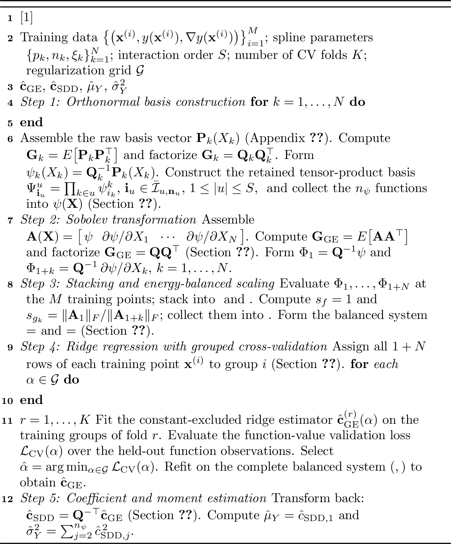
This subsection outlines the computational procedure and the associated cost of constructing the \(S\)-variate GE-SDD surrogate. Figure 1 presents the overall workflow, and Algorithm 2 states the complete procedure at the end of this subsection.
The procedure begins with the input-output-gradient dataset \(\{\mathbf{x}^{(i)},y(\mathbf{x}^{(i)}), \nabla y(\mathbf{x}^{(i)})\}_{i=1}^{M}\). We first construct the \(L^2\)-orthonormal SDD basis \(\boldsymbol{\psi}(\mathbf{X})\) from the prescribed spline parameters through the whitening transformation described in Section 2.4 and Appendix 6. We then assemble the extended basis matrix \(\mathbf{A}(\mathbf{X})\) from the basis and its partial derivatives and factorize the derivative-augmented spline moment matrix \(\mathbf{G}_{\mathrm{GE}}=\mathbf{Q}\mathbf{Q}^\top\), which maps the function value and its gradients into the common Sobolev coordinates \(\boldsymbol{\Phi}_1,\ldots,\boldsymbol{\Phi}_{1+N}\) (Section 3.1).
Because the function-value and derivative blocks generally differ in Frobenius norm, we introduce the block-wise scaling factors \(s_{g_k}=\|\mathbf{A}_1\|_F/\|\mathbf{A}_{1+k}\|_F\) to form the energy-balanced system \((\tilde{\mathbf{A}}_{\mathrm{stack}},\tilde{\mathbf{b}}_{\mathrm{stack}})\), which prevents a high-norm block from dominating the stacked regression loss (Section 3.2). We then estimate the coefficients by constant-excluded ridge regression, selecting \(\hat{\alpha}\) by grouped \(K\)-fold cross-validation that keeps all \(1+N\) observations of each training point in the same fold (Section 3.3). Finally, we map the solution back to the \(L^2\)-orthonormal SDD coordinates (\(\hat{\mathbf{c}}_{\mathrm{SDD}}=\mathbf{Q}^{-\top} \hat{\mathbf{c}}_{\mathrm{GE}}\)), preserving closed-form mean and variance estimates (Section 3.4). The cost is governed by \(n_\psi=L_{S,\mathbf{p},\boldsymbol{\Xi}}\) in 5 and the \(M(1+N)\) stacked equations, with detailed analysis deferred to Section 4.4.
4 Numerical examples↩︎
We evaluate the proposed GE-SDD on three benchmarks of increasing input dimension and complexity: a two-dimensional continuous exponential function in Section 4.1, a two-degree-of-freedom linear dynamical system with three uncertain parameters in Section 4.2, and a 30-dimensional compliance problem for a 25-bar transmission-tower-type space truss in Section 4.3. Unless stated otherwise, all experiments follow the common setup below. Tables report arithmetic means over 20 independent replications, while box plots summarize the distributions and medians. We compare GE-SDD with:
SDD: conventional SDD trained on function values, using the same orthonormal basis, constant-excluded ridge estimator, regularization grid, and \(K\)-fold cross-validation procedure as GE-SDD.
Kriging: Gaussian process regression trained on function values [9]. The model uses a constant trend, affinely scaled inputs, standardized outputs, and anisotropic length scales estimated by maximum likelihood. Example 1 uses a Matérn \(3/2\) kernel with a nugget of \(10^{-10}\) and five random restarts. Examples 2 and 3 use an anisotropic squared-exponential kernel with a nugget of \(10^{-8}\).
GE-Kriging: Gradient-enhanced Kriging based on the exact joint covariance of function values and gradients for the corresponding kernel [9], [21]. GE-Kriging uses the same \(M\) training samples and \(M\times N\) derivative observations as GE-SDD. Each example specifies the hyperparameter-selection strategy.
RBF: A Gaussian radial basis function surrogate, \(\phi(\mathbf{x},\mathbf{x}') =\exp(-\|\mathbf{x}-\mathbf{x}'\|_2^2/d_0^2)\), trained on function values and included only in Example 1. We select the shape parameter \(d_0\) by \(K\)-fold cross-validation over a logarithmically spaced grid. The model uses the same input and output scaling as Kriging, no polynomial tail, and a regularization coefficient of \(10^{-10}\).
We measure surrogate accuracy using the normalized root-mean-square error \(\mathrm{NRMSE} := \frac{\mathrm{RMSE}}{\sigma_{Y,\mathrm{MCS}}} \times 100\%, \label{eq:nrmse}\) where the RMSE is evaluated on a reference MCS sample of size \(M_{\mathrm{MCS}}=10^6\), or the fixed subsample specified for an individual example. The quantity \(\sigma_{Y,\mathrm{MCS}}\) is the corresponding MCS estimate of the output standard deviation. We also report the coefficient of determination \(R^2\) and the mean absolute error (MAE) where relevant.
4.1 Example 1: Two-dimensional continuous exponential function↩︎
The first benchmark is a two-dimensional continuous exponential function with a localized peak at the origin: \[y(x_1,x_2) = \exp\!\bigl(-2|x_1|-2|x_2|\bigr), \qquad x_1,x_2\in[-1,1]. \label{eq:cont-exp}\tag{39}\] The inputs \(X_1\) and \(X_2\) are independent and uniformly distributed on \([-1,1]\). The response decays rapidly from the origin and is continuous but nondifferentiable along the coordinate axes. These localized, nonsmooth features challenge surrogates trained only on function values. Away from the coordinate axes, the partial derivatives are \[\frac{\partial y}{\partial x_k} = -2\,\operatorname{sign}(x_k) \exp\!\bigl(-2|x_1|-2|x_2|\bigr), \qquad k=1,2,\quad x_k\ne0. \label{eq:cont-exp-grad}\tag{40}\] The classical derivative is undefined at \(x_k=0\). We set \(\operatorname{sign}(0)=0\), corresponding to the symmetric subgradient convention at the cusp. Because the training samples follow continuous uniform distributions, the probability of sampling \(x_k=0\) exactly is zero; the adopted convention therefore does not affect the reported random-sampling results.
4.1.0.1 Spline discretization.
SDD and GE-SDD use the same cubic B-spline basis with \(p_k=3\) for \(k=1,2\). Each input coordinate uses the open knot vector \(\boldsymbol{\xi}_k = \bigl( \underbrace{-1,\ldots,-1}_{4},\, -\tfrac{1}{2},\, \underbrace{0,\,0,\,0}_{3},\, \tfrac{1}{2},\, \underbrace{1,\ldots,1}_{4} \bigr), \; k=1,2. \label{eq:example1-knots}\) The interior knots are \(\{-\tfrac{1}{2},0,\tfrac{1}{2}\}\) with multiplicity three at the origin. This repeated knot reduces the interelement continuity of the cubic spline space from \(C^{2}\) to \(C^{3-3}=C^{0}\) at \(x_k=0\), so the univariate spline space can represent a kink exactly at the known location of the nonsmooth ridge of 39 . Both SDD and GE-SDD methods use the same knot vector, so their comparison isolates the effect of gradient observations from that of the approximation space. The knot vector in [eq:example1-knots] generates \(n_k=9\) univariate basis functions per coordinate.
With interaction order \(S=2\), the number of retained basis functions is \(n_\psi = 1+2(9-1)+(9-1)^2 = 81. \label{eq:example1-basis-count}\) Both surrogates use the same \(M=81\) independently drawn training samples. The function-only SDD design matrix is therefore square, with 81 equations and \(81\) coefficients. GE-SDD adds two derivative equations per sample, producing \(3M=243\) stacked equations for the same \(81\) coefficients.
| Method | NRMSE (%) | \(R^2\) |
|---|---|---|
| GE-SDD | 1.022 | 0.9996 |
| SDD | 36.326 | 0.7298 |
| GE-Kriging | 10.238 | 0.9891 |
| Kriging | 8.731 | 0.9922 |
| RBF | 21.138 | 0.9526 |
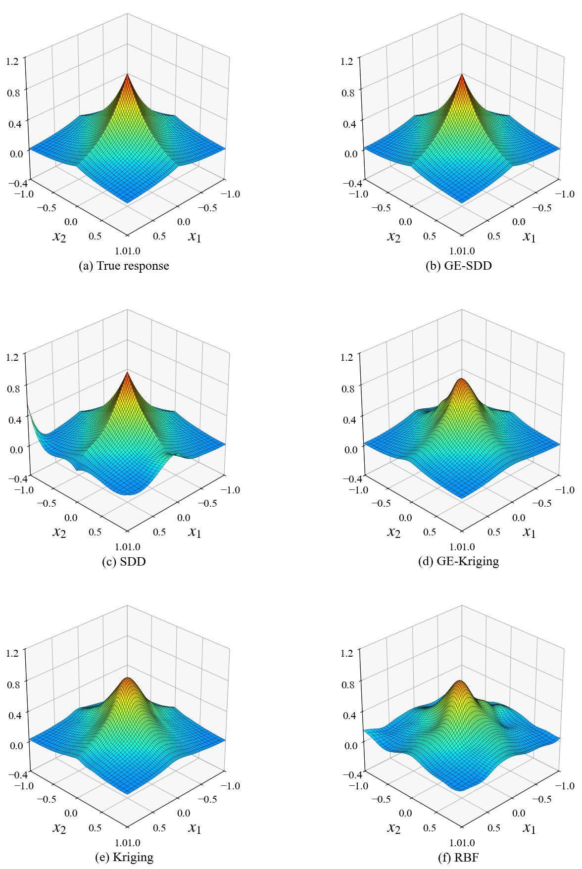
Table 1 reports the mean prediction accuracy over the 20 replications. GE-SDD achieves the lowest mean NRMSE of \(1.022\%\) and the highest mean \(R^2\) of \(0.9996\). Its mean NRMSE is more than eight times lower than that of Kriging (\(8.731\%\)), the most accurate baseline, and more than \(35\) times lower than that of standard SDD (\(36.326\%\)). Function-only Kriging achieves slightly higher accuracy GE-Kriging (\(8.731\%\) versus \(10.238\%\)). One plausible explanation is the mismatch between the Matérn \(3/2\) joint covariance model and the nonsmooth response. The true gradient in 40 changes sign discontinuously across the coordinate axes, whereas the covariance model imposes a smooth joint function–gradient structure. Gradient observations on opposite sides of a cusp may therefore conflict with the assumed covariance. In contrast, the GE-SDD basis admits \(C^0\) continuity at the known cusp locations, allowing the model to use the gradient sign changes directly.
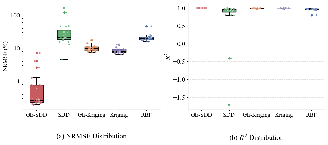
Figure 4 summarizes the variability of the metrics across replications. The median NRMSEs are \(0.269\%\) for GE-SDD, \(21.772\%\) for SDD, \(9.683\%\) for GE-Kriging, \(8.086\%\) for Kriging, and \(19.945\%\) for RBF. GE-SDD achieves an NRMSE below 1% in 15 of the 20 replications. The largest GE-SDD NRMSE of \(7.208\%\) remains below the median Kriging NRMSE. Standard SDD produces NRMSEs ranging from \(4.5\%\) to \(166.6\%\) and negative \(R^2\) values in 2 replications. These results show that the square function-only system is sensitive to the placement of training samples near the localized peak. The derivative constraints substantially reduce this sensitivity.
The response surfaces in Figure 3 support the quantitative results. GE-SDD captures the peak amplitude and rapid decay in Figure 3 (b), whereas standard SDD produces local artifacts near the peak and in sparsely sampled regions in Figure 3 (c). GE-Kriging and Kriging reproduce the reference response away from the origin but smooth the cusps. RBF shows the largest deviations near the peak and the domain boundary.
4.2 Example 2: Two-degree-of-freedom linear dynamical system↩︎
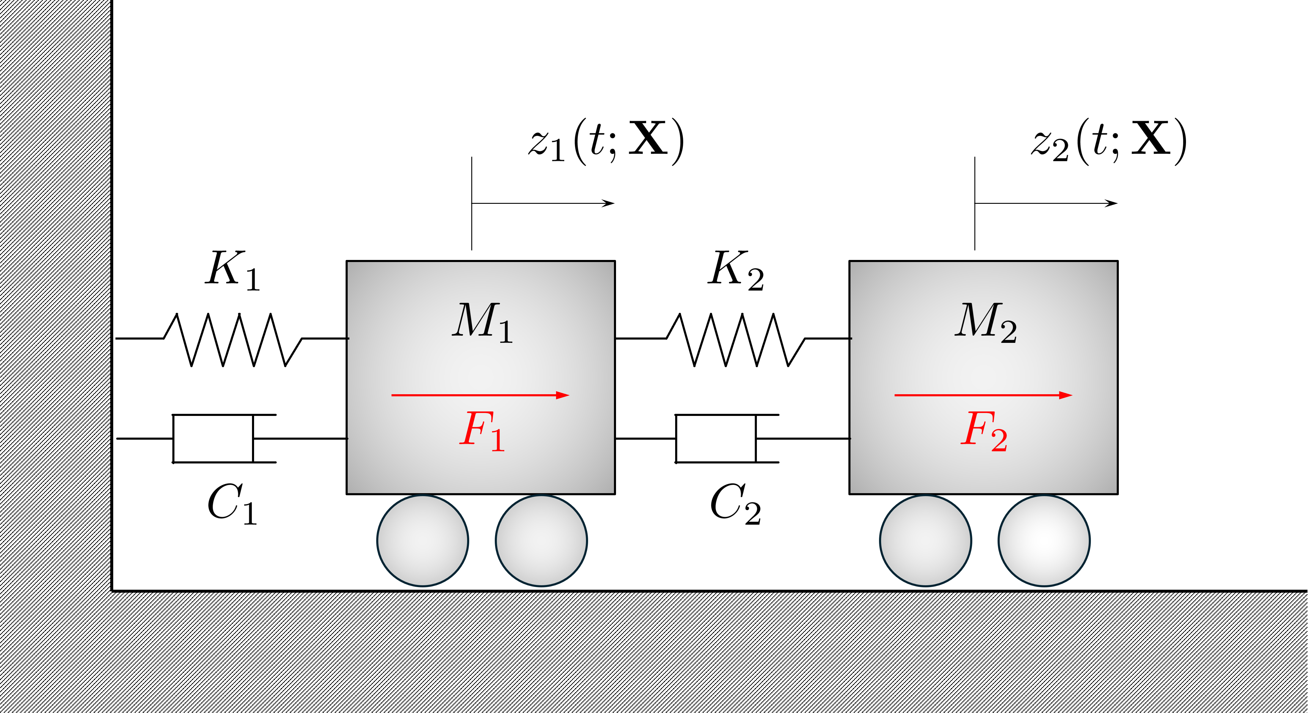
The second benchmark is a two-degree-of-freedom (2-DOF) linear dynamical system with three uncertain structural parameters representing mass, damping, and stiffness. Figure 5 illustrates the system configuration. The spring–damper pair \((K_1,C_1)\) connects mass \(M_1\) to the fixed support, while \((K_2,C_2)\) connects mass \(M_2\) to \(M_1\). The forces \(F_1(t)\) and \(F_2(t)\) act in the positive displacement direction, and \(Z_1(t;\mathbf{X})\) and \(Z_2(t;\mathbf{X})\) denote the displacements.
For excitation frequency \(f\) in Hz, define the angular frequency \(\omega:=2\pi f. \label{eq:angular-frequency}\) The frequency-domain equilibrium equation is \[\mathbf{D}(f;\mathbf{X})\, \mathbf{Z}(f;\mathbf{X}) = \widehat{\mathbf{F}}, \label{eq:2dof-eom}\tag{41}\] where \[\mathbf{D}(f;\mathbf{X}) := -\omega^2 \begin{bmatrix} M_1 & 0\\ 0 & M_2 \end{bmatrix} + \mathrm{i}\omega \begin{bmatrix} C_1+C_2 & -C_2\\ -C_2 & C_2 \end{bmatrix} + \begin{bmatrix} K_1+K_2 & -K_2\\ -K_2 & K_2 \end{bmatrix}, \label{eq:2dof-dynamic-stiffness}\tag{42}\] and \[\mathbf{Z}(f;\mathbf{X}) := \begin{bmatrix} Z_1(f;\mathbf{X})\\ Z_2(f;\mathbf{X}) \end{bmatrix}, \qquad \widehat{\mathbf{F}} := \begin{bmatrix} \widehat F_1\\ \widehat F_2 \end{bmatrix}. \label{eq:2dof-response-force}\tag{43}\]
The uncertain input vector is \[\mathbf{X} := (X_M,X_C,X_K)^\top \in\mathbb{R}^3, \label{eq:2dof-input}\tag{44}\] where \(X_M\), \(X_C\), and \(X_K\) are independent \(U(-3,3)\) random variables. The physical parameters are \[M_1=M_2 = (1+0.05X_M)\;\mathrm{kg}, \qquad C_1=C_2 = (1+0.05X_C)\;\mathrm{N{\cdot}s/m}, \qquad K_1=K_2 = 15000(1+0.05X_K)\;\mathrm{N/m}. \label{eq:2dof-params}\tag{45}\]
We apply a unit harmonic force to \(M_1\), such that \(\widehat{\mathbf{F}} = (1,0)^\top. \label{eq:2dof-numerical-force}\) At each fixed frequency, the surrogate approximates the response magnitude \[y_f(\mathbf{X}) := \left|Z_1(f;\mathbf{X})\right|. \label{eq:2dof-qoi}\tag{46}\] We construct a separate surrogate at each of 100 equally spaced frequencies \(f_j\in[10,35]\;\mathrm{Hz}, \;j=1,\ldots,100.\) The estimated coefficients provide the frequency-dependent standard deviation \[\sigma_{|Z_1|}(f_j) := \sqrt{ \mathbb{V}\mathrm{ar} \left[ |Z_1(f_j;\mathbf{X})| \right] }. \label{eq:2dof-std-curve}\tag{47}\]
4.2.0.1 Analytic response sensitivities.
We compute the GE-SDD gradients by differentiating the complex equilibrium equation. For \(q\in\{X_M,X_C,X_K\}\), differentiation of 41 gives \[\frac{\partial\mathbf{Z}}{\partial q} = -\mathbf{D}^{-1} \frac{\partial\mathbf{D}}{\partial q} \mathbf{Z}, \label{eq:2dof-response-sensitivity}\tag{48}\] because \(\widehat{\mathbf{F}}\) does not depend on the uncertain parameters. The required derivatives are \[\frac{\partial\mathbf{D}}{\partial X_M} = -\omega^2 \left( 0.05\,\mathbf{I}_2 \right), \qquad \frac{\partial\mathbf{D}}{\partial X_C} = \mathrm{i}\omega \begin{bmatrix} 0.10 & -0.05\\ -0.05 & 0.05 \end{bmatrix}, \qquad \frac{\partial\mathbf{D}}{\partial X_K} = \begin{bmatrix} 1500 & -750\\ -750 & 750 \end{bmatrix}. \label{eq:2dof-dD}\tag{49}\] For \(|Z_1|>0\), the response-magnitude derivative is \[\frac{\partial y_f}{\partial q} = \frac{ \operatorname{Re}\!\left[ \overline{Z_1} \dfrac{\partial Z_1}{\partial q} \right] }{ |Z_1| }, \qquad q\in\{X_M,X_C,X_K\}. \label{eq:2dof-magnitude-sensitivity}\tag{50}\] We set the derivative to zero when \(|Z_1|\le10^{-15}\) to avoid division by a near-zero magnitude. Equations 48 –50 define a direct analytical sensitivity calculation rather than an adjoint method.
4.2.0.2 Spline discretization.
SDD and GE-SDD use \(p_k=2\), \(n_k=18\), and maximum interaction order \(S=2\) in all 3 input dimensions. The retained basis contains \[n_\psi = 1+3(18-1)+{3\choose2}(18-1)^2 = 919 \label{eq:2dof-basis-count}\tag{51}\] functions. Each frequency-wise surrogate uses \(M=919\) training samples.
4.2.0.3 Baseline configuration and evaluation.
We train an independent Kriging model at each frequency using all \(M=919\) training samples and estimate its amplitude and anisotropic length scales by maximum likelihood. GE-Kriging uses the same \(MN\) analytical derivative observations through the joint function–gradient covariance. Repeated maximum-likelihood optimization of the \((N+1)M\times(N+1)M\) covariance matrix is impractical across 100 frequencies. We therefore select the GE-Kriging hyperparameters by training-sample-grouped \(K\)-fold cross-validation over a logarithmically spaced grid.
We estimate the Kriging and GE-Kriging standard-deviation curves from predictions on a fixed \(5\times10^4\)-sample subset of the Monte Carlo reference set. SDD and GE-SDD provide the same statistics directly from their coefficients using 37 .
| Method | MAE (\(\times10^{-5}\)) | Rel.err.(%) | \(R^2\) |
|---|---|---|---|
| GE-SDD | 2.435 | 2.45 | 0.977 |
| SDD | 4.978 | 15.95 | 0.387 |
| Kriging | 1.151 | 1.49 | 0.994 |
| GE-Kriging | 4.651 | 5.97 | 0.870 |
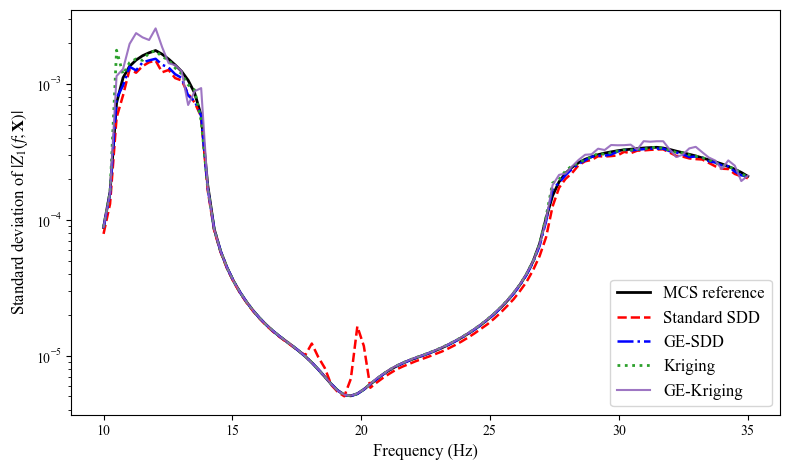
This benchmark tests a frequency-dependent response with strong resonance behavior. Near resonance, small parameter changes shift both the magnitude and location of the response peaks, producing a strongly nonlinear input–output map despite the linear equations of motion. Figure 6 shows that all 4 surrogates agree closely with the reference away from resonance. The main differences occur near the first resonance at approximately \(12\,\mathrm{Hz}\). Standard SDD underestimates the peak, consistent with shrinkage of the nonconstant coefficients under the regularization selected for the square function-only system. GE-Kriging shows the largest local deviations, while GE-SDD and Kriging track the reference closely.
Table 2 reports the mean accuracy over 20 replications. Kriging achieves the lowest mean MAE of \(1.151\times10^{-5}\). GE-SDD follows with \(2.435\times10^{-5}\), GE-Kriging with \(4.651\times10^{-5}\), and standard SDD with \(4.978\times10^{-5}\).
GE-SDD is more accurate and less variable than standard SDD and GE-Kriging in this benchmark. GE-SDD produces a lower MAE than both methods in all 20 replications and reduces the mean relative error of standard SDD from \(15.95\%\) to \(2.45\%\). The coefficient of variation of the GE-SDD MAE is \(9.4\%\), compared with \(20.1\%\) for Kriging, \(34.2\%\) for GE-Kriging, and \(68.3\%\) for standard SDD.
The same gradient observations provide less benefit to GE-Kriging. GE-Kriging is less accurate than function-only Kriging on average, and its least accurate replication produces a curve \(R^2\) of \(0.118\). This result indicates the difficulty of selecting joint-covariance hyperparameters near resonance.
Function-only Kriging remains the most accurate method for this low-dimensional benchmark and achieves approximately half the GE-SDD MAE in every replication. This advantage is consistent with frequency-specific maximum-likelihood adaptation of the anisotropic length scales. Near resonance, the estimated length scales decrease by more than an order of magnitude in the mass and stiffness directions while remaining large in the damping direction. This behavior follows the resonance relation \(\omega_{\mathrm{res}}^2\propto K/M\). The fixed spline basis used by SDD and GE-SDD does not adapt with frequency, so the remaining GE-SDD error concentrates near the first resonance. This result motivates the gradient-guided adaptive knot placement discussed in Section 5.
4.3 Example 3: 30-dimensional 25-bar space truss compliance problem↩︎
The third benchmark is a 30-dimensional compliance problem for a 25-bar transmission-tower-type space truss. Figure 7 illustrates the structural geometry, supports, and loading. The structure contains 10 nodes and 25 members, with nodes 7–10 fully fixed. This benchmark tests SDD and GE-SDD in a high-dimensional, limited-sample regime where the retained basis contains substantially more coefficients than the number of function-value observations.
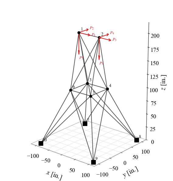
The input random vector is \(\mathbf{X} = (A_1,\ldots,A_{25}, P_1,P_2,P_3,P_4,P_5)^\top \in\mathbb{R}^{30}, \label{eq:truss25-input}\) where \(A_i\), \(i=1,\ldots,25\), denotes the cross-sectional area of the \(i\)-th member. The variables \(P_1\) and \(P_2\) define the \(x\)- and \(y\)-direction loads at node 1, while \(P_3\) and \(P_4\) define the corresponding loads at node 2. The variable \(P_5\) defines the common load in the negative \(z\)-direction at both nodes. All input variables are mutually independent and uniformly distributed. Table 3 lists their bounds.
| Variable | Description | Unit | \(a_k\) | \(b_k\) |
|---|---|---|---|---|
| \(A_1,\ldots,A_{25}\) | member cross-sectional areas | in\(^2\) | 0.5 | 1.5 |
| \(P_1\) | \(x\)-direction load at node 1 | lbf | \(-2.0\times10^{3}\) | \(2.0\times10^{3}\) |
| \(P_2\) | \(y\)-direction load at node 1 | lbf | \(8.0\times10^{3}\) | \(1.2\times10^{4}\) |
| \(P_3\) | \(x\)-direction load at node 2 | lbf | \(-2.0\times10^{3}\) | \(2.0\times10^{3}\) |
| \(P_4\) | \(y\)-direction load at node 2 | lbf | \(8.0\times10^{3}\) | \(1.2\times10^{4}\) |
| \(P_5\) | vertical load at nodes 1 and 2 | lbf | \(-6.0\times10^{3}\) | \(-4.0\times10^{3}\) |
The quantity of interest is the structural compliance \[Y(\mathbf{X}) = C(\mathbf{X}) = \mathbf{F}(\mathbf{X})^\top \mathbf{u}(\mathbf{X}) = \mathbf{F}(\mathbf{X})^\top \mathbf{K}(\mathbf{X})^{-1} \mathbf{F}(\mathbf{X}), \label{eq:truss25-compliance}\tag{52}\] where \(\mathbf{K}(\mathbf{X})\in\mathbb{R}^{18\times18}\), \(\mathbf{F}(\mathbf{X})\in\mathbb{R}^{18}\), and \(\mathbf{u}(\mathbf{X})\in\mathbb{R}^{18}\) denote the assembled global stiffness matrix, nodal load vector, and nodal displacement vector, respectively, defined on the \(18\) free degrees of freedom that remain after eliminating the constrained degrees of freedom at the fixed nodes 7–10 (each of the 10 nodes carries three translational degrees of freedom, and the 12 degrees of freedom at nodes 7–10 are removed). The stiffness matrix depends on the member areas through the linear assembly \(\mathbf{K}(\mathbf{X})=\sum_{j=1}^{25}A_j\mathbf{K}_j\), where \(\mathbf{K}_j\) is the unit-area element stiffness contribution of member \(j\). The load vector \(\mathbf{F}(\mathbf{X})\) collects the uncertain nodal loads \(P_1,\ldots,P_5\): \(P_1\) and \(P_2\) act in the \(x\)- and \(y\)-directions at node 1, \(P_3\) and \(P_4\) act in the \(x\)- and \(y\)-directions at node 2, and \(P_5\) acts in the negative \(z\)-direction at both nodes 1 and 2. The Young’s modulus is fixed at \(E=1.0\times10^7\,\mathrm{psi}\).
4.3.0.1 Analytical compliance sensitivities.
The self-adjoint compliance formulation gives \[\begin{align} \frac{\partial C}{\partial A_j} &= -\mathbf{u}^\top \frac{\partial\mathbf{K}}{\partial A_j} \mathbf{u}, \qquad j=1,\ldots,25, \tag{53} \\ \frac{\partial C}{\partial P_k} &= 2 \left( \frac{\partial\mathbf{F}}{\partial P_k} \right)^\top \mathbf{u}, \qquad k=1,\ldots,5. \tag{54} \end{align}\] These expressions provide all 30 gradients without additional state-equation solutions beyond the displacement analysis used to evaluate the compliance.
4.3.0.2 Spline discretization.
SDD and GE-SDD use quadratic B-splines with \(p_k=2\) and maximum interaction order \(S=2\). The area dimensions use a finer univariate basis than the load dimensions: \[n_k = \begin{cases} 5, & k=1,\ldots,25,\\ 3, & k=26,\ldots,30. \end{cases} \label{eq:truss25-basis-resolution}\tag{55}\]
Accordingly, the 25 area dimensions each contribute four nonconstant univariate basis functions, whereas the five load dimensions each contribute two. The resulting number of retained basis functions is \[\begin{align} n_\psi &= 1 +25(5-1)+5(3-1) +{25\choose2}(5-1)^2 +25\cdot5(5-1)(3-1) +{5\choose2}(3-1)^2 = 5951 \label{eq:truss25-basis-count} \end{align}\tag{56}\] functions.
Standard SDD provides \(M\) function-value equations for estimating the 5951 coefficients. GE-SDD provides one function-value equation and 30 derivative equations per training sample, producing \(31M\) stacked equations. At \(M=100\), standard SDD therefore uses 100 equations, while GE-SDD uses 3100 function-gradient equations at the same 100 input locations. Although both systems remain underdetermined, the gradients provide substantially more information for coefficient estimation.
We test \(M\in\{100,150,200,300,500,1000\} \label{eq:truss-training-sizes}\) and repeat each case over 20 independently generated training sets. The reference statistics and pointwise prediction errors are evaluated using the same MCS sample of size \(10^6\). SDD and GE-SDD estimate the mean and standard deviation directly from their coefficients. Kriging estimates the same quantities from predictions on the MCS sample.
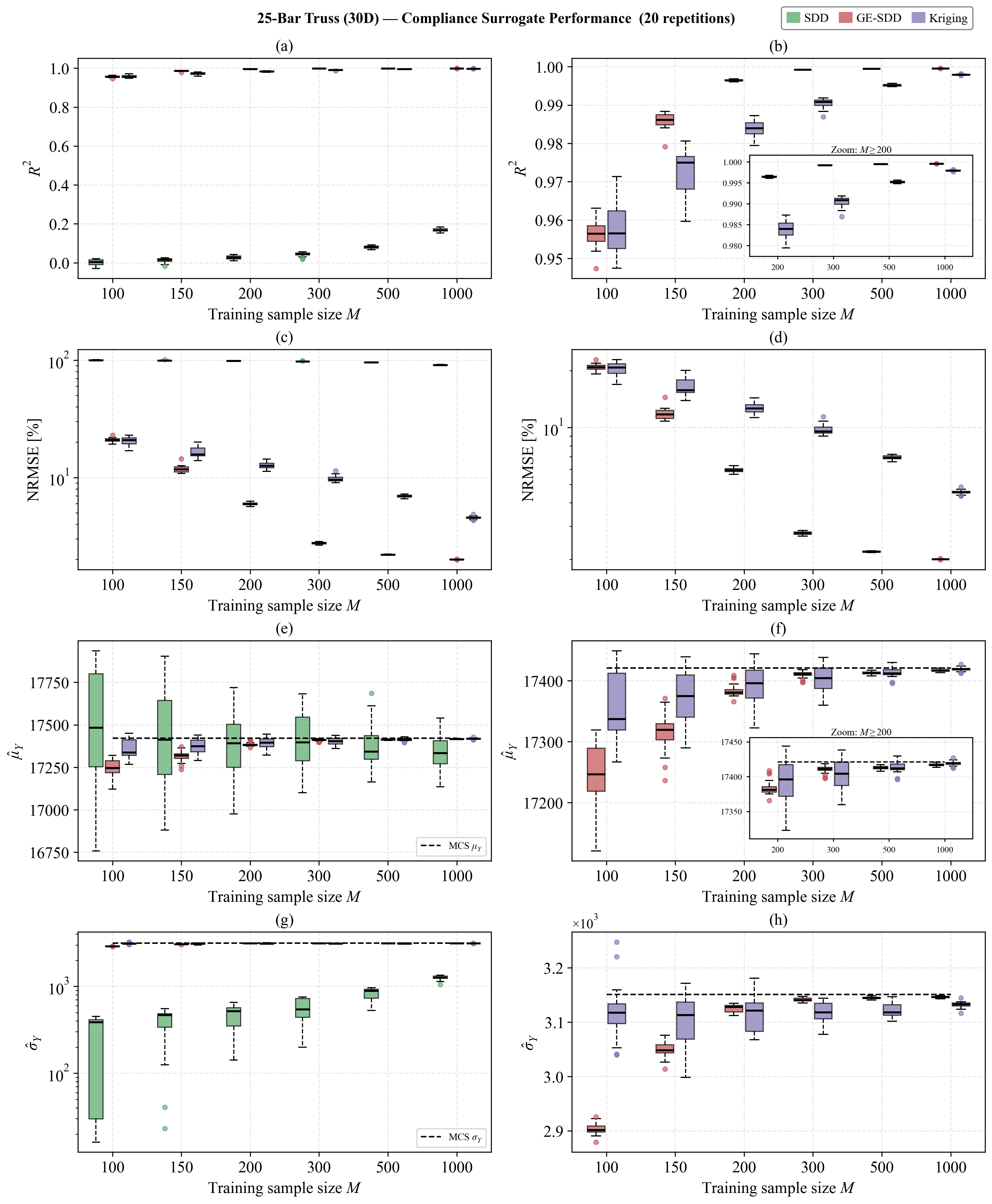
We compare GE-SDD with standard SDD and Kriging. We omit GE-Kriging because the 30-dimensional problem would require training on \(31M\) correlated function and gradient observations. Repeated hyperparameter optimization at this scale is computationally prohibitive for the present training-size sweep. Figure 8 summarizes the variability of the prediction and moment-estimation metrics across replications. Table 4 reports their arithmetic means.
The left column of Figure 8 shows that standard SDD remains inaccurate in pointwise prediction across all training sizes. With only \(M\) function-value equations available for the \(5951\) retained coefficients, grouped cross-validation selects strong regularization. Because the ridge penalty excludes the constant coefficient, SDD estimates the mean with average relative errors between \(0.63\%\) and \(1.59\%\). However, regularization shrinks the nonconstant coefficients and drives the surrogate toward a constant-mean model. Consequently, the average NRMSE of standard SDD decreases only from \(99.90\%\) at \(M=100\) to \(91.19\%\) at \(M=1000\), while its average \(R^2\) increases only from \(0.002\) to \(0.168\). SDD also underestimates the standard deviation, with average relative errors decreasing from \(91.1\%\) to \(60.2\%\).
The accuracy comparison between GE-SDD and Kriging depends on the training size. At \(M=100\), the methods have similar pointwise accuracy. The average NRMSE is \(20.90\%\) for GE-SDD and \(20.58\%\) for Kriging, while the average \(R^2\) is \(0.9563\) and \(0.9574\), respectively. GE-SDD produces the lower NRMSE in 8 of the 20 replications. For every tested size from \(M=150\) onward, GE-SDD achieves the lower NRMSE in all 20 replications. The average NRMSE is \(11.83\%\) for GE-SDD and \(16.61\%\) for Kriging at \(M=150\). At \(M=200\), the corresponding values are \(5.95\%\) and \(12.69\%\). The difference increases for \(M\ge300\). GE-SDD decreases from \(2.76\%\) at \(M=300\) to \(2.01\%\) at \(M=1000\), while Kriging decreases from \(9.76\%\) to \(4.54\%\). At \(M=1000\), the average \(R^2\) reaches \(0.9996\) for GE-SDD and \(0.9979\) for Kriging.
| \(M\) | Method | NRMSE (%, avg) | \(R^2\) (avg) | \(\hat{\mu}_Y\) (avg) | \(\hat{\mu}_Y\) err.(%, avg) | \(\hat{\sigma}_Y\) (avg) | \(\hat{\sigma}_Y\) err.(%, avg) |
|---|---|---|---|---|---|---|---|
| 100 | GE-SDD | 20.90 | 0.9563 | \(1.725\times10^4\) | 0.982 | \(2.904\times10^3\) | 7.833 |
| SDD | 99.90 | 0.002 | \(1.749\times10^4\) | 1.589 | \(2.817\times10^2\) | 91.061 | |
| Kriging | 20.58 | 0.9574 | \(1.736\times10^4\) | 0.400 | \(3.118\times10^3\) | 1.608 | |
| 150 | GE-SDD | 11.83 | 0.9859 | \(1.732\times10^4\) | 0.607 | \(3.050\times10^3\) | 3.193 |
| SDD | 99.38 | 0.012 | \(1.743\times10^4\) | 1.410 | \(3.887\times10^2\) | 87.664 | |
| Kriging | 16.61 | 0.9721 | \(1.737\times10^4\) | 0.287 | \(3.103\times10^3\) | 1.592 | |
| 200 | GE-SDD | 5.95 | 0.9965 | \(1.738\times10^4\) | 0.213 | \(3.125\times10^3\) | 0.817 |
| SDD | 98.69 | 0.026 | \(1.736\times10^4\) | 0.946 | \(4.488\times10^2\) | 85.755 | |
| Kriging | 12.69 | 0.9838 | \(1.739\times10^4\) | 0.186 | \(3.114\times10^3\) | 1.277 | |
| 300 | GE-SDD | 2.76 | 0.9992 | \(1.741\times10^4\) | 0.064 | \(3.141\times10^3\) | 0.306 |
| SDD | 97.80 | 0.043 | \(1.740\times10^4\) | 0.784 | \(5.496\times10^2\) | 82.557 | |
| Kriging | 9.76 | 0.9904 | \(1.741\times10^4\) | 0.124 | \(3.118\times10^3\) | 1.033 | |
| 500 | GE-SDD | 2.20 | 0.9995 | \(1.741\times10^4\) | 0.047 | \(3.144\times10^3\) | 0.209 |
| SDD | 95.84 | 0.081 | \(1.737\times10^4\) | 0.693 | \(8.309\times10^2\) | 73.631 | |
| Kriging | 6.92 | 0.9952 | \(1.741\times10^4\) | 0.054 | \(3.122\times10^3\) | 0.922 | |
| 1000 | GE-SDD | 2.01 | 0.9996 | \(1.742\times10^4\) | 0.025 | \(3.146\times10^3\) | 0.155 |
| SDD | 91.19 | 0.168 | \(1.733\times10^4\) | 0.627 | \(1.255\times10^3\) | 60.179 | |
| Kriging | 4.54 | 0.9979 | \(1.742\times10^4\) | 0.019 | \(3.132\times10^3\) | 0.600 |
The right column of Figure 8 shows that GE-SDD variability decreases rapidly as \(M\) increases. The across-replication standard deviation of the GE-SDD NRMSE decreases from \(0.80\) percentage points at \(M=100\) to less than \(0.01\) percentage points at \(M=1000\). Kriging has greater variability at every tested training size.
The moment estimates show a similar training-size transition. Both methods estimate the mean accurately throughout the sweep. Kriging has lower average relative mean errors for \(M\le200\). At \(M=100\), \(150\), and \(200\), the Kriging errors are \(0.400\%\), \(0.287\%\), and \(0.186\%\), compared with \(0.982\%\), \(0.607\%\), and \(0.213\%\) for GE-SDD. The methods produce similar mean estimates for \(M\ge300\), and both average relative errors fall below \(0.03\%\) at \(M=1000\).
Kriging also estimates the standard deviation more accurately at \(M=100\) and \(150\). GE-SDD becomes more accurate for \(M\ge200\). At \(M=1000\), the average relative standard-deviation error is \(0.155\%\) for GE-SDD and \(0.600\%\) for Kriging. Thus, gradient observations provide no clear advantage at the smallest training size, where \(31M\) remains well below the 5951 retained coefficients. From \(M=150\) onward, GE-SDD provides more accurate pointwise predictions, and from approximately \(M=200\) onward, it provides more accurate standard-deviation estimates.
4.4 Discussion↩︎
GE-SDD uses \(M\) function observations and \(M\times N\) partial-derivative observations. The number of distinct input locations therefore remains \(M\), but the cost of obtaining the gradients depends on the underlying model. Example 1 provides explicit derivatives. In Example 2, direct sensitivity analysis requires additional linear-system solutions for the three uncertain parameters, but all solutions reuse the same dynamic-stiffness factorization. In Example 3, the self-adjoint compliance formulas require no additional state-equation solutions. For more general applications, adjoint sensitivity analysis or automatic differentiation can reduce the marginal cost of gradient observations relative to additional high-fidelity simulations.
The algebraic cost of GE-SDD depends primarily on the retained basis size \(n_\psi=L_{S,\mathbf{p},\boldsymbol{\Xi}}\) and the \(M(1+N)\) stacked equations. A dense Cholesky factorization of the derivative-augmented spline monomial moment matrix has computational complexity \(\mathcal{O}(n_\psi^3)\). Consequently, the cost increases with input dimension, interaction order, and basis resolution. Large-scale applications can reduce them through sparse linear algebra, iterative solvers, dimension-adaptive basis selection, and further use of the tensor-product and ANOVA structures.
The accuracy gains reported in Table 1, Table 2, and Table 4 depend on the benchmark, training budget, basis resolution, and gradient availability. Example 3 shows that gradient augmentation does not guarantee greater accuracy at every training size. GE-SDD and Kriging have similar pointwise accuracy at \(M=100\). GE-SDD becomes more accurate at \(M\ge150\), and the difference increases at \(M\ge300\).
The three benchmarks show when gradient augmentation is most beneficial. In Example 2 with \(N=3\) and \(M=919\), Kriging remains the most accurate method because it re-estimates the anisotropic length scales at each frequency. GE-SDD is most accurate for the nonsmooth response in Example 1 and for the high-dimensional problem in Example 3 at moderate and large training sizes. In these settings, case-specific maximum-likelihood adaptation is less effective or computationally impractical. The observed crossover training sizes are not universal; they depend on the retained basis size, regularization, response structure, and the accuracy and cost of the gradients. Further studies using large-scale finite-element and computational fluid dynamics models with solver-based sensitivities are needed to assess the broader accuracy and computational efficiency of GE-SDD.
5 Conclusions↩︎
This paper proposed a gradient-enhanced spline dimensional decomposition (GE-SDD) method for uncertainty quantification (UQ) with limited training samples, including high-dimensional regimes. GE-SDD combines function values and partial derivatives through a probability-weighted Sobolev transformation, balances the function and derivative blocks, and estimates the coefficients using ridge regression with training-sample-grouped \(K\)-fold cross-validation. A final coefficient-estimation step transforms the solution to the original \(L^2\)-orthonormal SDD coordinates, preserving closed-form mean and variance estimates.
Numerical results from three benchmark problems showed that GE-SDD is more accurate than standard SDD and GE-Kriging, while its comparison with function-only Kriging depends on the problem. For the two-dimensional continuous exponential function, GE-SDD achieved a median NRMSE of \(0.269\%\), compared with \(8.086\%\) for Kriging, the most accurate baseline in that benchmark. For the 2-DOF dynamical system, GE-SDD reduced the MAE of the predicted frequency-dependent standard deviation to \(2.435\times10^{-5}\), compared with \(4.978\times10^{-5}\) for standard SDD and \(4.651\times10^{-5}\) for GE-Kriging. GE-SDD was more accurate than both in every replication with the smallest across-replication variability; the frequency-wise maximum-likelihood-tuned Kriging baseline attained the lowest MAE of \(1.151\times10^{-5}\) in this low-dimensional benchmark. For the 30-dimensional truss, GE-SDD and Kriging had similar pointwise accuracy at \(M=100\). GE-SDD produced lower NRMSE and higher \(R^2\) for \(M\ge150\), with a larger difference at moderate and large training sizes.
The truss results also showed that the relative accuracy depended on the target UQ quantity. Both methods estimated the mean accurately across all training sizes, although Kriging was slightly more accurate at smaller sizes. GE-SDD provided more accurate standard-deviation estimates for \(M\ge200\). Conversely, Example 2 showed that anisotropic Kriging could remain more accurate near sharp resonances when the input dimension was small and frequency-specific hyperparameter optimization was computationally feasible. The benefits of gradient augmentation therefore depended on the input dimension, training size, basis resolution, response structure, and target statistic.
Future work will evaluate GE-SDD on large-scale finite-element and computational fluid dynamics models using adjoint sensitivities or automatic differentiation. Further developments will integrate GE-SDD with first- and second-order reliability methods, introduce gradient-guided adaptive knot placement, and develop dimension-adaptive basis selection for responses with localized rapid variations such as resonance zones.
Funding↩︎
This work was supported by the National Research Foundation of Korea (NRF) grant funded by the Korea government (MSIT) (RS-2025-00560781).
Declaration of generative AI and AI-assisted technologies in the writing process↩︎
During the preparation of this work, the authors used OpenAI’s ChatGPT and Anthropic’s Claude for English-language editing, grammar checking, wording refinement, and stylistic polishing. After using these tools, the authors reviewed and edited the content as needed and take full responsibility for the content of the published article.
6 Construction of measure-consistent orthonormal B-spline basis functions↩︎
This appendix presents the detailed construction of the measure-consistent orthonormal B-spline basis functions used in the SDD representation.
Specify the univariate spline spaces. For each input coordinate \(X_k\), let \(p_k\), \(\boldsymbol{\xi}_k\), and \(n_k\) denote the B-spline degree, open knot vector, and number of basis functions, respectively. Collect these parameters as \[\mathbf{p}:=(p_1,\ldots,p_N), \qquad \mathbf{n}:=(n_1,\ldots,n_N), \qquad \boldsymbol{\Xi} := (\boldsymbol{\xi}_1,\ldots,\boldsymbol{\xi}_N). \label{eq:spline-parameter-collections}\tag{57}\] For \(u\subseteq\{1,\ldots,N\}\), let \(\mathbf{p}_u\), \(\mathbf{n}_u\), and \(\boldsymbol{\Xi}_u\) denote the corresponding subcollections.
Construct the raw univariate bases. For the \(k\)-th input coordinate, define \[\mathbf{P}_k(X_k) := \bigl( 1,\, B^k_{2,p_k,\boldsymbol{\xi}_k}(X_k),\, \ldots,\, B^k_{n_k,p_k,\boldsymbol{\xi}_k}(X_k) \bigr)^\top, \label{eq:Pvec}\tag{58}\] \(B^k_{i,p_k,\boldsymbol{\xi}_k}\) is the \(i\)-th B-spline of degree \(p_k\), generated by the Cox–de Boor recursion [28], [29]. Replacing the first B-spline with \(1\) preserves the constant direction during orthonormalization and produces nonconstant basis functions with zero mean under \(f_{X_k}(\mathbf{X}_k)\).
Orthonormalize the univariate bases. Define the Gram matrix \[\mathbf{G}_k := \mathbb{E}\!\left[ \mathbf{P}_k(X_k)\mathbf{P}_k^\top(X_k) \right] = \int_{a_k}^{b_k} \mathbf{P}_k(x)\mathbf{P}_k^\top(x) f_{X_k}(x)\,\mathrm{d}x \in\mathbb{R}^{n_k\times n_k}. \label{eq:gram}\tag{59}\] We evaluate this integral over each nonzero knot span using 24-point Gauss–Legendre quadrature. We use the same rule for the basis-derivative products required by GE-SDD. Because \(\mathbf{G}_k\) is symmetric positive definite, its Cholesky factorization is \(\mathbf{G}_k= \mathbf{Q}_k\mathbf{Q}_k^\top, \label{eq:gram-cholesky-univariate}\) where \(\mathbf{Q}_k\) is nonsingular and lower triangular. The measure-consistent orthonormal basis is \[\boldsymbol{\psi}_k(X_k) := \mathbf{Q}_k^{-1}\mathbf{P}_k(X_k) = \left( \psi^k_{1,p_k,\boldsymbol{\xi}_k}(X_k), \ldots, \psi^k_{n_k,p_k,\boldsymbol{\xi}_k}(X_k) \right)^\top. \label{eq:ortho-univariate}\tag{60}\] This basis satisfies \(\mathbb{E}[\boldsymbol{\psi}_k(X_k)] =(1,0,\ldots,0)^\top, ~\text{and}~ \mathbb{E}\left[ \boldsymbol{\psi}_k(X_k) \boldsymbol{\psi}_k^\top(X_k) \right]= \mathbf{I}_{n_k}. \label{eq:ortho-char}\) Thus, \(\psi^k_{1,p_k,\boldsymbol{\xi}_k}\equiv1\), whereas \(\mathbb{E}\left[ \psi^k_{i,p_k,\boldsymbol{\xi}_k}(X_k) \right]= 0, ~ i=2,\ldots,n_k. \label{eq:univariate-zero-mean}\)
Form the tensor-product bases. For a non-empty interaction subset \[u=\{k_1,\ldots,k_{|u|}\} \subseteq\{1,\ldots,N\},\] define the full multi-index set \[\mathcal{I}_{u,\mathbf{n}_u} := \left\{ \mathbf{i}_u= (i_{k_1}, \dots, i_{k_{|u|}}) : 1\le i_k\le n_k,\; k\in u \right\}. \label{eq:full-index-set}\tag{61}\] For \(\mathbf{i}_u\in\mathcal{I}_{u,\mathbf{n}_u}\), the corresponding tensor-product basis function is \[\Psi^u_{\mathbf{i}_u,\mathbf{p}_u,\boldsymbol{\Xi}_u} (\mathbf{x}_u) := \prod_{k\in u} \psi^k_{i_k,p_k,\boldsymbol{\xi}_k}(x_k). \label{eq:tp-basis-appendix}\tag{62}\]
The full index set in 61 includes the constant index \(i_k=1\). If one or more active coordinates take this constant index, the corresponding tensor-product basis function effectively reduces to a lower-order interaction. Therefore, to prevent the degree of interaction from falling below \(|u|\), the retained SDD basis excludes the constant index in every active coordinate.