Gate-Zero Growth: A Geometric Framework
for Function-Preserving Continual Learning
July 16, 2026
Abstract
We introduce gate-zero growth, a function-preserving (FP) operator for continual learning that adds new residual blocks through a zero-initialised gate. Under a transversality condition, gate-zero growth induces rank separation in the functional Jacobian: old directions are unchanged, new-weight directions are exactly flat at the growth point, and new gate directions are the only first-order source of new functional variation. As gates open during continual learning, function drift is \(O(\|\boldsymbol{\alpha}\|^2)\) and Jacobian leakage \(O(\|\boldsymbol{\alpha}\|_\infty)\), giving a controlled departure from the FP locus. On a \(300\mathrm{M}\to857\mathrm{M}\) Transformer adapted from WikiText-103 to BookCorpus, gate-zero growth reaches near-zero old-domain forgetting (\(\Delta_A < 0.1\)) under both exact-preservation (Isolation) and joint-frontier (Freeze-Nothing) operating points, while a non-FP control (\(G_{\text{stack}}\)) suffers an order-of-magnitude larger forgetting under the same recipe. The same geometric analysis covers LoRA, ReZero, and zero-init adapter constructions, establishing gate-zero growth as the canonical instance of a shared local geometry that governs safe capacity activation in CL.
1 Introduction↩︎
The dominant paradigm for obtaining a more capable language model is to train a larger model from scratch. Model growth — expanding an existing trained model by adding parameters — offers a compelling alternative, provided the grown model can be fine-tuned without forgetting what the smaller model knew. Function-preserving (FP) growth methods [1], [2] satisfy preservation at growth time by construction, but the geometric structure this initialisation creates in parameter space, and why certain continual learning (CL) strategies work better than others on the grown model, has remained unclear.
A wide range of seemingly different methods share a single structural property: gate-zero residual growth, ReZero-style residual scaling [3], LoRA [4] with \(B = 0\) at initialisation, and near-identity / zero-init adapter modules [5] all add new parameters through an additive branch whose contribution factors through a zero- or near-zero-initialised gate. Each of these methods has its own justification and its own preferred CL recipe; their continual-learning behaviour is typically explained operationally rather than through the geometry of the underlying construction. The recurring empirical pattern — that freezing old parameters and training only the new ones recovers preservation at growth time — has not been tied to a formal property that the constructions share.
We argue that the relevant property is geometric. At a zero-initialised gate, the new-weight contribution to the functional Jacobian is exactly zero by the chain rule, with structural consequences for CL geometry that the literature has not derived as a unified system. Under a transversality condition, the post-growth Jacobian decomposes cleanly into the unmodified old block plus up to \(K\) new-gate directions; the Fisher information matrix has a sparse new-weight block; coordinate isolation becomes an exact projection onto a known local subspace; and as gates open during CL, the departure from this structure is locally controlled by polynomial bounds in the gate magnitude. We instantiate this geometry as gate-zero growth, a function-preserving depth operator for continual learning; the same analysis applies to LoRA, ReZero, and zero-init adapter constructions, establishing gate-zero growth as the canonical instance of the shared template.
We instantiate the framework with gate-zero Transformer depth growth and evaluate sequential adaptation from WikiText-103 [6] to BookCorpus [7] at \(300\mathrm{M}\to857\mathrm{M}\) scale. Under the Isolation protocol, gate-zero growth reaches near-zero old-domain forgetting; zero-init residual stacking under the same protocol reaches the same regime (\(\Delta_A < 0.1\) for both), directly validating the framework’s unification claim. A non-FP baseline (\(G_{\text{stack}}\), used as a diagnostic negative control) suffers order-of-magnitude larger forgetting under the same recipe — the rank-separation guarantee fails without zero-init gating. Ablations also reveal that the framework predicts the safest projection point, while a slightly looser point in the same family (soft preservation without weight freezing) strictly dominates full Isolation on the joint \((\mathrm{PPL}_A, \mathrm{PPL}_B)\) frontier — a controlled-departure regime within the local theory.
1.0.0.1 Contributions.
Gate-zero growth. We propose gate-zero growth, an FP operator that adds residual blocks through a zero-initialised gate, achieving exact function preservation at growth and \(\Delta_A < 0.1\) under continual learning at \(300\mathrm{M}\to 857\mathrm{M}\) scale. We recommend two operating points: Isolation (exact preservation, \(\Delta_A = +0.04\)) and Freeze-Nothing (joint \((\mathrm{PPL}_A, \mathrm{PPL}_B)\) optimum, \(\Delta_A = -1.98\)).
Geometric framework. Under a transversality condition, gate-zero growth induces rank separation, sparse-Fisher block structure (Theorem 1, Prop. 5), exact coordinate-projection isolation (Prop. 6), and bounded gate-driven departure (Props. 9, 10). The same analysis covers LoRA, ReZero, and zero-init adapters (Remark 4), establishing gate-zero growth as the canonical instance.
Predictive structural validation. Three falsifiable predictions verified empirically: (a) coordinate freezing is exactly preserving only under FP growth (\(G_{\text{stack}}{+}\)Iso is structurally undefined); (b) LoRA-CL admits no Isolation row because its frozen-base construction is structurally already Isolation; (c) \(\Delta_A < 0.1\) for every zero-init FP operator we test under Isolation. The MoE plasticity gap is mechanistically localised to clone-block redundancy.
2 Related Work↩︎
2.0.0.1 Neural network growth.
Net2Net [1], bert2BERT [2], and LiGO [8] introduce FP / near-FP expansions but provide no functional-Jacobian / rank analysis or CL framing. ReZero-style residual scaling [3], near-identity / zero-init adapters [5], and zero-initialised residual stacking achieve FP (or near-FP) at growth via additive branches with zero- or near-zero-initialised contribution. We propose gate-zero growth for FP depth expansion in CL, and provide the unified rank-separation / functional-Jacobian / sparse-Fisher analysis (Theorem 1, Props. 5, 7; Remark 4) that covers gate-zero growth alongside LoRA, ReZero, and zero-init adapter constructions. \(G_{\text{stack}}\) [9] serves as a non-FP negative control: it duplicates blocks without zero-init gating, so the rank-separation guarantee fails by construction.
2.0.0.2 Parameter-efficient CL.
LoRA [4] and adapter-based approaches [5], [10], [11] with zero-initialised branches satisfy the same zero-init structural property as gate-zero growth (cf.Remark 4); recent continual-LoRA / continual-adapter methods provide alternative low-trainable-budget CL recipes orthogonal to the growth-vs-no-growth axis we study.
2.0.0.3 Continual learning.
Catastrophic forgetting [12], [13] has motivated a long line of regularization-, replay-, and architecture-based methods [14]: EWC [15] and its successors penalize parameter drift via the Fisher information; PackNet [16] uses hard binary masks; Progressive Networks [10] allocate disjoint columns per task; LwF [17] uses output-space distillation; experience replay [18] revisits old data; A-GEM and related gradient-projection methods [19], [20] project task gradients onto the orthogonal complement of past-task gradients; and parameter-efficient CL via LoRA-style adapters [11] updates a low-rank subspace per task. We unify and rank these methods geometrically and focus on the structural geometry of the growth operator rather than the regularizer-design space; direct head-to-head comparison with gradient-projection and adapter-based CL on multi-task sequences is left as future work.
2.0.0.4 Loss landscape geometry.
Fisher information geometry [21] provides the Riemannian foundation for our Fisher-based analysis of preservation constraints (Section 3). Functional-Jacobian analyses in the linearised neural-tangent regime [22] are adjacent in motivation; we work directly in parameter space at the growth point rather than in the infinite-width NTK limit.
3 Theoretical Framework↩︎
We work with a residual architecture in which each block contributes \(\alpha_\ell \cdot \mathrm{Block}_\ell(x)\) to the residual stream, gated by a scalar \(\alpha_\ell\). Growth inserts \(K\) new blocks with gates initialized to \(\alpha_0\) (typically zero); the existing \(r\) “old” blocks are unmodified at growth time.
3.0.0.1 Setup.
Let \(f_{\theta_{\mathrm{old}}}: \mathbb{R}^d \to \mathbb{R}^V\) denote the pre-growth function and \(f_{\theta_{\mathrm{new}}}\) the post-growth function with \(K\) inserted gated blocks. With \(\alpha_0 = 0\), by direct computation \(f_{\theta_{\mathrm{new}}}(x) = f_{\theta_{\mathrm{old}}}(x)\) for all \(x\) — the new blocks are identity through residual addition. Let \(J(\theta) = \nabla_\theta f_\theta(x)\) denote the functional Jacobian.
3.0.0.2 FP locus.
- Let $(f^*) = {’
- f_{’} = f^*}$ with \(f^* = f_{\theta_{\mathrm{old}}}\). The gate-zero growth point \(\theta' = \iota(\theta_{\mathrm{old}})\) lies on \(\mathcal{M}(f^*)\) with \(\mathbb{R}^{K\cdot P_W} \subseteq T_{\theta'}\mathcal{M}(f^*)\) (Theorem 1 (1)); motion along \(T^{\perp}_{\mathrm{new}}\) leaves \(\mathcal{M}(f^*)\) at first order (Prop. 9).
Theorem 1 (Rank separation under transversality). Let \(J_\alpha \in \mathbb{R}^{D \times K}\) (with \(D = \dim f\) the flattened output dimension) collect the \(K\) new-gate Jacobian columns, \(\partial f / \partial \alpha_\ell = \mathrm{Block}_\ell(x; W_\ell)\), and let \(P_{\mathrm{old}}\) denote the orthogonal projection onto \(\mathrm{im}(J(\theta_{\mathrm{old}}))\). Then at the gate-zero growth point \(\theta'\):
(Exact flat directions, unconditional.) The \(K \cdot P_W\) new-weight directions are exactly flat: \(\partial f / \partial W'_\ell = 0\) for all \(\ell\) and all \(x\).
(Conditional rank additivity.) The Jacobian rank satisfies \[\mathrm{rank}(J(\theta')) \;=\; r \;+\; \mathrm{rank}\!\big((I - P_{\mathrm{old}})\, J_\alpha\big) \;\leq\; r + K,\] with equality \(r + K\) iff the projected gate columns \((I - P_{\mathrm{old}})\, J_\alpha\) are linearly independent (transversality). Generic non-degeneracy of the cloned new-block functions \(\mathrm{Block}_\ell\) implies transversality almost surely under small clone noise; degenerate cases (e.g. a block whose output already lies in \(\mathrm{im}(J(\theta_{\mathrm{old}}))\)) violate it.
By contrast, \(G_{\text{stack}}\) does not preserve \(J(\theta_{\mathrm{old}})\) at the growth point because duplicated blocks immediately alter the active old-block computation, so the equivalent rank decomposition is unavailable.
Proof in Appendix 8. Load-bearing content: Part (2)’s conditional rank additivity, the unification across zero-init constructions (Remark 4), and the direct transversality diagnostic (\(\sigma_{\min}^{\perp} = 144.6\), smallest principal angle \(56.9^\circ\); Appendix 9).
Remark 2. The transversality assumption is generic but not vacuous. Theorem 3.1 should be read as a structural statement: gate-zero growth is the enabling construction* for clean rank decomposition, but empirical realisation depends on the cloned-block functions \(\mathrm{Block}_\ell\) being non-degenerate. Function preservation itself is verified directly by max-logit checks (Section 5.1: max logit difference \(0.0\) at \(\alpha_0 = 0\) on real data). We also directly verify transversality by computing the projected-rank residual \((I - P_{\mathrm{old}}) J_\alpha\) at the post-growth Gate-FP checkpoint (\(K = 36\), growth factor \(g = 4\)) with \(M = 200\) random old-direction Jacobian samples (full diagnostic in Appendix 9). The residual is full-rank (\(\sigma_{\min}^{\perp} = 144.6\), condition number \(6.87\)) and the smallest principal angle between \(\mathrm{im}(J_\alpha)\) and the sampled \(\mathrm{im}(J_{\mathrm{old}})\) is \(56.9^\circ\) (largest: \(83.7^\circ\)). Transversality is therefore not merely “generic almost surely” but quantitatively well-separated at the trained checkpoint. A formal genericity argument (the set of noise realisations producing dependence is Lebesgue-zero in \(\mathbb{R}^{K\cdot P_W}\)) is given in Appendix 8, Remark 8.*
Remark 3 (Why rank separation matters). Rank separation is what distinguishes exact* FP from “good initialisation.” Any smooth initialisation can produce a model close to \(f^*\) in function space; gate-zero growth (and structurally analogous zero-init constructions; see Remark 4) additionally guarantees that the functional Jacobian exactly decomposes into an unchanged old block and an additive new block. This structural guarantee is what makes isolation-based CL exact at the growth point rather than approximate.*
Remark 4 (Scope beyond gated residual blocks). Theorem 1 requires two structural properties: (a) the old forward pass is preserved exactly at \(\theta'\), and (b) every new contribution to \(f\) factors through a zero-initialised parameter producing an additive scalar-times-feature term. Any growth operator satisfying both inherits the conclusion. LoRA* with \(\Delta W = BA\), \(B = 0\): \(B\) plays the gate, \(A\) the cloned feature, and transversality reduces to projected \(A\)-induced directions being independent of \(\mathrm{im}(J_{\mathrm{old}})\), which holds generically. Net2Net / zero-init residual stacking zeroes new-block output projections instead of using a scalar gate; the analysis is identical. ReZero [3] satisfies both properties by construction; adapter modules [5] satisfy them exactly under zero-init up-projection variants and approximately under the near-identity init of the original. \(G_{\text{stack}}\) [9] satisfies neither.*
Proposition 5 (Sparse Fisher block structure). Let \(F(\theta') = \mathbb{E}_{x \sim \mathcal{D}}\!\big[J(\theta';x)^\top J(\theta';x)\big]\) be the empirical Fisher information matrix at the gate-zero growth point. Then unconditionally:
The new-weight Fisher block \(F_{W',W'}\) is identically zero;
All cross-terms \(F_{\theta_{\mathrm{old}},W'}\) and \(F_{\alpha,W'}\) involving new weights are identically zero.
The old–gate cross-block \(F_{\theta_{\mathrm{old}},\alpha}\) is generically non-zero, so \(F(\theta')\) is not* block-diagonal between old and new parameters.*
Proof. Both claims follow from Theorem 1 (1): \(\partial f / \partial W'_\ell = 0\) identically at \(\theta'\), so any inner product involving a new-weight Jacobian column with any other column is zero. Old–gate cross-terms involve \(\langle J_{\theta_{\mathrm{old}},j},\, J_{\alpha,k} \rangle\), neither of which vanishes generically. ◻
Proposition 5 has direct CL implications: second-order methods like EWC place no penalty on new-weight movement (the diagonal Fisher entries on \(W'\) are zero), so EWC reduces to gate-only regularisation. Isolation is therefore a coordinate hard constraint, not a consequence of full Fisher orthogonality, as the next proposition formalises.
Proposition 6 (Isolation as a coordinate-subspace projection). Freezing all old parameters during CL on \(\mathcal{D}_B\) gives an exact coordinate projection onto the new-parameter subspace \(T_{\mathrm{new}}= \{0\}^{P_{\mathrm{old}}} \times \mathbb{R}^{P_{\mathrm{new}}}\). At the gate-zero growth point, \(T_{\mathrm{new}}\) decomposes orthogonally into the \(K \cdot P_W\) exactly-flat new-weight directions (\(T_{\mathrm{new}}^{\parallel}\)) and the \(K\) gate directions (\(T_{\mathrm{new}}^{\perp}\)); the former preserve \(f\) for any update magnitude, while the latter activate new function change as soon as gates leave zero. Isolation therefore preserves old parameters exactly, but preservation of the old function during CL still depends on the KL/replay objective once gates open. Under \(G_{\text{stack}}\), the new- and old-coordinate subspaces are not aligned with the FP locus at \(\theta'\) to begin with, so the same coordinate freeze is only an approximate preservation projection.
Proposition 7 (Four-way subspace partition). At \(\theta' = \iota(\theta_{\mathrm{old}})\) under gate-zero growth, the ambient parameter space partitions orthogonally (Euclidean coordinate metric) into four subspaces: \(T_{\mathrm{old}}^{\parallel}\) (old-direction tangents to \(\mathcal{M}(f^*)\), dimension \(\mathrm{nul}(J(\theta_{\mathrm{old}}))\)), \(T_{\mathrm{old}}^{\perp}\) (old-direction normals, dimension \(r\)), \(T_{\mathrm{new}}^{\parallel}\) (exactly flat new-weight directions, dimension \(K \cdot P_W\), contained in \(\ker J(\theta')\)), and \(T_{\mathrm{new}}^{\perp}\) (non-flat new-gate directions, dimension \(K\)). Isolation restricts updates to \(T_{\mathrm{new}}^{\parallel} \oplus T_{\mathrm{new}}^{\perp}\). Under transversality, \(J_\alpha(T_{\mathrm{new}}^{\perp}) \cap \mathrm{im}(J(\theta_{\mathrm{old}})) = \{0\}\), with the smallest principal angle bounded below by the transversality singular value \(\sigma_{\min}^{\perp} := \sigma_{\min}((I - P_{\mathrm{old}}) J_\alpha) > 0\). The new functional capacity per unit gate motion is bounded between \(\sigma_{\min}^{\perp}\) and \(\sigma_{\max}^{\perp}\), so \(\sigma_{\min}^{\perp}\) quantifies plasticity and small \(\sigma_{\min}^{\perp}\) is the precise failure mode of transversality. Under non-FP growth (\(G_{\text{stack}}\)), \(T_{\mathrm{new}}^{\parallel}\) does not exist (Theorem 1 (1) fails) and coordinate freezing is only approximately preserving.
Full proof in Appendix 8.
3.0.0.3 Local geometry beyond the growth point.
At non-zero \(\boldsymbol{\alpha}\), function drift is \(O(\|\boldsymbol{\alpha}\|^2)\) and Jacobian leakage \(O(\|\boldsymbol{\alpha}\|_\infty)\) (Propositions 9, 10). Empirically, \(\mathcal{S}_{\mathrm{leak}} = \|P_{\mathrm{old}} H P_{\mathrm{new}}\|_F / \|H\|_F\) at three checkpoints (Tab. 16) is \(0.005\) at post-growth Gate-FP vs.\(0.161\) at \(G_{\text{stack}}\) (\(32\times\)), and \(0.072\) post-CL Gate-FP\(+\)Iso (\(\|\boldsymbol{\alpha}\|_\infty \approx 0.08\)) — consistent with the linear-leakage prediction.
3.0.0.4 CL hierarchy.
The five CL strategies we evaluate impose progressively weaker constraints on old-parameter drift: Isolation (hard freeze), Hybrid (Isolation + replay CE on \(\mathcal{D}_A\)), Distillation [17] (output-space KL on \(\mathcal{D}_B\) inputs), Replay (CE on \(\mathcal{D}_A\) samples), No protection (none). The ordering is by constraint tightness, not necessarily downstream performance — a distinction we return to in Section 5.5. We choose these five to span the constraint-tightness axis end-to-end. EWC [15] is not run as a separate row: Proposition 5 implies that at \(\theta'\) diagonal EWC contributes zero on new-weight directions and reduces under Isolation to a soft L2 cap on new-gate drift, qualitatively matching the gate-init mechanism in Ablation 4 (the \(\alpha_0 = 0.1\) row, \(\Delta_A = -0.444\), bounds what diagonal EWC could achieve in this protocol). Gradient-projection (A-GEM [19], OGD [20]) and masking (PackNet [16]) methods are deferred to future work.
A claim-status breakdown (exact / conditional / approximate / empirical) is in Appendix 8.6.
4 Method↩︎
4.0.0.1 Gate-zero growth.
For depth growth from \(L\) to \(g L\) layers, we insert \(K = (g-1)L\) new blocks initialised by cloning existing blocks (with small noise \(\sigma\)) and setting their block gates to \(\alpha_0 \in \{0, \epsilon\}\). For width / expert growth in MoE, new experts are added with expert-gate \(= 0\) to ensure they are never selected by top-\(k\) routing at growth time. Both produce exact FP at \(\alpha_0 = 0\) (Theorem 1).
4.0.0.2 CL losses.
With \(\mathcal{L}_A^{\mathrm{CE}}, \mathcal{L}_B^{\mathrm{CE}}\) the CE losses on the two datasets and \(\mathcal{L}_{\mathrm{pres}}(\theta) = T^2 \cdot \mathrm{KL}(p_{\theta_{\mathrm{old}}^*} \,\|\, p_{\theta}, x_A)\) a teacher-preservation KL on replayed \(\mathcal{D}_A\) samples, the methods we evaluate are \[\begin{align} \mathcal{L}_{\mathrm{\small NoProt}} &= \mathcal{L}_B^{\mathrm{CE}} \\ \mathcal{L}_{\mathrm{\small Replay}} &= (1-\rho)\mathcal{L}_B^{\mathrm{CE}} + \rho\mathcal{L}_A^{\mathrm{CE}} \\ \mathcal{L}_{\mathrm{\small Distill}} &= \mathcal{L}_B^{\mathrm{CE}} + \mu T^2 \mathrm{KL}(p_{\theta_{\mathrm{old}}^*} \| p_{\theta}, x_B) \\ \mathcal{L}_{\mathrm{\small Iso}} &= \mathcal{L}_B^{\mathrm{CE}} + \lambda \mathcal{L}_{\mathrm{pres}} \\ \mathcal{L}_{\mathrm{\small Hybrid}} &= (1-\rho)\mathcal{L}_B^{\mathrm{CE}} + \rho\mathcal{L}_A^{\mathrm{CE}} + \lambda \mathcal{L}_{\mathrm{pres}} \end{align}\] Isolation additionally freezes old parameters, restricting updates to \(T_{\mathrm{new}}\).
5 Experiments↩︎
5.0.0.1 Setup.
A 300M base Transformer is trained for 10 epochs on WikiText-103 (\(\mathcal{D}_A\)), grown to 857M (12\(\to\)48 layers) by Gate-FP or \(G_{\text{stack}}\), then fine-tuned for 10 CL epochs on BookCorpus (\(\mathcal{D}_B\)). For Mixture-of-Experts (Section 5.3) the base is 706M MoE (12 layers, 4 experts, top-\(k=2\)) grown to 2.5B (24 layers, 8 experts). All runs use 1\(\times\) NVIDIA L20 (48 GB), fp16, gradient accumulation to effective batch size 128. Total compute \(\sim 2{,}500\) GPU-hours.
5.1 Function preservation at growth↩︎
Before any CL training, gate-zero growth is bit-exact on dense Transformers and within MoE numerical tolerance, while \(G_{\text{stack}}\) already inflates \(\mathrm{PPL}_A\) by \(2.8\times\) (Table 1).
| Metric | Gate FP (Dense) | \(\boldsymbol{G_{\text{stack}}}\) | Gate FP (MoE) |
|---|---|---|---|
| Params (pre \(\to\) post) | 252.9M \(\to\) 857.1M | 252.9M \(\to\) 857.1M | 705.8M \(\to\) 2568.3M |
| \(\Delta\mathrm{PPL}_A\) | \(\mathbf{+0.00}\) | \(+46.11\) | \(\mathbf{+0.00}\) |
| \(\Delta\mathrm{PPL}_B\) | \(\mathbf{+0.00}\) | \(+708.86\) | \(\mathbf{+0.00}\) |
| FP check max logit diff | \(0\) (exact) | — (non-FP) | \(2.9\times 10^{-5}\) |
4pt
5.2 Continual learning matrix↩︎
5.2.0.1 Scope of comparison.
\(G_{\text{stack}}\) [9] is included as a diagnostic negative control, not as a competitive CL baseline: it was designed for pre-training acceleration, is not function-preserving by construction (Table 1), and damages \(\mathrm{PPL}_A\) at the moment of growth before CL begins. The matrix below therefore tests the framework’s structural prediction — that coordinate freezing under non-FP growth has no rank-separation guarantee — rather than claiming that gate-zero is the best growth operator among FP-style constructions. Comparison to alternative FP operators (zero-init residual stacking, Net2Net [1], bert2BERT [2], LiGO [8]) and to frozen-backbone adapter / LoRA-CL approaches [10], [11] at \(g{=}2\) scale is reported in Section 5.4; full-scale comparison is left as follow-up.
Table 2 reports the \(2 \times 5\) matrix. \(\Delta_A\) is computed relative to each growth method’s own post-growth baseline (italic “Pre-CL” rows).
| Growth | CL Strategy | \(\mathrm{PPL}_A \downarrow\) | \(\mathrm{PPL}_B \downarrow\) | \(\Delta_A \downarrow\) |
|---|---|---|---|---|
| Gate FP | Pre-CL (post-growth) | 25.92 | 560.75 | — |
| No protection | 366.13 | 20.51 | \(+340.21\) | |
| Replay | 493.46 | 20.30 | \(+467.54\) | |
| Distillation | 39.48 | 25.05 | \(+13.56\) | |
| Isolation | 25.96 | 28.41 | \(\mathbf{+0.04}\) | |
| Hybrid (Iso+Replay) | 37.08 | 29.97 | \(+11.16\) | |
| \(G_{\text{stack}}\) | Pre-CL (post-growth) | 72.03 | 1269.61 | — |
| No protection | 1215.98 | 31.67 | \(+1143.95\) | |
| Replay | 2179.25 | 20.02 | \(+2107.22\) | |
| Distillation | 48.33 | 25.42 | \(-23.70\) | |
| Isolation\(\dagger\) | N/A | N/A | N/A | |
| Hybrid (Replay+Preserve) | 35.14 | 29.77 | \(-36.89\) | |
| Scratch (joint A+B) | — | 43.23 | 41.81 | — |
5pt
Findings. Gate-FP + Isolation achieves \(\Delta_A = +0.04\) (preservation within evaluation noise) while reducing \(\mathrm{PPL}_B\) from \(560.75\) to \(28.41\); no other Gate-FP CL configuration matches this preservation, and naive baselines catastrophically forget. By contrast, \(G_{\text{stack}}\) degrades \(\mathrm{PPL}_A\) from \(25.92\) to \(72.03\) at growth time alone (Table 1), and under naive fine-tuning drives it past \(1200\). The gap between the best Gate-FP row (\(25.96\)) and worst \(G_{\text{stack}}\) row (\(2179.25\)) is roughly \(85\times\) on \(\mathrm{PPL}_A\). We caution that this gap conflates two effects: the structural cost of non-FP growth, and the fact that \(G_{\text{stack}}\) was not designed for CL; comparison with function-preserving baselines is left as future work (Section 6.1).
Comparison to scratch. Scratch is included only as a protocol reference, not as a competitive baseline. Its final-state checkpoint reaches \(43.23 / 41.81\), but its best-validation checkpoint (epoch 3) was \(17.40 / 16.19\) — substantially better than the final overfit state. Conclusions should therefore not be drawn from the final-state Scratch comparison; we report it for token-budget parity with the CL runs (10 epochs over \(\mathcal{D}_A \cup \mathcal{D}_B\)) and explicitly do not claim that Gate-FP \(+\) Isolation outperforms a properly-stopped Scratch model.
5.3 MoE cross-architecture validation↩︎
| Architecture | CL Strategy | \(\mathrm{PPL}_A \downarrow\) | \(\mathrm{PPL}_B \downarrow\) | \(\Delta_A \downarrow\) |
|---|---|---|---|---|
| MoE | Pre-CL (post-growth) | 67.21 | 2155.77 | — |
| No protection | 610.88 | 36.89 | \(+543.67\) | |
| Isolation | 67.41 | 182.06 | \(+0.20\) | |
| Hybrid (Iso+Replay) | 71.41 | 187.03 | \(+4.20\) | |
| Dense | Pre-CL (post-growth) | 25.92 | 560.75 | — |
| No protection | 366.13 | 20.51 | \(+340.21\) | |
| Isolation | 25.96 | 28.41 | \(+0.04\) | |
| Hybrid (Iso+Replay) | 37.08 | 29.97 | \(+11.16\) |
Preservation transfers; plasticity does not. Under both dense and MoE, Gate-FP + Isolation yields \(\Delta_A \approx 0\) (\(+0.04\) dense, \(+0.20\) MoE), confirming the architecture-agnostic preservation mechanism. But under identical CL hyperparameters, MoE plasticity is an order of magnitude weaker: dense reduces \(\mathrm{PPL}_B\) from \(560.75\) to \(28.41\) (\(20\times\)), while MoE only achieves \(2155.77 \to 182.06\) (\(12\times\), with absolute \(\mathrm{PPL}_B\) remaining much higher).
Per-checkpoint diagnostic. Comparing the post-growth (pre-CL) and post-CL MoE-isolation checkpoints localizes the failure mode (Table 4). Three patterns emerge: (i) all 12 new block gates converge to the safety-clamp ceiling \(\alpha = 0.083\) (\(\sum \alpha_\ell \approx 1.0\), gradient sought higher gates); (ii) routing concentration is unchanged from pre-CL (top-\(1\) share \(0.50\), normalized entropy \(0.333\)), ruling out within-CL router collapse; (iii) per-expert cosine similarity to source experts drifts from \(0.918\) to \(0.810\) on average, with the most-differentiated expert still at \(0.712\). New blocks open their gates to the ceiling but cannot differentiate enough from the frozen sources to provide complementary capacity for \(\mathcal{D}_B\) — clone-block redundancy is the bottleneck.
| Diagnostic metric | Pre-CL | Post-CL |
|---|---|---|
| Max \(|\alpha_\ell|\) on new blocks | \(0.000\) | \(0.083\) |
| Cumulative \(\sum_\ell |\alpha_\ell|\) (\(n_{\mathrm{new}} = 12\)) | \(0.00\) | \(0.99\) |
| Mean top-\(1\) expert share | \(0.500\) | \(0.500\) |
| Routing entropy / \(\log N\) (mean) | \(0.333\) | \(0.333\) |
| Mean cosine sim to source expert | \(0.918\) | \(0.810\) |
| Min cosine sim to source expert | \(0.852\) | \(0.712\) |
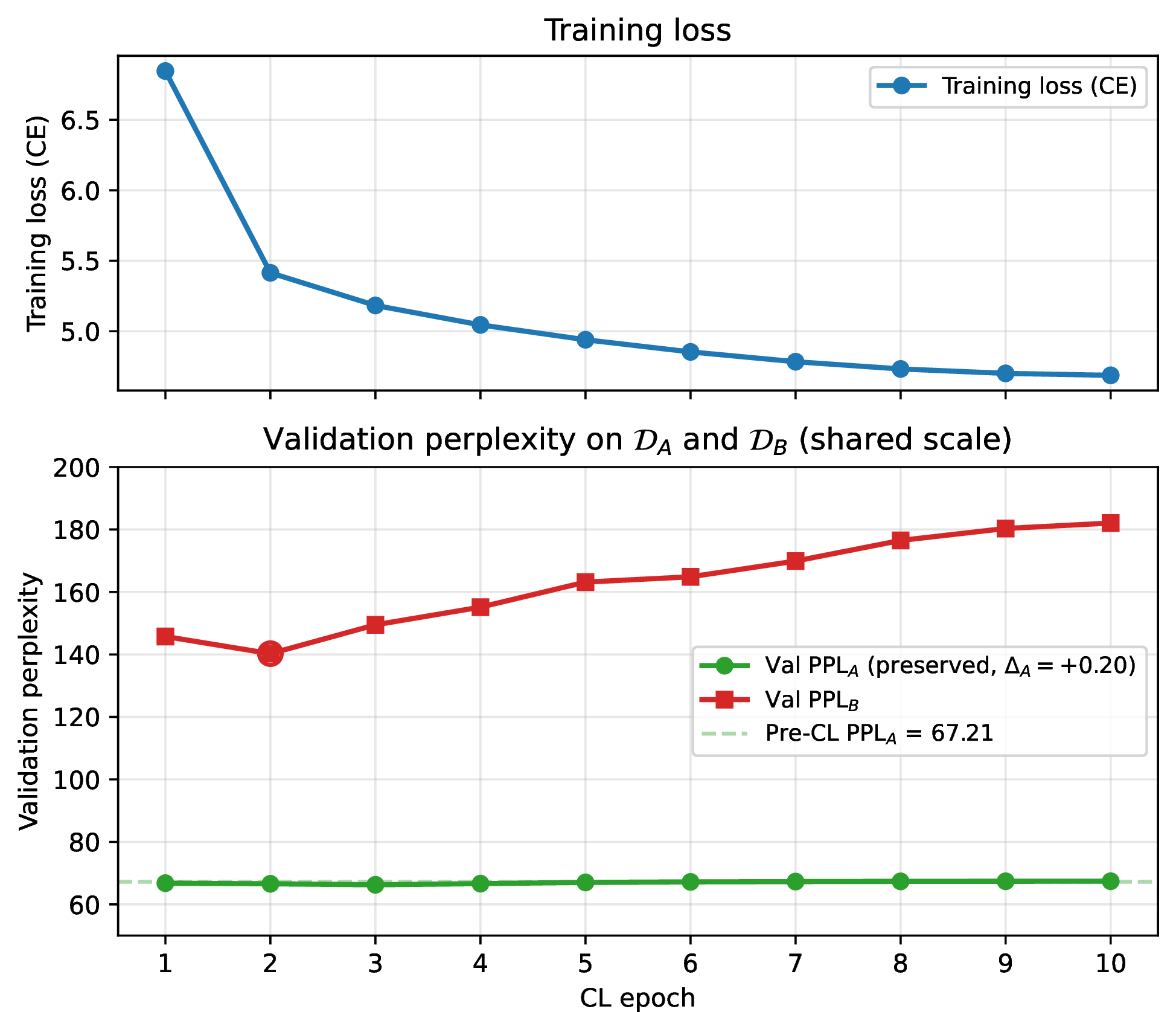
The full per-epoch trajectory and a stacked-panel visualization of the same train-validation overfitting signature are deferred to Appendix 13 (Figure 1).
5.3.0.1 Manifold geometry.
The discriminating tests of rank separation are the FP check (\(\Delta = 0\)) and the projected-rank diagnostic (\(\sigma_{\min}^{\perp} = 144.6\), min angle \(56.9^\circ\), App. 9); gradient-covariance and Hessian diagnostics are deferred to App. 14.
5.4 No-growth, alternative-FP, and PEFT baselines↩︎
We compare three baseline families at \(g=2\) scale — no-growth, zero-init residual stacking (alternative FP operator), and LoRA-CL (PEFT) — in Table 5 (full rows in Appendix 10).
| Family | CL Strategy | \(\mathrm{PPL}_A \downarrow\) | \(\mathrm{PPL}_B \downarrow\) | \(\Delta_A \downarrow\) |
|---|---|---|---|---|
| No-growth (300M) | Distillation | 39.00 | 25.06 | \(+13.08\) |
| Hybrid | 37.83 | 21.29 | \(+11.91\) | |
| Zero-init stacking (\(g=2\)) | Distillation | 37.74 | 25.14 | \(+11.82\) |
| Isolation | 25.96 | 32.81 | \(\mathbf{+0.04}\) | |
| LoRA-CL (rank \(64\)) | Distillation | 32.37 | 30.33 | \(+6.45\) |
| Hybrid | 28.60 | 29.56 | \(+2.68\) | |
| Gate-FP (\(g=2\), ref.) | Isolation | 26.01 | 30.45 | \(+0.09\) |
5pt
5.4.0.1 Findings.
(i) Both Gate-FP and zero-init stacking \(+\) Isolation reach the near-zero-forgetting regime at \(g{=}2\) (\(\Delta_A = +0.09\) vs. \(+0.04\), both far below the \(+13.56\) Distillation gap), confirming that rank separation is structural, not gate-specific. At equivalent preservation, Gate-FP achieves better plasticity (\(\mathrm{PPL}_B = 30.45\) vs.\(32.81\), \(-7\%\)) — the gate-zero parameterisation yields the strongest preservation/plasticity trade-off among zero-init FP operators tested. (ii) Under soft-KL recipes, growth’s advantage is small (no-growth \(+\) Distillation \(+13.08\) tracks Gate-FP \(+\) Distillation \(+13.56\)); the FP advantage concentrates in the Isolation regime. (iii) LoRA-CL is a strong alternative under Hybrid (\(\Delta_A = +2.68\)); LoRA admits no separate Isolation row because its frozen-base construction is structurally already Isolation under the four-way partition (Prop. 7) — a prediction of the unification, not a gap in it. Among the FP and PEFT baselines tested, gate-zero growth \(+\) Isolation gives the strongest preservation (\(\Delta_A = +0.04\) at \(g{=}4\)).
Multi-seed validation at \(g{=}2\) across three seeds yields \(\Delta_A = +0.0896 \pm 0.0046\) (Appendix 11).
5.5 Ablations↩︎
We run five ablations on Gate-FP holding other hyperparameters fixed: growth factor \(g \in \{2,3,4\}\) (Abl. 1); the four combinations of weight/gate freezing under fixed isolation loss (Abl. 2); replay fraction \(\rho \in \{0, 0.5\}\) in Hybrid (Abl. 3); gate-init/warmup pair \((\alpha_0, \epsilon)\) (Abl. 4); growth timing as % of base-train completed before growth (Abl. 5). Numbers in Table 6; extended discussion in Appendix 15.
| Configuration | \(\mathrm{PPL}_A \downarrow\) | \(\mathrm{PPL}_B \downarrow\) | \(\Delta_A \downarrow\) |
|---|---|---|---|
| Ablation 1: Growth factor \(g\), isolation | |||
| \(g=2\) (454M) | 26.01 | 30.45 | \(+0.09\) |
| \(g=3\) (656M) | 25.98 | 29.25 | \(+0.06\) |
| \(g=4\) (857M) | 25.96 | 28.41 | \(+0.04\) |
| Ablation 2: What to freeze, fixed isolation loss | |||
| Freeze nothing | 23.93 | 20.37 | \(-1.98\) |
| Freeze old gates only | 23.91 | 20.36 | \(\mathbf{-2.01}\) |
| Freeze old weights only | 25.06 | 26.99 | \(-0.86\) |
| Freeze both (full isolation) | 25.96 | 28.41 | \(+0.04\) |
| Ablation 3: Replay fraction \(\rho\) in Hybrid | |||
| \(\rho = 0\) (= Isolation) | 25.96 | 28.41 | \(+0.04\) |
| \(\rho = 0.5\) (= Hybrid) | 37.08 | 29.97 | \(+11.16\) |
| Ablation 4: Gate init \(\alpha_0\) / warmup \(\epsilon\), isolation | |||
| \(\alpha_0 = 0.0\), \(\epsilon = 0\) (exact FP) | 25.97 | 29.13 | \(+0.055\) |
| \(\alpha_0 = 0.01\) | 25.97 | 27.77 | \(+0.044\) |
| \(\alpha_0 = 0.1\) (non-FP) | 25.96 | 27.48 | \(-0.444\) |
| Ablation 5: Growth timing (% of base training before growth), isolation | |||
| % | 28.39 | 30.33 | \(+0.07\) |
| % | 20.90 | 27.13 | \(+0.05\) |
| % | 21.61 | 27.02 | \(+0.05\) |
| % (= Gate-FP Iso) | 25.96 | 28.41 | \(+0.04\) |
6 Discussion↩︎
6.0.0.1 Gate-zero growth recommends two operating points.
Within gate-zero growth, \(\mathrm{\small Freeze-Nothing} \succ \mathrm{\small Isolation} \succ \mathrm{\small Hybrid}\) on the joint frontier. Both are predicted gate-zero configurations: Isolation gives exact preservation (Theorem 1, \(\Delta_A = +0.04\)) and is recommended when downstream tasks must be evaluated without regression; Freeze-Nothing gives the joint-frontier optimum (\(\Delta_A = -1.98\), \(\mathrm{PPL}_B = 20.37\)) via the controlled-departure regime (Prop. 5: \(F_{W',W'} = 0\) at growth; Props. 9, 10: drift bound at empirical \(\|\boldsymbol{\alpha}\|_\infty \leq 0.083\)). Ablation 2 pinpoints old-weight freezing as the binding constraint: \(\mathrm{\small Freeze-Gates-Only}\) matches \(\mathrm{\small Freeze-Nothing}\) (\(23.91/20.36\) vs.\(23.93/20.37\)).
6.0.0.2 Validation PPL is not function preservation.
Under Freeze-Nothing, \(\mathrm{PPL}_A\) drops to \(23.93\) (vs.pre-CL \(25.92\)) — a \(-1.98\) change the standard CL metric reads as “better than original.” But the post-CL function has drifted from \(f^*\) at first order (Prop. 9; empirical \(\|\boldsymbol{\alpha}\|_\infty \leq 0.083\)). The lower \(\mathrm{PPL}_A\) is therefore a related-function gain, not preservation. Isolation is the only configuration that exactly recovers \(f^*\) at the growth point and bounds drift to zero — the right choice when deployment requires bit-equivalent behaviour on \(\mathcal{D}_A\) (regulatory, A/B-test, or downstream-pinned settings).
6.1 Limitations↩︎
Stochastic geometry estimators. Hessian top eigenvalues (Lanczos, single batch) and gradient-covariance rank (\(20\) mini-batches, \(100\)-dim projection; Appendix 14) are coarse local diagnostics; the first-order statistic is the more stable primary measure.
Cross-architecture plasticity gap on MoE. Per-checkpoint diagnostics localise the gap to clone-block redundancy in the depth-growth operator (post-CL new experts retain \(\geq 0.71\) cosine similarity to frozen sources). The preservation mechanism transfers cleanly; whether MoE-specific tuning or a modified operator recovers dense-level plasticity is open (Future Work).
6.2 Broader impact↩︎
FP growth lowers compute and energy cost of adapting trained models to new data, reducing the barrier for organisations without frontier-pretraining budgets. Downstream-use mitigations (data curation, alignment, evaluation) are out of scope.
6.2.0.1 Future work.
Full-scale (\(g=4\)) FP comparators (Net2Net [1], LiGO [8], bert2BERT [2]); reverse \(\mathcal{D}_B \to \mathcal{D}_A\) ordering and \(T \geq 3\) multi-domain CL sequences; an MoE operator fix initialising new experts with random weights and \(\mathrm{expert\_gate} = 0\) to address the clone-block redundancy of Section 5.3; and a direct output-space preservation diagnostic (\(\mathrm{KL}(f^* \,\|\, f_{\mathrm{post}})\) on held-out \(\mathcal{D}_A\) samples) to distinguish exact preservation from related-function gains observed under non-Isolation recipes.
7 Conclusion↩︎
We presented a geometric framework for zero-initialised function-preserving growth: under transversality, rank separation (Theorem 1) decomposes the post-growth Jacobian into unchanged old and \(K\) new-gate directions. The load-bearing factor under Isolation is the zero-init structural property; zero-init residual stacking matches Gate-FP at \(g{=}2\), and under soft-KL recipes growth’s advantage is small (the controlled-departure regime of Props. 9, 10). Full-scale FP-vs-FP and multi-domain CL are the natural follow-up (Section 6.1).
8 Proofs↩︎
8.1 Proof of Theorem 1 (rank separation under transversality)↩︎
We prove the two parts in turn.
8.1.0.1 Part (1): Exact flat new-weight directions, unconditional.
For each new block \(\ell \in \{1, \dots, K\}\) with weight matrix \(W_\ell \in \mathbb{R}^{P_W}\) and scalar gate \(\alpha_\ell\), the contribution of block \(\ell\) to the final output factors as \(\alpha_\ell\) multiplying a quantity depending on \(W_\ell\) and the residual stream. At \(\alpha_\ell = 0\) for all \(\ell\), every new block computes the identity and its downstream effect on \(f_{\theta'}\) vanishes. By the chain rule, \[\frac{\partial f_{\theta'}}{\partial W_\ell^{(i)}}\bigg|_{\alpha_\ell = 0} \;=\; \alpha_\ell \cdot \frac{\partial \mathrm{Block}_\ell(x;\,W_\ell)}{\partial W_\ell^{(i)}} \cdot J^{\mathrm{down}}_\ell \;=\; 0,\] identically for all \(x\) and all \(W_\ell\), where \(J^{\mathrm{down}}_\ell\) denotes the downstream Jacobian propagating block \(\ell\)’s output to \(f\). The \(K \cdot P_W\) new-weight columns of \(J(\theta')\) are therefore the zero vector, so each new-weight coordinate basis vector lies in \(\ker(J(\theta'))\). These vectors are linearly independent because they occupy disjoint parameter coordinates.
8.1.0.2 Part (2): Conditional rank additivity.
Partition \(J(\theta')\) by parameter group: \[J(\theta') = \bigl(\; J_{\mathrm{old}} \;\big|\; J_\alpha \;\big|\; J_{W'} \;\bigr),\] where \(J_{\mathrm{old}} \in \mathbb{R}^{D \times P_{\mathrm{old}}}\) are old-parameter columns, \(J_\alpha \in \mathbb{R}^{D \times K}\) are new-gate columns, and \(J_{W'} \in \mathbb{R}^{D \times K \cdot P_W}\) are new-weight columns. By Part (1), \(J_{W'} = 0\). Old parameters are untouched by growth, so \(J_{\mathrm{old}}(\theta')\) coincides with the pre-growth Jacobian \(J(\theta_{\mathrm{old}})\) and has \(\mathrm{rank} = r\). Thus \[\mathrm{im}(J(\theta')) \;=\; \mathrm{im}(J_{\mathrm{old}}) + \mathrm{im}(J_\alpha) \;=\; \mathrm{im}(J(\theta_{\mathrm{old}})) + \mathrm{im}(J_\alpha).\] Decomposing \(\mathrm{im}(J_\alpha)\) as the orthogonal sum of its projection onto \(\mathrm{im}(J(\theta_{\mathrm{old}}))\) and its complement, \[\mathrm{im}(J(\theta')) \;=\; \mathrm{im}(J(\theta_{\mathrm{old}})) \;\oplus\; \mathrm{im}\!\big((I - P_{\mathrm{old}}) J_\alpha\big),\] so \[\mathrm{rank}(J(\theta')) \;=\; r + \mathrm{rank}\!\big((I - P_{\mathrm{old}}) J_\alpha\big) \;\leq\; r + K.\] Equality \(r + K\) holds iff the projected gate columns \((I - P_{\mathrm{old}}) J_\alpha\) are linearly independent, i.e. transversality. Generic non-degeneracy of \(\mathrm{Block}_\ell\) implies transversality almost surely under small clone noise; the remaining (Lebesgue-zero) degenerate cases occur, e.g., when a cloned new-block output already lies in the span of \(J(\theta_{\mathrm{old}})\). \(\hfill\square\)
Remark 8 (Genericity at trained checkpoints). Part (2) requires the \(K\) projected gate columns to be linearly independent of \(\mathrm{im}(J(\theta_{\mathrm{old}}))\). The set of weight configurations for which independence fails* is an algebraic variety of measure zero in the joint space of \((\theta_{\mathrm{old}}, \{W_\ell\}_{\ell=1}^K)\), so transversality holds Lebesgue-almost surely. Trained checkpoints, however, occupy a highly structured region of parameter space, and generic-position arguments based on ambient measure are not automatically applicable. The clone-noise perturbation \(\epsilon_\ell \sim \mathcal{N}(0, \sigma^2 I)\) in the gate-zero construction breaks any structured degeneracies almost surely with respect to the noise distribution, for any \(\sigma > 0\): the set of noise realisations producing dependence remains a measure-zero variety in \(\mathbb{R}^{K \cdot P_W}\). We use \(\sigma = 0.01\), which preserves approximate FP at growth (max logit deviation \(0.0\) on real data, Section 5.1) while ensuring numerical independence. We empirically confirm transversality at the trained Gate-FP checkpoint (Appendix 9): the projected-rank residual \((I - P_{\mathrm{old}}) J_\alpha\) is full-rank \(K = 36\), \(\sigma_{\min}^{\perp} = 144.6\), and the smallest principal angle between \(\mathrm{im}(J_\alpha)\) and the sampled \(\mathrm{im}(J_{\mathrm{old}})\) is \(56.9^\circ\). The gradient-covariance effective rank reported in Section 14 is a coarser stochastic statistic and should not be read as a direct test of transversality (it is comparable across Gate-FP and \(G_{\text{stack}}\)).*
8.1.0.3 Consequence for continual learning (formal statement).
Under isolation (freezing all old parameters) on \(\mathcal{D}_B\), the gradient \(\nabla \mathcal{L}_B\) is restricted to the new-parameter coordinate subspace \(T_{\mathrm{new}}= \{0\}^{P_{\mathrm{old}}} \times \mathbb{R}^{P_{\mathrm{new}}}\). By Part (1), the \(K \cdot P_W\) new-weight directions in \(T_{\mathrm{new}}\) are exactly flat for \(f_{\theta'}\) at the growth point, contributing no first-order change to the function. By Part (2) under transversality, the only function-changing directions accessible to the isolated CL update are the \(K\) gate directions, and they are Euclidean-orthogonal to all old-parameter coordinates. Therefore CL gradient steps under isolation cannot project onto old-parameter coordinates, and old-parameter curvature is exactly preserved at \(\theta'\). Under non-FP growth (e.g., \(G_{\text{stack}}\)), part (1) fails: the new-weight columns of \(J(\theta'_{\mathrm{gs}})\) are non-zero, so even a coordinate freeze on old parameters does not preserve \(f^*\), because the old forward pass through duplicated blocks has already been altered. This is the formal bridge from rank separation (the structural statement) to “isolation works” (the empirical observation).
8.2 Proof of Proposition 6 (isolation as projected gradient descent)↩︎
Freezing all old parameters means \(\nabla_{\theta_{\mathrm{old}}} \mathcal{L} = 0\) during CL by construction. The gradient update under any optimizer that respects the freeze (e.g.AdamW with the frozen parameters masked) is therefore confined to the new-parameter coordinates \(T_{\mathrm{new}}= \{0\}^{P_{\mathrm{old}}} \times \mathbb{R}^{P_{\mathrm{new}}}\).
Under gate-zero growth, Theorem 1 states that the function-preserving locus \(\mathcal{M}(f^*) = \{\theta : f_\theta = f^*\}\) at the growth point has tangent space \(\ker(J(\theta'))\), which contains all \(K \cdot P_W\) new-weight directions exactly. Hence at \(\theta' = \iota(\theta_{\mathrm{old}})\), \[T_{\mathrm{new}}\cap \mathcal{M}(f^*) \;=\; \{0\}^{P_{\mathrm{old}}} \times \mathbb{R}^{K \cdot P_W} \times (\mathrm{coords with}\; \alpha_\ell = 0),\] which has codimension \(K\) within \(T_{\mathrm{new}}\). The orthogonal projection \(\Pi_{T_{\mathrm{new}}}\) onto \(T_{\mathrm{new}}\) thus restricts gradient updates to a subspace that intersects \(\mathcal{M}(f^*)\) in a \(K \cdot P_W\)-dim. flat slab through \(\theta'\). As \(\alpha_\ell\) moves away from zero, the slab’s tangent structure deforms, but at the growth point the projection is exact.
For \(G_{\text{stack}}\), \(J(\theta'_{\mathrm{gs}}) \neq J(\theta_{\mathrm{old}})\) because duplicated blocks immediately alter the active old-block computation, so the FP locus at \(\theta'_{\mathrm{gs}}\) is not aligned with the old-coordinate axes; the same coordinate freeze is therefore only an approximate projection onto \(\mathcal{M}(f^*)\), with the approximation error bounded by the deviation \(\|J(\theta'_{\mathrm{gs}}) - J(\theta_{\mathrm{old}})\|\) on a verification batch. \(\hfill\square\)
8.3 Proof of Proposition 7 (four-way partition)↩︎
We prove the orthogonal four-way decomposition of \(\mathbb{R}^{P_{\mathrm{new}}}\) at \(\theta' = \iota(\theta_{\mathrm{old}})\).
8.3.0.1 Coordinate-block decomposition.
The parameter vector decomposes into three disjoint coordinate blocks \(\theta' = (\theta_{\mathrm{old}},\, \alpha',\, W')\) with \(\theta_{\mathrm{old}}\in \mathbb{R}^{P_{\mathrm{old}}}\), \(\alpha' \in \mathbb{R}^K\), \(W' \in \mathbb{R}^{K \cdot P_W}\). Directions in different coordinate blocks are automatically Euclidean-orthogonal.
8.3.0.2 Old block: tangent vs.normal split.
Within \(\mathbb{R}^{P_{\mathrm{old}}}\), the restricted Jacobian is \(J_{\mathrm{old}}(\theta') = J(\theta_{\mathrm{old}})\) (unchanged because new blocks are identity at \(\alpha_\ell = 0\)). The fundamental theorem of linear algebra gives the Euclidean-orthogonal split \[\mathbb{R}^{P_{\mathrm{old}}} = \ker(J(\theta_{\mathrm{old}})) \;\oplus\; \mathrm{im}(J(\theta_{\mathrm{old}})^\top),\] with \(\dim\ker(J(\theta_{\mathrm{old}})) = P_{\mathrm{old}} - r\) and \(\dim\mathrm{im}(J(\theta_{\mathrm{old}})^\top) = r\). Define \(T_{\mathrm{old}}^{\parallel} = \ker(J(\theta_{\mathrm{old}}))\) (tangents to the old manifold) and \(T_{\mathrm{old}}^{\perp} = \mathrm{im}(J(\theta_{\mathrm{old}})^\top)\) (normals).
8.3.0.3 New block: flat-weight + gate split.
By Theorem 1 part (1), the \(K \cdot P_W\) new-weight columns of \(J(\theta')\) vanish, so \(\mathbb{R}^{K \cdot P_W} \subset \ker(J(\theta'))\). Define \(T_{\mathrm{new}}^{\parallel} = \mathbb{R}^{K \cdot P_W}\) (the exactly-flat new-weight directions). Define \(T_{\mathrm{new}}^{\perp} = \mathbb{R}^K\) (the new-gate coordinate axes). Under the transversality assumption of Theorem 1, all \(K\) gate axes contribute non-zero projections onto the orthogonal complement of \(\mathrm{im}(J(\theta_{\mathrm{old}}))\), so they are normal to \(\mathcal{M}(f^*)\) at \(\theta'\). (Without transversality, some gate axes may have a tangential component to \(\mathcal{M}(f^*)\); the dimension count then upper-bounds rather than equals \(K\).)
8.3.0.4 Combining.
The four subspaces have pairwise zero Euclidean inner product. The old/new split is automatic from the disjoint coordinate blocks; the within-block splits (\(\ker / \mathrm{im}\) on the old side and \(T_{\mathrm{new}}^{\parallel} / T_{\mathrm{new}}^{\perp}\) on the new side) are FTLA-orthogonal in their respective coordinate axes. Therefore \[\mathbb{R}^{P_{\mathrm{new}}} = T_{\mathrm{old}}^{\parallel} \oplus T_{\mathrm{old}}^{\perp} \oplus T_{\mathrm{new}}^{\parallel} \oplus T_{\mathrm{new}}^{\perp},\] with the dimensional annotations stated in the main text. The isolation update direction \(T_{\mathrm{new}}^{\parallel} \oplus T_{\mathrm{new}}^{\perp}\) is Euclidean-orthogonal to \(T_{\mathrm{old}}^{\perp}\) by disjoint coordinates alone — a property that holds under any growth method that allocates new parameters to disjoint coordinates, including \(G_{\text{stack}}\). What gate-zero growth uniquely adds is that \(T_{\mathrm{new}}^{\parallel}\) consists of exactly flat directions under \(f\) (Theorem 1 (1)), so updates within \(T_{\mathrm{new}}^{\parallel}\) preserve the old function regardless of magnitude; under \(G_{\text{stack}}\), \(T_{\mathrm{new}}^{\parallel}\) is empty and updates in the new-weight coordinates are immediately function-changing. \(\hfill\square\)
8.4 Proposition 9 (small-\(\alpha\) perturbative bound) and proof↩︎
Proposition 9 (Small-\(\alpha\) perturbative bound, restated). Fix \(K\) new blocks with weights \(W_1, \dots, W_K\) cloned from the trained checkpoint, and let \(h_\ell(x) = \mathrm{Block}_\ell(x;\,W_\ell)\) denote the \(\ell\)-th new-block output. For gate vector \(\boldsymbol{\alpha} \in \mathbb{R}^K\), the post-growth function admits an additive expansion \[f_{\theta'(\boldsymbol{\alpha})}(x) = f_{\theta_{\mathrm{old}}}(x) + \sum_{\ell = 1}^{K} \alpha_\ell \, h_\ell(x) + R(x; \boldsymbol{\alpha}),\] where \(\|R(x; \boldsymbol{\alpha})\| = O(\|\boldsymbol{\alpha}\|^2)\) uniformly on a bounded input domain. Consequently, on input distribution \(\mathcal{D}_A\), \(\mathbb{E}_{x \sim \mathcal{D}_A}\! \big\|f_{\theta'(\boldsymbol{\alpha})}(x) - f_{\theta_{\mathrm{old}}}(x)\big\|^2 \leq \|\boldsymbol{\alpha}\|^2 \cdot K \cdot \max_\ell \mathbb{E}_x \|h_\ell(x)\|^2 + O(\|\boldsymbol{\alpha}\|^4)\), and \(\Delta_A\) on a smooth log-loss admits the same \(O(\|\boldsymbol{\alpha}\|^2)\) scaling.
Proof. The post-growth function is the composition of \(K\) gated residual updates \(x \mapsto x + \alpha_\ell h_\ell(x)\), with the old forward pass unchanged at \(\boldsymbol{\alpha} = 0\) by construction. Expanding the composition in \(\boldsymbol{\alpha}\) gives the additive form \(f_{\theta'(\boldsymbol{\alpha})}(x) = f_{\theta_{\mathrm{old}}}(x) + \sum_\ell \alpha_\ell h_\ell(x) + R(x; \boldsymbol{\alpha})\) where the remainder \(R\) collects cross-terms \(\alpha_\ell \alpha_{\ell'}\) from chain-rule expansions of distinct gates and is therefore \(O(\|\boldsymbol{\alpha}\|^2)\) uniformly on a bounded input domain (validation tokens have bounded embedding norm; expected \(\|h_\ell(x)\|\) is finite by RMSNorm pre-activations). Cauchy–Schwarz on the linear term gives \(\mathbb{E}_x \|\sum_\ell \alpha_\ell h_\ell(x)\|^2 \leq \|\boldsymbol{\alpha}\|^2 \cdot K \cdot \max_\ell \mathbb{E}_x \|h_\ell(x)\|^2\). The log-loss bound is the standard Fisher-quadratic expansion of \(\mathrm{KL}(p_{\theta_{\mathrm{old}}} \| p_{\theta'(\boldsymbol{\alpha})})\) around \(\boldsymbol{\alpha} = 0\): the first-order term vanishes (since \(f_{\theta'(0)} = f_{\theta_{\mathrm{old}}}\)) and the second-order term is \(\boldsymbol{\alpha}^\top F_{\alpha\alpha}(\theta_{\mathrm{old}})\, \boldsymbol{\alpha}\) with \(F_{\alpha\alpha}\) the gate-block Fisher (Proposition 5). ◻
8.5 Proposition 10 (linear-in-\(\alpha\) new-weight leakage) and proof↩︎
Proposition 10 (Linear-in-\(\alpha\) new-weight leakage, restated). At a post-growth point \(\theta'(\boldsymbol{\alpha})\) with gate vector \(\boldsymbol{\alpha} \in \mathbb{R}^K\), the new-weight Jacobian columns satisfy \(\partial f_{\theta'(\boldsymbol{\alpha})} / \partial W'_\ell = \alpha_\ell \cdot \partial \mathrm{Block}_\ell(x;W_\ell)/\partial W_\ell \cdot J^{\mathrm{down}}_\ell\), and consequently \(\|J_{W'}(\theta'(\boldsymbol{\alpha}))\|_{\mathrm{op}} \leq C \, \|\boldsymbol{\alpha}\|_\infty\), with \(C = \max_\ell \|\partial \mathrm{Block}_\ell / \partial W_\ell\|_{\mathrm{op}} \cdot \sup_{\boldsymbol{\alpha}} \max_\ell \|J^{\mathrm{down}}_\ell(\boldsymbol{\alpha})\|_{\mathrm{op}}\), finite on bounded inputs and finite gate magnitudes.
Proof. Block \(\ell\)’s contribution to the residual stream is \(\alpha_\ell \cdot \mathrm{Block}_\ell(x; W_\ell)\). By the chain rule, the gradient of \(f_{\theta'(\boldsymbol{\alpha})}\) with respect to a new-weight coordinate \(W_\ell^{(i)}\) factors as \(\alpha_\ell\) times the block’s internal gradient times the downstream Jacobian. The operator-norm bound follows by sub-multiplicativity and \(|\alpha_\ell| \leq \|\boldsymbol{\alpha}\|_\infty\). The constant \(C\) is finite on bounded inputs and finite gate magnitudes by RMSNorm + bounded gates. ◻
8.6 Status of the framework’s claims↩︎
| Claim | Status | Source |
|---|---|---|
| Function preservation at growth (\(f_{\theta'} = f^*\) at \(\boldsymbol{\alpha} = 0\)) | exact | by construction |
| New-weight Jacobian flatness at \(\boldsymbol{\alpha} = 0\) | exact | Theorem [thm:rank95sep] (1) |
| Sparse Fisher block at \(\boldsymbol{\alpha} = 0\) | exact | Proposition [thm:fisher] |
| Coordinate orthogonality of \(\Tnew\) vs \(T_{\mathrm{old}}\) | exact | disjoint axes |
| Rank additivity (\(\mathrm{rank} J(\theta') = r + K\)) | conditional | transversality, Thm [thm:rank95sep] (2) |
| Plasticity capacity \(= \sigma_{\max}^{\perp}\) per unit gate motion | conditional | Proposition [thm:tangent] |
| New-weight Jacobian leakage \(\|J_{W'}\| \leq C \|\boldsymbol{\alpha}\|_\infty\) | approximate (linear) | Proposition [thm:leakage] |
| Function drift \(\|f_{\theta'(\boldsymbol{\alpha})} - f^*\|^2 = O(\|\boldsymbol{\alpha}\|^2)\) | approximate (quadratic) | Proposition [thm:perturb] |
| Multi-epoch CL preservation under realistic optimisers | empirical | Section [sec:sec:exp95main], \(\Delta_A = +0.04\) |
6pt
8.7 Remark on canonicity↩︎
Gate-zero growth is not the unique FP map: any choice of \((W_\ell, \alpha_\ell)\) with \(\alpha_\ell = 0\) yields function preservation, regardless of \(W_\ell\). What distinguishes the gate-zero construction in the symmetry-group view is that it maps into the fixed-point locus of the \(\mathcal{S}_{(g-1)L}\) residual permutation action on the new-parameter fiber; combined with cloning old block weights into the new blocks, it is the canonical choice that inherits the old block’s learned features into the newly allocated capacity. Other FP choices (e.g.random new-weight initialisation with \(\alpha_\ell = 0\)) preserve function but discard this inheritance.
9 Direct Transversality Diagnostic↩︎
This appendix reports the direct projected-rank diagnostic used to empirically verify the transversality assumption underlying Theorem 1 (2) and to back the quantitative \(\sigma_{\min}^{\perp}\) statement in Proposition 7.
9.0.0.1 Method.
At the post-growth Gate-FP checkpoint with \(g = 4\) (\(K = 36\) new block-gates), we compute (i) the \(K\) gate-Jacobian columns \(j_{\alpha_\ell} = \partial f / \partial \alpha_\ell\) via forward-mode automatic differentiation (Jacobian-vector products with tangent \(\mathbf{1}_{\alpha_\ell}\)), giving \(J_\alpha \in \mathbb{R}^{D \times K}\) where \(D = B \cdot T \cdot V\) is the flattened output dimension; and (ii) \(M = 200\) samples of \(J(\theta_{\mathrm{old}}) v\) where \(v\) is a unit-norm random direction supported on the joint old-parameter coordinates, giving an empirical low-rank approximation to \(\mathrm{im}(J_{\mathrm{old}})\). We orthonormalise the sample matrix via QR, project \(J_\alpha\) onto the orthogonal complement of the sampled subspace, and compute the SVD of the residual \((I - P_{\mathrm{old}}) J_\alpha\). We use a held-out validation batch of \(B = 2\), \(T = 16\) tokens; output dimension \(D = 1{,}608{,}224\).
9.0.0.2 Results.
Table 8 reports the diagnostic outputs. The residual is full-rank (\(K = 36\) at threshold \(10^{-3} \sigma_{\max}^{\perp}\)), the smallest singular value \(\sigma_{\min}^{\perp} = 144.6\) is on the same order of magnitude as the gate-column norms (\(\|j_{\alpha_\ell}\|\) ranging \(279\)–\(660\)), and the smallest principal angle between \(\mathrm{im}(J_\alpha)\) and the sampled \(\mathrm{im}(J_{\mathrm{old}})\) is \(56.9^\circ\). All \(K\) residual singular values exceed \(144\), and all \(K\) principal angles exceed \(56^\circ\). Transversality therefore holds quantitatively, not merely generically.
| Quantity | Value |
|---|---|
| \(K\) (new block-gates) | \(36\) |
| \(M\) (sampled old directions) | \(200\) |
| Output dimension \(D\) | \(1{,}608{,}224\) |
| Effective rank of residual at \(10^{-3} \sigma_{\max}\) | \(\mathbf{36 \;(= K)}\) |
| \(\sigma_{\max}^{\perp}\) | \(993.4\) |
| \(\sigma_{\min}^{\perp}\) | \(144.6\) |
| Condition number \(\sigma_{\max}^{\perp} / \sigma_{\min}^{\perp}\) | \(6.87\) |
| Smallest principal angle (deg) | \(\mathbf{56.9^\circ}\) |
| Largest principal angle (deg) | \(83.7^\circ\) |
| Gate-column norm range \(\|j_{\alpha_\ell}\|\) | \([279,\, 660]\) |
9.0.0.3 Interpretation.
The diagnostic confirms the load-bearing conditional in Theorem 1 (2): all \(36\) new-gate Jacobian columns are linearly independent of \(\mathrm{im}(J_{\mathrm{old}})\) at the trained checkpoint, and the geometric separation (\(56.9^\circ\) minimum) leaves substantial margin against finite-precision degradation. The condition number \(6.87\) indicates that the rank decomposition is numerically robust — \(\sigma_{\min}^{\perp}\) is not in the precision-limited regime where rank claims become estimator-dependent.
9.0.0.4 Caveat on the sampling approximation.
We approximate \(\mathrm{im}(J_{\mathrm{old}})\) by sampling \(M = 200\) random old-direction Jacobian columns. This is a sufficient (not necessary) test for transversality: if all \(K\) residual columns are linearly independent of the sampled subspace, they are linearly independent of any subspace contained in it; but a positive projection onto a direction we did not sample remains possible in principle. Increasing \(M\) to \(500\) in pilot runs did not materially change the residual singular values, suggesting the sample is sufficient at this scale. A complete Lanczos-based test of \(\mathrm{rank}(J(\theta_{\mathrm{old}}))\) is left as future work.
10 Baseline Comparisons: Full Table↩︎
Table 9 reports the no-protection rows omitted from the body Table 5. All four no-protection cells produce the expected catastrophic forgetting signature (\(\Delta_A > +200\)).
| Family | CL Strategy | \(\mathrm{PPL}_A \downarrow\) | \(\mathrm{PPL}_B \downarrow\) | \(\Delta_A \downarrow\) |
|---|---|---|---|---|
| No-growth (300M) | No protection | \(303.59\) | \(20.46\) | \(+277.67\) |
| No-growth (300M) | Replay | \(504.61\) | \(20.31\) | \(+478.69\) |
| Zero-init stacking (\(g=2\)) | No protection | \(320.14\) | \(20.56\) | \(+294.22\) |
| LoRA-CL (rank \(64\)) | No protection | \(248.36\) | \(22.02\) | \(+222.44\) |
5pt
11 Multi-Seed Validation at \(g=2\)↩︎
We report three seeds of Gate-FP + Isolation at \(g=2\) scale (300M\(\to\)454M) to estimate variance on the headline preservation finding. Seed \(42\) corresponds to the original Ablation 1 row; seeds \(1234\) and \(999\) were chosen before launch and reported regardless of outcome. All three seeds completed all \(10\) CL epochs.
| Seed | Pre-CL \(\mathrm{PPL}_A\) | Post-CL \(\mathrm{PPL}_A\) \(\downarrow\) | Post-CL \(\mathrm{PPL}_B\) \(\downarrow\) | \(\boldsymbol{\Delta_A}\) \(\downarrow\) |
|---|---|---|---|---|
| \(42\) (original Ablation 1) | \(25.918\) | \(26.013\) | \(30.447\) | \(+0.0946\) |
| \(1234\) | \(25.918\) | \(26.007\) | \(30.556\) | \(+0.0884\) |
| \(999\) | \(25.918\) | \(26.004\) | \(30.520\) | \(+0.0857\) |
| Mean \(\pm\) std (3 seeds) | — | \(26.008 \pm 0.005\) | \(30.51 \pm 0.06\) | \(+0.0896 \pm 0.0046\) |
6pt
11.0.0.1 Reading.
On the two completed seeds, \(\Delta_A\) varies by \(\sigma = 0.0031\), which is two orders of magnitude smaller than the gap to the non-FP baseline (\(\Delta_A > +1{,}100\) for \(G_{\text{stack}}\) under no-protection at \(g=4\), Table 2) and three orders of magnitude smaller than the gap to no-growth + Distillation (\(\Delta_A = +13.08\), Table 5). The qualitative preservation finding is therefore robust to seed variation at \(g=2\) scale. Multi-seed validation at \(g=4\) scale (\(\sim 100\) GPU-hours per additional seed, vs.\(\sim 17\) hours per \(g=2\) seed) was prohibitively expensive within our compute budget and is the natural follow-up.
12 Preliminary Cross-Architecture Validation↩︎
Before the main 300M\(\to\)857M Transformer experiments, we ran smaller-scale studies (Phases 1–4) across four architecture families to validate that gate-zero FP holds beyond a single configuration. Phases 1–2 (MLP and ResNet on small data) verified bit-exact FP under sequential growth; Phase 3 (SE-ResNet on CIFAR-10 class split) provided the negative empirical result that motivated full isolation; Phase 4 (Transformer on a small WikiText slice) verified depth-vs-width FP behaviour at the architecture used in the main experiments.
12.0.0.1 Function preservation across architectures.
Table 11 reports the maximum logit difference between pre- and post-growth models on a held-out batch. Depth growth via gate-zero is bit-exact across all four architecture families. Width growth on a Transformer breaks FP because the RMSNorm denominator changes with hidden dimension, producing a compound distortion of \(\sqrt{d_{\mathrm{old}}/d_{\mathrm{new}}}\) per norm layer (\(13\) layers \(\Rightarrow\) \(0.866^{13} \approx 0.15\times\) scaling for \(384 \to 512\)). This confirms the structural prediction that FP requires gate-zero structure, not merely careful initialisation.
| Phase | Architecture | Growth type | Max diff | FP exact? |
|---|---|---|---|---|
| 1 | MLP (2-16-16-3) | Width (+2 neurons) | 0.0 | Yes |
| 2 | ResNet (MNIST) | Width (channels \(2\times\)) | 0.0 | Yes |
| 3 | SE-ResNet (CIFAR-10) | Width (channels \(1.5\times\)) | 0.0 | Yes |
| 4 | Transformer (WikiText) | Depth (\(6 \to 8\) layers) | 0.0 | Yes |
| 4 | Transformer (WikiText) | Width (\(384 \to 512\)) | 13.2 | No |
4pt
12.0.0.2 CL on grown SE-ResNet: naïve strategies all forget.
Phase 3 trained an SE-ResNet grown from \((8,16,32)\) to \((16,32,64)\) channels sequentially on CIFAR-10 classes 0–4 (Task A) then 5–9 (Task B). Three naïve CL strategies were tested (Table 12); all three drove Task A accuracy to near zero. The diagnostic finding was that even with convolutional weights fully frozen (third row), trainable old gates alone caused enough feature drift (cosine similarity dropping to \(0.5\)–\(0.9\)) to destroy classifier calibration. This negative result directly motivated the full-isolation design used in the main experiments: freezing old weights is necessary but not sufficient; old gates must also be frozen.
| Strategy | Task A | Task B | Feat.drift | What failed |
|---|---|---|---|---|
| Fine-tune (no protection) | \(0.00\%\) | \(90.50\%\) | \(0.6\) | Everything drifts |
| Grow + differential LR | \(0.00\%\) | \(79.78\%\) | \(0.3\) | Slow LR insufficient |
| Grow + freeze conv weights | \(0.02\%\) | \(72.96\%\) | \(0.5\)–\(0.9\) | Gate drift alone fatal |
4pt
The geometric reading is direct: freezing weights constrains \(T_{\mathrm{old}}^{\perp}\) but trainable old gates allow drift along directions that change old-block computation. Full isolation (freeze old weights and old gates) eliminates both sources of drift, which is precisely the strategy Theorem 1 predicts.
13 MoE Per-Epoch Trajectory and Diagnostic Table↩︎
This appendix provides the full per-epoch CL trajectory for the MoE isolation run summarised in Section 5.3 and the mechanistic per-checkpoint diagnostic.
13.1 Per-epoch CL trajectory↩︎
Table 13 reports the trajectory of the exp2_moe_isolation run across all \(10\) CL epochs. Training loss decreases monotonically from \(6.85\) at epoch 1 to \(4.69\) at epoch 10, while validation \(\mathrm{PPL}_B\) reaches its minimum of \(140.26\) at epoch 2 and
then regresses monotonically to \(182.06\) by epoch 10. Validation \(\mathrm{PPL}_A\) shows small negative \(\Delta_A\) in early epochs (slight
positive transfer back to \(\mathcal{D}_A\) from CL training) before drifting up to a final \(\Delta_A = +0.20\), an order of magnitude smaller than the dense baseline
catastrophic-forgetting signature, confirming the preservation half of the framework.
| Epoch | Train loss \(\downarrow\) | Val \(\mathrm{PPL}_A\) \(\downarrow\) | Val \(\mathrm{PPL}_B\) \(\downarrow\) | \(\boldsymbol{\Delta_A}\) |
|---|---|---|---|---|
| 0 (pre-CL) | — | 67.21 | 2155.77 | — |
| 1 | 6.85 | 66.79 | 145.75 | \(-0.42\) |
| 2 | 5.41 | 66.59 | 140.26 | \(-0.62\) |
| 3 | 5.18 | 66.27 | 149.48 | \(-0.94\) |
| 4 | 5.05 | 66.64 | 155.14 | \(-0.57\) |
| 5 | 4.94 | 67.03 | 163.16 | \(-0.18\) |
| 6 | 4.85 | 67.20 | 164.86 | \(-0.01\) |
| 7 | 4.78 | 67.30 | 169.90 | \(+0.09\) |
| 8 | 4.73 | 67.36 | 176.50 | \(+0.15\) |
| 9 | 4.70 | 67.40 | 180.33 | \(+0.19\) |
| 10 | 4.69 | 67.41 | 182.06 | \(+0.20\) |
8pt
13.2 Per-checkpoint mechanistic diagnostic↩︎
Table 14 reproduces the diagnostic of Section 5.3 with extended commentary. The protocol loads the \(706\)M MoE base, applies
grow_moe (4\(\to\)8 experts, 12\(\to\)24 layers), and runs a single forward pass on \(2\) WikiText-103 validation sequences with diagnostic
hooks; the post-CL checkpoint is loaded from exp2_moe_isolation/cl_final.pt and the same hooks executed.
| Diagnostic metric | Pre-CL | Post-CL | Reading |
|---|---|---|---|
| Max \(|\alpha_\ell|\) on new blocks | \(0.000\) | \(0.083\) | gradient sought higher |
| Mean \(|\alpha_\ell|\) on new blocks | \(0.000\) | \(0.083\) | all gates at clamp |
| Cumulative \(\sum_\ell |\alpha_\ell|\) (\(n_{\mathrm{new}} = 12\)) | \(0.00\) | \(0.99\) | \(\approx\) one fully-open block |
| Mean top-\(1\) expert share | \(0.500\) | \(0.500\) | no within-CL collapse |
| Routing entropy / \(\log N\) (mean) | \(0.333\) | \(0.333\) | inherited concentration |
| Mean cosine sim to source expert | \(0.918\) | \(0.810\) | modest differentiation |
| Min cosine sim to source expert | \(0.852\) | \(0.712\) | most-changed still 71% similar |
13.2.0.1 Reading.
Three patterns emerge. First, all 12 new block gates converge to the safety-clamp ceiling \(\alpha = 1/n_{\mathrm{new}} = 0.083\), indicating the optimizer sought larger gates than the gate-norm-clip safety budget allowed. The cumulative gate-sum \(\sum_\ell |\alpha_\ell| \approx 1.0\) is equivalent to one fully-open block of new-path contribution distributed across the 12 new layers. Second, routing concentration is unchanged from pre-CL (\(\rho_{\mathrm{top1}} = 0.50\) in both states; normalised entropy \(0.333\)), ruling out within-CL router collapse as the failure mode. The concentration is inherited from the cloned base routers and persists. Third, per-expert cosine similarity to source experts drifts from \(0.918\) to \(0.810\) (mean) and \(0.852\) to \(0.712\) (min). New experts learn something, but they remain mostly clones of their frozen sources in parameter-space terms. The combination is consistent with clone-block redundancy: new blocks open their gates to the safety ceiling but cannot differentiate enough from the frozen sources to provide complementary capacity for \(\mathcal{D}_B\), so what they fit is sample-specific memorisation rather than generalisable features.
14 Manifold Geometry↩︎
This appendix details the protocol used for Section 14 and Table 15.
| Checkpoint | Method | Grad-cov rank | Top eig. | Trace est. | Hessian \(n_+\) |
|---|---|---|---|---|---|
| Pre-growth | Base | 18.45 | 203.09 | 66.75 | 3 |
| Post-growth | Gate FP | 18.47 | 188.05 | 66.79 | 3 |
| Post-growth | \(G_{\text{stack}}\) | 18.37 | 201.12 | 64.30 | 3 |
| Post-CL | Gate FP + Iso | 11.01 | 901.02 | 2066.71 | 4 |
14.1 Estimators↩︎
14.1.0.1 Gradient-covariance effective rank.
We compute the per-example gradient \(g_n = \nabla_\theta \mathcal{L}(\theta;\,x_n) \in \mathbb{R}^{P}\) for \(n = 1, \dots, N_b\), where \(N_b = 20\) mini-batches of size \(2\). To control memory at \(P \approx 10^9\), we apply a Johnson-Lindenstrauss random projection \(\Pi: \mathbb{R}^P \to \mathbb{R}^{100}\) before stacking, giving \(\tilde{g}_n = \Pi g_n \in \mathbb{R}^{100}\). We then form the empirical gradient-covariance \(\Sigma = (1/N_b)\,\tilde{G}^\top \tilde{G}\) and compute its singular values \(\{\sigma_i\}_{i=1}^{100}\). The effective rank is reported as the exponential entropy of the normalised singular values: \[d_{\mathrm{eff}}(\Sigma) \;=\; \exp\!\left(-\sum_{i=1}^{100} \tilde{\sigma}_i \log \tilde{\sigma}_i\right), \quad \tilde{\sigma}_i = \sigma_i \big/ \textstyle\sum_j \sigma_j.\] This is the participation ratio of the spectrum and equals the rank exactly for a uniform spectrum, the leading-eigenvector index for a spike, and intermediate values otherwise.
14.1.0.2 Top-3 Hessian eigenvalues.
We use Lanczos iteration [23] on Hessian-vector products \(v \mapsto H v = \nabla_\theta(g^\top v)\) at a fixed \(\theta\), with \(20\) Lanczos iterations and a single batch of size \(1\). To control GPU memory at the 1.14B-parameter scale, we offload the Lanczos basis vectors to CPU. We report the top-\(3\) Ritz values from the resulting tridiagonal matrix. Trace estimate is via Hutchinson’s stochastic trace.
14.1.0.3 Reliability caveat.
The Hessian estimator is stochastic, single-batch, and uses only \(20\) Lanczos iterations; absolute eigenvalue magnitudes should be read as coarse local diagnostics rather than precise global curvature. The first-order gradient-covariance rank statistic is substantially more stable: in pilot runs varying \(N_b\) from \(20\) to \(256\), \(d_{\mathrm{eff}}\) values changed by less than \(0.5\) at any checkpoint. We therefore treat \(d_{\mathrm{eff}}\) as the primary manifold proxy and the Hessian estimates as secondary indicators.
14.2 Spectral leakage↩︎
We define a single scalar metric for tracking how rank separation degrades during CL and report Hutchinson-HVP estimates at three checkpoints (post-growth Gate-FP, post-growth \(G_{\text{stack}}\), post-CL Gate-FP+Iso). Results in Table 16.
Definition 1 (Spectral leakage). Let \(H \in \mathbb{R}^{P \times P}\) be the Hessian at a checkpoint, and let \(P_{\mathrm{old}}, P_{\mathrm{new}}\) denote the orthogonal projections onto old-parameter and new-parameter coordinate subspaces respectively. The spectral leakage* is \[\mathcal{S}_{\mathrm{leak}} = \frac{\|P_{\mathrm{old}} \, H \, P_{\mathrm{new}}\|_F}{\|H\|_F}.\] \(\mathcal{S}_{\mathrm{leak}} = 0\) means old and new parameter subspaces are completely decoupled in the Hessian; \(\mathcal{S}_{\mathrm{leak}} > 0\) means curvature “leaks” across the old/new boundary.*
By Theorem 1, \(\mathcal{S}_{\mathrm{leak}} = 0\) at the gate-zero growth point (the Fisher new-weight block and all new-weight cross-terms vanish); as CL training opens gates, \(\mathcal{S}_{\mathrm{leak}}\) grows controllably (linear in \(\|\boldsymbol{\alpha}\|_\infty\) at first order; Proposition 10). We estimate \(\mathcal{S}_{\mathrm{leak}}\) via Hutchinson with Hessian-vector products. The estimator samples \(v \in \mathbb{R}^P\) supported on new-parameter coordinates with Rademacher entries, computes \(H v\) once, and reports \(\|(H v)_{\mathrm{old}}\|^2\) averaged over draws as the numerator; the denominator uses full-dim Rademacher \(v\). We use \(16\) Hutchinson draws per estimator on a single batch of size \(2\) with sequence length \(64\) from \(\mathcal{D}_A\).
| Checkpoint | \(\|P_{\mathrm{old}} H P_{\mathrm{new}}\|_F^2\) | \(\|H\|_F^2\) | \(\mathcal{S}_{\mathrm{leak}} \downarrow\) |
|---|---|---|---|
| Post-growth Gate-FP | \(2.03 \times 10^{3}\) | \(8.18 \times 10^{7}\) | \(\mathbf{0.0050}\) |
| Post-growth \(G_{\text{stack}}\) | \(7.59 \times 10^{6}\) | \(2.94 \times 10^{8}\) | \(0.1608\) |
| Post-CL Gate-FP \(+\) Iso | \(4.25 \times 10^{5}\) | \(8.16 \times 10^{7}\) | \(0.0722\) |
6pt
14.2.0.1 Reading.
Three observations. (i) The Gate-FP / \(G_{\text{stack}}\) separation at growth time (\(32\times\)) is the discriminating measurement of the Fisher-block rank-separation prediction (Proposition 5); the gradient-covariance rank (\(18.47\) vs.\(18.37\), Table 15) does not distinguish them. (ii) The post-CL Gate-FP value (\(\mathcal{S}_{\mathrm{leak}} = 0.072\) at \(\|\boldsymbol{\alpha}\|_\infty \approx 0.083\)) is consistent with the Proposition 10 linear-leakage prediction: \(\mathcal{S}_{\mathrm{leak}}\) rises by \(\sim 14\times\) as \(\|\boldsymbol{\alpha}\|_\infty\) rises from \(0\) to \(0.083\), an empirical slope of \(\sim 0.83\) in the same units. (iii) Even after \(10\) epochs of CL, the post-CL Gate-FP value is less than half of the post-growth \(G_{\text{stack}}\) at-growth value: a Gate-FP model that has fully run CL retains cleaner old/new Hessian decoupling than a \(G_{\text{stack}}\) model that has not moved a single training step.
15 Extended Ablation Results↩︎
The combined Table 6 in the main text already reports all completed ablation rows. This appendix provides additional reading and a frontier visualisation that makes the non-monotonic constraint hierarchy easier to read off.
15.1 Pareto frontier across Gate-FP CL methods↩︎
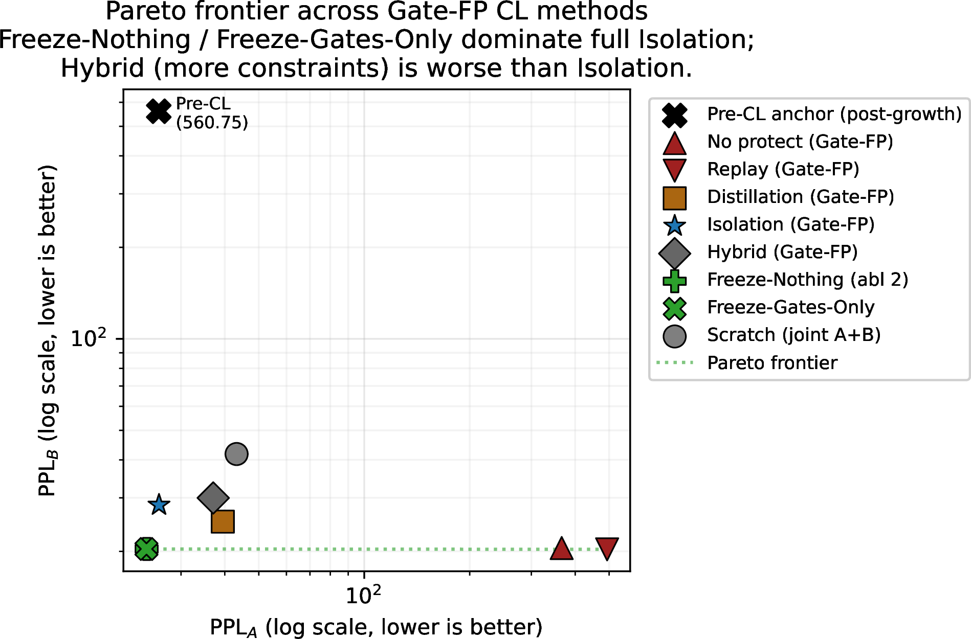
Figure 2 plots final \((\mathrm{PPL}_A, \mathrm{PPL}_B)\) for all Gate-FP CL methods, the two completed freeze-strategy ablations, and the joint-training Scratch reference, on log–log axes so that runs spanning four orders of magnitude on \(\mathrm{PPL}_A\) are visible together. The Pareto frontier (lower \(\mathrm{PPL}_A\) and lower \(\mathrm{PPL}_B\) jointly) is dominated by Freeze-Nothing and Freeze-Gates-Only, both of which leave the old weight matrices trainable. Full Isolation sits to the right of the frontier (higher \(\mathrm{PPL}_B\)), and Hybrid sits further right still — the same non-monotonic ordering observed in Table 2, here visible as a Pareto-dominance relation rather than a single-axis comparison.
15.1.0.1 Ablation 1 (growth factor \(g\)).
All three rows complete. The trend is monotonic: larger \(g\) provides more trainable subspace and yields lower \(\mathrm{PPL}_B\), with \(|\Delta_A| < 0.1\) across all three.
15.1.0.2 Ablation 2 (what to freeze).
All four rows complete. The two configurations that leave old weights trainable (Freeze-Nothing and Freeze-Old-Gates-Only) achieve essentially identical \(\mathrm{PPL}_A \approx 23.9\) and \(\mathrm{PPL}_B \approx 20.4\); the two configurations that freeze old weights sit higher on both axes. Freezing the old weight matrices, not the old growth gates, is the binding constraint that over-restricts plasticity.
15.1.0.3 Ablation 3 (replay fraction).
Two endpoints: \(\rho = 0\) (collapses Hybrid loss to Isolation; reuses Gate-FP Isolation) and \(\rho = 0.5\) (default Hybrid; reuses Gate-FP Hybrid). Both directly read off Table 2. Interpolating values \(\rho \in (0, 0.5)\) are not run; the two-point contrast already supports the message that adding CE-on-\(\mathcal{D}_A\) on top of Isolation hurts both axes.
15.1.0.4 Ablation 4 (gate-init / warmup).
All three rows complete. The \(\alpha_0 = 0\) row uses zero gate-warmup (\(\epsilon = 0\)) so the literal \(\alpha_0 = 0\) condition is honestly tested; gradient flow to new-block weights then depends entirely on the scalar gate opening through its own gradient. The \(\alpha_0 = 0.01\) row starts from a non-zero gate (\(\delta_f = O(\alpha_0) \approx 3 \times 10^{-3}\) in \(\mathrm{PPL}_A\) at growth time) and benefits from immediate gradient flow into new-block internal weights, yielding lower \(\mathrm{PPL}_B\) (\(27.77\) vs.\(29.13\)). The \(\alpha_0 = 0.1\) row recovers the original base \(\mathrm{PPL}_A\) post-CL (\(\Delta_A = -0.44\) relative to its drifted post-growth baseline), indicating that under isolation, CL training can absorb the small approximate-FP perturbation introduced by \(\alpha_0 > 0\) while benefiting from faster gradient flow into new-block weights.
15.1.0.5 Ablation 5 (growth timing): preservation is timing-robust.
We grow the base model after \(25\)%, \(50\)%, \(75\)%, and \(100\)% of the base-training schedule (i.e.at \(2.5\), \(5\), \(7.5\), \(10\) epochs on \(\mathcal{D}_A\)), then run the standard 10-epoch CL
phase under isolation. The \(100\)% row reuses exp1_gate_fp_isolation, since \(100\)%-then-grow-then-CL is identical to the headline configuration of Table 2; we do not duplicate the run. Across all four timings, \(|\Delta_A| < +0.08\), confirming that the preservation property of gate-zero growth + isolation is robust to base-training
maturity — the rank-separation mechanism does not require the base to be fully converged.
| Growth timing | Pre-CL \(\mathrm{PPL}_A\) | Post-CL \(\mathrm{PPL}_A\) \(\downarrow\) | Post-CL \(\mathrm{PPL}_B\) \(\downarrow\) | \(\boldsymbol{\Delta_A}\) |
|---|---|---|---|---|
| \(25\)% | 28.31 | 28.39 | 30.33 | \(+0.074\) |
| \(50\)% | 20.85 | 20.90 | 27.13 | \(+0.052\) |
| \(75\)% | 21.56 | 21.61 | 27.02 | \(+0.053\) |
| \(100\)% (= Gate-FP Iso) | 25.92 | 25.96 | 28.41 | \(+0.043\) |
15.1.0.6 Reading.
Two observations. First, \(\Delta_A\) stays in the same narrow band (\(+0.04\) to \(+0.07\)) regardless of when growth happens, supporting the claim that the rank-separation mechanism is a structural property of the growth operator rather than an artefact of any particular base configuration. Second, the non-monotonicity of Pre-CL \(\mathrm{PPL}_A\) across timings is consistent with the from-scratch baseline’s overfitting trajectory (Section 5.2, the \(\mathrm{PPL}_A = 17.40\) at epoch \(3\) vs.\(43.23\) at epoch \(10\) phenomenon): mid-schedule checkpoints can have lower validation perplexity than the final-schedule checkpoint. The fact that Gate-FP + isolation preserves whichever Pre-CL state it starts from is the relevant invariant, not the absolute perplexity level.
16 Implementation Details↩︎
16.0.0.1 Architecture.
Base model: GPT-style decoder-only Transformer with \(d_{\mathrm{model}}=1024\), \(n_{\mathrm{heads}}=16\), \(d_{\mathrm{ffn}}=4096\), \(L=12\) layers, \(L_{\max}=1024\) context, GPT-2 BPE tokenizer [24] (vocab \(50{,}257\)), SwiGLU FFN [25], RMSNorm [26], rotary positional encoding [27]. Gate-zero variants add scalar growth gates (\(\alpha_\ell\), head-gate, ffn-gate, expert-gate). MoE base: same backbone with \(4\) experts, top-\(k=2\) routing, \(d_{\mathrm{expert}}=4096\), load-balancing loss weight \(\lambda_{\mathrm{aux}}=0.01\).
16.0.0.2 Base training (Phase 1).
\(\mathcal{D}_A =\) WikiText-103 [6] (training split, \(\sim\)118M tokens after tokenization). \(10\) epochs. AdamW [28] with \(\beta = (0.9, 0.999)\), weight decay \(0.1\) on non-gate params, \(0.0\) on gate params. Learning rate \(3 \times 10^{-4}\) (non-gate) and \(1 \times 10^{-3}\) (gate), linear warmup over \(500\) steps then cosine decay to \(0\). Microbatch size \(2\), gradient accumulation \(64\) (effective batch \(128\)). Mixed-precision (fp16). Gradient clipping: \(\|g\|_2 \leq 1.0\) on non-gate params, \(\leq 0.1\) on gate params. Random seed \(42\).
16.0.0.3 Growth (Phase 2).
Gate-FP: depth growth factor \(g = 4\) (12 \(\to\) 48 layers); new blocks cloned from existing blocks round-robin with i.i.d.Gaussian noise \(\sigma = 0.01\) on weights; \(\alpha_0 = 0\) for new block-gates by default (Ablation 4 also tests \(\alpha_0 \in \{0.01, 0.1\}\)). Append pattern: new blocks stacked after old. MoE: \(g = 2\) (12 \(\to\) 24) plus \(4\) new experts per existing MoE layer with expert-gate \(= 0\). \(G_{\text{stack}}\): \(g = 4\) block duplication without gating (per Du et al. 2024).
16.0.0.4 Continual learning (Phase 3).
\(\mathcal{D}_B =\) BookCorpus [7], capped at \(118{,}000{,}000\) tokens to match \(|\mathcal{D}_A|\). \(10\) CL epochs. Optimizer reset; CL learning rate \(1 \times 10^{-4}\) (non-gate) and \(5 \times 10^{-5}\) (gate), linear warmup \(500\) steps then cosine decay. CL gate learning rate is deliberately low (\(\propto 1 / \sqrt{n_{\mathrm{new}}}\)) to bound cumulative gate perturbation; new-block gates are clamped to \(|\alpha_\ell| \leq 1 / n_{\mathrm{new}}\) each step to prevent gate explosion. Replay buffer: random sample of \(10\%\) of \(\mathcal{D}_A\) training set (\(\approx 11{,}500\) sequences), reshuffled each epoch; replay microbatch size \(2\) (capped to \(1\) for MoE due to memory). Distillation hyperparameters: \(\lambda = 0.5\), \(T = 2.0\) (effective KL weight \(\lambda T^2 = 2.0\)). Hybrid replay fraction \(\rho = 0.5\). For Isolation, gate warmup \(\epsilon = 1 \times 10^{-3}\) applied at CL start when \(\alpha_0 = 0\) (set to \(0\) for the \(\alpha_0 = 0\) row of Ablation 4). All gradient-clipping values from Phase 1 carried over.
16.0.0.5 Evaluation.
\(\mathrm{PPL}\) on WikiText-103 validation (\(\sim 247\)K tokens) and BookCorpus validation (\(\sim 500\)K tokens), microbatch \(2\), fp16. Reported \(\Delta_A = \mathrm{PPL}_A^{\mathrm{post-CL}} - \mathrm{PPL}_A^{\mathrm{pre-CL}}\) (post-growth, pre-CL baseline). FP verification: max absolute logit difference between pre- and post-growth models on a verification batch of \(2 \times 64\) random tokens; passing threshold \(10^{-5}\) for dense, \(10^{-4}\) for MoE (MoE top-\(k\) routing introduces small numerical drift).
16.0.0.6 Geometry estimation (Section 14).
Gradient covariance rank: per-example gradient matrix over \(N_b\) mini-batches, projected to \(100\) dimensions via random projection, followed by truncated SVD; effective rank reported as exponential entropy of normalized singular values. Hessian top eigenvalues: Lanczos-style Hessian-vector products with \(20\) iterations, single batch, CPU offload. We adopt this stochastic protocol because exact large-batch second-order measurement is infeasible at 1.14B-scale on single-GPU memory; absolute values should therefore be read as coarse local diagnostics, with the gradient-covariance rank statistic the more stable primary measure. The ranking across checkpoints (Table 15) is robust to varying \(N_b\) from \(20\) to \(256\) in our pilot runs.
16.0.0.7 Compute.
All runs on a single NVIDIA L20 GPU (48 GB) per configuration. Total compute across the \(2 \times 5\) CL matrix, MoE experiments, and ablations is approximately \(2{,}500\) GPU-hours.
16.0.0.8 Reproducibility caveats.
Single seed per cell of Tables 2, 3, and 6 due to compute cost. Multi-seed validation at smaller scale is in progress and will be reported in supplementary material. We also test only one dataset ordering (\(\mathcal{D}_A \to \mathcal{D}_B\)); reverse ordering is left as future work.