CASP: Learning-Augmented Offline Approximation with Verifiable Certificates and Bounded-Loss PAC Guarantees
July 16, 2026
Abstract
Machine-learned predictions can speed up offline NP-hard optimization, but asking a predictor what to do amounts to asking it to solve the problem, and committing an unchecked prediction forfeits every worst-case guarantee. CASP (Certificate-Augmented Solution Pruning) instead asks which parts of the search space may be ignored, and accepts each answer only after a sound polynomial-time verifier has checked it, so correctness never depends on prediction quality. We develop the learning theory of this design. The verifier makes the induced loss class uniformly bounded, so certificate parameters are learnable from \(\tilde{O}(\varepsilon^{-2}\log K)\) samples (\(K\) the maximum instance size), whereas the unverified commitment class admits no distribution-free rate and, under cost spread \(R\), none below \(\Omega(R/\varepsilon^2)\). Filtering noisy predictions by verifiable confidence dominates the standard min-combiner, with a margin we compute in closed form, and the prediction stays useful even given the LP, because it breaks ties on degenerate optimal faces, where every symmetric LP policy, meaning one whose commitments depend on the instance only through the verifiable confidence values, provably stalls. Experiments on five problems test the theory’s quantitative predictions. With trained predictors, unverified pruning loses up to \(26\%\) of the optimum under distribution shift, while the verified deployment of the same predictions loses nothing.
algorithms with predictions; learning-augmented algorithms; PAC learning; sample complexity; certificate verification; confidence filtering; LP degeneracy; offline approximation
1 Introduction↩︎
1.1 Motivation↩︎
Approximation algorithms face a bottleneck that has resisted progress for over a decade. For a large class of NP-hard problems the gap between the best inapproximability bound and the best known ratio has not moved: the \(\ln n\) factor for Set Cover is tight under \(\mathrm{P}\neq\mathrm{NP}\) [1], [2], and Vertex Cover cannot be approximated below \(2\) under the Unique Games Conjecture [3]. Learning-augmented algorithms offer a way around worst-case analysis: consult a machine-learned prediction at run time, beat the classical bound when the prediction is accurate, and fall back to it when it is not [4]–[7]. The successes, however, are almost entirely about online problems such as caching and scheduling, where the prediction concerns a future the algorithm cannot see. Only recently have a few works injected predictions into offline approximation [8]–[10], and they share one template: predict part of the optimal solution and prove that the ratio degrades gracefully with prediction error.
We believe progress has been slow because the online template hides a circularity when transplanted offline. Asking the predictor what to do on an NP-hard instance is self-defeating: a predictor strong enough to output a near-optimal solution has implicitly solved the problem, while a weaker predictor produces advice that no polynomial procedure can make trustworthy. Offline approximation is caught between a predictor too strong to exist and one too weak to use. The “ratio degrades with error” template softens the second horn but leaves the first untouched: the predictor still points at the solution. This paper asks whether predictions can be used so that the predictor answers a question strictly easier than the original problem, so that correctness survives arbitrarily wrong predictions, and so that good predictions can make exact solving polynomial.
1.2 Our approach↩︎
Our answer inverts the information flow. Instead of asking the predictor what to do, a positive signal, we ask what may be safely ignored, a negative signal, and we require the answer as a polynomial-time-verifiable certificate. A certificate asserts that a region of the search space can be removed; a verifier checks the assertion; only certificates that pass are used. This dissolves the circularity in three steps. First, deciding that a region need not be examined is typically far easier than finding the optimum, so the predictor answers a genuinely simpler question. Second, removing a region may keep some optimum intact, which we call OPT-preserving, or may inflate the optimum by at most a factor \(\rho\), which we call \(\rho\)-approximation-safe; this graded notion states exactly when the framework is exact and when it is approximate. Third, every certificate must pass the verifier, so a wrong prediction is at worst rejected and never causes an incorrect pruning; whenever \(\rho\,\alpha_{\mathrm{red}}\le\alpha\), in particular under OPT-preserving certificates with an exact reduced solve, the framework is never worse than its classical fallback (Theorem 3), in contrast to positive-signal methods whose guarantees lean on the prediction being good.
1.3 Contributions↩︎
Beyond formalizing CASP, our contributions concern learning, and they share one thesis, that checking, not the sign of the signal, is the resource.
The framework. A certificate system \((\mathcal{L},V,P)\) with two graded safety classes and five core results: pruning monotonicity, an OPT-preservation identity, composability, a robustness upper bound, and an exact-solvability condition (Section 3). Table 1 records, for every certificate in the paper, whether the verifier checks the safety level itself or only the underlying assertion.
A quantitative theory of confidence filtering. Filtering noisy predictions by a verifiable confidence signal dominates the standard min-combiner, and on an explicit Vertex Cover family we compute the asymptotic margin exactly: \(\min\{\eta[(C-\eta)+\beta(1-\eta)^2],\,\beta\}/(1+2\beta)\), zero at zero noise, increasing at small noise, and capped at the fallback gap (Theorem 16). The prediction is not redundant given the LP. On degenerate optimal faces every symmetric LP-commit policy (Definition 8) provably stalls, and the filter wins by a constant margin at every noise level because the prediction supplies the tie-break that no function of the LP confidences can (Theorem 17). Proposition 3 delimits when filtering cannot help, and a two-threshold filter recovers the high-noise regime at no extra sample cost (Proposition 4). Both quantitative results are equality instances of general theorems for decomposable families (Theorems 18 and 19), so the explicit families carry only the arithmetic.
Bounded loss, and its exact boundary. The verifier makes the loss class uniformly bounded, so certificate parameters are learnable with \(\tilde{O}(\varepsilon^{-2}\log K)\) samples, for single- and multi-parameter classes (Section 5); the structurally identical bare-commitment class has the same pseudo-dimension yet admits no distribution-free rate (Theorem 21, Lemma 4), and under bounded cost spread \(R\) its sample complexity is \(\Omega(R/\varepsilon^2)\) while CASP’s stays \(R\)-independent (Theorem 22). Certified optimality behaves the same way. CASP emits checkable proofs of exactness on a recognizable class (Theorem 20), the bare interface emits none, and a fair min-combiner adversary matches both guarantees (Section 7.4). These contrasts are properties of the prediction interface rather than complexity separations.
Instantiations. Five structurally diverse problems, with classical reductions recast as verifiable certificates: Set Cover, Vertex Cover with triggerable exact solvability on a named class and a planted distribution, Facility Location with a facility-integral exactness trigger, 0/1 Knapsack via reduced-cost fixing, and Steiner Tree via classical reduction tests (Sections 4.1–4.5). None of the individual reductions is new; the uniform certificate semantics laid over them is.
Experiments. Fourteen experiment groups test the theory’s quantitative predictions, from Monte-Carlo recomputation of the closed forms (E14) to trained predictors under distribution shift, where unverified pruning loses up to \(26\%\) of the optimum and the verified deployment of the same predictions loses nothing (E13).
2 Related Work↩︎
2.0.0.1 Algorithms with predictions.
The field began with online problems: competitive caching with learned advice [4], ski rental and scheduling [5], the survey of [6], prediction portfolios [7], a primal–dual treatment [11], and tight consistency–robustness trade-offs [12]. There the prediction concerns an unseen future, so consuming it uncritically is unavoidable. Offline the situation is different, and the recent offline line is the closest to this paper. [8] give prediction-augmented algorithms for minimum-weight feasible-subset problems in which the predictor supplies solution membership and the ratio degrades smoothly with prediction error; [9] study an \(\varepsilon\)-accurate prediction model; [10] break approximation barriers under edge predictions; [13] treat permutation problems. All of these commit a (partial) predicted solution and bound the damage as a function of prediction error. CASP differs on two axes. Correctness and the worst-case ratio are decoupled from prediction quality entirely, because nothing unverified is ever committed (Theorems 3 and 5); and the certificate interface supports guarantees that the commitment interface does not express, although a fair adversary with a fallback can match them, a boundary we prove rather than blur (Section 7.4). The algorithm of [8] serves as our positive-signal baseline in E10/E10\('\).
2.0.0.2 Learning for combinatorial solvers.
Closest in mechanism is machine-learned problem reduction, which trains a model to predict which variables can be deleted: graph reduction for maximum-weight clique [14], search-space classification for subset problems [15], and learned duals that warm-start exact algorithms [16]. These are negative signals in our sense, committed without a verifier, so an erroneous prediction silently destroys optimality; E13 quantifies the difference by deploying the same trained predictions with and without our verifier under distribution shift. In continuous optimization, safe screening rules [17], [18] delete variables of sparse learning programs through duality-based, per-variable, individually verifiable tests, which is the negative-signal-plus-soundness discipline of CASP with analytic rather than learned proposals. Data-driven algorithm configuration [19]–[23] supplies the pseudo-dimension machinery behind Section 5, but tuned parameters carry no per-instance guarantee; E5 compares against a configuration-style baseline without a verifier. Learning inside MILP solvers, to branch, to cut, to dive on predicted partial assignments [24], or to presolve [25], [26] (see [27] for a survey), and warm starts with predictions [28], accelerate search without shrinking the instance, whereas verified pruning shrinks the instance itself. The volume of [29] frames the broader beyond-worst-case agenda to which this work belongs.
2.0.0.3 Certifying algorithms and classical reductions.
A certifying algorithm returns, with each output, an easily checked witness of correctness [30]. CASP applies that discipline to predictions rather than to a fixed computation: an ML output is used only after a sound verifier accepts it, and on the class \(\mathcal{K}_{\log}\) the pipeline additionally emits a checkable proof of exact optimality (Theorem 20). The certificates themselves are classical. We reuse greedy and frequency bounds for Set Cover [1], [2], [31], [32], LP rounding and filtering for Facility Location [33]–[36] together with the long-documented LP tightness of its benchmarks [37], Nemhauser–Trotter persistency and the \(2k\) kernel for Vertex Cover [3], [38], [39], reduced-cost fixing for Knapsack [40]–[42], Steiner reduction tests [43]–[45], and the presolve reductions of modern MILP solvers [46]. None of these reductions is ours. The contribution is the uniform semantics laid over them: a verifier, graded safety, and learnable parameters, under which predictions can accelerate and errors can be rejected.
3 The CASP Framework↩︎
Consider a minimization problem \(\Pi\). An instance \(I\) is given by a ground set of building blocks \(\mathcal{G}(I)\), a universe of requirements \(U(I)\), a cost \(c:\mathcal{G}(I)\to\mathbb{R}_{\ge0}\), and a polynomial-time-decidable feasibility predicate; a solution is a subset of \(\mathcal{G}(I)\), feasible iff it satisfies the predicate. Let \(\mathrm{OPT}(I)\) be the minimum feasible cost (\(+\infty\) if infeasible). An algorithm is an \(\alpha\)-approximation (\(\alpha\ge1\)) if it always returns a feasible \(S\) with \(c(S)\le\alpha\cdot\mathrm{OPT}(I)\).
3.1 Certificate systems and graded safety↩︎
Definition 1 (Certificate system). A certificate system for \(\Pi\) is a triple \(\mathcal{C}=(\mathcal{L},V,P)\): an assertion language \(\mathcal{L}\) of decidable Boolean predicates on instance structure; a verifier \(V(I,\phi,w)\in\{0,1\}\) computable in polynomial time (\(w\) a witness); and a pruning operator \(P(I,\phi)\) producing \(I_\phi\) with \(\mathcal{G}(I_\phi)\subseteq\mathcal{G}(I)\) and \(U(I_\phi)\subseteq U(I)\).
Definition 2 (Soundness). \(V\) is sound* for \(\mathcal{L}\) if \(V(I,\phi,w)=1\Rightarrow\phi\) is true on \(I\).*
Soundness is the keystone. Any assertion that passes verification is true, so a wrong witness yields “not verified” rather than an incorrect pruning.
Definition 3 (Two pruning safety classes). Let \(\phi\) be true on \(I\), \(I_\phi=P(I,\phi)\). (1) \(\phi\) is OPT-preserving* if some optimum \(S^\star\) of \(I\) survives the pruning: for block pruning, \(S^\star\subseteq\mathcal{G}(I_\phi)\); for a fix–reduce pruning with fixed set \(F\) (Definition 4), \(F\subseteq S^\star\), \(S^\star\setminus F\subseteq\mathcal{G}(I_\phi)\), and \(S^\star\setminus F\) is feasible in \(I_\phi\). (2) \(\phi\) is \(\rho\)-approximation-safe if \(I_\phi\) is feasible and \(\mathrm{OPT}(I_\phi)+c_{\mathrm{fix}}\le\rho\cdot\mathrm{OPT}(I)\), where \(c_{\mathrm{fix}}\) is the fixed cost of the legal pruning (Definition 4; \(c_{\mathrm{fix}}=0\) for block pruning).*
OPT-preserving implies \(1\)-approximation-safe. Exact-solving results need OPT-preservation; the robustness bound tolerates \(\rho\)-safety. The explicit boundary lets every later result state when the framework is exact and when it is approximate.
3.2 Core theorems↩︎
The results below settle, in order, the questions any certificate framework must answer; each is used later in the paper. When is pruning lossless? Lemma 1 and Theorem 1 show that pruning never lowers the optimum and loses nothing when an optimum survives. Do certificates compose? Theorem 2 shows their safety factors multiply, so many small prunings chain without losing the guarantee. What if the prediction is wrong? Theorem 3 bounds the worst case regardless of prediction quality, the property that decouples correctness from the predictor and, later, makes the loss learnable (Section 5). When does pruning change the problem’s complexity? Theorem 4 gives a poly-checkable condition under which an NP-hard instance becomes polynomially solvable, the basis of the certified-optimality results of Section 7.
Definition 4 (Legal pruning). \(P(I,\phi)\) is legal* if it is either (a) block pruning: only blocks are deleted, \(U(I_\phi)=U(I)\), \(\mathcal{G}(I_\phi)\subseteq\mathcal{G}(I)\); or (b) fix–reduce: some elements are deleted while some blocks are fixed into the solution, every deleted element is satisfied by a fixed block, and the fixed cost \(c_{\mathrm{fix}}\) is accounted separately so that any feasible \(S\) of \(I_\phi\) has \(S\cup F\) feasible in \(I\) with cost \(c(S)+c_{\mathrm{fix}}\).*
All certificates in this paper are legal: Set Cover (SC) and Facility Location (FL) use block pruning (\(U\) unchanged); Vertex Cover (VC) uses fix–reduce (fix \(P_1\), delete its covered edges, \(c_{\mathrm{fix}}=c(P_1)\)); Steiner Tree uses block pruning on edges; Knapsack exclusion is block pruning, and inclusion is the maximization mirror of fix–reduce (Remark 6).
Lemma 1 (Pruning monotonicity). For any true \(\phi\) and legal \(P\), \(\mathrm{OPT}(I_\phi)+c_{\mathrm{fix}}\ge\mathrm{OPT}(I)\); in particular block pruning (\(c_{\mathrm{fix}}=0\)) gives \(\mathrm{OPT}(I_\phi)\ge\mathrm{OPT}(I)\).
Theorem 1 (OPT-preserving value identity). If \(V\) is sound and a verified \(\phi\) is OPT-preserving, then \(\mathrm{OPT}(I_\phi)=\mathrm{OPT}(I)\) for block pruning; for a fix–reduce \(\phi\) the corresponding identity is \(\mathrm{OPT}(I_\phi)+c_{\mathrm{fix}}=\mathrm{OPT}(I)\) (equality case of Lemma 1), the form used for Vertex Cover (Theorem 8).
Theorem 2 (Composability). If \(\phi_1\) is \(\rho_1\)-safe on \(I\) and \(\phi_2\) is \(\rho_2\)-safe on \(I_{\phi_1}\), then the composite is \(\rho_1\rho_2\)-safe. For OPT-preservation, sequential* composition suffices under block pruning: if \(\phi_1\) is OPT-preserving on \(I\) and \(\phi_2\) is OPT-preserving on \(I_{\phi_1}\), the composite is OPT-preserving on \(I\). If instead both certificates are verified on \(I\) and applied simultaneously, OPT-preservation of the composite requires that both preserve the same optimum \(S^\star\).*
Remark 1. The distinction matters: two certificates that preserve different* optima can, applied simultaneously, delete every optimum (each may prune the other’s witness). Algorithm 1 therefore applies certificates sequentially, re-verifying each on the current reduced instance. Certificates that preserve every optimum, such as Knapsack exclusion/inclusion (Theorem 12) and Steiner R1, may be batched freely, and the \(\rho_1\rho_2\)-safe conclusion of the first clause holds under either discipline.*
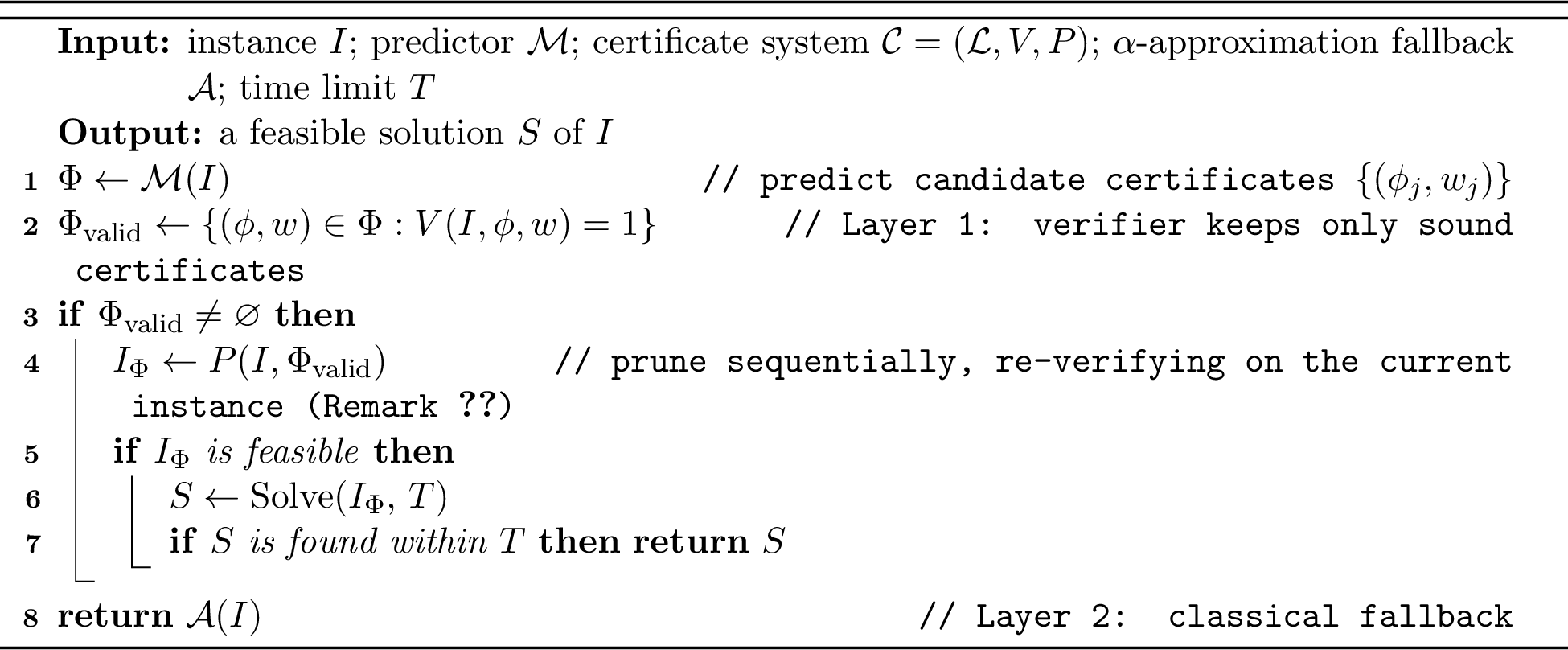
Algorithm 1 implements the inversion with two safety layers. Layer 1 (the verifier) discards every certificate whose witness does not check out, so an erroneous prediction can only be ignored, never acted upon; certificates are applied sequentially, each re-verified on the current reduced instance, unless they preserve every optimum, in which case batching is safe (Remark 1). Layer 2 (the feasibility recheck and the classical fallback \(\mathcal{A}\)) takes over whenever pruning would leave the instance infeasible or the reduced solve exceeds the time limit. Hence the output is always feasible and, by Theorem 3, within \(\max(\rho\,\alpha_{\mathrm{red}},\alpha)\) of optimal, independently of prediction quality; whenever \(\rho\,\alpha_{\mathrm{red}}\le\alpha\) it is never worse than \(\mathcal{A}\) alone. Prediction quality affects only how much is pruned, hence the speedup, not correctness.
Theorem 3 (Robustness upper bound). If \(\mathcal{A}\) is an \(\alpha\)-approximation, \(\mathrm{Solve}\) gives an \(\alpha_{\mathrm{red}}\)-approximation (\(\alpha_{\mathrm{red}}\ge1\)) on the reduced instance, \(V\) is sound, and the adopted pruning, that is the composite of all applied certificates with safety factors multiplying under composition (Theorem 2), is \(\rho\)-safe (Definition 3, with \(c_{\mathrm{fix}}\) accounted for fix–reduce prunings), then Algorithm 1 returns a feasible \(S\) (including any fixed blocks) with \[\label{eq:robust} c(S)\le\max(\rho\,\alpha_{\mathrm{red}},\,\alpha)\cdot\mathrm{OPT}(I).\qquad{(1)}\] In particular if \(\rho\,\alpha_{\mathrm{red}}\le\alpha\) then \(c(S)\le\alpha\,\mathrm{OPT}(I)\): CASP is never worse than the fallback.
Remark 2 (Role of this bound in the rest of the paper). Bound ?? supports most of what follows. It renders the loss family uniformly bounded, hence PAC-learnable with distribution-free samples (Theorem 13, Section 5); it decouples correctness from prediction quality, which we confirm against adversarial certificate injection in E5; and the confidence-filter of Theorem 15 inherits it directly, as its fallback branch is exactly this \(\alpha\)-approximation. Most later safety and learnability statements reduce to ?? .
Theorem 4 (Emergent polynomial solvability). If \(V\) is sound, if the adopted certificates are jointly* OPT-preserving, meaning that some optimum of \(I\) survives the composite pruning, as holds under sequential composition of OPT-preserving certificates (Theorem 2) and, a fortiori, when each certificate preserves every optimum, and if the reduced instance satisfies \(|\mathcal{G}(I_\Phi)|=O(\log|\mathcal{G}(I)|)\), then CASP returns an exact optimum of \(I\) in polynomial time.*
Remark 3. Theorem 4 is what distinguishes CASP from solver presolve [46]: when OPT-preserving certificates compress the effective degrees of freedom to logarithmic size, an NP-hard instance emerges polynomially solvable. Presolve lacks a predictor, lacks \(\rho\)-grading, and provides no such hardness-collapse guarantee. Presolve does implement several of the same underlying reductions, dual fixing for example, so speedup comparisons must control for the solver’s presolve settings; see the protocol note opening Section 8.
3.3 Noise and overhead↩︎
Two practical questions complete the framework. First, what happens to correctness when the predictor is adversarially wrong? Second, when does pruning pay off in wall-clock terms? Theorem 5 answers the first (nothing: the guarantee is prediction-independent), and Proposition 1 states the condition for the second.
Theorem 5 (Noisy-certificate degradation). Suppose each predicted certificate is wrong, i.e.its assertion is false on \(I\), with probability \(\eta\). Then for every \(\eta\in[0,1]\) CASP stays feasible and \(\mathbb{E}[c(S)]\le\max(\rho\alpha_{\mathrm{red}},\alpha)\mathrm{OPT}(I)\): soundness (Definition 2) keeps \(\Phi_{\mathrm{valid}}\) true-only and the feasibility recheck of Algorithm 1 is a second layer, so \(\eta\) affects only the number of valid certificates, hence pruning rate and speedup, not correctness.
Proposition 1 (Net-speedup condition). Let \(T_{\mathcal{M}}\) be the time of one predictor call, \(T_V\) that of one verification, \(k=|\Phi|\) the number of predicted certificates, and let \(T_{\mathrm{red}}\) and \(T_{\mathrm{full}}\) be the exact-solve times of the reduced and of the original instance. When a verified pruning is adopted and the reduced solve completes, CASP runs in \[T=T_{\mathcal{M}}+kT_V+T_{\mathrm{red}}\] against the baseline \(T_{\mathrm{full}}\), with \(T_{\mathcal{M}},T_V\) polynomial; the net speedup is positive iff \(T_{\mathcal{M}}+kT_V<T_{\mathrm{full}}-T_{\mathrm{red}}\), and qualitative when pruning turns an exponentially-blowing instance into a solvable one. When no certificate validates, the overhead \(T_{\mathcal{M}}+kT_V\) is paid on top of the fallback; if \(\mathrm{Solve}\) hits the time limit, the fallback’s running time is additionally incurred.
4 Instantiations↩︎
We instantiate CASP on five structurally diverse problems. Set Cover and Vertex Cover are covering LPs; Facility Location is a two-variable LP with a facility-integral exactness certificate; 0/1 Knapsack is a single-constraint packing maximization; and the Steiner Tree certificate has neither a covering nor a packing LP at its core. Together they confirm that the framework does not live on a single covering-LP skeleton. Each subsection follows the same template: exhibit a polynomial-time verifiable certificate, show it is legal (Definition 4), so that Lemma 1 applies, and either OPT-preserving or \(\rho\)-safe, and then read off the resulting exactness or approximation guarantee through Theorems 1 and 3. What differs across problems is only the certificate; the safety and robustness machinery is shared. Table 1 distinguishes, per certificate, what the verifier actually checks: for most certificates the safety level itself is verified, while for the two complementary-slackness certificates (Set Cover and Facility Location) only the assertion is verified and OPT-preservation rests on the unverifiable assumption Sup (Remark 5).
| Certificate | Assertion verified | Safety level | Safety verified? |
|---|---|---|---|
| SC LP-threshold (\(\tau\le1/f\)) | yes (LP opt.\(+\) \(\tau\)) | \(f\)-safe | yes |
| SC complementary slackness | yes (\(\phi_{CS}\)) | OPT-pres.under | no (conditional) |
| VC NT persistency | yes (half-integral LP) | OPT-preserving | yes |
| FL LP-threshold | yes | \(\Delta\)-safe | yes |
| FL complementary slackness | yes (\(\phi_{\mathrm{close}},\phi_{\mathrm{cut}}\)) | OPT-pres.under | no (conditional) |
| FL facility-integral | yes (\(y^\star\) integral) | OPT-preserving (exact) | yes |
| Knapsack reduced-bound | yes (bound \(+\) incumbent) | OPT-preserving | yes |
| Steiner R1/R2 | yes (degree / Dijkstra) | OPT-preserving | yes |
4pt
4.1 Set Cover↩︎
The certificate is the LP value itself: a set the LP barely uses can be dropped, and the maximum frequency \(f\) sets exactly how aggressively. This yields an \(f\)-safe pruning (Theorem 6) and, under complementary slackness, an OPT-preserving one (Theorem 7). A Set Cover instance is \((U,\mathcal{S},c)\) with \(\mathcal{S}\subseteq2^U\); minimize the cost of a subfamily covering \(U\). Let \(f=\max_{e\in U}|\{S\in\mathcal{S}:e\in S\}|\). The LP relaxation \(\min\sum_S c_S x_S\) s.t.\(\sum_{S\ni e}x_S\ge1\,(\forall e)\), \(x\ge0\) has optimum \(x^\star\) and value \(\mathrm{LP}(I)\le\mathrm{OPT}(I)\).
Lemma 2 (Feasibility preservation). If \(\tau\le1/f\) and we delete all \(S\) with \(x^\star_S<\tau\), the result \(I_\tau\) stays feasible.
Theorem 6 (LP-threshold certificate is \(f\)-safe). For \(\tau\le1/f\), \[\mathrm{OPT}(I_\tau)\le f\cdot\mathrm{OPT}(I);\] with Theorem 3 (\(\rho=f,\alpha_{\mathrm{red}}=1\)), CASP’s ratio is \(\le\max(f,\alpha)\).
Corollary 1 (Exact safety boundary). For \(\tau>1/f\), sets of the LP rounding cover \(\{S:x^\star_S\ge1/f\}\) may be deleted, the \(f\)-bound can fail, and \(I_\tau\) may become infeasible (consider an element covered by \(f\) sets, each with \(x^\star_S=1/f\); any \(\tau>1/f\) deletes them all). Hence \(\tau\le1/f\) is the exact \(f\)-safe boundary; beyond it, any quality gain is empirical with no guarantee. Accordingly, the deployed verifier checks \(\tau\le1/f\) as part of the certificate (Table 1): for \(\tau>1/f\) the certificate is rejected and CASP falls back, so the threshold family \(\mathcal{F}_C\) of Sections 5 and 7 is uniformly bounded over all* \(\tau\in[0,1]\), not merely over the safe range.*
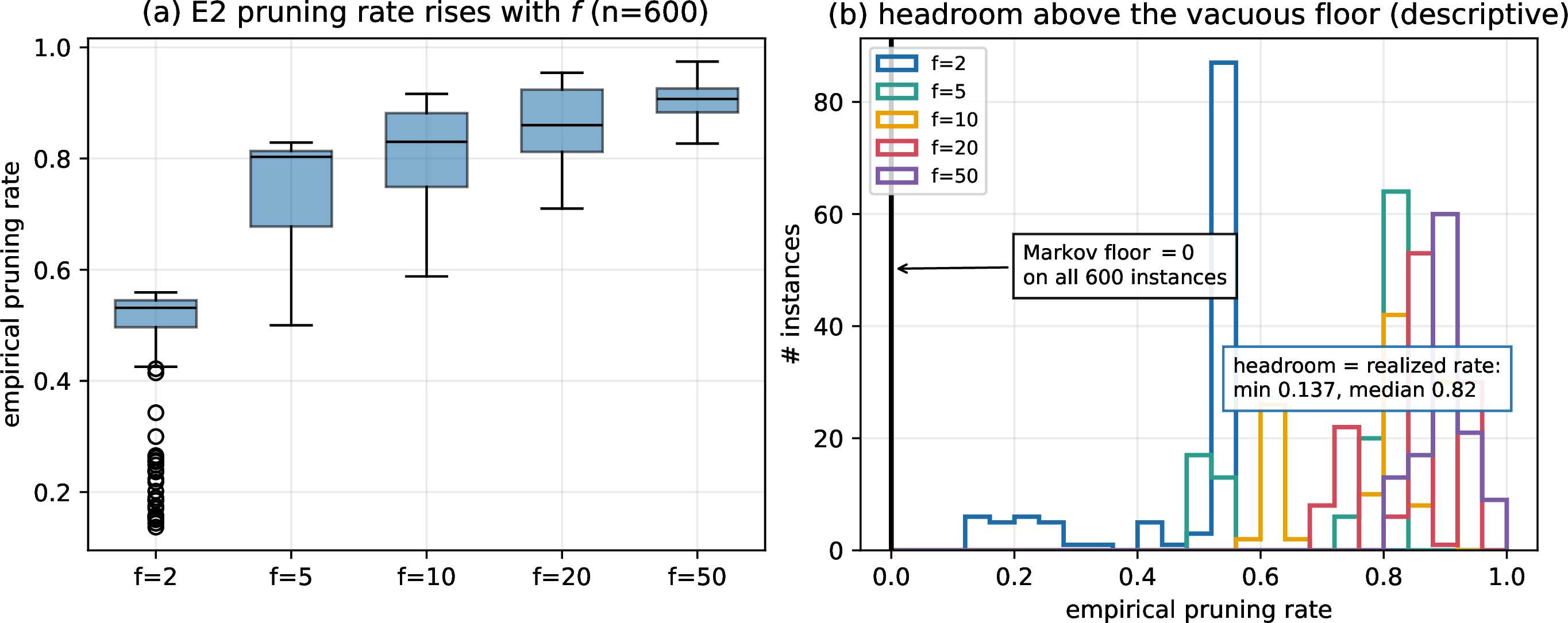
Remark 4 (A counting floor, vacuous in practice). Markov counting (\(\sum_S x^\star_S\ge\tau\cdot\#\{S:x^\star_S\ge\tau\}\)) bounds the survivors by \(\mathrm{LP}(I)/(\tau c_{\min})\) for \(c_{\min}=\min_S c_S>0\), hence a pruning-rate floor \(1-\mathrm{LP}(I)/(\tau c_{\min}|\mathcal{S}|)\). We record it for completeness but do not claim it as a contribution: on all our benchmarks the floor is vacuous (non-trivial on \(0/600\) instances, and still vacuous in a \(|\mathcal{S}|=5000\) stress test; E2), so E2 reports pruning rates descriptively, and a non-trivial, instance-adaptive floor is an open problem.
Theorem 7 (Complementary slackness, conditionally OPT-preserving). Let \((x^\star,y^\star)\) be primal–dual optimal. The assertion \(\phi_{CS}(S)\), namely \(\sum_{e\in S}y^\star_e<c_S\), implies \(x^\star_S=0\). If some integer optimum \(S^\star\) satisfies \(\mathrm{supp}(S^\star)\subseteq\mathrm{supp}(x^\star)\) (condition Sup; e.g.a unique integral LP optimum or an integral LP), then deleting all sets satisfying \(\phi_{CS}\) is OPT-preserving.
Remark 5 (Sup is an assumption, not a verified property). The verifier checks \(\phi_{CS}\), and hence \(x^\star_S=0\), in polynomial time, but condition Sup references an integer optimum and is not polynomially verifiable in general. This certificate’s OPT-preservation is therefore conditional, in contrast to the unconditionally verifiable safety of the NT, facility-integral, reduced-bound, and Steiner certificates; Table 1 records the distinction for every certificate in the paper. Experimentally, E6’s OPT-preserving/approximation split for Set Cover is determined post hoc* against exact optima, and a deployment lacking ground truth can claim only \(f\)-safety for this certificate.*
4.2 Vertex Cover↩︎
The certificate is Nemhauser–Trotter (NT) persistency, recast as a verifiable reduction: it is OPT-preserving (Theorem 8) and, when the half-integral core is logarithmic, upgrades to emergent exact solvability, solving the NP-hard instance optimally in polynomial time (Theorem 9), the sharpest instance of Theorem 4. For \(G=(W,E,c)\) minimize the weight of a vertex set covering all edges. The LP \(\min\sum_v c_v x_v\) s.t.\(x_u+x_v\ge1\,(\forall uv\in E)\), \(x\ge0\) is half-integral: all vertices of the polytope lie in \(\{0,\frac{1}{2},1\}\) (Nemhauser–Trotter [38]).
Theorem 8 (NT persistency is OPT-preserving). Given a half-integral optimum \(x^\star\) with \(P_0=\{x^\star=0\}\), \(P_1=\{x^\star=1\}\), \(P_{1/2}=\{x^\star=\frac{1}{2}\}\), there is a minimum cover \(S^\star\) with \(P_1\subseteq S^\star\) and \(S^\star\cap P_0=\varnothing\); deleting \(P_0\) and fixing \(P_1\) leaves exactly the core \(G[P_{1/2}]\), and \(\mathrm{OPT}(G)=c(P_1)+\mathrm{OPT}(G[P_{1/2}])\).
4.2.1 Triggerable emergent exact solvability↩︎
We turn “emergent solvability” into a provable, triggerable exact algorithm. Call \(G\) \(g\)-NT-decomposable if \(|P_{1/2}|\le g(|W|)\).
Theorem 9 (Named-class exactness). If \(G\) is \((c_0\log n)\)-NT-decomposable (\(n=|W|\), logarithms base \(2\)), minimum weighted vertex cover is solved exactly in \(n^{c_0}\,\mathrm{poly}(n)\) time, and the trigger is one LP solve. Since \(|P_{1/2}|\le2\mathrm{LP}(G)\) for unit costs (in general \(|P_{1/2}|\le2\mathrm{LP}(G)/c_{\min}\)), every unit-cost graph with LP value \(O(\log n)\), and a fortiori with vertex-cover number \(\tau(G)=O(\log n)\), is solved exactly in polynomial time, recovering the LP \(2k\)-kernel as a CASP certificate.
4.3 Facility Location↩︎
Two certificates: an LP-threshold certificate that is \(\Delta\)-safe (Theorem 10), and a facility-integral certificate; whenever the LP opens facilities integrally, a polynomially checkable event, nearest assignment is exactly optimal (Theorem 11). The integrality observation itself is folklore, and the frequent LP-tightness of standard FL benchmarks has been documented since Erlenkotter’s dual ascent [37]; the new element is its packaging as a per-instance verifiable exactness trigger with an emitted optimality proof, which upgrades the weakest branch of the framework to certified-exact. Metric (uncapacitated) Facility Location has a set of facilities (open cost \(f_i\) for facility \(i\)), a set of clients, and distances \(d_{ij}\) satisfying the triangle inequality; open a subset and assign clients to minimize open plus connection cost. The LP uses \(y_i\in[0,1]\) and \(x_{ij}\in[0,1]\): \(\min\sum_i f_iy_i+\sum_{ij}d_{ij}x_{ij}\) s.t.\(\sum_i x_{ij}\ge1\), \(x_{ij}\le y_i\), \(x,y\ge0\). Let \(\delta_j=|\{i:x^\star_{ij}>0\}|\) (the LP support of client \(j\)) and \(\Delta=\max_j\delta_j\).
Theorem 10 (FL LP-threshold certificate is \(\Delta\)-safe). For \(\tau\le1/\Delta\), keeping facilities with \(y^\star_i\ge\tau\) (and their edges) keeps \(I_\tau\) feasible and \(\mathrm{OPT}(I_\tau)\le\Delta\cdot\mathrm{OPT}(I)\); the bound uses no triangle inequality.
The dual has \(u_j\) for coverage and \(w_{ij}\) for \(x_{ij}\le y_i\); we avoid the customary \(\alpha_j,\beta_{ij}\), which are reserved for the approximation factor and the triangle-family parameter. Complementary slackness yields a two-channel certificate \(\phi_{\mathrm{close}}(i):\sum_j w^\star_{ij}<f_i\Rightarrow y^\star_i=0\) and \(\phi_{\mathrm{cut}}(i,j):u^\star_j-w^\star_{ij}<d_{ij}\Rightarrow x^\star_{ij}=0\), OPT-preserving under condition Sup (as in Theorem 7). We now strengthen the weakest branch with a checkable condition that yields exact solutions.
Theorem 11 (Facility-integral certificate: FL becomes exact). Let \((x^\star,y^\star)\) be LP-optimal with \(y^\star\) facility-integral (\(y^\star_i\in\{0,1\}\), a poly-checkable property), \(F^\star=\{i:y^\star_i=1\}\). Then assigning each client to its nearest open facility in \(F^\star\) is an integer optimum; pruning every closed facility and its edges is OPT-preserving, and CASP returns an exact optimum in polynomial time.
This upgrades FL from “\(\Delta\)-safe, OPT-preserving only if unique” to “exact whenever the LP is facility-integral,” triggering the same emergent exactness as NT for VC. In practice the trigger fires; on real ORLIB-cap data the certificate holds on all \(37/37\) instances with zero optimality mismatch (E1). The high firing rate is expected, since LP tightness on these benchmarks is well documented [37]; the empirical contribution is the per-instance checkable proof of exactness that accompanies each solve.
4.4 0/1 Knapsack↩︎
To show the framework is not confined to one covering-LP skeleton we add a problem with the opposite structure: 0/1 Knapsack is a packing, maximization problem with a single constraint. The certificate is classical reduced-cost variable fixing [40], [41], the engine of modern core algorithms [42], recast in our language: a Dantzig bound that forces an item in or out certifies that no optimum flips it, an inclusion/exclusion OPT-preserving pruning (Theorem 12). Items \(i\) have value \(v_i\), weight \(w_i\); capacity \(W\); maximize \(\sum v_i x_i\) s.t.\(\sum w_i x_i\le W\), \(x\in\{0,1\}^n\). Since [8] also study Knapsack, the two prediction interfaces can be contrasted directly on the same problem. Remark 6 records the maximization mirror of the framework used throughout this subsection; in particular a certificate is OPT-preserving if some optimum survives pruning. The negative signal is an exclusion-by-reduced-bound certificate, the CASP reframing of classical knapsack variable fixing. The predictor supplies only a strong feasible incumbent \(z_{\mathrm{low}}\) (value of an exhibited packing, hence \(z_{\mathrm{low}}\le\mathrm{OPT}\)).
Remark 6 (Maximization mirror). Section 3 is phrased for minimization. The mirror used here reads: \(\mathrm{OPT}\) is the maximum feasible value; an \(\alpha\)-approximation returns \(c(S)\ge\mathrm{OPT}/\alpha\); legality replaces cost accounting by value accounting (fixing item \(i\) reduces the capacity by \(w_i\) and credits \(v_i\), so any feasible \(S\) of \(I_\phi\) has \(S\cup\{i\}\) feasible in \(I\) with value \(v(S)+v_i\)); monotonicity becomes \(\mathrm{OPT}(I_\phi)+v_{\mathrm{fix}}\le\mathrm{OPT}(I)\); OPT-preservation is unchanged (some optimum survives); and Theorems 1–4 transfer with the inequalities reversed, by the same proofs.
Theorem 12 (Reduced-bound exclusion/inclusion certificate). Let \(U_i\) be the LP (Dantzig) upper bound subject to forcing \(x_i=1\), and \(U_i^0\) the bound forcing \(x_i=0\), each computable in \(O(n)\) by linear-time weighted-median selection. Let \(z_{\mathrm{low}}\) be the value of an exhibited feasible packing. If \(\phi_{\mathrm{excl}}(i):U_i<z_{\mathrm{low}}\) holds, no optimum contains \(i\), so excluding \(i\) is OPT-preserving; if \(\phi_{\mathrm{incl}}(i):U_i^0<z_{\mathrm{low}}\) holds, every optimum contains \(i\). Both are verified in \(O(n)\).
The surviving items form the knapsack core around the break item; a good incumbent shrinks it, and a verified \(O(\log n)\) core brute-forces (\(2^{O(\log n)}=\mathrm{poly}\)) to an exact optimum with a checkable proof. This is the emergent-exactness mechanism of Theorem 4 (via Remark 6), now on a packing problem with a single constraint and a reduced-cost certificate, structurally disjoint from SC/VC/FL. Against [8] (predicting membership, degrading with error), CASP predicts only a bound used to exclude; correctness is fully decoupled from prediction quality (a bad \(z_{\mathrm{low}}\) simply fails verification).
4.5 Steiner Tree↩︎
The certificate composes two classical reduction tests, recast as verifiable assertions. Steiner Tree asks for a minimum-weight subtree connecting a terminal set (all edge weights strictly positive); its structure is graph connectivity rather than a covering or packing LP. The certificate combines two polynomial-time-verifiable, OPT-preserving reductions from the Steiner preprocessing literature [43], [44], engineered at scale in exact solvers [45]. (R1) Any non-terminal of degree at most one lies in no optimal Steiner tree, since a leaf of an optimal tree is a terminal; the test is applied iteratively. (R2) An edge \((u,v)\) of weight \(w\) is excludable whenever the shortest \(u\)–\(v\) path in \(G\setminus\{(u,v)\}\) costs at most \(w\), because any tree using the edge can be rerouted through the dominating path at no extra cost. The verifier runs one Dijkstra per tested edge. Both tests are applied iteratively, each re-verified on the current reduced graph, since two individually excludable edges may reroute through each other and batching R2 deletions is then unsound; under this sequential discipline the composition is OPT-preserving (Theorem 2, Remark 1).
5 Learnability of Pruning Parameters↩︎
Pruning parameters, the threshold \(\tau\) of Section 4 and later the filter thresholds of Section 6, should not be hand-set per instance but learned from a sample, which raises the question of how many samples suffice. The verifier makes this question well-posed. By capping the loss at a problem constant (Theorem 3) it renders the loss family uniformly bounded, so standard uniform-convergence tools apply. Let instances follow unknown \(\mathcal{D}\), policy \(h_\theta:I\mapsto\Phi\), loss \(\ell_\theta(I)=c(\mathrm{CASP}_\theta(I))/\mathrm{OPT}(I)\in[1,B]\) with \(B=\max(\rho\alpha_{\mathrm{red}},\alpha)\) from Theorem 3. Throughout the learning results, \(K:=\max_I|\mathcal{G}(I)|\) denotes the maximum instance size.
Proposition 2 (Single-parameter pseudo-dimension). For the single-threshold class, \(\ell_\tau(I)\) is piecewise-constant in \(\tau\) with \(\le|\mathcal{G}(I)|\) breakpoints, so \(\mathrm{Pdim}(\mathcal{F})\le O(\log K)\).
Theorem 13 (PAC generalization). If \(\mathrm{Pdim}(\mathcal{F})=d<\infty\) then for \[\label{eq:pacN} N\ge\frac{cB^2}{\varepsilon^2}\Big(d\log\tfrac{B}{\varepsilon}+\log\tfrac1\delta\Big),\qquad{(2)}\] with probability \(\ge1-\delta\) every \(\theta\) satisfies \(\big|\mathbb{E}_\mathcal{D}\ell_\theta-\tfrac1N\sum_i\ell_\theta(I_i)\big|\le\varepsilon\); hence ERM’s \(\hat{\theta}\) is within \(2\varepsilon\) of the in-class optimum.
Theorem 14 (Multi-parameter / combinatorial generalization). Let policies be parameterized by \(\theta\in\mathbb{R}^p\) such that, for every instance, the pruning decisions change across at most \(\Lambda=\mathrm{poly}(K)\) polynomial boundaries of degree \(\le\Delta\) in \(\theta\). Then \(\ell_\theta(I)\) is piecewise-constant on \(\le(8e\Delta\Lambda/p)^p\) cells, and \(\mathrm{Pdim}(\mathcal{F})=O(p\log(\Delta\Lambda))=O(p\log K)\). With the safety-net bound \(\ell_\theta\le B\) preserved for all \(\theta\), the sample complexity is \[N=O\!\Big(\varepsilon^{-2}B^2\big(p\log K\log\tfrac1\varepsilon+\log\tfrac1\delta\big)\Big),\] polynomial in all parameters.
Theorem 14 extends to rich certificate families the boundedness contrast that Section 7 develops: the bare multi-parameter commitment class has the same \(O(p\log K)\) pseudo-dimension yet an unbounded range (Lemma 4 applies verbatim), so the range gap of Theorem 21 persists and is closed only by reinstating a fallback (Theorem 23). E4 tests both regimes: threshold recovery on the benign distribution and gap magnitude on a heavy-tailed one (Section 8).
6 Verifiable Confidence Filtering↩︎
How should an algorithm consume a noisy positive prediction \(\hat{S}\), a candidate solution, without inheriting its errors? The standard safe answer commits the entire prediction and hedges with a classical fallback.
Definition 5 (Min-combiner positive scheme). Let \(\mathrm{fb}\) be a fixed polynomial-time \(\alpha\)-approximation for \(\Pi\). The combiner \(A^+_{\mathrm{comb}}\), on instance \(I\) and prediction \(\hat{S}\), computes a feasible \(S_{\mathrm{pred}}\) from \(\hat{S}\) (commit-and-complete), computes \(S_{\mathrm{fb}}=\mathrm{fb}(I)\), and outputs whichever is cheaper.
The min-combiner is safe, since its loss never exceeds \(\alpha\) (Theorem 23), but coarse; it trusts all of \(\hat{S}\) or none of it. This section shows that a strictly finer operation, enabled by a verifiable per-element confidence signal, provably dominates it, with a margin we compute in closed form.
Let a predictor output \(\hat{S}\subseteq\mathcal{G}(I)\) together with, for each \(i\in\hat{S}\), a confidence \(\sigma_i\in[0,1]\) that is a sound, polynomial-time-verifiable functional of the instance (in our instantiations \(\sigma_i=x^\star_i\), the LP value the verifier already computes). For \(\theta\in[0,1]\) define the confidence filter (CF) \[A^{\mathrm{cf}}_\theta(I,\hat{S})=\min\!\big(\;\mathrm{cost}[\text{commit }\{i\in\hat{S}:\sigma_i\ge\theta\}\text{, then complete}]\;,\;c(\mathrm{fb}(I))\big),\] i.e.commit only the predictions whose verifiable confidence clears \(\theta\), greedily complete to feasibility, and fall back if that is worse; here \(\mathrm{fb}\) is the fixed \(\alpha\)-approximate fallback of Definition 5, whose realized cost satisfies \(c(\mathrm{fb}(I))\le\alpha\,\mathrm{OPT}(I)\) and, unlike \(\alpha\,\mathrm{OPT}(I)\), is computable. Let \(\ell^{\mathrm{cf}}_\theta(I)=A^{\mathrm{cf}}_\theta(I,\hat{S})/\mathrm{OPT}(I)\).
Theorem 15 (Confidence-filter domination). Let \(\ell_{\mathrm{mc}}\) be the loss of the min-combiner of Definition 5 (commit-all, then min with fallback). Then: (i) Containment, consistency, boundedness. \(\ell^{\mathrm{cf}}_0\equiv\ell_{\mathrm{mc}}\); \(\ell^{\mathrm{cf}}_\theta\le\alpha\) for every \(\theta\); and under a perfect prediction \(\ell^{\mathrm{cf}}_\theta(I)=1\) for every \(\theta\le\min_{i\in S^\star}\sigma_i\). (ii) Weak domination.* For every distribution \(\mathcal{D}\), \(\min_\theta\mathbb{E}_\mathcal{D}[\ell^{\mathrm{cf}}_\theta]\le\mathbb{E}_\mathcal{D}[\ell_{\mathrm{mc}}]\). (iii) Strict domination with a computable margin. Part (ii) is strict on explicit families: Theorem 16 computes the asymptotic margin exactly on a Vertex Cover family, and Theorem 17 shows the filter also strictly beats every symmetric prediction-free LP-commit policy (Definition 8); Proposition 3 delineates when strictness is impossible. (iv) Learnability. \(\ell^{\mathrm{cf}}_\theta(I)\) is piecewise-constant in \(\theta\) with \(\le|\hat{S}|\le K\) breakpoints, so \(\mathrm{Pdim}=O(\log K)\) and \(\theta^\star\) is PAC-learnable with \(\tilde{O}(\varepsilon^{-2}\log K)\) samples.*
Remark 7 (Relation to the collapse analysis). Section 7 will show that the sign* of the signal buys nothing once the positive side may min-combine (Corollary 2); certified optimality and bounded loss are supplied by the checking-and-fallback layer, wherever it is installed. Theorem 15 is the guarantee that survives that analysis. Within the positive-signal world, a verifiable confidence signal, the same soundness device CASP is built on, lets a finer policy beat the min-combiner by checking each prediction’s confidence before trusting it, and no fair adversary removes the margin. The next two subsections make it quantitative, and Section 8.10 measures it on two problems and three noise models. The practical rule is to never commit a noisy prediction wholesale but to filter it through the verifiable LP value first. On Vertex Cover this single change brings the cost ratio from the min-combiner’s \(1.32\) down to \(1.03\) at noise level \(0.5\) (Figure 10).*
6.1 An exact margin↩︎
Theorem 15(ii) alone is close to definitional, since the filter family contains the min-combiner at \(\theta=0\); the content lies in the size of the margin and its scaling with noise. We compute both exactly on an explicit family.
Definition 6 (Flip noise). Given an instance with a designated optimum \(S^\star\), the prediction \(\hat{S}\sim F(\eta)\) contains each \(i\in S^\star\) independently with probability \(1-\eta\) and each \(i\notin S^\star\) independently with probability \(\eta\).
Definition 7 (The family \(D_{\beta,C}(n)\)). For \(C>1\) and \(\beta>0\), the Vertex Cover instance \(D_{\beta,C}(n)\) consists of \(n\) disjoint edges \(\{a_i,b_i\}\) with \(c(a_i)=1\), \(c(b_i)=C\), and \(g=\lfloor\beta n\rfloor\) disjoint unit-weight triangles. \(S^\star\) takes every \(a_i\) and two designated vertices per triangle; \(\mathrm{OPT}=n+2g\). The VC LP has a unique optimum: \(x^\star_{a_i}=1\), \(x^\star_{b_i}=0\) on edges and \(x^\star\equiv\frac{1}{2}\) on triangles, so the verifiable confidence is \(\sigma_{a_i}=1\), \(\sigma_{b_i}=0\), \(\sigma_v=\frac{1}{2}\) on triangle vertices. The fallback is LP rounding (\(\{v:x^\star_v\ge\frac{1}{2}\}\), cost \(n+3g\)); completion is greedy with arbitrary tie-breaking.
Theorem 16 (Exact asymptotic margin). On \(D_{\beta,C}(n)\) under flip noise \(F(\eta)\), \(\eta\in[0,1)\): (i)* for every \(\theta\in(\frac{1}{2},1]\) the confidence filter is surely optimal: \(\ell^{\mathrm{cf}}_\theta=1\) deterministically; (ii) the min-combiner satisfies \[\lim_{n\to\infty}\mathbb{E}[\ell_{\mathrm{mc}}] \;=\;1+\frac{\min\!\big\{\eta\big[(C-\eta)+\beta(1-\eta)^2\big],\;\beta\big\}}{1+2\beta};\] (iii) hence the domination margin converges to \[\mathrm{margin}(\eta)\;=\;\frac{\min\!\big\{\eta\big[(C-\eta)+\beta(1-\eta)^2\big],\;\beta\big\}}{1+2\beta},\] which is \(0\) at \(\eta=0\) (consistency), strictly increasing for small \(\eta\), and capped at the fallback gap \(\beta/(1+2\beta)\); the cap is attained at some \(\eta<1\) iff the unsaturated branch \(\eta[(C-\eta)+\beta(1-\eta)^2]\) reaches \(\beta\) on \([0,1)\), for instance whenever \(C>1+\beta\), while for \(C\le1+\beta\) the margin may track the unsaturated branch throughout and need not be monotone in \(\eta\).*
The margin is zero at zero noise, grows with noise, and is capped at the fallback gap. E12 measures this profile (Figure 10), and E14 recomputes the closed form point by point (Section 8.12). At \(\beta=1\) and \(C=2\) the closed form gives \(0.2917\) at \(\eta=0.5\), matching the observed \(0.29\) up to finite-\(n\) and distributional differences of the benchmark family; the cap \(1/3\) is approached only as \(\eta\to1\) at these parameters.
6.2 Prediction is not redundant given the LP↩︎
The filter’s confidence \(\sigma\) is computed by the verifier from the LP, which raises a fair objection. Why not drop the prediction and act on the LP alone? To make \(\sigma\) well defined under degeneracy we canonicalize. The default canonicalization is per-variable: \(\sigma_i:=\max\{x_i:x\;\text{LP-optimal}\}\), computable in polynomial time by one auxiliary LP per variable; the alternative \(\bar\sigma\) reads the analytic center of the optimal face (the limit point of central-path interior-point methods, exactly computable on the symmetric families below), and Remark 9 shows the conclusions hold under both. We quantify over the following class.
Definition 8 (Symmetric LP-commit policies). Fix a canonicalization \(\sigma\) of the LP confidences. A symmetric (prediction-free) LP-commit policy* is a deterministic procedure that commits the set \(\{i:\sigma_i\in A\}\) for a fixed \(A\subseteq[0,1]\), then greedily completes to feasibility, optionally taking the min with a fallback that is itself symmetric: every stage of the pipeline, completion tie-breaking and fallback included, must be invariant under instance automorphisms that preserve \(\sigma\). (We use greedy, which has no ties on the families below; a vertex-returning LP rounding is not symmetric, since which vertex of a degenerate optimal face the solver returns is not a function of \(\sigma\).) Variables with equal confidence are therefore committed or filtered together. The LP-commit policy of the text is \(A=\{1\}\); the \(\mathrm{LP}\theta\) arm of E12\('\) is \(A=[\theta',1]\).*
The next family makes every symmetric LP-commit policy provably suboptimal while the filter, using the prediction only to break the tie on a degenerate optimal face, wins at every noise level.
Definition 9 (The twin-gadget family \(H_{m,n}(\varepsilon)\)). A Set Cover instance with (a) \(n\) pairs: element \(u_i\) coverable by \(A_i=\{u_i\}\) at cost \(1\) or \(B_i=\{u_i\}\) at cost \(C>1\); and (b) \(m\) gadgets: elements \(\{p_j,q_j,r_j\}\) coverable by twin* sets \(T_j,T'_j=\{p_j,q_j,r_j\}\), both of cost \(1+\varepsilon\), or by singletons \(s^1_j=\{p_j\}\) (cost \(1\)), \(s^2_j=\{q_j\}\) (cost \(\frac{1}{2}\)), \(s^3_j=\{r_j\}\) (cost \(\frac{1}{3}\)), with \(\varepsilon\in(0,\frac{3}{8})\). \(S^\star\) takes all \(A_i\) and one designated twin \(T_j\) per gadget; \(\mathrm{OPT}=n+m(1+\varepsilon)\). The optimal LP face on a gadget is the degenerate segment \(\{x_{T_j}+x_{T'_j}=1,\,x_s=0\}\); its analytic center gives \(\bar\sigma_{T_j}=\bar\sigma_{T'_j}=\frac{1}{2}\) and \(\bar\sigma_{s^k_j}=0\), while pairs give \(\bar\sigma_{A_i}=1\), \(\bar\sigma_{B_i}=0\).*
Theorem 17 (Prediction breaks LP degeneracy). On \(H_{m,n}(\varepsilon)\) under flip noise \(F(\eta)\), for every \(\eta\in[0,1)\) and under either canonicalization: every symmetric LP-commit policy (Definition 8) pays at least \(n+\frac{11}{6}m\) surely, since on each gadget it commits both twins or neither, paying \(2(1+\varepsilon)>\frac{11}{6}\) or falling into the harmonic-singleton greedy trap at \(\frac{11}{6}\), while the confidence filter at \(\theta=\frac{1}{2}\) pays \(n+m\big[(1+\varepsilon)+\tfrac{11}{6}\eta(1-\eta)\big]\) in expectation on its commit branch (the min with the realized fallback can only decrease this). Hence \[\mathbb{E}[\mathrm{cost(LP-commit)}]-\mathbb{E}[\mathrm{cost}(A^{\mathrm{cf}}_{1/2})] \;\ge\;m\Big[\tfrac{11}{6}\big(1-\eta(1-\eta)\big)-(1+\varepsilon)\Big] \;\ge\;m\big(\tfrac38-\varepsilon\big)\;>\;0 ,\] with equality in the first step for the branch-only variant against the policy \(A=\{1\}\) under the analytic-center canonicalization, i.e.the filter strictly beats every symmetric LP-commit policy at every* noise level, by a per-gadget margin at least \(\frac{3}{8}-\varepsilon\). The prediction’s role is exactly to break the tie on the degenerate optimal LP face, which no symmetric policy can: any function of the confidences treats \(T_j\) and \(T'_j\) identically.*
Remark 8 (Symmetry is the right boundary). Quantifying over symmetric policies is necessary. A policy that breaks ties by an arbitrary fixed instance order, say committing the lexicographically first twin of each gadget, attains \(\mathrm{OPT}\) on \(H_{m,n}(\varepsilon)\) surely, because the twins there are interchangeable; but it is not a function of the verifiable confidences, and its tie-break is exactly the information a prediction supplies. Randomization is excluded for the same reason: a policy that flips a private fair coin per gadget commits a single twin and attains \(\mathrm{OPT}\) in expectation, but a coin, like a fixed order, is a tie-breaking resource that no function of \(\sigma\) supplies, and Definition 8 quantifies over deterministic maps. The same holds for a combiner whose fallback rounds a solver-returned vertex* of the degenerate face: it too attains \(\mathrm{OPT}\) here, and it too is excluded by Definition 8 for the same reason, because the solver’s vertex choice is a tie-break that no function of \(\sigma\) can express. Theorem 17 therefore isolates a tie-breaking resource: no policy expressible through the LP confidences alone can commit a single twin, while a (possibly learned) prediction can; E13(b) realizes this with a generator tag invisible to the LP. The same reading applies to hypothesis (B1) of Theorem 19.*
Remark 9 (Robustness to the canonicalization). Under the max-canonicalization \(\sigma_i=\max\{x_i:x\;\text{optimal}\}\), both twins get \(\sigma=1\), so the natural policy \(A=\{1\}\) commits both, paying \(2(1+\varepsilon)\) per gadget, and the filter’s advantage against it becomes \((1+\varepsilon)-\frac{11}{6}\eta(1-\eta)\ge1+\varepsilon-\frac{11}{24}>0\) for every \(\eta\); committing neither (\(1\notin A\)) lands in the \(\frac{11}{6}\) trap, as the theorem’s case analysis covers. The separation is therefore not an artifact of how ties are canonicalized; E14 (Section 8.12) validates both canonicalizations against the closed forms, and Section 6.3 shows the construction is one instance of a general decomposable-family principle.
Proposition 3 (Degeneracy limit of confidence filtering). If \(\sigma_i=s\) is constant across \(\hat{S}\) (an LP-opaque* instance, e.g.any VC instance whose NT partition is all-\(\frac{1}{2}\)), then \(\{A^{\mathrm{cf}}_\theta\}_\theta\) contains exactly two policies, the min-combiner for \(\theta\le s\) and prediction-free completion combined with the fallback for \(\theta>s\), so per-element filtering is impossible and strict domination can only come from choosing between those two. Filtering earns its margin precisely on instances with dispersed confidence values.*
Proposition 3 delimits the guarantee and explains the experimental design of E12; the margin lives on instances with mixed LP values. It also motivates predictor-supplied (rather than verifier-computed) confidence, such as calibrated ML confidence checked by the verifier, as the natural extension when the LP is uninformative.
6.2.0.1 Repairing the single-threshold interface: the two-threshold filter.
The single-threshold family has a second, subtler limitation, symmetric to Proposition 3. It contains no policy that ignores the prediction yet still commits high-confidence variables; at \(\theta\) beyond every \(\sigma_i\) it commits nothing and degenerates to the fallback. When the prediction is noisier than the LP is informative, a prediction-free LP-commit policy can therefore beat every \(A^{\mathrm{cf}}_\theta\) (E12\('\), Section 8.11, measures this crossover). The repair, which we call the two-threshold filter CF\(^+\), gives the two signals separate gates: \[A^{\mathrm{cf+}}_{\theta_1,\theta_2}(I,\hat{S}) =\min\!\big(\mathrm{cost}\big[\text{commit }(\hat{S}\cap\{\sigma\ge\theta_1\}) \cup\{i:\sigma_i\ge\theta_2\}\text{, then complete}\big],\,c(\mathrm{fb}(I))\big).\]
Proposition 4 (Two-threshold filter). **(i) Containment.* The family \(\{A^{\mathrm{cf+}}_{\theta_1,\theta_2}\}\) contains the min-combiner (\(\theta_1{=}0\), \(\theta_2\) above every \(\sigma_i\)), every confidence filter \(A^{\mathrm{cf}}_\theta\) (\(\theta_2\) above every \(\sigma_i\)), every threshold LP-commit policy \(\mathrm{LP}\theta\) (\(\theta_1\) above every \(\sigma_i\)), and the fallback; hence \(\min_{\theta_1,\theta_2}\mathbb{E}_\mathcal{D}[\ell^{\mathrm{cf}}_{\theta_1,\theta_2}]\) weakly dominates the best of all four, on every distribution. (ii) Learnability. \(\ell^{\mathrm{cf}}_{\theta_1,\theta_2}(I)\) is piecewise-constant on at most \((|\hat{S}|{+}1)(K{+}1)\) rectangular cells, so \(\mathrm{Pdim}=O(\log K)\), the \(p{=}2\) case of Theorem 14, and \((\theta_1^\star,\theta_2^\star)\) is PAC-learnable with \(\tilde{O}(\varepsilon^{-2}\log K)\) samples. The safety bound \(\ell\le\alpha\) of Theorem 15(i) is inherited unchanged.*
6.3 Decomposable families↩︎
The families \(D_{\beta,C}\) and \(H_{m,n}\) were designed so that the margins close in closed form, and one may reasonably ask how much of Theorems 16 and 17 is an artifact of that design. Only the arithmetic is. Both are equality instances of two general statements about component-decomposable families, whose hypotheses are checkable per component type.
Theorem 18 (Margin on decomposable families). Let \(I_n\) consist of independent copies of finitely many component types \(c\) on disjoint ground sets, \(n_c\) copies of type \(c\) with \(n_c/n\to w_c\), per-component costs bounded by a constant, and noise independent across elements. Suppose for each type \(c\): (A1)* there is \(\theta^\star\) such that on every noise realization the filter’s commit-and-complete cost on \(c\) equals \(\mathrm{OPT}_c\); (A2) commit-all-then-complete has expected cost \(\mathrm{OPT}_c+\varphi_c(\eta)\) on \(c\); and (A3) the fallback costs \(\mathrm{OPT}_c+\delta_c\) on \(c\), deterministically. Then \(\ell^{\mathrm{cf}}_{\theta^\star}=1\) surely, and \[\lim_{n\to\infty}\;\mathbb{E}[\ell_{\mathrm{mc}}]-\mathbb{E}[\ell^{\mathrm{cf}}_{\theta^\star}] \;=\;\frac{\min\{\sum_c w_c\,\varphi_c(\eta),\;\sum_c w_c\,\delta_c\}}{\sum_c w_c\,\mathrm{OPT}_c}.\] Theorem 16 is the instance with types \(\{\mathrm{pair},\mathrm{triangle}\}\), \(\varphi_{\mathrm{pair}}=\eta(C-\eta)\), \(\varphi_{\mathrm{tri}}=\eta(1-\eta)^2\), \(\delta_{\mathrm{pair}}=0\), \(\delta_{\mathrm{tri}}=1\).*
Theorem 19 (Degeneracy advantage on decomposable families). In the same setting add core* types \(g\) and suppose: (B0) on non-core components the filter and every symmetric LP-commit policy (Definition 8) incur equal cost surely; (B1) every symmetric LP-commit policy pays at least \(\mathrm{OPT}_g(1+\delta_g)\) on \(g\), with \(\delta_g>0\); (B2) with probability \(q_g(\eta)\) the filtered prediction commits a cost-\(\mathrm{OPT}_g\) feasible cover of \(g\), and the expected cost of surplus commits on \(g\) is at most \(\rho_g(\eta)\); and (B3) when no cover is committed the filter’s completion on \(g\) costs at most \(\mathrm{OPT}_g(1+\delta_g)\). Then \[\mathbb{E}[\mathrm{cost(LP-commit)}]-\mathbb{E}[\mathrm{cost(filter\;branch)}] \;\ge\;\sum_g n_g\big[q_g(\eta)\,\delta_g\,\mathrm{OPT}_g-\rho_g(\eta)\big],\] strictly positive whenever \(q_g\delta_g\mathrm{OPT}_g>\rho_g\) for some \(g\). Theorem 17 is the instance with a single core type, \(q=1-\eta(1-\eta)\), \(\delta_g\mathrm{OPT}_g=\tfrac{11}6-(1+\varepsilon)\), \(\rho_g=(1+\varepsilon)\eta(1-\eta)\), and there the bound holds with equality.*
The content of the specific families is therefore only that their components verifiably satisfy (A1)–(A3) and (B0)–(B3) with closed-form \(\varphi,\delta,q,\rho\); any other decomposable family with these properties inherits the same conclusions, and E14 validates the two canonical instances over the full parameter grid.
7 Interface Contrasts and Their Collapse↩︎
This section delimits what the certificate interface does and does not buy. Two guarantees separate CASP from the bare membership-vector commitment interface of Definition 10, namely certified optimality (Contrast A) and uniformly bounded loss (Contrast B). Both disappear against a fair adversary that min-combines with the classical fallback of Definition 5 and may run CASP’s own pipeline (Section 7.4). Neither is therefore a complexity separation between paradigms. Each isolates what the checking-and-fallback layer supplies, wherever that layer is installed, and the filtering margin of Section 6 is what no fair adversary removes. We spell the contrasts out nonetheless, both because they calibrate the learning theory through the range factor \(B\) of ?? and because the boundary itself supports the thesis that checking rather than the sign of the signal is the resource.
7.1 A common model↩︎
Fix a minimization problem \(\Pi\) whose optimality-verification language \(\mathrm{OptVer}=\{(I,k):\mathrm{OPT}(I)\ge k\}\) is coNP-complete (true for Vertex Cover, Set Cover, and Facility Location; for the maximization problem 0/1 Knapsack the corresponding language is \(\{(I,k):\mathrm{OPT}(I)\le k\}\), and all statements below transfer mutatis mutandis). Both paradigms below receive \(I\) plus oracle advice and run in polynomial time.
Definition 10 (Bare commitment interface / \(P\)-algorithm). A \(P\)-algorithm \(A^+\) runs in polynomial time; its nontrivial advice is a candidate solution \(\hat{S}\subseteq\mathcal{G}(I)\) (a “what to do” membership vector); it outputs a feasible \(S=A^+(I,\hat{S})\) and nothing else; the interface carries no auxiliary proof object. Advice quality is the Hamming error \(h=|\hat{S}\,\triangle\,S^\star|\) to a nearest optimum. This membership-type interface covers the models of [8] and [9]; edge-type predictions [10] are analogous commitments. The definition restricts the interface, not the computation: a \(P\)-algorithm may run any polynomial computation, including CASP’s own pipeline, a freedom Section 7.4 exercises.
Definition 11 (Poly-time optimality-proof system). A polynomial-time predicate \(\mathrm{Cert}(I,S,\pi)\) with \(|\pi|=\mathrm{poly}(|I|)\) is an optimality-proof system* if (soundness) \(\mathrm{Cert}(I,S,\pi)=1\) implies \(S\) feasible and \(c(S)=\mathrm{OPT}(I)\). An algorithm certifies optimality on \(I\) if it outputs \((S,\pi)\) with \(\mathrm{Cert}(I,S,\pi)=1\); its certified-exact rate on \(\mathcal{D}\) is \(r(\mathcal{D})=\Pr_{I\sim\mathcal{D}}[\text{it certifies optimality on }I]\).*
Certified optimality is the strongest a-posteriori guarantee, since a short and independently checkable proof of optimality accompanies the solution. It is the quantity on which the two interfaces diverge.
Lemma 3 (coNP barrier). If \(\mathrm{OptVer}\) for \(\Pi\) is coNP-hard, no optimality-proof system certifies optimality on every instance unless \(\mathrm{coNP}\subseteq\mathrm{NP}\).
7.2 Contrast A: certified optimality↩︎
We instantiate on Vertex Cover; the construction transfers to any problem with a legal OPT-preserving certificate and a poly-recognizable small-core trigger (Facility Location via Theorem 11). For a weighted graph \(G=(W,E,c)\), let \(x^\star\in\{0,\frac{1}{2},1\}^W\) be a Nemhauser–Trotter half-integral LP optimum with partition \(P_0,P_{1/2},P_1\) (Section 4.2). Let \(\mathcal{K}_{\log}=\{G:|P_{1/2}|\le c_0\log|W|\}\) for a fixed constant \(c_0\), with \(P_{1/2}\) computed from the LP optimum returned by a fixed polynomial-time solver (persistency holds for every half-integral optimum, so membership is solver-relative but the certificate is sound for any choice).
Theorem 20 (Self-certification and universal barrier). **(i) Self-certification.* There is a polynomial-time algorithm, CASP with the NT certificate followed by core enumeration, that on every \(G\in \mathcal{K}_{\log}\) outputs a minimum vertex cover \(S\) together with \(\pi\) such that \(\mathrm{Cert}(G,S,\pi)=1\) for a fixed sound optimality-proof system \(\mathrm{Cert}\); membership \(G\in \mathcal{K}_{\log}\) is decided in polynomial time by one LP solve. (ii) Barrier, binding both paradigms. Unless \(\mathrm{coNP}\subseteq\mathrm{NP}\), no polynomial-time algorithm, CASP included, and no \(P\)-algorithm of Definition 10 even given a perfect prediction \(\hat{S}=S^\star\), outputs, on every VC instance, a feasible cover together with a sound poly-time-checkable optimality proof (Lemma 3). Certified optimality is therefore available only on restricted classes; CASP attains it on all of \(\mathcal{K}_{\log}\) via (i), while the bare interface emits no certificate on any instance, by construction of the interface rather than for complexity reasons, and the same interface equipped with CASP’s checker certifies all of \(\mathcal{K}_{\log}\) (Corollary 2).*
A concrete planted family realizes the self-certification regime distributionally and generates the instances of E7.
Definition 12 (Double-pendant planted model \(G(n,k,H)\)). Pick \(k\) centers, each with two private degree-1 leaves; add an arbitrary graph among the centers; add an independent set of \(n-3k-s\) outer* vertices joined only to centers; implant a hard kernel \(H\) on \(s\) fresh vertices, a vertex-disjoint induced subgraph each of whose LP values is forced to \(\frac{1}{2}\) (e.g.disjoint triangles), attached to centers only.*
Proposition 5 (Planted emergence and interface certification gap). In \(G(n,k,H)\) with \(|H|=s\), and assuming the canonical LP optimum below is the one returned (it is unique): (i) every center is NT-persistent, every leaf and outer vertex lies in \(P_0\), and the NT core is exactly \(H\), so \(|P_{1/2}|=s\); (ii) for \(s=O(\log n)\) CASP solves VC exactly in polynomial time and emits a certified-optimal proof (Theorem 20(i)), while the whole-graph LP optimum is fractional (\(P_{1/2}=V(H)\neq\varnothing\); for \(k=O(s)\) the integrality gap is in addition bounded away from \(1\), the \(H\)-part contributing \(\mathrm{OPT}/\mathrm{LP}=4/3\) on disjoint triangles); (iii) the bare commit-and-complete interface of Definition 10 emits no optimality certificate on any of these instances, since its output carries no proof object, whereas by Corollary 2 the same interface equipped with CASP’s checker certifies all of them (they lie in \(\mathcal{K}_{\log}\)).
Proposition 5 is a distributional illustration of the checking layer rather than a paradigm separation. On inputs whose whole-graph LP optimum is fractional, certified exactness with probability one becomes available exactly when a checking layer is attached to the pipeline, whichever paradigm hosts it.
7.3 Contrast B: bounded loss↩︎
We give a quantitative contrast on the learning axis, in the ERM setting of Section 5: instances are i.i.d.from \(\mathcal{D}\); a policy maps an instance to a prediction; we learn its real parameter by ERM under the cost-ratio loss \(\ell(I)=c(\mathrm{ALG}(I))/\mathrm{OPT}(I)\ge1\). The standard uniform-convergence bound (Theorem 13) for a loss family \(\mathcal{F}\) with range \([1,1+B]\) and pseudo-dimension \(d\) is \[\label{eq:uc} N(\varepsilon,\delta)=O\!\Big(\tfrac{B^2}{\varepsilon^2}\big(d\log\tfrac{B}{\varepsilon}+ \log\tfrac1\delta\big)\Big),\tag{1}\] and the dependence on the range \(B\) is necessary, because for unbounded-range families no distribution-free uniform-convergence bound exists. Let \(\mathcal{F}_C=\{\ell_\tau:\tau\in[0,1]\}\) be CASP’s single-threshold class (Section 4.1); let \(\mathcal{F}^+=\{\ell^+_t:t\in\mathbb{R}\}\) be the structurally identical positive-signal commitment class, given by a learned scorer \(s:\mathcal{G}(I)\to\mathbb{R}\) and the policy that commits every block with score at least \(t\) and then greedily completes to feasibility. The defining difference is the absence of a verifier.
Theorem 21 (Boundedness contrast). **(1)* For Set Cover with maximum frequency \(f\) and fallback factor \(\alpha\), \(\ell_\tau(I)\le B_C:=\max(f,\alpha)\) for all \(\tau\) and all \(I\), and \(\mathrm{Pdim}(\mathcal{F}_C)=O(\log K)\); hence \[\label{eq:Nc} N_C=O\!\Big(\varepsilon^{-2}\max(f,\alpha)^2\big(\log K\log\tfrac1\varepsilon+\log\tfrac1\delta\big)\Big) =\tilde{O}(\varepsilon^{-2}\log K).\tag{2}\] (2) \(\mathrm{Pdim}(\mathcal{F}^+)=O(\log K)\) as well, yet there is a Set Cover family and a scorer (not necessarily consistent) on which \(\ell^+_t\) is unbounded: for every \(M\) some instance has \(\sup_t\ell^+_t(I)\ge M\). Thus \(\mathcal{F}^+\) has no finite range and, by Lemma 4 below, admits no distribution-free uniform-convergence guarantee. Restricting to cost spread \(c_{\max}/c_{\min}\le R\) caps the range at \(\Theta(R)\), making the uniform-convergence bound 1 a factor \(O(R^2)\) larger than 2 ; Theorem 22 shows an \(\Omega(R/\varepsilon^2)\) lower bound, so the spread dependence itself is unavoidable.*
Lemma 4 (Unbounded families admit no distribution-free rate). Let \(\mathcal{F}\) be a loss family with \(\ell_t\ge0\) for which there is a benign instance \(I_0\) with \(B_0:=\sup_t\ell_t(I_0)<\infty\) and, for every \(M\), an instance \(I_M\) with \(\sup_t\ell_t(I_M)\ge M\). Then for every sample size \(N\) there is a two-point mixture \(\mathcal{D}_N\) such that, with probability at least \(0.9\) over \(N\) i.i.d.samples, \(\sup_t\big|\mathbb{E}_{\mathcal{D}_N}\ell_t-\tfrac1N\sum_i\ell_t(I_i)\big|\ge1\). In particular no distribution-free uniform-convergence bound of the form 1 exists for \(\mathcal{F}\).
Theorem 22 (Unavoidable spread dependence). There are a scorer, an absolute constant \(c>0\), and, for every \(R\ge3\) and \(\varepsilon\in(0,\frac{1}{36}]\), two distributions \(\mathcal{D}^\pm\) over Set Cover instances of cost spread at most \(R\) (and maximum frequency \(f=2\)) such that any learning rule that, on each of \(\mathcal{D}^\pm\), outputs from \(N\) i.i.d.samples a threshold \(\hat{t}\) with \(\mathbb{E}[\ell^+_{\hat{t}}]\le\min_t\mathbb{E}[\ell^+_t]+\varepsilon\) with probability at least \(\frac{3}{4}\) must use \(N\ge c\,R/\varepsilon^2\) samples. On the same distributions every CASP threshold \(\tau\in(0,\frac{1}{2}]\) attains \(\ell_\tau\equiv1\) on every realization: the certified class needs no samples where the commitment class needs \(\Omega(R/\varepsilon^2)\), and its rate \(\tilde{O}(\varepsilon^{-2}\log K)\) 2 is \(R\)-independent in general. Whether the \(O(R^2/\varepsilon^2)\) upper bound 1 for the commitment class is tight remains open.
The two classes have identical combinatorial capacity, \(\mathrm{Pdim}=O(\log K)\). The contrast is not expressiveness but boundedness, which the verifier and fallback supply; the loss range is a problem constant on one side and an unbounded, input-dependent quantity on the other. It is the quantitative companion to Theorem 20. Both statements are, however, statements about the interface of Definition 10, and we now show they do not survive a fair adversary.
7.4 A fair adversary collapses both contrasts↩︎
Theorems 20 and 21 restrict the positive side to consuming a membership-vector \(\hat{S}\) through a commit-and-complete rule (Definition 10). That restriction accounts for both results. Grant the positive side two standard and entirely legal powers, the min-combiner of Definition 5 and the right to run in polynomial time whatever computation CASP runs, verifier included, and both contrasts vanish. The boundary itself, rather than a claimed gap, is the result.
Theorem 23 (Combiner collapse of the boundedness contrast). For every instance \(I\) and every prediction, \[\label{eq:comb} c\big(A^+_{\mathrm{comb}}(I,\hat{S})\big)\le\min\big(c(S_{\mathrm{pred}}),\,\alpha\,\mathrm{OPT}(I)\big), \qquad\text{hence}\qquad \ell_{\mathrm{comb}}(I)\in[1,\alpha].\qquad{(3)}\] Thus the combiner class is uniformly bounded by the problem constant \(\alpha\) (matching CASP’s \(\max(f,\alpha)\)); is consistent* (a perfect \(\hat{S}=S^\star\) gives \(\ell_{\mathrm{comb}}=1\)); and has \(\mathrm{Pdim}=O(\log K)\), so by 1 its sample complexity is \(\tilde{O}(\varepsilon^{-2}\log K)\), equal to CASP’s. The \(O(R^2)\) range gap of Theorem 21 disappears.*
Corollary 2 (No fair capability separation). Grant the positive side (a) arbitrary polynomial preprocessing, (b) the min-combiner of Definition 5, and (c) the right to run CASP’s own prune–verify–solve pipeline. Then it matches the negative side on cost, loss range, consistency, sample complexity, and* certified-exact rate. In particular a positive algorithm handed a perfect prediction may simply execute CASP’s pipeline and emit the same checkable optimality proof, so even the certified-optimality advantage of Theorem 20 is an artifact of the commitment interface, not of the sign of the signal.*
Remark 10 (What survives, and why we still build a verifier). Corollary 2 is not purely negative; it isolates the non-definitional content of CASP. First, a single OPT-preserving, polynomially verifiable certificate object unifies NT persistency, complementary slackness, facility-integrality, and reduced-cost fixing as one construction. Second, self-certification is a real engineering guarantee on \(\mathcal{K}_{\log}\) even though a polynomial positive algorithm could in principle reproduce it. Third, the verifier makes correctness prediction-independent (Theorems 3 and 5) without assuming the positive side adopts a combiner. The reframing from “what to do” to “what may be verifiably ignored” is thus a unification and a design principle rather than a complexity separation.
8 Experiments↩︎
The experiments are confirmatory rather than competitive. Each is tied to one proven statement and asks whether its prediction holds and whether its bound is tight. We report fourteen experiment groups (E1–E14, with primed variants E4\('\)/E4\(''\), E6\('\)/E6\(''\), E10\('\), and E12\('\)) spanning the five problems, the interface contrasts, the quantitative filtering theory, and the learnability theory. Table 2 maps each group to the statement it tests and its headline outcome. We first verify the framework itself (correctness, quality sources, learnability, robustness, speedup: E1–E6), then the two heterogeneous problems (E9, E11), then the interface contrasts and their collapse (E7, E8, E10, E10\('\)), and finally the filtering theory and the learned predictors (E12, E12\('\), E14, then E13). All numbers come from one pipeline—SCIP for exact and LP solving,1 time limit \(3600\) s unless stated otherwise, bootstrap \(95\%\) confidence intervals, and an independent reimplementation of every verifier, the \(\mathrm{Cert}\) checker of Theorem 20, so that zero-mismatch claims are audited rather than assumed. Data assets: synthetic Set Cover (\(600\)), Vertex Cover (\(70\)), FL-hard (\(65\)), and Pisinger Knapsack (\(180\)); \(97\) real DIMACS/SNAP graphs, OR-Library SC (\(40\)), ORLIB-cap / UFLLib / TSPLIB Facility Location, SteinLib B-class (\(18\)), and \(62\) adversarial instances.
| # | Experiment / theorem | Headline outcome | Figure/Table |
|---|---|---|---|
| E1 | OPT-preserving exactness (Thm [thm:nt],[thm:flint]) | 0 mismatch; real FL 37/37 exact | Fig. [fig:e1nt] |
| E2 | Pruning-rate profile (descriptive; Rem. [rem:rate]) | rates rise with \(f\); floor vacuous | Fig. [fig:e2full] |
| E3 | Quality-source ablation (Thm [thm:lpsafe]) | prune gain \(\to0\) as \(f\) grows | Tab. [tbl:tab:e3] |
| E4 | Sample complexity (Thm [thm:pac]) | flat landscape; \(0\) excess loss at \(N{=}5\) | Fig. [fig:learn] |
| E4\('\)/E4\(''\) | Multi-parameter PAC (Thm [thm:multipac]) | gap grows with \(p\), vanishes with \(N\) | Fig. [fig:learn] |
| E5 | Robustness (Thm [thm:robust],[thm:noisy]) | safety independent of \(\eta\) | Fig. [fig:e5] |
| E6/E6\('\)/E6\(''\) | Net speedup (Prop [prop:overhead]) | \(0\) loss (OPT-pres.); hard-regime net \(13.7\times\) | Fig. [fig:e6full], Tab. [tbl:tab:e6] |
| E9 | Heterogeneous Knapsack (Thm [thm:knap]) | 0 mismatch; core collapse | Fig. [fig:e9core] |
| E11 | Steiner Tree reductions (§[sec:sec:steiner]) | 15/18 proven optimal, 0 mismatch | Tab. [tbl:tab:steiner] |
| E7 | Certified-optimality contrast (Thm [thm:sepA]) | CASP 30/30; bare interface 0/30 | Fig. [fig:sep](a) |
| E8 | Boundedness contrast (Thm [thm:sepB]) | \(1.0\) vs.\(172.8\times\) (no fallback) | Fig. [fig:sep](b) |
| E10 | Head-to-head vs.[8] | CASP flat; bare commitment degrades | Fig. [fig:sep](c) |
| E10\('\) | Fair three-arm rerun (Thm [thm:collapse]) | combined flat at fallback; bare \(+0.65\) | Fig. [fig:e10fair] |
| E12 | Confidence-filter margin (Thms [thm:cfilter],[thm:margin]) | margin grows to \(0.29\) | Fig. [fig:cf] |
| E12\('\) | Pred.-free baselines; CF\(^+\) (Thm [thm:lponly], Prop [prop:cfplus]) | adv.concentrates on degenerate inst. | Tab. [tbl:tab:e12p] |
| E14 | Exact validation (Thms [thm:margin],[thm:lponly],[thm:genmargin]) | closed forms recomputed, \(O(1/\sqrt n)\) | Figs. [fig:margin],[fig:lponlyfig] |
| E13 | Learned predictors, verified deployment | unv.% loss OOD; verified 0 | Figs. [fig:verified],[fig:learned] |
8.1 E1, E2: correctness invariants↩︎
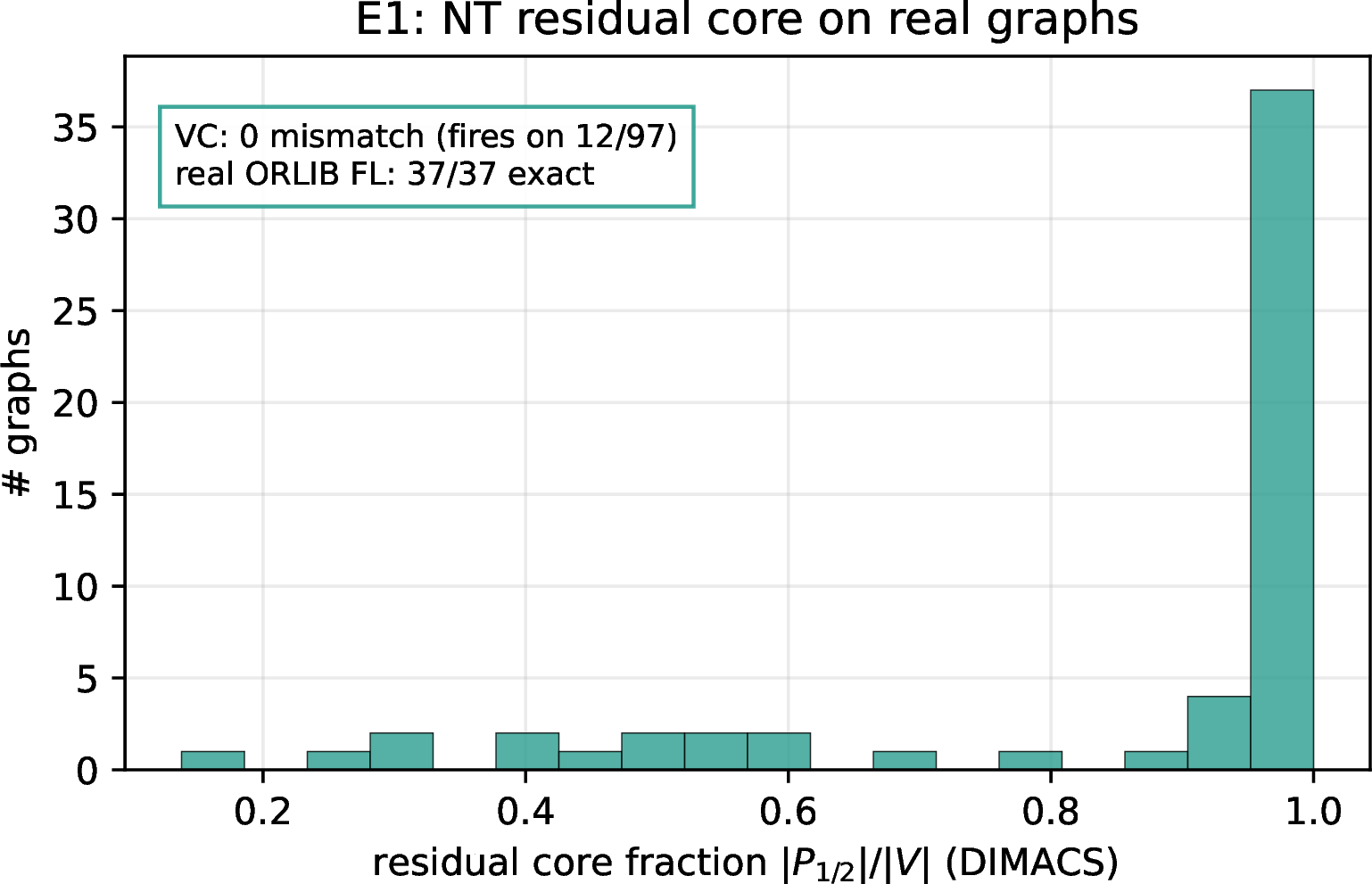
E1 (exactness, Fig. 3). The OPT-preserving certificates incur zero optimality mismatches everywhere they fire. On Vertex Cover, the certificate fires on \(12/97\) of the real DIMACS/SNAP graphs (the NT core is small enough to prune) and every one matches the exact optimum; on the remaining real DIMACS graphs the half-integral core fills the graph (\(|P_{1/2}|\approx|V|\), the histogram in Fig. 3) and the certificate produces no pruning at all rather than fabricating speedup—the behavior a sound certificate must exhibit. On real ORLIB-cap Facility Location the facility-integral certificate (Theorem 11: the LP sandwich in its proof forces exactness) triggers on \(37/37\) instances with \(0\) mismatch, turning the historically weakest branch into a real-data certified-exact result. E2 (pruning-rate profile, Fig. 2). E2 is descriptive rather than a bound validation. The Markov floor of Remark 4 is vacuous on these benchmarks, non-trivial on \(0\) of \(600\) instances and still vacuous at \(|\mathcal{S}|{=}5000\), so plotting violations against it would carry no information. What E2 does establish is the empirical shape. Across all \(600\) synthetic instances the pruning rate rises monotonically with the frequency \(f\) (Fig. 2 (a)), consistent with larger \(f\) letting the LP spread mass over more redundant sets, and Fig. 2 (b) documents how far above the vacuous floor the realized rates sit. A non-trivial, instance-adaptive rate floor remains open.
8.2 E3: sources of solution quality↩︎
The four-arm ablation (greedy \(A\), exact \(B\), prune+greedy \(C\), prune+exact \(D\)) isolates the effect of pruning from the effect of the solver. Table 3 stratifies by frequency \(f\), which resolves a subtlety a blended average would hide. Two invariants hold throughout. The solver upgrade always helps, \(A{-}B>0\), and \(|D{-}B|=0\) at low \(f\) confirms OPT-preservation. The pruning contribution to greedy, however, depends sharply on \(f\): at \(f{=}2\), \(\tau{=}1/f{=}0.5\) prunes so aggressively that the residual is trivialized and greedy already reaches the optimum (C reaches OPT on \(9/10\), so prune gain \(\approx\) solver gain); as \(f\) grows the safe threshold \(1/f\) of Theorem 6 shrinks, the residual stays genuinely hard, and the pruning gain collapses (ratio \(0.99\to0.86\to0.45\to0.16\to0.14\)). The claim that pruning’s value lies in making exact solving feasible rather than in improving quality thus holds in the regime with a non-trivial residual, at moderate and high \(f\); the low-\(f\) windfall is a bonus rather than a contradiction. The stratification also tells a practitioner when to expect pruning alone to suffice.
| \(f\) | prune gain \(A{-}C\) | solver gain \(A{-}B\) | C reaches OPT | \(|D{-}B|\) | prune rate |
|---|---|---|---|---|---|
| 2 | 526.2 | 528.7 | 9/10 | 0.0 | 0.55 |
| 5 | 370.4 | 431.7 | 5/10 | 5.6 | 0.79 |
| 10 | 102.3 | 229.3 | 0/3 | 10.3 | 0.82 |
| 20 | 10.0 | 64.0 | 0/1 | 1.0 | 0.87 |
| 50 | 3.0 | 21.0 | 0/1 | 1.0 | 0.92 |
8.3 E4: learning the thresholds↩︎
E4 (single threshold, Fig. 4 (a)). On the benign training distribution the cost-ratio landscape over \(\tau\) is flat: every threshold in the safe grid ties at mean ratio \(1.0007\), so ERM returns the first minimizer (\(\hat{\tau{=}}0.02\)) and attains zero excess test error from \(N{=}5\) instances. Zero excess error is the prediction, near-trivial here, of the logarithmic pseudo-dimension (Proposition 2; the bound ?? gives the rate 2 ). A landscape with an actual minimum, and the discriminating learning signal, appear on the heavy-tailed distribution of E4\(''\) below. E4\('\) (multi-parameter, Fig. 4 (b), dashed). This measures per-bucket threshold vectors \(\theta\in\mathbb{R}^p\). The loss is uniformly bounded by \(1.14\) for all \(p\in\{2,4,8\}\), the property behind Theorem 14, and the generalization gap, while small, grows with \(p\); at \(N{=}5\), \(p{=}8\) exceeds \(p{=}2,4\), matching \(\mathrm{Pdim}=O(p\log K)\). On this benign distribution (best achievable loss \(\approx1.02\)) the absolute gaps are tiny and the validating signal is the ordering in \(p\). E4\(''\) (heavy-tailed costs, Fig. 4 (b), solid). Re-running the same protocol on \(52\) instances with Pareto(\(1.1\)), size-correlated costs removes that caveat. The best achievable loss rises to \(1.086\); the observed losses stress the certified ceiling, with maximum \(3.02\) against the \(f{=}5\) safety factor entering Theorem 3; and the generalization gap acquires magnitude while keeping both predicted monotonicities, increasing in \(p\) at fixed \(N\) (\(0.0044/0.0088/0.0092\) at \(N{=}5\) for \(p{=}2/4/8\)) and vanishing in \(N\) at fixed \(p\) (\(0.0092\to0.0010\) for \(p{=}8\) as \(N{:}5\to20\)). This is the uniform-convergence shape of Theorem 14.
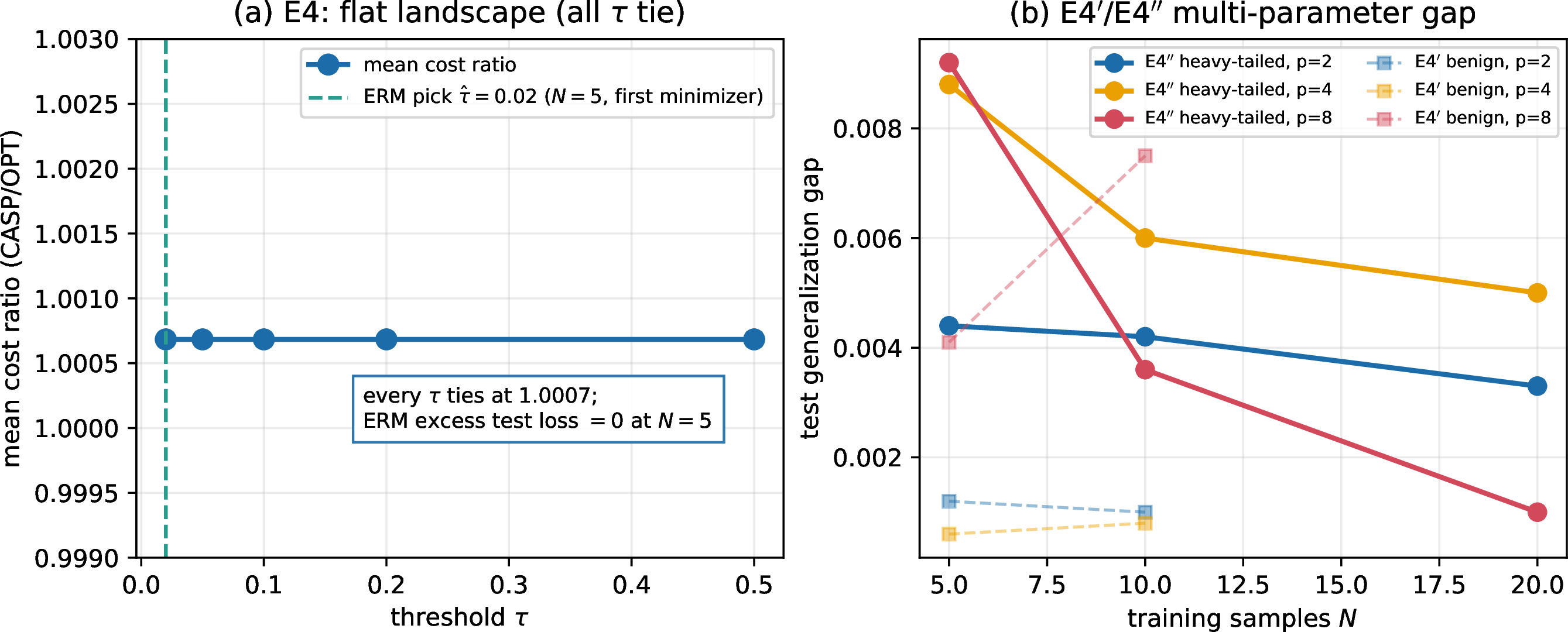
8.4 E5: robustness↩︎
Figure 5 injects certificate noise at rate \(\eta\) and measures the safe rate (output feasible and within the worst-case bound). CASP is safe on \(100\%\) of trials at every \(\eta\) for both Set Cover and Vertex Cover: the two-layer net—verifier rejection of unsound certificates plus the feasibility recheck with classical fallback—makes the worst-case bound ?? , and hence correctness, independent of \(\eta\) (Theorem 5). The contrast with a Balcan-style data-driven configuration that applies the learned threshold without a verifier is instructive. It tracks CASP on clean Set Cover but has no guarantee on adversarial inputs. The experiment isolates the verifier, not the particular threshold value, as the source of the robustness.
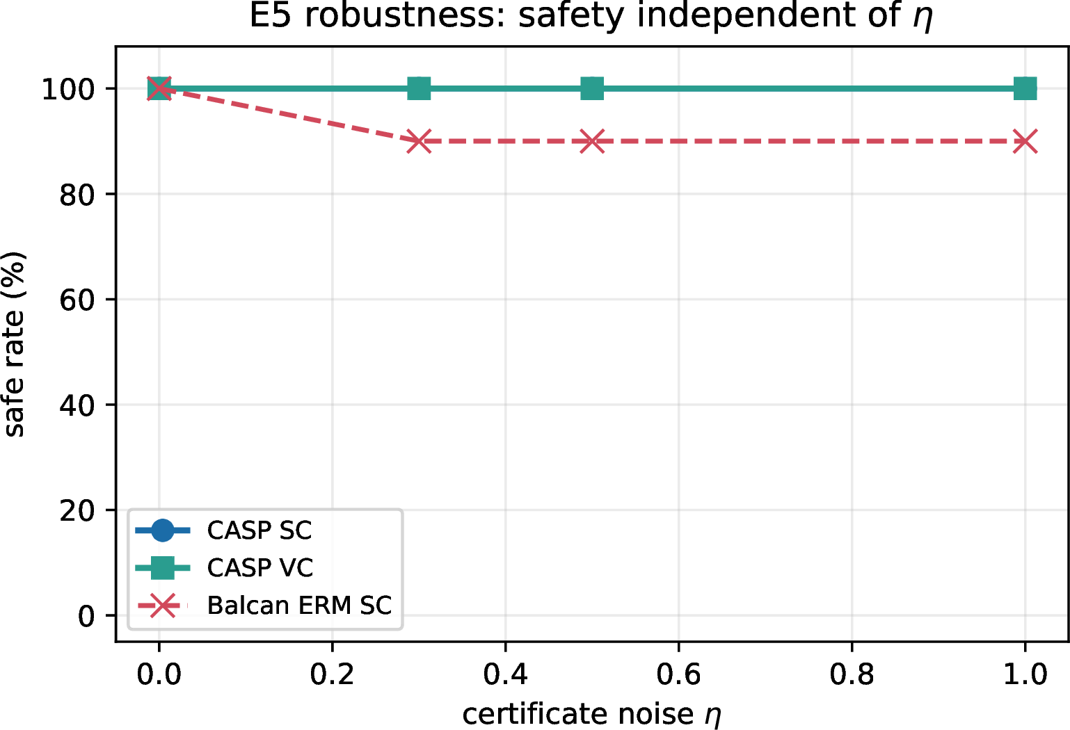
8.5 E6: exact-solving speedup↩︎
Table 4 and Fig. 6 report speedups split by certificate type. The split is determined post hoc against exact optima for the conditional Set Cover certificate (Remark 5); a deployment without ground truth can claim the split only for the certificates whose safety level is itself verifiable (Table 1). E6 covers three regimes under one protocol (SCIP 10.0, default presolve; see the note opening Section 8): classical benchmarks (E6), genuinely hard synthetic instances (E6\('\)), and the rail-scale regime (E6\(''\)).
E6 (benchmarks). The subset of the \(40\) OR-Library instances reported here (\(11+7\)) is the subset on which the exact solver closes both the full and the reduced instance within the time limit; the full manifest ships with the artifact. On real OR-Library Set Cover the OPT-preserving certificates incur zero quality loss, and the \(f\)-approximation-safe cases realize \(0.18\text{--}2.48\%\) cost gaps, two orders of magnitude below the \(f{=}30\) worst-case bound and direct evidence that the bound is loose on real instances. Under the artifact’s original timing protocol these prunings measured as mean \(77.8\times\) (max \(134\times\)) and \(31.7\times\) exact-solving speedups, and synthetic hard Facility Location as \(21.5\times\) (OPT-preserving, \(59\) instances) and \(10.7\times\) (approx, \(6\)), mean \(20.5\times\), max \(189.9\times\). The speedup distributions are skewed (medians \(82.9\times/24.9\times\) for the two Set Cover arms and \(12.4\times/3.1\times\) for FL; Table 4), and the six approximate FL cases have realized gaps of \(0.06\)–\(49\%\), three essentially free and three paying the coarse \(\Delta\)-safe budget, so the split rather than the blend is the informative summary. Figure 6 (b) shows speedup rising with the pruning rate across both problems, as Proposition 1 predicts; the speedup is largest when the solver bottleneck is the number of variables (FL with many facilities, SC with many sets). A protocol audit, however, supersedes the OR-Library wall-clock figures. A \(2\times2\) audit, solver presolve on or off crossed with CASP pruning on or off, run on the scp4x–7x families, shows every such instance solving within seconds under SCIP 10.0 with default presolve, so no wall-clock speedup is measurable there under the audited protocol; the quality figures cross-validate exactly, with mean \(f\)-safe gap \(0.35\%\), maximum \(2.48\%\), and post-hoc OPT-preservation rate \(0.60\), matching the \(11/18\) split. Table 4 therefore documents the audited quality split, its Set Cover timing columns predate the audit and are retained for provenance, and the timing claims of this paper rest on the regimes where exact solving is genuinely hard under the audited protocol, measured next.
E6\('\) (hard synthetic). On \(40\) large synthetic Set Cover instances (\(f{=}10\), \(m{=}2000\); \(300\) s limit per solve) the full instance times out on \(31/40\). On the \(9\) instances both arms solve, the net speedup (LP and pruning time charged to CASP) is mean \(13.7\times\), median \(12.9\times\), max \(21.3\times\), with \(f\)-safe gaps \(\le0.35\%\) (OPT-preserved post hoc on \(1/9\)). Two further instances escape the time limit only after pruning, solving in \(18\)–\(148\) s where the full instance exceeds \(300\) s, the qualitative regime of Proposition 1, and on \(23\) of the \(29\) double-timeouts the pruned run holds the better incumbent at the limit. Pruning therefore buys nothing where modern presolve already solves in seconds and a consistent order of magnitude where exact solving is genuinely hard.
E6\(''\) (rail scale). The largest OR-Library instances, the rail family parsed with a dedicated loader for its transposed format, probe the large-\(f\) extreme. On rail507, with \(507\) rows, \(63{,}009\) columns, and \(f{=}7753\), the LP solves in \(11\) s; the \(\tau{=}1/f\) threshold, despite its nominally useless \(f\)-safe factor, prunes \(\mathbf{99.5\%}\) of the columns because the LP support is tiny; and the pruned instance solves to its optimum, \(176\), in \(7.7\) s versus \(530\) s for the full instance, which SCIP 10.0 proves at the known best \(174\): a realized gap of \(1.15\%\) and, with the \(11\) s LP charged to CASP, a net \(28\times\) end-to-end gain. rail516 behaves the same way (\(19.1\,\mathrm{s}\to0.6\) s, \(184\) vs \(182\), \(1.10\%\)). Rail is an extreme case of the loose-bound phenomenon; the certified \(f\)-safe factor of roughly \(7800\) is vacuous while the realized loss is one percent. Variable pruning works even here; what is missing is a certificate class whose guarantee, not merely its behavior, survives large \(f\).
| Problem | certificate | \(n\) | mean | median | max | quality gap |
|---|---|---|---|---|---|---|
| Set Cover | OPT-preserving | 11 | \(\mathbf{77.8\times}\) | \(82.9\times\) | \(134.3\times\) | \(0\%\) |
| Set Cover | \(f\)-approx-safe | 7 | \(31.7\times\) | \(24.9\times\) | \(57.8\times\) | \(0.18\text{--}2.48\%\) |
| Facility Loc. | OPT-preserving | 59 | \(21.5\times\) | \(12.4\times\) | \(189.9\times\) | \(0\%\) |
| Facility Loc. | approx | 6 | \(10.7\times\) | \(3.1\times\) | \(33.1\times\) | \(0.06\text{--}49\%\) |
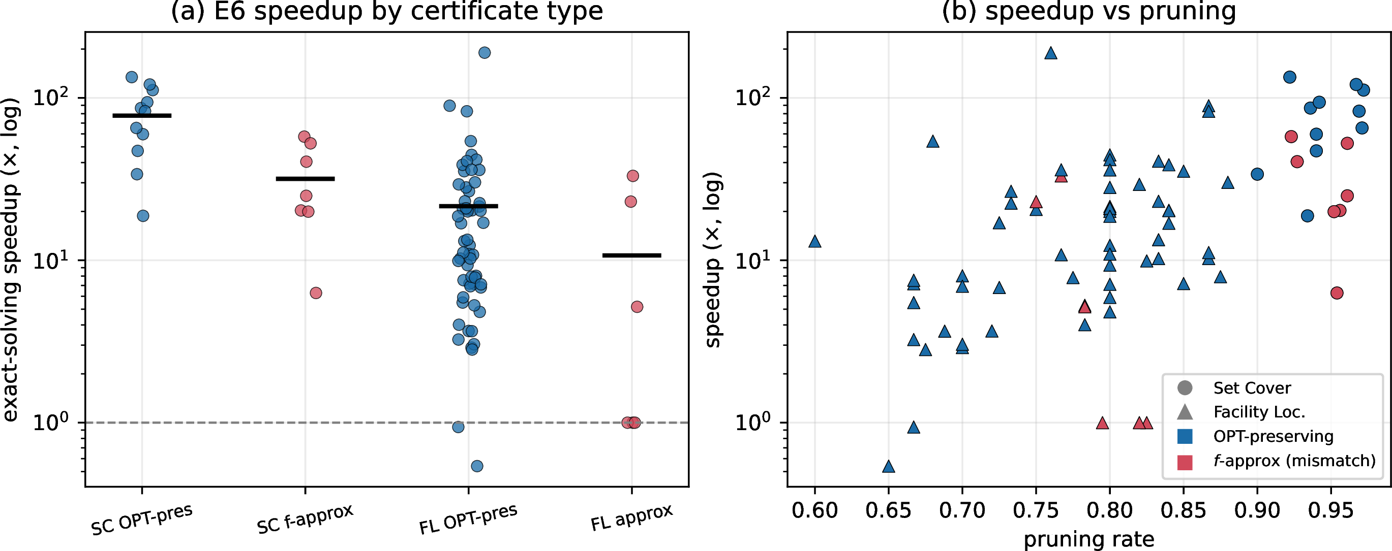
8.6 E9: Knapsack↩︎
Figure 7 demonstrates the framework on 0/1 Knapsack, a packing, maximization, single-constraint problem disjoint from the covering LPs of SC/VC/FL. The reduced-bound certificate (Theorem 12) is correct on all \(35\) instances (seven per Pisinger structural type; the E9/E13 subset manifests ship with the artifact; \(0\) mismatch, audited) and its behavior is structure-dependent in the way the theory predicts. On uncorrelated and spanner instances it collapses the residual core to \(0.14\) and \(0.41\), the emergent-exactness regime; on strongly correlated and subset-sum instances, where the LP gap is tiny and every item sits in the core, it fixes nothing and the core fraction stays at \(1.0\). This mirrors NT on hard graphs and answers the objection that the framework is confined to one LP skeleton.
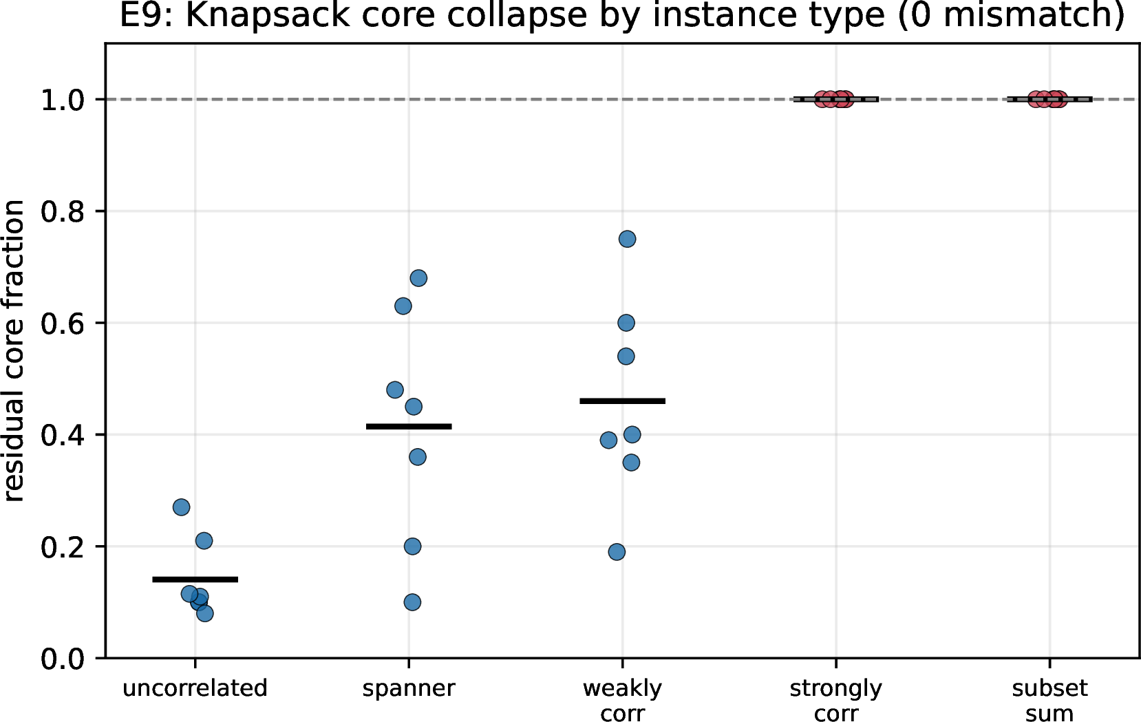
8.7 E11: Steiner Tree↩︎
E11 evaluates the Steiner certificates of Section 4.5 (R1/R2 applied iteratively, re-verified after each deletion) on the SteinLib benchmark. We solve both the original and the reduced instance with an exact multi-commodity-flow ILP (a \(3\)-hour budget). Of the \(18\) B-class instances, \(15\) are solved to proven optimality; on every one of them the certificate is OPT-preserving with \(0\) mismatch (\(\mathrm{opt}(G)=\mathrm{opt}(G_{\text{pruned}})\)), and the value matches the published SteinLib optimum exactly (Table 5). The certificate prunes a mean of \(15.3\%\) of edges (max \(28.6\%\)). The remaining three instances reflect the limits of the generic ILP rather than of the certificate. On B15 the exact solver finds the optimum \(318\) on both graphs yet cannot close the duality gap, and the other incumbents correctly lie above the true optimum. A specialized Steiner solver closes the B-class in milliseconds; the point here is only that the certificate is sound and OPT-preserving wherever exactness can be checked. A second, independent exact solver based on integer row generation closes \(12\) of the instances within budget. It agrees with the multi-commodity-flow solver and with the published SteinLib value on every one of them, which independently confirms OPT-preservation. Steiner Tree thus shows that the framework extends beyond linear-programming structure to a genuinely different combinatorial problem.
| inst | \(|V|\) | \(|E|\) | \(|T|\) | prune % | full OPT | pruned OPT | SteinLib | proven |
|---|---|---|---|---|---|---|---|---|
| B01 | 50 | 63 | 9 | 28.6 | 82 | 82 | 82 | ✔ |
| B07 | 75 | 94 | 13 | 24.5 | 111 | 111 | 111 | ✔ |
| B09 | 75 | 94 | 38 | 16.0 | 220 | 220 | 220 | ✔ |
| B13 | 100 | 125 | 17 | 27.2 | 165 | 165 | 165 | ✔ |
| B14 | 100 | 125 | 25 | 21.6 | 235 | 235 | 235 | ✔ |
| B16 | 100 | 200 | 17 | 5.5 | 127 | 127 | 127 | ✔ |
| B17 | 100 | 200 | 25 | 10.5 | 131 | 131 | 131 | ✔ |
| B18 | 100 | 200 | 50 | 5.5 | 219 | 221 | 218 | — (ILP gap) |
| Aggregate: 15/18 proven optimal, 0 mismatch, all match published SteinLib; mean prune \(15.3\%\); 3 unproven (generic ILP gap, not certificate error). | ||||||||
8.8 E7, E8, E10: interface contrasts↩︎
Figure 8 measures the interface contrasts of Section 7; the capability that survives fair adversaries is measured in Section 8.10. E7 (certified optimality, Fig. 8 (a)). On the planted family \(G(n,k,H)\) of Proposition 5, the realized NT core equals the planted hard core on all \(30/30\) instances, and CASP returns an optimum with a checker-validated proof on all \(30\); every CASP optimum coincides with the SCIP ground truth, all points on the diagonal with zero mismatch. The whole-graph LP optimum is fractional on every instance because the planted core sits at \(\frac{1}{2}\), so no LP-integrality shortcut applies; the emergence comes from the certificate trigger rather than from LP-integral easy inputs. The bare-interface baseline of [8] certifies optimality on \(0/30\) even when its output happens to be optimal — as it must, since its interface returns a solution with no proof object (Proposition 5(iii)); by Corollary 2 the same baseline equipped with our checker would certify all \(30\). E7 therefore isolates the value of the checking layer rather than any computational gap between paradigms.
E8 (boundedness, Fig. 8 (b)). On the cost-spread family, CASP’s worst-case cost ratio is pinned at \(1.0\), strictly under the problem constant \(\max(f,\alpha)\), for every spread \(R\); the structurally identical bare commitment (deliberately run without a fallback, per Definition 10) grows linearly, \(1.17\to2.72\to18.2\to172.8\) as \(R{:}10\to10^4\). Because the two policy classes have identical pseudo-dimension \(O(\log K)\), this gap is not about expressiveness. It is the verifier rendering the loss uniformly bounded, which controls the \(B^2\) factor of the uniform-convergence rate 1 behind the bound 2 . A min-combiner would flatten the curve at \(\alpha\) (Theorem 23); boundedness is supplied by the checking-and-fallback layer, and E8 shows what its absence costs. The empirical \(\Theta(R)\) growth of the unbounded class matches the \(O(R^2)\) uniform-convergence range gap of Theorem 21 and the \(\Omega(R/\varepsilon^2)\) sample-complexity floor of Theorem 22. Note that \(\max(f,\alpha)\) is a problem-family constant rather than a universal one. On families where \(f\) grows, CASP’s own bound grows with it, and the contrast would have to be renormalized.
E10 (head-to-head, Fig. 8 (c)). Sweeping the flip-noise rate \(\eta\) on real Vertex Cover graphs, the ratio of [8] as published (no combiner) rises monotonically from \(1.00\) to \(1.57\) (with widening variance), while CASP stays at \(1.0\): its correctness is decoupled from prediction quality (Theorem 3). The fairness caveat is explicit. A min-combined variant of the baseline flattens near the fallback ratio (Theorem 23), and E10\('\) verifies this point for point on a three-arm rerun (Section 8.9), so E10 measures the decoupling rather than superiority over combined baselines; the comparison against the combiner itself is E12, where the filter wins by the margin of Theorem 16. On the same instances CASP remains certified-optimal on \(70\%\) of this real-VC family, a set distinct from the 97-graph DIMACS/SNAP collection of E1, which explains the different rate; the instance manifest is released with the artifact. The bare baseline certifies none, per its interface. Together the three panels show the checking-and-fallback layer buying decoupled correctness, certified optimality, and bounded-loss learnability; E12 then shows a finer use of the same verifier that no combiner matches.
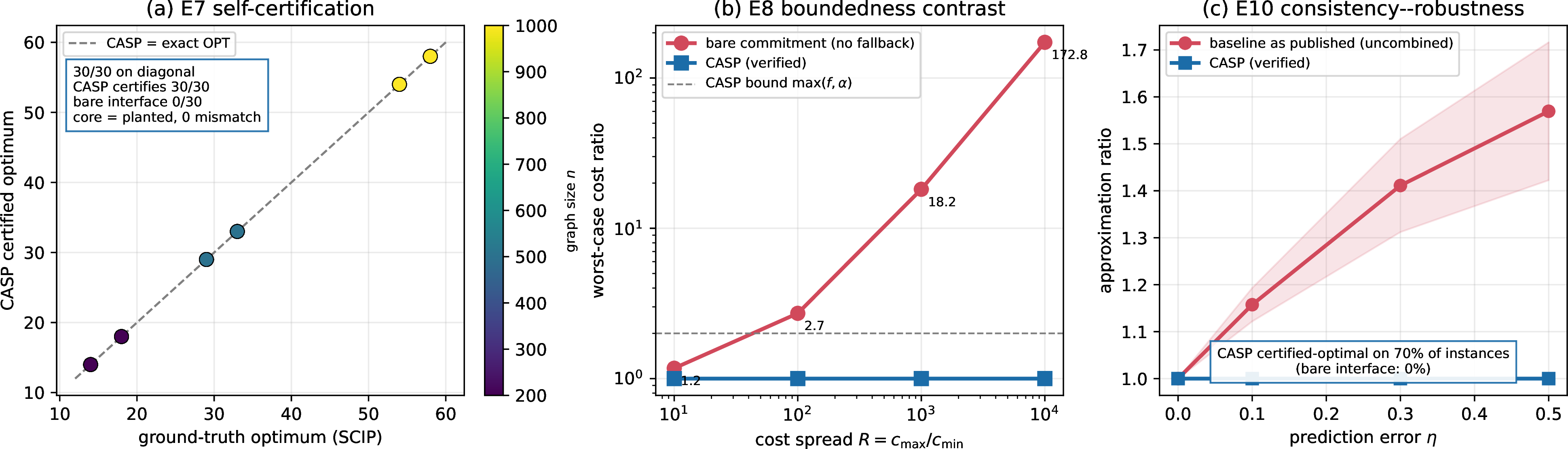
8.9 E10\('\): a fair three-arm rerun↩︎
We apply the fairness standard of Section 7.4 to E10 itself. On \(30\) synthetic VC instances and \(\eta\in\{0,\dots,0.5\}\), the baseline of [8] as published degrades from \(1.000\) to \(1.651\), while the same output min-combined with the LP-rounding fallback is flat at \(1.007\), matching the collapse of Theorem 23 point for point; CASP sits at \(1.002\) with a checker-validated optimality proof on \(93\%\) of instances (Figure 9). E10 and E10\('\) together measure the bare interface’s degradation and the fact that a fallback rather than the sign of the signal removes it. What the combiner still lacks is the certificate, and what neither single-threshold policy supplies is the degeneracy-aware filtering of E12\('\).
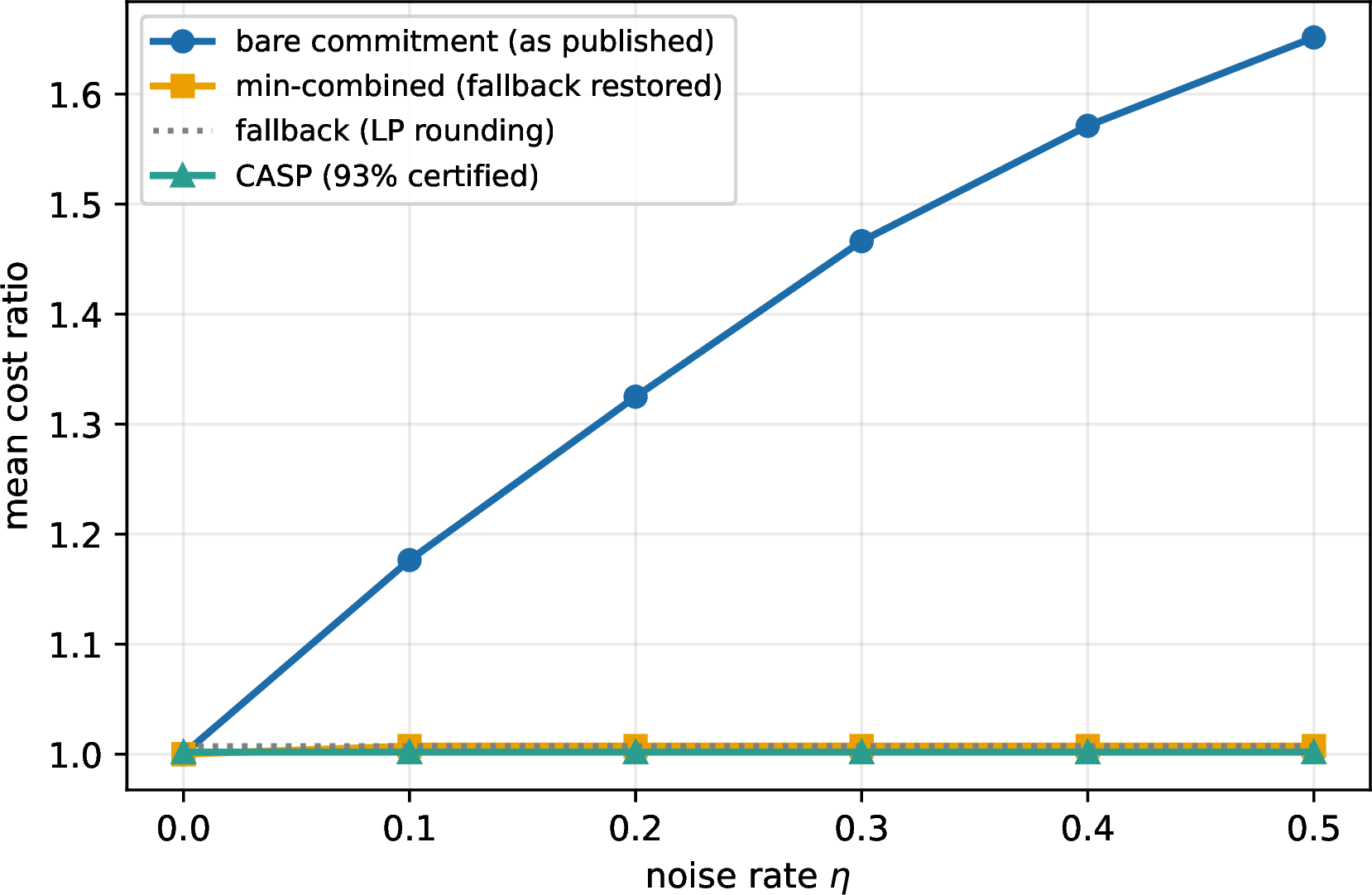
8.10 E12: confidence filtering↩︎
We test Theorems 15 and 16 on Set Cover and Vertex Cover under noisy solution predictions (membership perturbed at rate \(\eta\); confidence \(\sigma_i\) is the LP value the verifier already computes). We compare the min-combiner (commit-all, then min with fallback) against the confidence-filter with a single ERM-learned threshold \(\theta^\star\) (Figure 10 and Table 6). On Set Cover the min-combiner never improves on the fallback, staying at \(1.10\) for every \(\eta\) because committing the noisy prediction wholesale is always worse, while the confidence-filter holds \(1.01\)–\(1.06\). The domination margin of \(0.04\)–\(0.09\) is positive at every noise level and under all three noise models, flip, false-positive-heavy, and drop-heavy, which is the weak domination of Theorem 15(ii). On Vertex Cover the effect is larger and grows with noise. The confidence-filter is nearly noise-invariant at about \(1.03\) for all \(\eta\) while the min-combiner degrades from \(1.04\) to \(1.32\), so the margin rises to \(\mathbf{0.29}\) at \(\eta=0.5\). This is the profile computed on \(D_{\beta,C}\) in Theorem 16, a near-invariant filter, a degrading combiner, and a margin growing toward the fallback gap; at \(\beta=1\) and \(C=2\) the closed form gives \(0.2917\) at \(\eta=0.5\). The learned threshold is a single scalar recovered from \(N\!\approx\!5\) instances with excess loss below \(0.002\). The learning is deliberately cheap; what is being tested is the strict domination of the min-combiner by a verifiable filter.
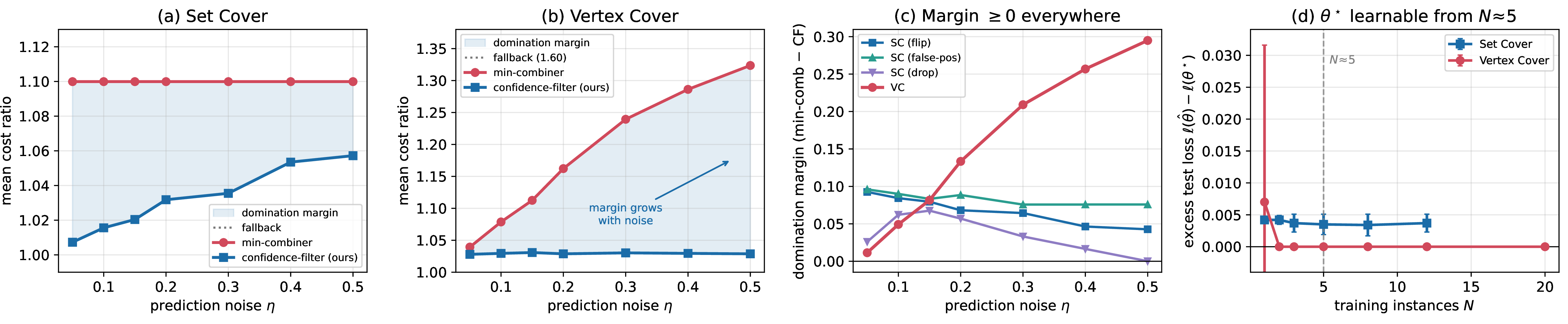
| Problem | \(\eta\) | min-combiner | confidence-filter | margin |
|---|---|---|---|---|
| Set Cover | 0.05 | 1.10 | 1.01 | 0.09 |
| Set Cover | 0.20 | 1.10 | 1.03 | 0.07 |
| Set Cover | 0.50 | 1.10 | 1.06 | 0.04 |
| Vertex Cover | 0.05 | 1.04 | 1.03 | 0.01 |
| Vertex Cover | 0.20 | 1.16 | 1.03 | 0.13 |
| Vertex Cover | 0.50 | 1.32 | 1.03 | 0.29 |
8.11 E12\('\): prediction-free baselines and CF\(^+\)↩︎
E12 compared prediction-consuming policies. E12\('\) adds the missing control and asks whether the filter’s advantage comes from the prediction or from the LP the verifier already solves. On the same distributions and noise models as E12 we add a prediction-free arm \(\mathrm{LP}\theta\) (commit \(\{\sigma\ge\theta'\}\) with \(\theta'\) learned by ERM over a grid containing \(\theta'{=}1\), whose fixed special case is the \(A=\{1\}\) LP-commit policy of Definition 8), and the two-threshold filter \(A^{\mathrm{cf+}}\) of Proposition 4 with jointly learned \((\theta_1,\theta_2)\).
Three findings (Table 7, Figure 11). First, the domination of the min-combiner (Theorems 15, 16) is untouched: \(\mathrm{CF}\le\) min-combiner at every point. Second, the prediction’s added value over the best prediction-free arm has a regime structure. It is positive at low noise, \(+0.013\) at \(\eta{=}0.05\) for Set Cover under flip noise, and negative at high noise, where the single-threshold filter cannot express discarding the prediction while still committing high-LP variables. Stratifying test instances by LP degeneracy, the fraction of fractional \(x^\star\) values, the advantage concentrates where Theorem 17 predicts, on the most degenerate tertile: \(+0.046\) against \(-0.002\) on the least degenerate at \(\eta{=}0.05\), and \(+0.021\) against \(-0.031\) at \(\eta{=}0.30\). On Vertex Cover, \(G(45,0.09)\) with low degeneracy throughout, filter and LP-commit tie at about \(1.03\) for every \(\eta\), the empirical face of Proposition 3. Third, the two-threshold filter repairs the crossover. With a jointly ERM-learned pair it beats the best single-threshold arm strictly at \(18\) of the \(21\) model-noise points, ties at two, and trails by at most \(0.0013\) at the remaining one, drop noise at \(\eta{=}0.5\), within ERM generalization slack. The improvement is a union effect rather than a maximum; under flip noise at \(\eta{=}0.30\) within the CF\(^+\) run, the min-combiner scores \(1.100\), CF \(1.042\), LP\(\theta\) \(1.023\), and CF\(^+\) \(\mathbf{1.018}\).
| \(\eta\) | min-comb | CF | LP\(\theta\) | CF\(^+\) | adv (all) | adv (least deg.) | adv (most deg.) |
|---|---|---|---|---|---|---|---|
| 0.05 | 1.098 | 1.010 | 1.023 | 1.004 | \(+0.013\) | \(-0.002\) | \(+0.046\) |
| 0.15 | 1.100 | 1.019 | 1.023 | 1.008 | \(+0.005\) | \(-0.014\) | \(+0.027\) |
| 0.30 | 1.100 | 1.033 | 1.023 | 1.018 | \(-0.010\) | \(-0.031\) | \(+0.021\) |
| 0.50 | 1.100 | 1.061 | 1.023 | 1.019 | \(-0.037\) | \(-0.058\) | \(-0.018\) |
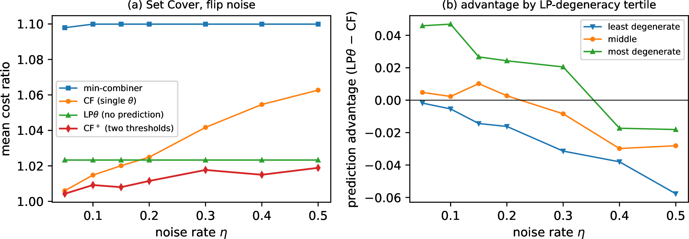
8.12 E14: recomputing the closed forms↩︎
Theorems 16 and 17 make numerical predictions, which admits a strong form of validation, namely Monte-Carlo re-derivation of the closed forms on their own families, grid point by grid point (Figures 12 and 13). Margin (Theorem 16). Across the full grid (\(n\in\{200,1000,5000\}\), \(\beta\in\{0.25,0.5,1,2\}\), \(C\in\{2,5,10\}\), twenty noise levels, \(50\) seeds each, \(720\) configurations in all), the filter is surely optimal in every configuration, a per-realization assertion rather than an average, and the measured min-combiner margin converges to the closed form at the predicted \(O(1/\sqrt n)\) rate, with maximum absolute deviation \(0.033\) at \(n{=}200\), \(0.0065\) at \(n{=}1000\), and \(0.0027\) at \(n{=}5000\). In the saturated regime, \(\beta{=}1\) with \(C\in\{5,10\}\) at large \(\eta\), the measurement is \(0.33333\) against the theoretical \(1/3\). Degeneracy (Theorem 17). Across the corresponding grid on \(H_{m,n}(\varepsilon)\) (\(720\) rows, both \(\sigma\)-canonicalizations of Remark 9), the measured per-gadget margin matches the closed form to at most \(0.018\), is positive at every noise level, and never crosses the proven floors \(\frac{3}{8}-\varepsilon\) (relative-interior) and \(1+\varepsilon-\frac{11}{24}\) (max), with zero violations. E14 is the most direct check in the paper; rather than qualitatively matching the theorems, the experiments recompute their closed forms.
![Figure 12: E14(a): Theorem 16 recomputed by Monte Carlo. Measured min-combiner-vs-filter margins (points, \pm3 s.e.) against the closed form \min\{\eta[(C-\eta)+\beta(1-\eta)^2],\beta\}/(1+2\beta) (curves), per \beta panel at n{=}5000; the dotted line is the fallback-gap cap \beta/(1+2\beta) (an upper bound on the margin, attained only where the unsaturated branch reaches \beta).](/article/2607.14545/fig_margin.png "fig:")
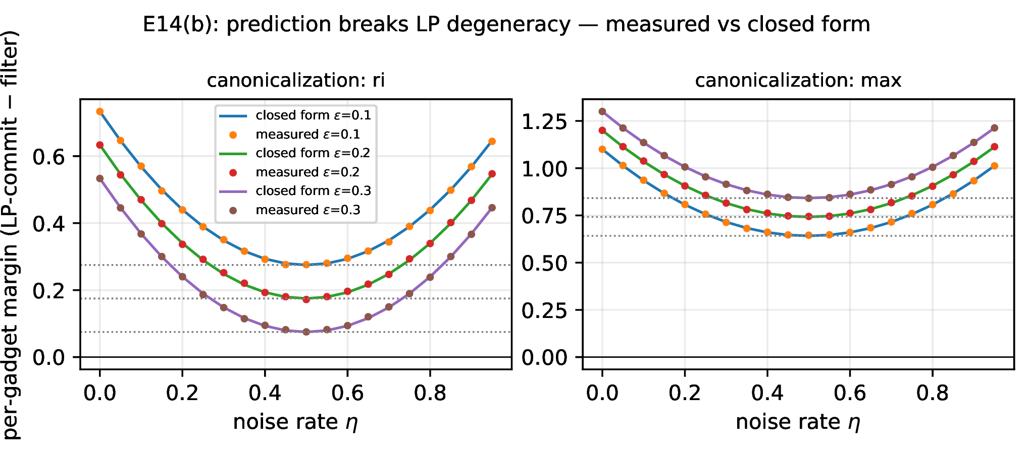
8.13 E13: learned predictors↩︎
All predictions so far were synthetic. E13 trains real predictors and deploys them through the framework, testing the two central claims that the verifier makes imperfect learned predictions safe and that their added value concentrates where Theorem 17 says it must.
8.13.0.1 Verified vs.unverified ML pruning (Figure 14).
A gradient-boosted classifier predicts, per variable, “appears in no optimum” (six combinatorial and LP features; trained on Set Cover \(f{=}5\) instances, respectively on uncorrelated/weakly-correlated Knapsack). The same predictions are deployed in two ways. The unverified deployment deletes every predicted variable, following the ML-problem-reduction template [14], [15]. The verified deployment deletes only the predictions accepted by the CASP verifier, through the \(f\)-safe LP-threshold gate for Set Cover and the OPT-preserving reduced-bound gate of Theorem 12 for Knapsack. In distribution the two deployments are indistinguishable on Set Cover (zero violations either way), while on Knapsack unverified exclusion already forfeits optimality on \(83\%\) of instances, though only by \({\le}0.15\%\). Under distribution shift the magnitudes separate sharply. On Set Cover with \(f{\to}10,20\), unverified pruning produces hard infeasibility on \(10\), \(5\), and \(0\) of \(30\) instances at prediction thresholds \(0.3\), \(0.5\), and \(0.7\), with violation rates, output infeasible or suboptimal, of \(33\%\), \(27\%\), and \(17\%\). The verified arm has zero infeasibility at every threshold, a quality gap of at most \(0.071\%\) inside the \(f\)-safe budget, and essentially all the pruning (\(0.931\) against \(0.932\)). On Knapsack, shifting from uncorrelated to strongly correlated and subset-sum types, unverified exclusion loses optimality on \(\mathbf{97.9\%}\) of instances with value losses up to \(\mathbf{26.2\%}\). The verified arm has zero loss on all \(48\) instances, the OPT-preservation guarantee of Theorem 12 observed without exception, while its acceptance rate collapses to \(0.038\) and \(0.000\) on the correlated types, the same certificate silence as in E9. Verification thus costs coverage, and skipping it costs up to \(26\%\) of the optimal value.
8.13.0.2 A GNN through the filter (Figure 15).
A hand-rolled message-passing GNN predicts VC membership at F1 about \(0.74\)–\(0.77\) from purely combinatorial features, degrees, neighbor statistics, and triangle counts, deliberately excluding the LP values. Committed wholesale, this imperfect predictor costs \(1.154\) in distribution and \(1.331\) out of distribution on \(G(80)\); through CF and CF\(^+\) it is pinned back to \(1.029\) and \(1.037\), tying the LP-commit policy. On this low-degeneracy distribution the learned threshold settles at \(\theta{=}1.0\), so the filter learns to trust only the LP, the behavior Proposition 3 predicts. On a high-degeneracy family the picture inverts. On tagged twin gadgets, the \(H\)-family of Theorem 17 in which the generator marks the historically chosen twin with an observable tag the LP cannot see, a bipartite GNN reaches F1 \(0.911\), and CF\(^+\) attains \(1.137\) against the LP-commit policy’s \(1.288\), the \(11/6\) harmonic trap; the learned advantage is \(+0.151\) per unit OPT, and \(+0.011\) under \(30\%\) tag noise. Together the two panels show a learned predictor earning its margin where the LP is degenerate and the verifier making it deployable everywhere else.
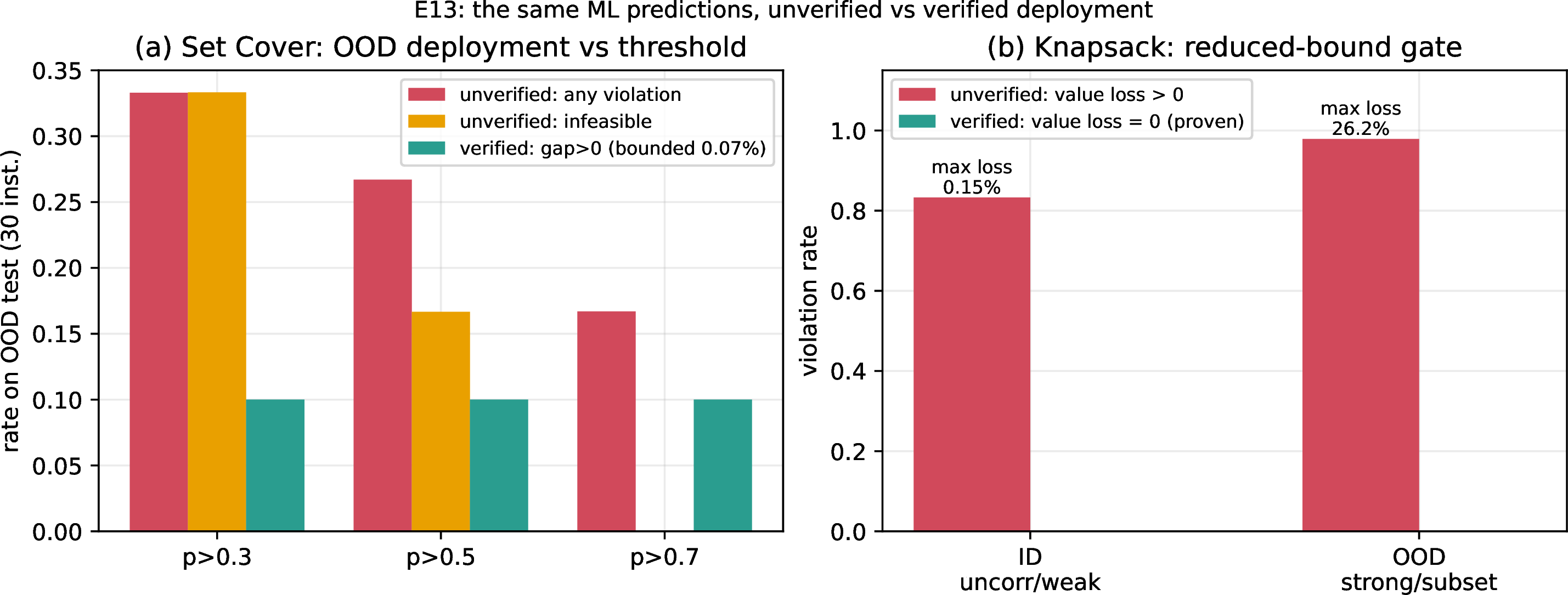
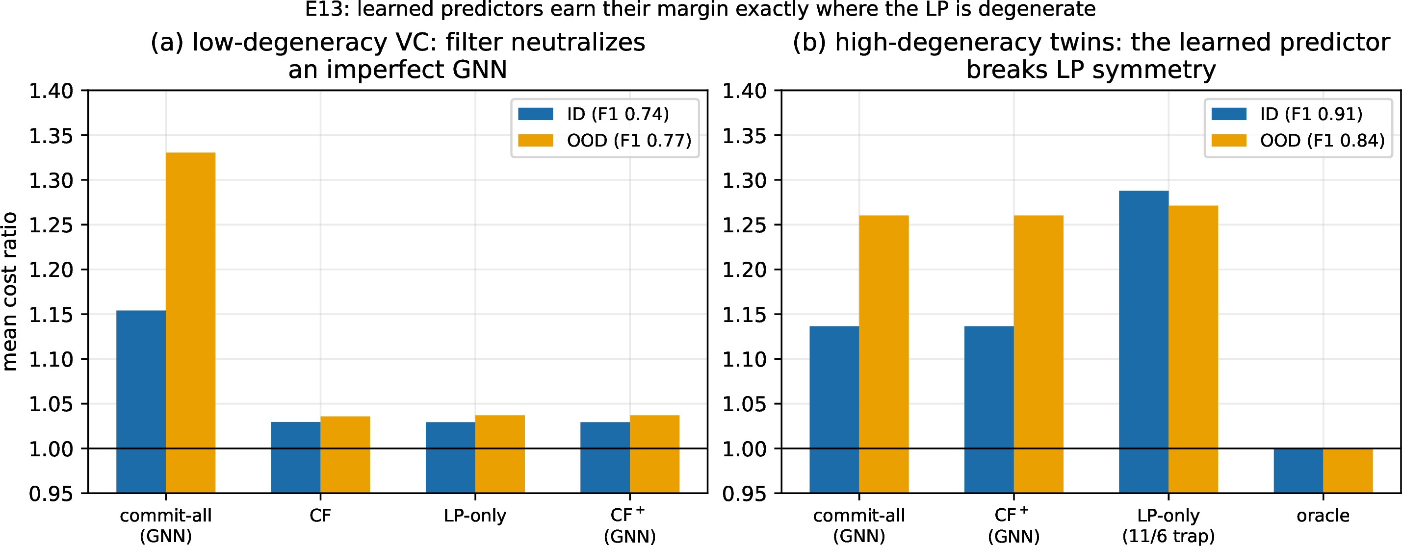
8.14 Discussion and limitations↩︎
The experiments track the theory closely. The interface contrasts appear as predicted and for the predicted, interface-bound reason (E7, E8); prediction-independent safety is confirmed end to end (E5, E10); and the confidence-filter margin has the shape computed in Theorem 16, zero at zero noise, growing, and capped at the fallback gap (E12). The OPT-preserving certificates are never observed to violate optimality (E1, E3, E9), with verification done by an independent checker. Three limitations temper the speedup results. First, the certificates are silent on inputs lacking the relevant structure: NT on dense random and real graphs, firing on \(12\) of \(97\); the Knapsack certificate on correlated instances; the Steiner certificate beyond the ILP-solvable B-class; and the FL threshold on the original CAP library. This is the price of soundness rather than a defect. Second, the headline speedups are largest when the solver bottleneck is the number of variables; at rail scale the certificate still prunes \(99.5\%\) and yields a net \(28\times\) end-to-end gain at a \({\sim}1\%\) realized gap (E6\(''\)), but its certified \(f\)-safe factor is vacuous there; the open problem is not pruning power but a certificate whose guarantee remains meaningful at large \(f\). Third, the proven pruning-rate floor (E2) and the worst-case approximation bounds (E6) are loose on real instances, so the empirical gains exceed what the bounds guarantee; this is good in practice but a sign that the analysis can be tightened. On the planted E7 instances SCIP’s presolve already solves quickly, so the value of CASP there is the checkable optimality proof rather than wall-clock speedup. Speedup is claimed only where exact solving is genuinely hard; the presolve audit and the hard-regime measurements inside E6/E6\('\) delimit exactly where that is. On validity, results use one solver, SCIP 10.0 via PySCIPOpt 6.2.1, and the E4\('\) distribution is benign, so there we present only the ordering in \(p\); E4\(''\) removes this caveat on a heavy-tailed distribution. A further limitation follows from Proposition 3 and is confirmed by E12\('\). The confidence filter earns its margin only where the LP confidence is dispersed; on the low-degeneracy VC distribution the prediction adds nothing over LP-commit, and at high noise the single-threshold filter loses to a prediction-free arm unless upgraded to the two-threshold filter of Proposition 4. This motivates predictor-supplied, verifier-checked confidence as future work. None of these caveats touch the boundedness theory, the collapse analysis (Section 7.4), or the quantitative filtering guarantees (Theorems 16, 17), which are the paper’s core contribution and rest on exact computations on explicit constructions rather than on favorable instances.
9 Conclusion↩︎
CASP inverts the information flow of prediction-augmented algorithms, asking the predictor for verifiable certificates of what may be ignored rather than what to do, and thereby brings predictions to offline NP-hard approximation with prediction-independent safety. The central results are quantitative and belong to the checking layer. The verifier makes the learnable loss class uniformly bounded where the bare interface provably admits no distribution-free rate (Theorem 21, Lemma 4); a verifiable confidence filter dominates the min-combiner with an exactly computed margin, zero at zero noise and growing with small noise (Theorem 16); and the prediction is provably not redundant given the LP, since its role is to break the tie on a degenerate optimal face, which no symmetric LP policy can do (Theorem 17). We have been equally explicit about what checking does not buy. Certified optimality and the boundedness gap are interface contrasts that a fair min-combiner adversary matches (Section 7.4), and the filter degenerates on LP-opaque cores (Proposition 3). Empirically the prediction’s advantage concentrates on LP-degenerate instances as Theorem 17 predicts, and the two-threshold filter of Proposition 4 carries it across the noise range (E12\('\)).
With trained predictors the same pattern appears end to end. An imperfect GNN is neutralized by the filter on low-degeneracy inputs and earns \(+0.15\) on degenerate ones, and unverified ML pruning loses up to \(26\%\) under distribution shift where the verified deployment loses nothing (E13). We instantiated the framework on five structurally diverse problems by recasting classical reductions as verifiable certificates, made emergent exact solvability a triggerable algorithm on a named class and a planted distribution, and generalized the PAC theory to multi-parameter certificate classes. Several directions remain open: certificate classes whose guarantees survive large frequencies, as in the rail regime of E6\(''\) where behavior is excellent but the \(f\)-safe bound is vacuous; OPT-preserving certificates for non-integral Set Cover; predictor-supplied, verifier-checked confidence for LP-opaque cores; and learned, adversarially robust certificate generators evaluated against unverified ML problem reduction [14], [15].
9.0.0.1 Code and data availability.
All experiment code, the synthetic-instance generators together with the generated instances (Set Cover, Vertex Cover, Facility Location, Knapsack, and the adversarial set), per-instance manifests and checksums for every benchmark used (OR-Library Set Cover and rail, DIMACS/SNAP graphs, ORLIB-cap / UFLLib / TSPLIB Facility Location, SteinLib B-class, Pisinger Knapsack), the reimplemented positive-signal baseline of [8] used in E7/E10/E10\('\), solver configurations (SCIP 10.0 via PySCIPOpt 6.2.1, seeds included), the independent verifier reimplementation, and the \(\mathrm{Cert}\) checker of Theorem 20 are packaged as a versioned artifact, available at https://github.com/llfuture/casp. The public benchmarks remain available from their cited sources; the artifact mirrors instance files only where the source license permits and otherwise ships download manifests with checksums.
10 Proofs↩︎
The statements appear in the main text; each proof is given below in its own subsection.
10.1 Proof of Lemma 1↩︎
Let \(S\) be optimal for \(I_\phi\). By Definition 4, \(S\cup F\) is feasible in \(I\) with cost \[c(S)+c_{\mathrm{fix}}=\mathrm{OPT}(I_\phi)+c_{\mathrm{fix}}\ge\mathrm{OPT}(I).\] Block pruning has \(F=\varnothing\), \(c_{\mathrm{fix}}=0\), and \(S\) itself is feasible in \(I\). \(\square\)
10.2 Proof of Theorem 1↩︎
\(\ge\) by Lemma 1. \(\le\), block case: an optimum \(S^\star\subseteq\mathcal{G}(I_\phi)\) is feasible in \(I_\phi\) (it covers \(U(I_\phi)=U(I)\)) at cost \(\mathrm{OPT}(I)\), so \(\mathrm{OPT}(I_\phi)\le\mathrm{OPT}(I)\).
\(\le\), fix–reduce case: Definition 3(1) supplies an optimum \(S^\star\supseteq F\) with \(S^\star\setminus F\subseteq\mathcal{G}(I_\phi)\) and \(S^\star\setminus F\) feasible in \(I_\phi\), at cost \(c(S^\star)-c_{\mathrm{fix}}=\mathrm{OPT}(I)-c_{\mathrm{fix}}\); hence \(\mathrm{OPT}(I_\phi)+c_{\mathrm{fix}}\le\mathrm{OPT}(I)\), and Lemma 1 makes it an equality. (For the NT certificate the feasibility clause is exactly the structure lemma inside the proof of Theorem 8: every edge of the core has both ends in \(P_{1/2}\), so it is covered by \(S^\star\setminus P_1\).) \(\square\)
10.3 Proof of Theorem 2↩︎
We have \(\mathrm{OPT}(I_{\phi_1})\le\rho_1\mathrm{OPT}(I)\), hence \[\mathrm{OPT}(I_{\phi_1,\phi_2})\le\rho_2\,\mathrm{OPT}(I_{\phi_1})\le\rho_1\rho_2\,\mathrm{OPT}(I);\] the chain \(\mathcal{G}(I_{\phi_1,\phi_2})\subseteq\mathcal{G}(I_{\phi_1})\subseteq\mathcal{G}(I)\) transfers feasibility. For fix–reduce prunings the same chain holds with the fixed costs carried along: \(\mathrm{OPT}(I_{\phi_1,\phi_2})+c^{(2)}_{\mathrm{fix}}\le\rho_2\,\mathrm{OPT}(I_{\phi_1})\), hence, using \(\rho_2\ge1\), \(\mathrm{OPT}(I_{\phi_1,\phi_2})+c^{(1)}_{\mathrm{fix}}+c^{(2)}_{\mathrm{fix}} \le\rho_2\big(\mathrm{OPT}(I_{\phi_1})+c^{(1)}_{\mathrm{fix}}\big)\le\rho_1\rho_2\,\mathrm{OPT}(I)\).
Sequential OPT-preservation (block pruning): Theorem 1 applied twice gives \(\mathrm{OPT}(I_{\phi_1,\phi_2})=\mathrm{OPT}(I_{\phi_1})=\mathrm{OPT}(I)\); any optimum of \(I_{\phi_1,\phi_2}\) is feasible in \(I\) (block prunings leave \(U\) unchanged) at cost \(\mathrm{OPT}(I)\), hence is an optimum of \(I\) contained in \(\mathcal{G}(I_{\phi_1,\phi_2})\), which is OPT-preservation of the composite.
Simultaneous application preserving the same \(S^\star\): then \(S^\star\subseteq\mathcal{G}(I_{\phi_1,\phi_2})\) and Theorem 1 applies. \(\square\)
10.4 Proof of Theorem 3↩︎
Branch one (valid certificate, reduced instance feasible, \(\mathrm{Solve}\) succeeds): let \(S_0\) be the reduced solution and \(S=S_0\cup F\) the returned solution (\(F=\varnothing\), \(c_{\mathrm{fix}}=0\) for block pruning). Then \(c(S_0)\le\alpha_{\mathrm{red}}\,\mathrm{OPT}(I_\Phi)\) and, using \(\alpha_{\mathrm{red}}\ge1\) and \(\rho\)-safety in the form \(\mathrm{OPT}(I_\Phi)+c_{\mathrm{fix}}\le\rho\,\mathrm{OPT}(I)\) (Definition 3), \[c(S)=c(S_0)+c_{\mathrm{fix}}\le\alpha_{\mathrm{red}}\,\mathrm{OPT}(I_\Phi)+c_{\mathrm{fix}} \le\alpha_{\mathrm{red}}\big(\mathrm{OPT}(I_\Phi)+c_{\mathrm{fix}}\big)\le\rho\,\alpha_{\mathrm{red}}\,\mathrm{OPT}(I);\] \(S\) is feasible in \(I\) by legality (Definition 4).
Branch two (no valid certificate, infeasible after pruning, or timeout): return \(\mathcal{A}(I)\), \(c(S)\le\alpha\mathrm{OPT}(I)\). Take the max. \(\square\)
10.5 Proof of Theorem 4↩︎
Joint OPT-preservation means some optimum of \(I\) survives the composite pruning, so Theorem 1, applied to the composite, gives \(\mathrm{OPT}(I_\Phi)=\mathrm{OPT}(I)\) (block case; the fix–reduce identity carries \(c_{\mathrm{fix}}\)); the hypothesis is discharged either by the sequential branch of Theorem 2 or because each certificate preserves every optimum. The number of feasible solutions of \(I_\Phi\) is at most \[2^{|\mathcal{G}(I_\Phi)|}=2^{O(\log|\mathcal{G}(I)|)}=\mathrm{poly}(|\mathcal{G}(I)|);\] brute force (or exact IP) finds the optimal \(S^\star\) of \(I_\Phi\) in polynomial time (each subset is checked by the polynomial-time feasibility predicate of Section 3). \(S^\star\) is feasible in \(I\) at cost \(\mathrm{OPT}(I_\Phi)=\mathrm{OPT}(I)\); for fix–reduce certificates return \(S^\star\cup F\), whose cost is \(\mathrm{OPT}(I_\Phi)+c_{\mathrm{fix}}=\mathrm{OPT}(I)\) by Theorem 1. \(\square\)
10.6 Proof of Theorem 5↩︎
Wrong certificates fail the verifier; infeasible pruning triggers fallback (\(\le\alpha\mathrm{OPT}\)); valid certificates fall under Theorem 3 branch one (\(\le\rho\alpha_{\mathrm{red}}\mathrm{OPT}\)). Take the max; the bound is independent of \(\eta\). \(\square\)
10.7 Proof of Lemma 2↩︎
For each element \(e\), \[\sum_{S\ni e}x^\star_S\ge1 ,\] and at most \(f\) sets contain \(e\), so by averaging some \(S\ni e\) has \(x^\star_S\ge1/f\ge\tau\) and survives; \(e\) remains covered. \(\square\)
10.8 Proof of Theorem 6↩︎
Classical LP rounding. Let \(\hat{S}=\{S:x^\star_S\ge1/f\}\); by Lemma 2 it covers \(U\). Its cost satisfies \[\label{eq:fsafe} c(\hat{S})=\!\!\sum_{S:\,x^\star_S\ge1/f}\!\!c_S \;\le\;f\!\!\sum_{S:\,x^\star_S\ge1/f}\!\!c_S x^\star_S \;\le\;f\sum_S c_S x^\star_S=f\,\mathrm{LP}(I)\le f\,\mathrm{OPT}(I).\tag{3}\] Every \(S\in\hat{S}\) has \(x^\star_S\ge1/f\ge\tau\), so it survives in \(I_\tau\); hence \(\mathrm{OPT}(I_\tau)\le c(\hat{S})\le f\mathrm{OPT}(I)\). \(\square\)
10.9 Proof of Theorem 7↩︎
Complementary slackness gives \[x^\star_S>0\;\Longrightarrow\;\sum_{e\in S}y^\star_e=c_S ,\] whose contrapositive gives \(\phi_{CS}(S)\Rightarrow x^\star_S=0\), i.e.the pruned sets lie outside \(\mathrm{supp}(x^\star)\). Under Sup the integer optimum \(S^\star\subseteq\mathrm{supp}(x^\star)\) uses no pruned set, so \(S^\star\subseteq\mathcal{G}(I_{\phi_{CS}})\). (“Unique LP optimum” alone is insufficient: a unique but fractional optimum only preserves the LP value, not an integer optimum; Sup is required.) \(\square\)
10.10 Proof of Theorem 8↩︎
(i) Half-integrality [38] yields the partition.
(ii) Structure lemma: no edge has both ends in \(P_0\), and none has one end in \(P_0\) and the other in \(P_{1/2}\); else \(x^\star_u+x^\star_v\le0+\frac{1}{2}<1\). So every neighbor of a \(P_0\) vertex lies in \(P_1\).
(iii) Persistency by perturbation–exchange: let \(S\) be any minimum integer cover, \(S'=(S\setminus P_0)\cup P_1\). \(S'\) covers: for edge \(uv\), if an end is in \(P_1\) it is covered; else both ends are in \(P_{1/2}\) (by (ii) \(P_0\) is impossible), and \(S\) covers \(uv\) using a \(P_{1/2}\) vertex, retained in \(S'\). \(c(S')\le c(S)\): we show \(c(P_1\setminus S)\le c(S\cap P_0)\). For small \(\varepsilon\in(0,\frac{1}{2}]\) perturb \(x_v=x^\star_v+\varepsilon\) on \(S\cap P_0\) (value \(\to\varepsilon\)), \(x_v=x^\star_v-\varepsilon\) on \(P_1\setminus S\) (value \(\to1-\varepsilon\)), else \(x^\star_v\). This \(x\) is LP-feasible: for \(v\in P_1\setminus S\) (value \(1-\varepsilon\)), \(v\notin S\) so all its neighbors \(u\in S\); if \(u\in P_1\) then \(x_u\ge1-\varepsilon\), sum \(\ge2-2\varepsilon\ge1\); if \(u\in P_{1/2}\cap S\), sum \(=\frac{1}{2}+1-\varepsilon\ge1\); if \(u\in P_0\cap S\), \(x_u=\varepsilon\), sum \(=1\). For \(v\in S\cap P_0\) (value \(\varepsilon\)), by (ii) its neighbors are in \(P_1\): if in \(S\), \(x_u=1\); if in \(P_1\setminus S\), \(x_u=1-\varepsilon\), sum \(=1\). Other edges are unaffected. By optimality of \(x^\star\), \(c\cdot x\ge c\cdot x^\star\), i.e. \[\varepsilon\big(c(S\cap P_0)-c(P_1\setminus S)\big)\ge0 \;\Longrightarrow\;c(P_1\setminus S)\le c(S\cap P_0).\] Hence \[c(S')=c(S)-c(S\cap P_0)+c(P_1\setminus S)\le c(S),\] so \(S'\) is a minimum cover with \(P_1\subseteq S'\subseteq P_1\cup P_{1/2}\).
(iv) The residual is \(G[P_{1/2}]\) and \(\mathrm{OPT}(G)=c(P_1)+\mathrm{OPT}(G[P_{1/2}])\); also \(\mathrm{LP}(G)\ge\frac{1}{2} c_{\min}|P_{1/2}|\), so for unit weights \(|P_{1/2}|\le2\mathrm{LP}(G)\le2\mathrm{OPT}(G)\). \(\square\)
10.11 Proof of Theorem 9↩︎
Theorem 8 gives \(\mathrm{OPT}(G)=c(P_1)+\mathrm{OPT}(G[P_{1/2}])\); brute-force the core over \[2^{|P_{1/2}|}\le n^{c_0}\;\text{subsets, each checked in polynomial time.}\] The bound \(|P_{1/2}|\le2\mathrm{LP}(G)\) is in the proof of Theorem 8. \(\square\)
10.12 Proof of Theorem 10↩︎
Since the survivor set grows as \(\tau\) shrinks and \(\mathrm{OPT}(I_\tau)\) is monotone in the survivor set, it suffices to prove the bound at \(\tau=1/\Delta\).
Feasibility: for client \(j\), \(\sum_i x^\star_{ij}\ge1\) over its \(\delta_j\le\Delta\) support facilities and \(x^\star_{ij}\le y^\star_i\); if every support facility had \(y^\star_i<\tau\) then \[1\le\sum_{i:\,x^\star_{ij}>0} x^\star_{ij}\le\sum_{i:\,x^\star_{ij}>0} y^\star_i<\delta_j\,\tau\le1,\] a contradiction; each client keeps a serving facility.
Cost: WLOG \(\sum_i x^\star_{ij}=1\) for every \(j\) (excess mass can be removed without increasing cost or breaking optimality). Because the assignment constraints decouple across clients, \(x^\star_{\cdot j}\) minimizes \(\sum_i d_{ij}x_{ij}\) subject to \(\sum_i x_{ij}\ge1\), \(0\le x_{ij}\le y^\star_i\); hence if \(x^\star_{ij}>0\) and \(d_{i'j}<d_{ij}\) then \(x^\star_{i'j}=y^\star_{i'}\), else moving mass from \(i\) to \(i'\) would improve the LP. Let \(i_j\) be the nearest surviving support facility of \(j\). Every support facility strictly closer than \(i_j\) is pruned and therefore carries mass \(x^\star_{i'j}=y^\star_{i'}<\tau=1/\Delta\), and there are at most \(\delta_j-1\le\Delta-1\) of them; so the mass at distance \(\ge d_{i_jj}\) exceeds \(1-(\Delta-1)/\Delta=1/\Delta\), giving \[C_j:=\sum_i d_{ij}x^\star_{ij}\;\ge\;\frac{d_{i_jj}}{\Delta}, \qquad\text{i.e.}\qquad d(j,\hat{F})\le d_{i_jj}\le\Delta\,C_j , \qquad \hat{F}:=\{i:y^\star_i\ge1/\Delta\}.\] Open all of \(\hat{F}\) and assign each client to its nearest open facility: the open cost is \(\sum_{i\in\hat{F}}f_i\le\Delta\sum_i f_iy^\star_i\) and the connection cost is at most \(\Delta\sum_jC_j\), so this integer solution, which uses only survivors, costs at most \(\Delta\,\mathrm{LP}(I)\le\Delta\,\mathrm{OPT}(I)\); hence \(\mathrm{OPT}(I_\tau)\le\Delta\,\mathrm{OPT}(I)\). No triangle inequality was used. \(\square\)
10.13 Proof of Theorem 11↩︎
With \(y^\star\) fixed integral, the assignment subproblem \(\min\sum_{ij}d_{ij}x_{ij}\) s.t. \(\sum_i x_{ij}\ge1\), \(0\le x_{ij}\le y^\star_i\) is solved by sending each client entirely to \(\arg\min_{i\in F^\star}d_{ij}\), value \(C^\star=\sum_j\min_{i\in F^\star}d_{ij}\). Since \(x^\star\) is feasible for the fixed \(y^\star\), \(C^\star\le\sum_{ij}d_{ij}x^\star_{ij}\), so the integer solution \((F^\star,\text{nearest})\) has cost \[\label{eq:flint} \sum_{i\in F^\star}f_i+C^\star\;\le\;\sum_i f_i y^\star_i+\sum_{ij}d_{ij}x^\star_{ij}=\mathrm{LP}(I).\tag{4}\] Being feasible it also costs \(\ge\mathrm{OPT}(I)\ge\mathrm{LP}(I)\); the two inequalities force \(\sum_{i\in F^\star}f_i+C^\star=\mathrm{OPT}(I)=\mathrm{LP}(I)\). Thus it is an integer optimum using only open facilities, so closing \(y^\star_i=0\) facilities preserves an optimum. Verification: solve the LP, check facility-integral and optimality, output nearest assignment — all polynomial. \(\square\)
10.14 Proof of Theorem 12↩︎
Any feasible solution with \(x_i=1\) has value \(\le U_i\) (LP relaxation with the same forcing dominates). If \[U_i<z_{\mathrm{low}}\le\mathrm{OPT},\] then every \(x_i=1\) solution has value \(<\mathrm{OPT}\), hence is non-optimal; so every optimum has \(x_i=0\) and excluding \(i\) keeps all optima. The inclusion case is symmetric. Verification recomputes the one-constraint LP bound in \(O(n)\) and checks that the exhibited packing realizes \(z_{\mathrm{low}}\). \(\square\)
10.15 Proof of Proposition 2↩︎
Sort \(\{x^\star_S\}\); as \(\tau\) crosses a value exactly one block flips, so \(\ell_\tau(I)\) has \(\le K\) breakpoints. If \(\mathcal{F}\) pseudo-shatters \(m\) instances with witnesses \(r_i\), the sign vector \((\mathrm{sign}(\ell_\tau(I_i)-r_i))_i\) has \(\le mK+1\) constant pieces, so \[2^m\le mK+1\;\Longrightarrow\;m=O(\log K).\] \(\square\)
10.16 Proof of Theorem 13↩︎
\(\ell_\theta\in[1,B]\), pseudo-dimension \(d\); the Pollard-type uniform-convergence theorem for bounded real-valued families gives the bound, and ERM optimality gives the \(2\varepsilon\) slack. \(\square\)
10.17 Proof of Theorem 14↩︎
By the Milnor–Thom/Warren sign-pattern bound, \(\Lambda\) degree-\(\Delta\) polynomials in \(p\) variables realize \(\le(8e\Delta\Lambda/p)^p\) sign vectors, partitioning \(\mathbb{R}^p\) into that many cells on which the pruned set — hence \(\ell_\theta(I)\) — is constant. Pseudo-shattering \(m\) instances overlays \(\le m\Lambda\) polynomials, giving \(\le(8e\Delta m\Lambda/p)^p\) cells, so \[2^m\le(8e\Delta m\Lambda/p)^p \;\Longrightarrow\;m=O\big(p\log(\Delta\Lambda)\big)=O(p\log K).\] Boundedness is Theorem 3 for each still-\(\rho\)-safe accepted certificate, independent of \(\theta\). \(\square\)
10.18 Proof of Theorem 15↩︎
(i) At \(\theta=0\) every predicted element clears the threshold, so the committed set is \(\hat{S}\) and the policy is the min-combiner (same committed set and the same realized fallback), so \(\ell^{\mathrm{cf}}_0\equiv\ell_{\mathrm{mc}}\) exactly; the \(\min\) with \(c(\mathrm{fb})\le\alpha\,\mathrm{OPT}\) bounds every \(\ell^{\mathrm{cf}}_\theta\) by \(\alpha\); a perfect \(\hat{S}=S^\star\) with \(\theta\le\min_{i\in S^\star}\sigma_i\) commits all of \(S^\star\), completing to \(S^\star\) at cost \(\mathrm{OPT}\).
(ii) The family \(\{\ell^{\mathrm{cf}}_\theta\}\) contains \(\ell^{\mathrm{cf}}_0=\ell_{\mathrm{mc}}\), so \[\label{eq:cfdom} \min_{\theta}\;\mathbb{E}_{\mathcal{D}}[\ell^{\mathrm{cf}}_\theta]\;\le\;\mathbb{E}_{\mathcal{D}}[\ell^{\mathrm{cf}}_0]=\mathbb{E}_{\mathcal{D}}[\ell_{\mathrm{mc}}].\tag{5}\]
(iii) Instantiated by Theorems 16 and 17, proved below, and delimited by Proposition 3.
(iv) As \(\theta\) increases it crosses each \(\sigma_i\) once, flipping one element between committed and filtered, so \(\ell^{\mathrm{cf}}_\theta\) has \(\le|\hat{S}|\) breakpoints; the pseudo-dimension and sample bound follow as in Theorem 21. \(\square\)
10.19 Proof of Theorem 16↩︎
Throughout, components (edges, triangles) are vertex-disjoint, so greedy completion decomposes across components, and the noise coins are independent across elements.
LP uniqueness and \(\sigma\). On a weighted edge \(\{a,b\}\) with \(c(a)=1<C=c(b)\), the LP \(\min x_a+Cx_b\) s.t.\(x_a+x_b\ge1\), \(x\ge0\) has the unique optimum \((1,0)\) (any feasible point with \(x_b=t>0\) costs \(\ge(1-t)+Ct=1+(C-1)t>1\)). On a unit triangle the LP \(\min\sum x_v\) s.t.pairwise sums \(\ge1\) has value \(\frac{3}{2}\), attained only at \((\frac{1}{2},\frac{1}{2},\frac{1}{2})\) (any vertex at \(0\) forces its two neighbors to \(1\), cost \(\ge2\)). Hence \(\sigma\) is as stated in Definition 7.
(i) The filter is surely optimal. For \(\theta\in(\frac{1}{2},1]\) the committed set is \(\{a_i:a_i\in\hat{S}\}\): junk \(b_i\) has \(\sigma=0\) and every triangle vertex has \(\sigma=\frac{1}{2}<\theta\). Completion: an uncovered pair edge offers \(a_i\) (cost \(1\), covers \(1\) edge) versus \(b_i\) (cost \(C\)); greedy takes \(a_i\) under any tie-breaking since \(C>1\). An untouched triangle: the first pick covers \(2\) of its \(3\) unit-cost edges (any vertex; all have ratio \(\frac{1}{2}\)), the second pick covers the remaining edge at cost \(1\); total \(2=\mathrm{OPT}(K_3)\) for every tie-breaking. Hence the filtered branch costs exactly \(n+2g=\mathrm{OPT}\) on every noise realization; the \(\min\) with the fallback cannot increase it, so \(\ell^{\mathrm{cf}}_\theta=1\) surely, and in particular \(\mathbb{E}[\ell^{\mathrm{cf}}_\theta]=1\).
(ii) The min-combiner. Let \(X\) be the commit-all-then-complete cost. Per pair, \(X_i=\mathbf{1}\{a_i\in\hat{S}\}+C\,\mathbf{1}\{b_i\in\hat{S}\} +\mathbf{1}\{a_i\notin\hat{S},\,b_i\notin\hat{S}\}\) (the last term is greedy completion, which takes \(a_i\)), so \(\mathbb{E}[X_i]=(1-\eta)+\eta C+\eta(1-\eta)=1+\eta(C-\eta)\). Per triangle with designated \(\{x,y\}\) and non-member \(z\): the committed set \(T\) contains \(x,y\) independently w.p.\(1-\eta\) and \(z\) w.p.\(\eta\); any two vertices cover \(K_3\); if \(|T|=1\) completion adds \(1\) (one endpoint of the single remaining uncovered edge), and if \(T=\varnothing\) it adds \(2\). Thus \[\begin{align} \mathbb{E}[X_j]&=\mathbb{E}|T|+1\cdot\Pr[|T|=1]+2\cdot\Pr[T=\varnothing]\\ &=(2-\eta)+\big[2\eta(1-\eta)^2+\eta^3\big]+2\eta^2(1-\eta)=2+\eta(1-\eta)^2 . \end{align}\] Summing, \(\mathbb{E}[X]=n\big(1+\eta(C-\eta)\big)+g\big(2+\eta(1-\eta)^2\big)\). The fallback cost is \(n+3g\) surely. The components of \(X\) are independent and bounded by \(\max(1+C,3)\), so \(\mathrm{Var}(X)\le(n+g)\max(1+C,3)^2\) and, since \(|\min(x,c)-\min(y,c)|\le|x-y|\), \[\big|\mathbb{E}[\min(X,n+3g)]-\min(\mathbb{E}X,\,n+3g)\big|\le\mathbb{E}|X-\mathbb{E}X| \le\sqrt{\mathrm{Var}(X)}=O(\sqrt n),\] which vanishes after dividing by \(\mathrm{OPT}=n+2g=\Theta(n)\). Finally \(\min(\mathbb{E}X,n+3g)-\mathrm{OPT}=\min\{n\eta(C-\eta)+g\eta(1-\eta)^2,\;g\}\); dividing by \(n+2g\) and letting \(n\to\infty\) with \(g/n\to\beta\) gives the displayed limit.
(iii) Subtract (i) from (ii). Monotonicity near \(0\): the unsaturated branch \(\eta[(C-\eta)+\beta(1-\eta)^2]\) has derivative \(C+\beta>0\) at \(\eta=0\); the saturated branch is the constant \(\beta\), attained once \(\eta[(C-\eta)+\beta(1-\eta)^2]\ge\beta\). For \(C>1+\beta\) the unsaturated branch is continuous with value \(C-1>\beta\) at \(\eta=1\), so it crosses \(\beta\) at some \(\eta<1\) and the cap is attained; for \(C\le1+\beta\) it may stay below \(\beta\) on all of \([0,1)\) (e.g.\(\beta=2\), \(C=2\), where its supremum is \({\approx}1.04\)), and the margin then never reaches the cap. \(\square\)
10.20 Proof of Theorem 17↩︎
The optimal LP face of a gadget. Coverage of \(p_j,q_j,r_j\) requires \(t+x_{s^k_j}\ge1\) for each \(k\), where \(t:=x_{T_j}+x_{T'_j}\). The cost is \((1+\varepsilon)t+\sum_k c_k x_{s^k_j}\ge(1+\varepsilon)t+\tfrac{11}6(1-t) =\tfrac{11}6-t(\tfrac56-\varepsilon)\), decreasing in \(t\) since \(\varepsilon<\tfrac56\); so the LP optimum is \(t=1\), \(x_s=0\), value \(1+\varepsilon\), and the optimal face is the segment \(\{x_{T_j}+x_{T'_j}=1,\,x_s=0\}\), whose relative interior is \(x_{T_j}=x_{T'_j}=\frac{1}{2}\) by symmetry. Pairs have unique optimum \(x_{A_i}=1,x_{B_i}=0\) as in Theorem 16. Hence \(\bar\sigma\) is as stated.
Symmetric policies. Fix \(A\subseteq[0,1]\) and either canonicalization. On every gadget the two twins carry equal confidence (\(\frac{1}{2}\) under the analytic center, \(1\) under the max), so a symmetric policy commits both twins or neither. Committing both pays \(2(1+\varepsilon)\) on the gadget. Committing neither leaves greedy completion, which is uniquely determined: ratios are \(\frac{1}{3}\) (\(s^3\)) vs \(\frac{1+\varepsilon}{3}\) (twins), so \(s^3_j\); then \(\frac{1}{2}\) (\(s^2\)) vs \(\frac{1+\varepsilon}{2}\), so \(s^2_j\); then \(1\) (\(s^1\)) vs \(1+\varepsilon\), so \(s^1_j\): cost \(\frac{11}{6}\), with no tie ever occurring (committing singletons, possible when \(0\in A\), only adds cost). Since \(2(1+\varepsilon)>\frac{11}{6}\) for every \(\varepsilon>0\), every symmetric policy pays at least \(\frac{11}{6}\) per gadget, surely. On pairs the cost is at least \(1\) (commit \(A_i\), or completion picks the \(a\)-side; committing junk \(B_i\), possible when \(\sigma_{B_i}=0\in A\), only adds \(C\)). Total: at least \(n+\frac{11}{6}m\) surely, attained by the policy \(A=\{1\}\) under the analytic-center canonicalization, which commits \(\{A_i\}\) and nothing on gadgets. The optional min with a symmetric fallback does not lower this: a deterministic symmetric procedure outputs a cover invariant under the twin swap, hence containing both twins or neither on each gadget; the neither-twin covers of a gadget are exactly the three singletons (cost \(\frac{11}{6}\)) and the both-twin covers cost at least \(2(1+\varepsilon)\), so every symmetric branch — commit, completion, or fallback — pays at least \(\min\{\frac{11}{6},2(1+\varepsilon)\}=\frac{11}{6}\) per gadget and at least \(1\) per pair, and the min over such branches stays at least \(n+\frac{11}{6}m\).
Filter at \(\theta=\frac{1}{2}\). It commits predicted elements with \(\bar\sigma\ge\frac{1}{2}\): the \(A_i\)’s present in \(\hat{S}\) and any predicted twin; junk \(B_i\) and singletons have \(\bar\sigma=0\) and are filtered. Pairs cost \(1\) each surely (committed \(A_i\), or completion picks the \(a\)-side as before). On gadget \(j\): \(T_j\in\hat{S}\) w.p.\(1-\eta\) (it is in \(S^\star\)) and \(T'_j\in\hat{S}\) w.p.\(\eta\), independently; each committed twin costs \(1+\varepsilon\) and covers the gadget; if neither is committed (probability \(\eta(1-\eta)\)), greedy completion pays \(\frac{11}{6}\) as above. Since \(\mathbb{E}[\#\text{twins committed}]=(1-\eta)+\eta=1\), \[\mathbb{E}[\text{gadget cost}]=(1+\varepsilon)\cdot1+\tfrac{11}6\,\eta(1-\eta).\] Subtracting from \(\frac{11}{6}\) and using \(\eta(1-\eta)\le\frac{1}{4}\): \[\tfrac{11}6\big(1-\eta(1-\eta)\big)-(1+\varepsilon)\;\ge\;\tfrac{11}6\cdot\tfrac34-1-\varepsilon =\tfrac38-\varepsilon\;>\;0 .\] (The min with the realized fallback can only enlarge the gap, since the filter branch is never above the LP-commit cost in expectation and the same symmetric fallback is available to both.) For Remark 9: under \(\sigma_i=\max\{x_i:x\;\text{optimal}\}\) both twins have \(\sigma=1\), LP-commit takes both (\(2(1+\varepsilon)\) per gadget, covering it), and the filter’s expected advantage per gadget is \(2(1+\varepsilon)-(1+\varepsilon)-\tfrac{11}6\eta(1-\eta) \ge1+\varepsilon-\tfrac{11}{24}>0\). \(\square\)
10.21 Proof of Proposition 3↩︎
If \(\sigma_i=s\) for all \(i\in\hat{S}\), then \(\{i\in\hat{S}:\sigma_i\ge\theta\}\) equals \(\hat{S}\) for \(\theta\le s\) and \(\varnothing\) for \(\theta>s\). The first case is the min-combiner (Theorem 15(i)); the second commits nothing and returns \(\min(\text{completion-from-scratch},\,\mathrm{fb})\). No other committed set is realizable, so the family contains exactly these two policies. \(\square\)
10.22 Proof of Proposition 4↩︎
(i) Each named policy is realized by the indicated parameter setting (for “\(\theta\) above every \(\sigma_i\)” take \(\theta=1+\epsilon\), permitted since thresholds range over an interval containing \([0,1]\)): the committed set reduces to \(\hat{S}\), to \(\hat{S}\cap\{\sigma\ge\theta_1\}\), to \(\{i:\sigma_i\ge\theta_2\}\), or to \(\varnothing\) respectively, and the completion and fallback are shared. Containment gives \(\min_{\theta_1,\theta_2}\mathbb{E}[\ell^{\mathrm{cf}}_{\theta_1,\theta_2}]\le\mathbb{E}[\ell_P]\) for each contained policy \(P\).
(ii) As \(\theta_1\) increases it crosses each of the \(\le|\hat{S}|\) values \(\{\sigma_i:i\in\hat{S}\}\) once, and \(\theta_2\) crosses each of the \(\le K\) values \(\{\sigma_i\}\) once; the committed set — hence the loss — is constant on each of the \(\le(|\hat{S}|{+}1)(K{+}1)\) open rectangles of the induced grid. This is the \(p{=}2\), \(\Delta{=}1\), \(\Lambda\le2K\) case of Theorem 14, giving \(\mathrm{Pdim}=O(2\log K)=O(\log K)\) and the stated sample complexity; boundedness is Theorem 3 via the shared fallback branch. \(\square\)
10.23 Proof of Theorem 18↩︎
Surely-optimality: by (A1) the filter’s branch cost is \(\sum_c n_c\mathrm{OPT}_c=\mathrm{OPT}(I_n)\) on every realization; the min with the fallback cannot increase it. For the min-combiner let \(X\) be the commit-all cost; by (A2) and linearity \(\mathbb{E}X=\sum_c n_c(\mathrm{OPT}_c+\varphi_c(\eta))\), and by (A3) the fallback cost is \(F=\sum_c n_c(\mathrm{OPT}_c+\delta_c)\) surely. Components are independent with costs bounded by a constant \(b\), so \(\mathrm{Var}(X)\le b^2n\) and, since \(|\min(x,F)-\min(y,F)|\le|x-y|\), \(|\mathbb{E}\min(X,F)-\min(\mathbb{E}X,F)|\le\mathbb{E}|X-\mathbb{E}X|\le b\sqrt n\). Divide by \(\mathrm{OPT}(I_n)=\Theta(n)\) and pass to the limit \(n_c/n\to w_c\). \(\square\)
10.24 Proof of Theorem 19↩︎
Fix a core copy \(g\). Conditioning on whether a cost-\(\mathrm{OPT}_g\) cover is committed (probability \(q_g\)), the filter’s branch cost on \(g\) is at most \(\mathrm{OPT}_g\) plus surplus in the first case and at most \(\mathrm{OPT}_g(1+\delta_g)\) in the second (B3); taking expectations and using (B2), \[\mathbb{E}[\mathrm{filter}_g]\;\le\;\mathrm{OPT}_g+\rho_g(\eta)+(1-q_g(\eta))\,\delta_g\,\mathrm{OPT}_g .\] By (B1), \(\mathbb{E}[\mathrm{LP-commit}_g]\ge\mathrm{OPT}_g(1+\delta_g)\); subtracting gives \(q_g\delta_g\mathrm{OPT}_g-\rho_g\) per copy. Summing over core copies and canceling the non-core components by (B0) yields the display. For \(H_{m,n}\): surplus occurs exactly when both twins are committed, \(\rho_g=(1+\varepsilon)\eta(1-\eta)\), and (B3) holds with equality at \(\frac{11}{6}\), so \(\mathbb{E}[\mathrm{filter}_g]=(1+\varepsilon)+\tfrac{11}6\eta(1-\eta)\) exactly, matching Theorem 17. \(\square\)
10.25 Proof of Lemma 3↩︎
Suppose \(\mathrm{Cert}\) certifies optimality on all instances. To decide \((I,k)\in\mathrm{OptVer}\), an NP machine guesses an optimal \(S\) and a proof \(\pi\), verifies \(\mathrm{Cert}(I,S,\pi)=1\) in polynomial time, and accepts iff \(c(S)\ge k\). Soundness (\(c(S)=\mathrm{OPT}(I)\)) makes this correct, so \(\mathrm{OptVer}\in\mathrm{NP}\); the coNP-hardness of \(\mathrm{OptVer}\) then gives \(\mathrm{coNP}\subseteq\mathrm{NP}\). \(\square\)
10.26 Proof of Theorem 20↩︎
(i) Let \(\pi=(x^\star,(P_0,P_{1/2},P_1),T)\) where \(T\) is the brute-force table of the core \(G[P_{1/2}]\) listing each of the \(2^{|P_{1/2}|}\) subsets, whether it covers \(G[P_{1/2}]\) and its cost, with \(S_{\mathrm{core}}\) a minimum one. Define \(\mathrm{Cert}(G,S,\pi)=1\) iff: (a) recomputing the VC LP confirms \(x^\star\) is feasible, optimal (value matches), half-integral, and induces \((P_0,P_{1/2},P_1)\) (polynomial); (b) \(|P_{1/2}|\le c_0\log|W|\), the table \(T\) recomputes (polynomial, since \(2^{|P_{1/2}|}\le|W|^{c_0}\)), and \(S_{\mathrm{core}}\) is a minimum cover of the core; (c) \(S=P_1\cup S_{\mathrm{core}}\) and \(c(S)=c(P_1)+c(S_{\mathrm{core}})\). Soundness: upon acceptance, the NT persistency theorem (Theorem 8, hard-coded in the checker) gives \(\mathrm{OPT}(G)=c(P_1)+\mathrm{OPT}(G[P_{1/2}])\); (b) gives \(\mathrm{OPT}(G[P_{1/2}])=c(S_{\mathrm{core}})\); the NT structure lemma guarantees \(S=P_1\cup S_{\mathrm{core}}\) is a cover; hence \(c(S)=\mathrm{OPT}(G)\). CASP produces an accepted \((S,\pi)\) on every \(G\in \mathcal{K}_{\log}\) in time \(\mathrm{poly}(|W|)+|W|^{c_0}\); the LP solve is the trigger.
(ii) “No polynomial-time algorithm on every instance” is Lemma 3 applied to VC, and it binds CASP and \(P\)-algorithms alike. A perfect prediction does not lift the barrier: a \(P\)-algorithm handed \(\hat{S}=S^\star\) may output \(S^\star\), but certifying it on all instances would exhibit an optimality-proof system on all instances, contradicting Lemma 3. The interface statement is definitional: the output of Definition 10 is a solution with no proof slot, so no certificate is emitted on any instance; and the prediction \(\hat{S}\) itself carries no checkable lower-bound witness — the generic poly-checkable witness available from LP/dual feasibility is tight only on LP-integral instances. This does not bound what an unrestricted polynomial algorithm consuming \(\hat{S}\) can do: it may ignore the advice and run the pipeline of (i), certifying all of \(\mathcal{K}_{\log}\) (Corollary 2) — which is why we present this contrast as interface-bound. \(\mathcal{K}_{\log}\) contains instances whose whole-graph LP optimum is fractional yet whose core is logarithmic (Proposition 5). \(\square\)
10.27 Proof of Proposition 5↩︎
(i) Take \(x^\star=1\) on centers, \(0\) on leaves and outer vertices, and the canonical \(\frac{1}{2}\) optimum on \(H\). Feasibility: center–leaf and center–outer edges are covered by the center; center–center edges have both ends \(1\); edges inside \(H\) sum \(\frac{1}{2}+\frac{1}{2}=1\). Lower bound: for each center its two leaf constraints give gadget cost \[x_{c}+x_{l_1}+x_{l_2}\ge2-x_c\ge1;\] summing \(k\) disjoint gadgets gives \(\ge k\), and \(H\) contributes its odd-cycle bound, both attained by \(x^\star\), so \(x^\star\) is LP-optimal (and it is the unique optimum: equality forces \(x_c=1\), leaves and outer at \(0\), and the all-\(\frac{1}{2}\) point is the unique optimum on \(H\)). The induced partition has \(P_1\supseteq\{\text{centers}\}\), \(P_0\supseteq\{\text{leaves, outer}\}\), \(P_{1/2}=V(H)\); persistency (Theorem 8) certifies an optimum containing all centers and no leaf/outer vertex, residual exactly \(H\).
(ii) \(s=O(\log n)\Rightarrow2^s=\mathrm{poly}(n)\), and Theorem 20(i) supplies the proof; the whole-graph LP is fractional because \(H\) sits at \(\frac{1}{2}\).
(iii) The first clause is definitional (the interface of Definition 10 outputs no proof object); the second follows from Corollary 2 because every \(G(n,k,H)\) with \(s=O(\log n)\) lies in \(\mathcal{K}_{\log}\) by (i). \(\square\)
10.28 Proof of Theorem 21↩︎
(1) Boundedness is Theorem 3: every accepted certificate is \(f\)-safe and the fallback is \(\alpha\)-approximate, so the branch maximum is \(\max(f,\alpha)\) on every instance and for every \(\tau\) — a problem constant (the verifier rejects \(\tau>1/f\), Corollary 1, so that branch too returns the fallback). For the pseudo-dimension, \(\ell_\tau(I)\) is piecewise-constant in \(\tau\) with \(\le|\mathcal{G}(I)|\le K\) breakpoints (each crossed LP value flips one set between pruned/survived); pseudo-shattering \(m\) instances needs \(2^m\le mK+1\), so \(m=O(\log K)\). Substitute into 1 .
(2) Same pseudo-dimension: \(\ell^+_t(I)\) is piecewise-constant in \(t\) with \(\le K\) breakpoints (the item scores), so the identical dual-counting gives \(\mathrm{Pdim}(\mathcal{F}^+)=O(\log K)\). Unbounded range: take \(U=\{e\}\) with two sets \(S_1=\{e\}\) (\(c=1\)) and \(S_2=\{e\}\) (\(c=M\)), so \(\mathrm{OPT}=1\); a popularity-biased scorer ranks \(S_2\) above \(S_1\), \(s(S_2)=1>s(S_1)=0\). For any \(t\in(0,1]\) the policy commits \(S_2\) (already feasible) at cost \(M\), so \[\ell^+_t(I)=M\longrightarrow\infty .\] There is no verifier to reject the commitment. CASP on the same instance solves the LP (\(x^\star_{S_1}=1,x^\star_{S_2}=0\)); for \(\tau\in(0,\frac{1}{2}]\) (\(f{=}2\)) it prunes \(S_2\) and gets \(\ell_\tau=1\), and for \(\tau>\frac{1}{2}\) the verifier rejects the threshold (Corollary 1) and the greedy fallback returns \(S_1\), so \(\ell_\tau=1\) for every \(\tau\). Capping \(c_{\max}/c_{\min}\le R\) caps the range at \(\Theta(R)\); the \(B^2\) factor of 1 then exceeds CASP’s by \(O(R^2)\), and Lemma 4 rules out any distribution-free rate for the uncapped class. \(\square\)
10.29 Proof of Lemma 4↩︎
Fix \(N\). Choose \(M:=10N(B_0+2)\) and let \(\mathcal{D}_N=(1-p)\delta_{I_0}+p\,\delta_{I_M}\) with \(p:=\frac{1}{10N}\). With probability \((1-p)^N\ge1-Np=0.9\) the sample contains no copy of \(I_M\); on that event, for \(t^\circ\in\arg\sup_t\ell_t(I_M)\) the empirical mean is \(\frac{1}{N}\sum_i\ell_{t^\circ}(I_i)=\ell_{t^\circ}(I_0)\le B_0\), while \(\mathbb{E}_{\mathcal{D}_N}[\ell_{t^\circ}]\ge p\,M=B_0+2\) (losses are nonnegative). Hence \(\sup_t|\mathbb{E}\ell_t-\hat{\mathbb{E}}\ell_t|\ge2>1\) with probability at least \(0.9\). Since \(N\) was arbitrary, no distribution-free uniform-convergence rate exists. \(\square\)
10.30 Proof of Theorem 22↩︎
Fix \(R\ge3\). Two instances over disjoint universes; the scorer is fixed with the instances.
Gadget instance \(I_G\): elements \(\{e_1,e_2\}\); sets \(T=\{e_1,e_2\}\) (cost \(\frac{6}{5}\), score \(0.7\)), \(X_1=\{e_1\}\) (cost \(\frac{1}{2}\), score \(0\)), \(X_2=\{e_2\}\) (cost \(\frac{9}{10}\), score \(0\)); \(\mathrm{OPT}=\frac{6}{5}\). For \(t\in(0,0.7]\) the policy commits exactly \(T\): \(\ell^+_t=1\). For \(t>0.7\) nothing is committed and greedy completes by cost per uncovered element: \(X_1\) (\(\frac{1}{2}<\frac{3}{5}\)), then \(X_2\) (\(\frac{9}{10}<\frac{6}{5}\)), total \(\frac{7}{5}\): \(\ell^+_t=\frac{7}{6}\). For \(t\le0\) every set is committed: \(\ell^+_t=\frac{13}{6}\). Junk instance \(I_J\): element \(\{e\}\); \(S_0=\{e\}\) (cost \(1\), score \(0\)) and \(S_J=\{e\}\) (cost \(R\), score \(0.7\)); \(\mathrm{OPT}=1\). For \(t\in(0,0.7]\): \(\ell^+_t=R\); for \(t>0.7\): greedy picks \(S_0\) (ratio \(1<R\)), \(\ell^+_t=1\); for \(t\le0\): \(\ell^+_t=R+1\). Every instance has spread at most \(\max(R,\frac{12}{5})=R\) and frequency \(f=2\).
Two arms. Under \(\mathcal{D}_p=(1-p)\delta_{I_G}+p\,\delta_{I_J}\) every threshold realizes one of three profiles: the low arm \(t\in(0,0.7]\) with mean \((1-p)+pR\); the high arm \(t>0.7\) with mean \((1-p)\frac{7}{6}+p\); and \(t\le0\), pointwise dominated by the low arm. Their difference \[\Delta(p)=\big[(1-p)+pR\big]-\big[(1-p)\tfrac76+p\big]=p(R-1)-\tfrac{1-p}6\] is affine in \(p\) with slope \(R-\frac{5}{6}\) and root \(p_0=\frac{1}{6R-5}\le\frac{1}{13}\).
Two distributions. Let \(\delta:=\frac{3\varepsilon}{R-5/6}\) and \(\mathcal{D}^\pm:=\mathcal{D}_{p_0\pm\delta}\); then \(\Delta(p_0\pm\delta)=\pm3\varepsilon\): under \(\mathcal{D}^+\) the high arm is better by \(3\varepsilon\), under \(\mathcal{D}^-\) the low arm is. Any \(\hat{t}\) with \(\mathbb{E}[\ell^+_{\hat{t}}]\le\min_t\mathbb{E}[\ell^+_t]+\varepsilon\) therefore lies in the high arm under \(\mathcal{D}^+\) and in the low arm under \(\mathcal{D}^-\), so the rule “report \(+\) iff \(\hat{t}>0.7\)” distinguishes \((\mathcal{D}^+)^{\otimes N}\) from \((\mathcal{D}^-)^{\otimes N}\) with error at most \(\frac{1}{4}\) on each, forcing \(\mathrm{TV}\big((\mathcal{D}^+)^{\otimes N},(\mathcal{D}^-)^{\otimes N}\big)\ge\frac{1}{2}\).
Le Cam. Since \(R-\frac{5}{6}=\frac{6R-5}{6}\), the condition \(\varepsilon\le\frac{1}{36}\) is exactly \(\delta\le p_0/2\). A sample reveals only which of \(I_G,I_J\) was drawn, so it is a \(\mathrm{Bern}(p)\) observation, and by \(\mathrm{KL}(\mathrm{Bern}(p)\Vert\mathrm{Bern}(q))\le(p-q)^2/(q(1-q))\) with \(q=p_0-\delta\ge p_0/2\) and \(1-q\ge\frac{1}{2}\), \[\mathrm{KL}\big(\mathcal{D}^+\Vert\mathcal{D}^-\big)\le\frac{(2\delta)^2}{(p_0/2)(1/2)}=\frac{16\delta^2}{p_0}.\] Pinsker gives \(\frac{1}{4}\le\mathrm{TV}^2\le\frac{1}{2}N\,\mathrm{KL}\le\frac{8N\delta^2}{p_0}\), i.e. \[N\;\ge\;\frac{p_0}{32\delta^2} \;=\;\frac{(R-5/6)^2}{288\,(6R-5)\,\varepsilon^2} \;=\;\frac{R-5/6}{1728\,\varepsilon^2} \;\ge\;\frac{R}{3456\,\varepsilon^2}\, .\]
The CASP side. On \(I_G\) the covering LP has the unique optimum \(x^\star_T=1\), \(x^\star_{X_1}=x^\star_{X_2}=0\) (every feasible \(x\) costs at least \(\frac{7}{5}-\frac{1}{5}x_T\ge\frac{6}{5}\), with equality only at \(x_T=1\)); on \(I_J\) it is \(x^\star_{S_0}=1\), \(x^\star_{S_J}=0\). For every \(\tau\in(0,\frac{1}{2}]\) (\(f=2\)) the pruned instance retains exactly the optimal sets, so the reduced solve returns them: \(\ell_\tau=1\) on every realization. \(\square\)
10.31 Proof of Theorem 23↩︎
\(c(S_{\mathrm{fb}})\le\alpha\mathrm{OPT}(I)\), and the combiner returns the cheaper of \(S_{\mathrm{pred}},S_{\mathrm{fb}}\), giving the displayed bound and range \([1,\alpha]\) for every prediction and instance; a perfect prediction makes the min equal \(\mathrm{OPT}(I)\). The loss is piecewise-constant in the threshold with \(\le K\) breakpoints intersected with a prediction-independent baseline, so \(\mathrm{Pdim}=O(\log K)\) is unchanged and 1 applies with range \(\alpha\). Theorem 21(2) obtained an unbounded range only by forbidding \(S_{\mathrm{fb}}\); restoring it removes the gap. \(\square\)
10.32 Proof of Corollary 2↩︎
Cost, range, consistency, and sample complexity are Theorem 23. For the certified-exact rate: the pipeline of Theorem 20(i) is a fixed polynomial-time computation, so the combiner — permitted (c) — runs it and reproduces \((S,\pi)\) with \(\mathrm{Cert}(I,S,\pi)=1\) on every \(I\in \mathcal{K}_{\log}\); the coNP barrier of Lemma 3 bounds both paradigms identically off \(\mathcal{K}_{\log}\). No axis remains on which signing direction, rather than the modeling restriction, produces a gap. \(\square\)
References↩︎
Audited build: SCIP 10.0 via PySCIPOpt 6.2.1. Solver version and presolve settings are part of the reproducibility protocol: every speedup comparison is reported against the solver with its default presolve enabled, since presolve implements some of the same reductions (Remark after Theorem 4); the artifact release pins the exact solver build.↩︎