1 Introduction↩︎

Since the observation that Nesterov’s method [1] is a discretization of a second-order ODE [2], it has been tempting to run the logic in reverse: if optimizers are integrators, better integrators should be better optimizers. [3] supplied theoretical support, showing that direct Runge–Kutta discretization of gradient/Nesterov flow achieves accelerated rates in the smooth convex setting, and a growing practical literature grafts RK machinery onto deep-learning optimizers—multi-stage averaged gradients, IMEX splittings, and embedded-pair “adaptive” step control composed with Adam (Section 8).

This transfer, however, rests on accounting conventions that quietly favor the RK side. First, comparisons are typically reported per optimizer step, but an \(s\)-stage RK step costs \(s\) gradient evaluations; at equal backprop budget, a 3-stage method must beat its baseline by a wide margin merely to break even. Second, FSAL (“first same as last”) stage reuse—the standard trick that makes embedded pairs cheap [4], [5]—is only mathematically valid for an autonomous vector field; under minibatch sampling, the cached stage belongs to a different function than the one being integrated. Third, and least examined: the embedded-pair error estimate that justifies the word “adaptive” is derived for the raw RK update, while practical variants apply an Adam-preconditioned update instead. Whether the resulting controller ever actually controls anything is, to our knowledge, never checked.

We check. We implement a representative member of this family—Bogacki–Shampine 3(2) stages driving Adam moments, FSAL where valid, embedded-pair step control—and subject it to a compute-matched protocol in which every method receives the same number of gradient evaluations, with FSAL credited only in the full-batch (autonomous) regime. The outcome is a mixed but, we argue, more useful result than either a clean win or a clean debunking:

At honest accounting, the method as found in the literature loses. RK3(2)-Adam trails Adam on training loss at equal evals in both stochastic and full-batch regimes (Tables ¿tbl:tab:mnist?–¿tbl:tab:fullbatch?), and its error controller is provably inert in our runs: \(h\) saturates at its cap on step one and the tolerance \(\rho\) has zero effect on the trajectory—bit-identical across a \(100\times\) range, in every cell of a full \(\rho \times h_{\max}\times h_0\) sweep (Section 5).

The failure is diagnosable and repairable. Three compounding causes—no rejection branch, saturation of the growth factor, and an error estimate inconsistent with the applied map—reduce the method to fixed-step Adam with an averaged gradient at 3–4\(\times\) cost. Repairing the controller reverses the full-batch training-loss comparison by \({\sim}40\times\) (Section 6).

The repaired win is real but narrow. A fixed-step control at the same \(h\) isolates adaptivity—an emergent warmup-and-growth schedule—as the mechanism, but the advantage is sensitive to the initial step size and does not transfer to test accuracy (Section 7).

The message for the RK-optimizer literature is therefore not that the ODE view is empty, but that its currency must be gradient evaluations, its FSAL claims must respect stochasticity, and its “adaptive” claims must be instrumented—because in at least one representative design, the adaptive machinery was doing nothing at all until repaired.

1.1 Contributions↩︎

1. A strict eval-counting protocol (RK step = 3–4 gradient evals; FSAL only credited when mathematically valid, i.e.deterministic vector field).

2. Compute-matched evidence that RK3(2)-Adam loses to Adam in both stochastic and full-batch regimes (Tables ¿tbl:tab:mnist?–¿tbl:tab:fullbatch?).

3. A diagnosis of why embedded-pair step control is inert when composed with adaptive preconditioning, including a formal saturation condition (Proposition 1), backed by an exhaustive \(\rho \times h_{\max}\times h_0\) sweep showing no hyperparameter setting rescues the as-designed controller (Section 5).

4. A repaired-controller ablation (Section 6) showing embedded-pair adaptivity can out-minimize Adam on full-batch training loss at matched budget—with a fixed-step control isolating adaptivity as the mechanism—but with no test-accuracy benefit and narrow \(h_0\) tolerance.

5. A confirmed secondary finding: at \(\mathrm{lr}{=}0.003\) full-batch, RK3(2)-Adam reaches higher test accuracy than lr-matched Adam/AdamW despite equal-or-worse train loss—\(+0.51\) pts (defaults) to \(+0.80\) pts (\(h_{\max}{=}8\times\)), winning on 10/10 seeds (paired \(t = 6.0\)–\(6.5\), \(n{=}10\); Section 4)—consistent with the averaged gradient acting as implicit regularization. Tempering this: the effect is lr-specific, and RMSprop (90.02%), NAdam (89.94%), and Adam at \(\mathrm{lr}{=}0.01\) (90.30%) match or beat the best RK configuration (89.83%) at one third the per-step cost.

6. A pre-registered test (Section 7) of whether the repaired controller’s generalization shortfall is a cold-posterior tempering effect [6]: it is not. Deep minimization is generalization-neutral, and an explicit temperature (pSGLD) knob monotonically hurts, isolating the deficit as a trajectory / implicit-bias effect.

2 Method (As Designed)↩︎

AdaptiveEmbeddedRK3Optimizer applies Bogacki–Shampine 3(2) stages to the gradient flow \(\dot{\theta} = -\nabla L(\theta)\). The third-order averaged gradient \[g_3 = \tfrac{2}{9}k_1 + \tfrac{1}{3}k_2 + \tfrac{4}{9}k_3\] drives standard Adam moments [7]; FSAL caches the post-step gradient as the next \(k_1\). The step size is controlled by \[\label{eq:controller} \begin{align} \phi &= \min\!\big(\max(0.9\,\widehat{\mathrm{err}}^{-1/3},\, 0.5),\, 2.0\big),\\ h &\leftarrow \mathrm{clip}\!\big(h\,\phi,\; [0.1\,\mathrm{lr},\, h_{\max}]\big), \end{align}\tag{1}\] with \(h_{\max}= 2\,\mathrm{lr}\) by default and \(\widehat{\mathrm{err}}\) the RMS of \(h(g_3 - g_2)/(\mathrm{atol} + \rho\,|\theta|)\), where \(g_2\) is the embedded second-order combination \((\tfrac{7}{24}, \tfrac14, \tfrac13, \tfrac18)\) and \(\rho\) denotes the relative tolerance (rtol).

In the stochastic setting FSAL is disabled (the cached \(k_1\) belongs to the previous minibatch’s vector field), so each step honestly costs 4 evals; full-batch, FSAL is valid and a step costs 3 fresh evals.

3 Experiment 1: Stochastic Minibatch MNIST↩︎

\begin{table}[t]

Config	lr \(=0.001\)	lr \(=0.003\)
Adam	\(\mathbf{97.76 \pm 0.14}\)	\(97.13 \pm 0.15\)
AdamW (wd \(10^{-2}\))	\(97.75 \pm 0.11\)	\(97.41 \pm 0.40\)
RK3(2)-Adam, \(\rho{=}0.01\)	\(97.26 \pm 0.17\)	\(96.61 \pm 0.28\)
RK3(2)-Adam, \(\rho{=}0.1\)	\(97.26 \pm 0.17\)	\(96.61 \pm 0.28\)

\vskip

-0.1in \end{table}

RK3(2)-Adam loses by \({\sim}0.5\) pts at both learning rates—well outside seed noise (Table ¿tbl:tab:mnist?). The rows for \(\rho=0.01\) and \(\rho=0.1\) are bit-identical: the error controller never influenced a single step (Section 5).

4 Experiment 2: Full-Batch (RK’s Best-Case Regime)↩︎

\begin{table}[t]

Config	lr \(=0.001\) loss	lr \(=0.003\) loss	acc (%)
GD (Euler)	\(1.368 \pm 0.064\)	\(0.6269 \pm 0.0274\)	84.35
Adam	\(\mathbf{0.000609 \pm 0.000033}\)	\(\mathbf{0.000103 \pm 0.000002}\)	88.92
AdamW	\(0.000627 \pm 0.000034\)	\(0.000115 \pm 0.000002\)	88.97
RMSprop	\(0.000302 \pm 0.000019\)	\(0.000180 \pm 0.000012\)	90.11
NAdam	\(0.001034 \pm 0.000025\)	\(0.000258 \pm 0.000025\)	90.00
RAdam	\(0.006300 \pm 0.000137\)	\(0.000887 \pm 0.000061\)	88.73
Adagrad	\(0.078826 \pm 0.001585\)	\(0.012425 \pm 0.000950\)	89.14
SGD+mom / Nesterov	\(0.276\) / \(0.276\)	\(0.0845\) / \(0.0841\)	89.16
RK3(2)-Adam (defaults)	\(0.001488 \pm 0.000113\)	\(0.000350 \pm 0.000096\)	\(\mathbf{89.60}\)

\vskip

-0.1in \end{table}

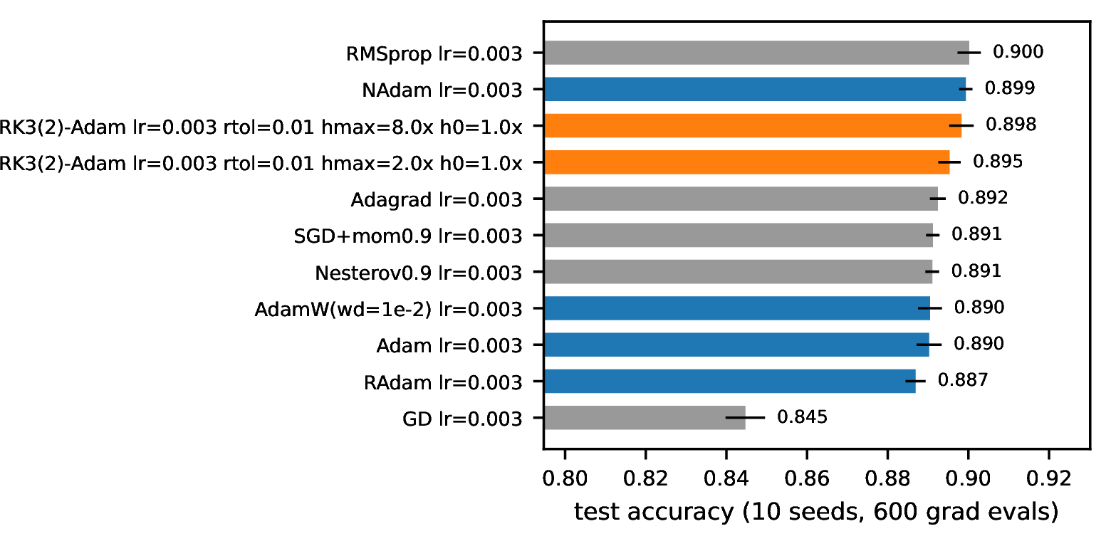
We use a deterministic full-batch gradient on a 1024-example MNIST subset—a genuine autonomous vector field, so FSAL is enabled and credited. The primary metric is final training loss (the pure “integrate gradient flow” test); GD is the Euler baseline. The baseline pool spans the standard first-order optimizers—SGD with momentum/Nesterov, Adagrad [8], RMSprop [9], Adam [7], AdamW [10], NAdam [11], and RAdam [12].

Even with a deterministic vector field, valid FSAL, and real truncation error, Adam reaches 2.4–3.4\(\times\) lower loss at equal compute (Table ¿tbl:tab:fullbatch?), and the as-designed RK3(2)-Adam is also beaten on loss by RMSprop and NAdam at \(\mathrm{lr}{=}0.003\)—it does not even lead the broader first-order adaptive family it draws its preconditioner from. Tolerance settings are again bit-identical. The comparison replicates at \(n{=}10\) seeds (Adam \(0.000117 \pm 0.000012\) vs.RK3(2)-Adam \(0.000375 \pm 0.000052\) at \(\mathrm{lr}{=}0.003\); \(\rho{=}0.01\) and \(\rho{=}0.1\) identical to the digit).

Multi-seed chase of the test-accuracy wrinkle (\(n{=}10\)). Table ¿tbl:tab:fullbatch? hints that RK3(2)-Adam generalizes better than Adam despite worse train loss. An \(n{=}10\) replication (seeds 0–9; Figure 1) confirms the effect is real and seed-consistent at \(\mathrm{lr}{=}0.003\): RK3(2)-Adam (defaults) \(89.53\%\) vs.Adam \(89.03\%\) / AdamW \(89.05\%\), winning the paired comparison on 10/10 seeds (paired \(t = 6.0\), \(+0.51 \pm 0.27\) pts); the best-loss RK configuration (\(h_{\max}{=}8\times\)) reaches \(89.83\%\), \(+0.80\) pts over Adam (\(t = 6.5\), 10/10). Two qualifiers keep this from being a headline win: (i) the effect is lr-specific—at \(\mathrm{lr}{=}0.001\) it vanishes (\(-0.08\) pts, \(t = -1.4\), RK wins 3/10 seeds); and (ii) it never clears the baseline pool—RMSprop (\(90.02\%\)) and NAdam (\(89.94\%\)) match or beat the best RK configuration at one third the per-step cost (paired \(t = -1.2\) and \(-1.3\) against \(h_{\max}{=}8\times\); \(-3.4\) and \(-5.2\) against the defaults), and Adam at \(\mathrm{lr}{=}0.01\) attains \(90.30\%\) (Table ¿tbl:tab:hmaxcontrol?). At equal gradient budget, RK gradient averaging buys a real regularization effect relative to lr-matched Adam, and nothing relative to the first-order family Adam belongs to.

5 Why the “Adaptive” Controller Is Inert↩︎

Direct instrumentation (\(\mathrm{lr}{=}0.003\), full-batch) shows \(h\) jumps from lr to \(h_{\max}= 2\,\mathrm{lr}\) on the first step and pins there for the entire run, for every tolerance tested (Figure 2a). Three compounding causes:

1. No rejection branch. The step is always accepted; \(\widehat{\mathrm{err}}\) only rescales the next \(h\). “Error control” can therefore never undo a bad step.

2. Saturation. The normalized error is far below 1 throughout training, so the growth factor saturates at its \(2.0\) cap every step and \(h\) is permanently clipped to \(h_{\max}\). The mechanism admits a precise statement:

Empirically the condition holds with wide margin: the maximum normalized error over the entire run is \(0.029\) with defaults (\(3\times\) below threshold; Figure 2b), so \(h\) is pinned for 100% of steps and the tolerance is unread in the only place it could act.

3. Inconsistent estimate. The embedded pair estimates the truncation error of the raw RK3 step \(\theta - h g_3\), but the applied update is the Adam-preconditioned \(\theta - h\, \hat{m}/\sqrt{\hat{v}}\). Moreover the FSAL stage is evaluated at the Adam point, so the “second-order solution” mixes stages of two different maps. The estimate does not measure the error of any integrator actually being run.

Consequence: the method is exactly fixed-step Adam driven by a 3-stage averaged gradient, at 3–4\(\times\) the per-step gradient cost. Under minibatch noise the same estimate is additionally swamped by gradient variance (\(\mathbb{E}\|g_3 - g_2\|\) is dominated by sampling noise, not \(h^3\) truncation error), so no choice of \(\rho\) can make it informative.

5.1 Systematic Sweep: The Diagnosis Holds Across the Hyperparameter Cube↩︎

To rule out the possibility that inertness is an artifact of one default setting, we swept the full cube \(\rho \in \{0.01, 0.1, 1.0\} \times h_{\max}\in \{2\times, 8\times\} \times h_0 \in \{0.5\times, 1\times, 2\times\}\) at both learning rates (36 RK configs + 18 baselines, 600 evals, 3 seeds each). Three findings:

1. \(\rho\) is inert across two orders of magnitude. All 12 \(\{\rho = 0.01, 0.1, 1.0\}\) triplets are bit-identical to six decimals (e.g.lr \(=0.003\), \(h_{\max}{=}8\times\): loss \(0.000109\) / \(0.000112\) / \(0.000112\)—the residual \(3{\times}10^{-6}\) gap separates \(\rho{=}0.01\) only because its first-step \(h\) differs before saturation; \(\rho{=}0.1\) and \(1.0\) agree exactly). Instrumented step counts show the step pinned at the ceiling on 98–100% of steps in every configuration. A \(100\times\) tolerance swing that changes nothing is the definition of a controller that does not control.

2. \(h_0\) is erased within a few steps. The \(h_0\) sweep produces distinct but nearly equivalent runs (lr \(=0.001\), \(h_{\max}{=}8\times\): loss \(0.000291\) / \(0.000328\) / \(0.000338\) for \(h_0 = 0.5{\times}/1{\times}/2{\times}\)) because the saturated growth factor climbs any initial step to the ceiling almost immediately (Proposition 1). The one initial condition the user can set is forgotten by the “adaptive” mechanism.

3. The only knob that matters is \(h_{\max}\)—i.e., a learning rate. Raising the ceiling \(2{\times}{\to}8{\times}\) improves loss \({\sim}4.5\times\) at lr \(=0.001\) (\(0.001488 \to 0.000328\)) and \({\sim}3\times\) at lr \(=0.003\) (\(0.000350 \to 0.000109\)). The best RK3(2)-Adam configuration in the entire 36-point cube (lr \(=0.003\), \(h_{\max}{=}8\times\): \(0.000109 \pm 0.000022\), \(89.94\%\)) statistically ties—does not beat—plain Adam at lr \(=0.003\) (\(0.000103 \pm 0.000002\)) on loss, at 3–4\(\times\) the per-step gradient cost. The effective step at that optimum is \(h \approx 8\,\mathrm{lr} = 0.024\), close to Adam’s own well-tuned regime (Table ¿tbl:tab:hmaxcontrol?: Adam lr \(=0.01\) is best overall), confirming that tuning \(h_{\max}\) is simply re-tuning the learning rate through an expensive proxy.

The sweep upgrades the diagnosis from an instrumented anecdote to an exhaustive negative: within the method as designed, there is no setting of the adaptivity hyperparameters under which the error controller influences the trajectory. All observed variation is explained by two ordinary hyperparameters—effective step size (\(\mathrm{lr} \cdot h_{\max}\) scale) and, weakly, \(h_0\)’s first-step transient.

6 Experiment 3: Repaired-Controller Ablation↩︎

Section 5.1 established that no hyperparameter setting rescues the as-designed controller; the remaining objection is that the design itself is one bug-fix away from working. We therefore repaired the controller: a true accept/reject branch (reject \(\to\) retry with smaller \(h\), no parameter update), the error measured on the actually-applied map, and \(h_{\max}= 100\,h_0\). Two variants: PureRK3(2) (raw Bogacki–Shampine step, no preconditioning—the estimate is consistent) and FixedRK3Adam (Adam-preconditioned, error on the applied update). Same full-batch protocol as Section 4.

\begin{table}[t]

Config	Train loss	Acc (%)	Rej./seed	Final \(h\)
Adam lr \(=0.001\)	\(0.000609 \pm 0.000033\)	88.57	0	—
Adam lr \(=0.003\)	\(0.000103 \pm 0.000002\)	88.92	0	—
FixedRK3Adam \(h_0{=}10^{-3}\), \(\rho{=}0.01\)	\(\mathbf{0.0000025 \pm 0.0000006}\)	88.67	9.3	0.100
FixedRK3Adam \(h_0{=}10^{-3}\), \(\rho{=}0.1\)	\(0.000005 \pm 0.000005\)	89.03	3.3	0.100
PureRK3(2) \(h_0{=}10^{-3}\) (both \(\rho\))	\(0.070635 \pm 0.000981\)	89.20	0	0.100
FixedRK3Adam \(h_0{=}0.003\), \(\rho{=}0.01\)	\(0.256485 \pm 0.279860\)	86.21	96.7	0.171
FixedRK3Adam \(h_0{=}0.003\), \(\rho{=}0.1\)	\(0.220222 \pm 0.200785\)	87.46	32.3	0.281
PureRK3(2) \(h_0{=}0.003\), \(\rho{=}0.1\)	\(0.011915 \pm 0.000085\)	89.94	0.3	0.300

\vskip

-0.1in \end{table}

With a functional controller the picture inverts on training loss (Table ¿tbl:tab:repaired?): repaired FixedRK3Adam (\(h_0{=}10^{-3}\)) reaches \(2.5\times 10^{-6}\)—\({\sim}40\times\) below the best Adam (\(1.0{\times}10^{-4}\))—and now \(\rho\) genuinely changes trajectories (rejections occur; \(\rho{=}0.01\) vs.\(0.1\) differ; Figure 2c). But the winning configurations all terminate with \(h\) pinned at the \(h_{\max}= 0.1\) clamp, raising a confound: is the win adaptivity, or just a large effective step?

\begin{table}[t]

4pt

Config	Train loss	Acc (%)
FixedStep-RK3Adam \(h{=}0.1\)	\(0.186340 \pm 0.033147\)	80.05
FixedStep-RK3Adam \(h{=}0.03\)	\(0.000639 \pm 0.000643\)	88.53
Adam lr \(=0.1\)	\(0.383101 \pm 0.115005\)	72.97
Adam lr \(=0.03\)	\(0.000115 \pm 0.000094\)	87.93
Adam lr \(=0.01\)	\(0.000068 \pm 0.000020\)	\(\mathbf{90.30}\)

\vskip

-0.1in \end{table}

The control resolves the confound in favor of adaptivity: a step fixed at the saturated \(h = 0.1\) is far worse (\(0.186\)) than the adaptive run that ends there (\(2.5\times 10^{-6}\)). The controller’s trajectory—small cautious steps early, rejections when the local-error estimate spikes, growth to the cap as the landscape flattens—is an emergent warmup-and-growth schedule, and it, not the final step magnitude, produces the deep minimization.

Three caveats bound the claim: (i) the advantage is confined to training loss—no repaired-RK configuration reaches \(90\%\) test accuracy, none matches the study-best \(90.30\%\) of Adam lr \(=0.01\) (at one third the per-step gradient cost), and Section 7 shows the shortfall is a trajectory effect, not deeper minimization; (ii) the win is fragile to the \((h_0, \rho)\) pairing—characterized below; (iii) PureRK3(2), the only variant whose error estimate is mathematically consistent, never beats Adam on loss, so the benefit comes from the controller heuristic composed with Adam, not from higher-order accuracy per se.

\begin{table}[t]

3pt

\(h_0\)	\(\rho=0.01\)	\(\rho=0.1\)
0.001	\(2.5{\times}10^{-6}\) (9.3)	\(5.3{\times}10^{-6}\) (3.3)
0.0015	\(4.9{\times}10^{-5} \pm 8.4{\times}10^{-5}\) (30.0)	\(2.9{\times}10^{-6}\) (3.7)
0.002	\(7.8{\times}10^{-2} \pm 7.6{\times}10^{-2}\) (79.3)	\(2.5{\times}10^{-6}\) (6.0)
0.0025	\(3.1{\times}10^{-2} \pm 3.2{\times}10^{-2}\) (81.0)	\(\mathbf{3.8{\times}10^{-7}}\) (6.7)
0.003	\(2.6{\times}10^{-1} \pm 2.8{\times}10^{-1}\) (96.7)	\(2.2{\times}10^{-1} \pm 2.0{\times}10^{-1}\) (32.3)

\vskip

-0.1in \end{table}

The fragility boundary. A five-point \(h_0\) grid (Table ¿tbl:tab:fragility?, Figure 3) shows the instability tracks the pairing of \(h_0\) with \(\rho\), not \(h_0\) alone—and, counterintuitively, the tighter tolerance is the fragile one. \(\rho{=}0.01\) begins degrading at \(h_0 = 0.0015\) and is broken by \(0.002\); \(\rho{=}0.1\) is stable—indeed deepest (\(3.8\times 10^{-7}\), the lowest loss in the study)—through \(0.0025\). The mechanism is visible in the rejection column: stable runs reject 3–10 steps/seed, broken runs 30–97; a tight tolerance turns large-\(h_0\) transients into reject-retry thrashing that consumes the eval budget, while the looser tolerance rides through them. The rejection rate is thus a leading indicator of the instability, reinforcing the reporting standard of Section 9. Across these configurations, deeper minima co-occur with lower test accuracy (\(89.03\%\) at \(h_0{=}0.001 \to 86.95\%\) at \(h_0{=}0.0025\))—tempting to read as over-minimization overfitting, but it confounds minimization depth with the controller trajectory that reaches it. Section 7 disentangles the two with a pre-registered test and finds the depth reading is wrong.

7 Experiment 4: The Generalization Deficit Is Trajectory-Driven, Not Tempering↩︎

Section 6 leaves a puzzle: the repaired controller drives training loss \({\sim}40\times\) below Adam yet generalizes worse than a moderately-tuned baseline. A fashionable explanation is tempering. An optimizer minimizing a loss \(L\) is, in the Langevin view, sampling the Gibbs density \(p(\theta) \propto \exp(-L/T)\) at temperature \(T \to 0\); deep minimization is cold sampling, and the cold-posterior effect [6] establishes that generalization can be non-monotone in \(T\) with an interior optimum \(T^* > 0\). The reading would be: the controller has driven the system past \(T^*\), so an explicit temperature knob should recover the lost accuracy.

We tested this directly, grounding the controller’s implicit tempering as an explicit temperature via preconditioned Stochastic Gradient Langevin Dynamics (pSGLD; [13]), the SG-MCMC kernel closest to our Adam-preconditioned update: \[\theta \leftarrow \theta - \mathrm{lr}\, M g + \sqrt{2\,\mathrm{lr}\, T\, M}\, \eta, \quad \eta \sim \mathcal{N}(0, I),\] with \(M = \mathrm{diag}(1/(\sqrt{\hat{v}} + \epsilon))\) the RMSprop preconditioner (\(T = 0\) recovers a deterministic minimizer; the divergence-correction term is dropped, per [13]). Because our controller carries Adam momentum, its exact SG-MCMC analogue is the underdamped SGHMC [14]; pSGLD is the overdamped simplification that suffices to move the temperature knob. Two predictions were pre-registered in code before running: H1 (tempering supported)—test accuracy is non-monotone in \(T\) with an interior optimum, and the within-run accuracy trajectory at \(T = 0\) peaks then declines; H0 (refuted)—\(T = 0\) is best and no overfitting peak exists.

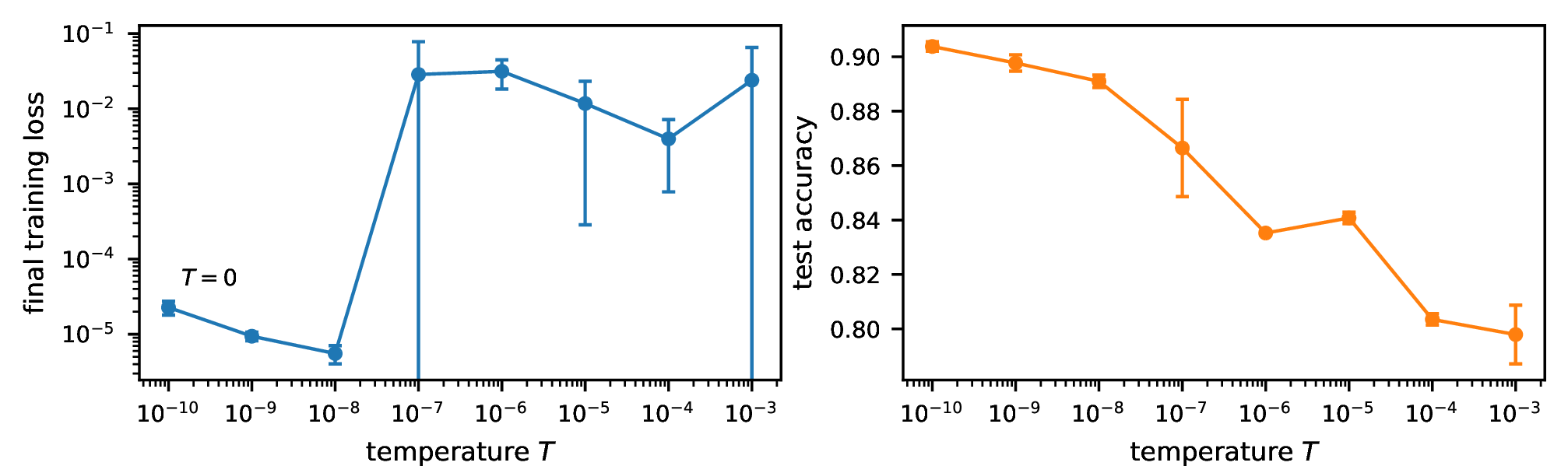
Test 1—does pure minimization overfit? No. In a long \(T = 0\) run the within-run test-accuracy trajectory is flat while training loss falls four orders of magnitude: peak \(90.77\%\) at eval 200 (loss \(1.6\times 10^{-3}\)), \(90.58\%\) at eval 6000 (loss \(9\times 10^{-7}\))—a \(0.19\)-pt change. Across 5 seeds the deep-minimization endpoint (loss \(1.12\times 10^{-6}\)) tests \(\mathbf{90.37 \pm 0.24\%}\), statistically identical to its shallow-minimization accuracy. Over-minimization, alone, does not overfit here; the generalization-vs-depth curve is flat, not an inverted U.

Test 2—does temperature help? No. \(T = 0\) gives the best test accuracy and is the global optimum of the sweep—no \(T > 0\) comes within \(0.6\) pt (Figure 4)—so the automated, pre-registered verdict returns H0. For \(T \le 10^{-8}\) the injected noise is negligible; for \(T \ge 10^{-7}\) the noise floor dominates and accuracy collapses (\(90.38\%\) at \(T{=}0\) down to \(79.79\%\) at \(T{=}10^{-3}\)). The preconditioner-free SGLD arm [15] agrees—no temperature meaningfully improves accuracy—but is a weak testbed, since unpreconditioned descent barely minimizes, plateauing at loss \(6.9\times 10^{-2}\). Both tests return H0: the tempering reinterpretation is not supported.

What the negative reveals. Ruling out depth and temperature isolates the real mechanism. At matched training-loss depth the trajectories diverge sharply in generalization: a plain RMSprop minimizer (pSGLD, \(T = 0\)) reaches loss \(1.1\times 10^{-6}\) at \(\mathbf{90.37\%}\) and steady Adam (\(\mathrm{lr}{=}0.01\)) \(6.8\times 10^{-5}\) at \(90.30\%\), yet the repaired FixedRK3Adam reaches the same \({\sim}10^{-6}\) depth at only \(88.7\)–\(89.0\%\), and its deepest configuration (\(3.8\times 10^{-7}\)) at \(86.95\%\)—1.3 to 3.4 points worse than a steady first-order minimizer at equal or greater depth. Depth is generalization-neutral; temperature only hurts; so the deficit is a property of which minimum the trajectory selects. The controller’s emergent warmup–growth–reject schedule evidently lands in a worse-generalizing region than the smooth descent of a fixed-step method (we do not measure curvature, so we stop short of asserting sharper minima). The right frame is implicit-bias-of-optimization, not tempering; and it is one more way the RK machinery changes the path without improving the destination—the paper’s thesis, sharpened on the very axis where the repaired controller had looked like it might matter.

8 Related Work↩︎

Optimizers as ODE discretizations. The continuous-time view was crystallized by [2], who derived a second-order ODE as the continuum limit of Nesterov’s accelerated gradient method; a large literature has since studied optimization dynamics through Lyapunov analysis of such flows. The direct precedent for our study is [3], showing that explicit RK integration of the gradient/Nesterov flow attains accelerated convergence-rate guarantees for smooth, sufficiently regular convex objectives. Crucially, those rates are stated per iteration; each RK iteration of an \(s\)-stage scheme costs \(s\) gradient evaluations, and the per-gradient-evaluation accounting we enforce is exactly the regime where the theoretical advantage must pay rent. França and collaborators’ work on conformal-symplectic and dissipative-Hamiltonian integrators [16], [17] makes a related structural argument—that preserving geometric properties of the flow, rather than raw order of accuracy, is what matters—consonant with our finding that higher-order accuracy per se (PureRK3(2), the only consistent integrator we test) never beats Adam on loss.

RK-flavored practical optimizers. Several recent proposals inject higher-order integration machinery into Adam-style updates. IMEX/semi-implicit schemes treat the preconditioner implicitly and the gradient explicitly: [18] show that classical Adam is a first-order IMEX-Euler discretization and propose higher-order IMEX variants. A related line drives adaptive moments with neural-ODE machinery [19]. Our design is deliberately representative of this family: Bogacki–Shampine 3(2) stages, FSAL reuse, embedded-pair step control, composed with Adam preconditioning. Two accounting conventions recur in this literature and flatter the RK side: (i) comparisons per optimizer step rather than per gradient evaluation, hiding the 3–4\(\times\) stage cost; and (ii) FSAL credited under minibatch sampling, where the cached stage belongs to a different (previous batch’s) vector field and the reuse is not mathematically valid. Our protocol disallows both, and under it the headline advantages shrink or invert.

Adaptive step-size control. Embedded-pair local-error control [4], [5], [20] is standard in ODE solvers, but its transplantation into optimizers is usually decorative: as we diagnose in Section 5, without a rejection branch, and with the error measured on a map that is never actually applied, the controller saturates and the method degenerates to fixed-step Adam with an averaged gradient. We are not aware of prior work that (a) instruments whether the controller in an RK-optimizer ever alters a step, or (b) repairs it and re-runs the comparison; Section 6 does both. The emergent warmup-and-growth schedule we observe connects to the literature on learning-rate warmup—the repaired controller effectively discovers a warmup schedule from local-error feedback.

Optimization as sampling. Casting an optimizer as a Markov chain that samples \(\exp(-L/T)\) connects our repaired controller—itself an accept/reject kernel—to stochastic-gradient MCMC: SGLD [15], its preconditioned form pSGLD [13], and the momentum variant SGHMC [14], whose friction term is the sampling-world analogue of our finding that minibatch noise corrupts the embedded error estimate. We use this lens actively in Section 7, grounding the controller’s implicit tempering as an explicit temperature to test—and refute—a cold-posterior [6] reading of its generalization deficit. The lens also explains why higher-order RK is a poor fit for sampling: the one setting where careful trajectory integration is genuinely load-bearing for a Markov chain—Hamiltonian Monte Carlo [21]—deliberately uses symplectic leapfrog integration rather than generic RK, because the Metropolis correction needs reversibility and volume preservation that explicit RK lacks; and the HMC-integrator literature [22] selects schemes by energy error per force evaluation—the same per-gradient accounting we enforce—concluding that structure preservation, not raw order, is what pays.

Positioning. Relative to the acceleration-theory line, we supply the missing per-eval empirical accounting in the non-convex setting; relative to the practical RK-optimizer line, we supply the controller instrumentation, the repaired-controller ablation, and the fixed-step control that isolates adaptivity (not order, not step magnitude) as the operative mechanism.

9 Discussion↩︎

Training is not trajectory-tracking. The optimization objective rewards reaching low loss, not shadowing the continuous gradient-flow solution; higher-order accuracy buys fidelity to a trajectory nobody needs, at a price (3–4\(\times\) evals/step) that compute-matched evaluation makes visible. Once the budget is denominated in gradient evaluations, a method must convert its extra per-step accuracy into a \(>3\times\) improvement in per-step progress just to tie—a bar none of the as-published variants clears in our experiments. Prior RK-optimizer results reporting per-iteration or wall-clock-favorable comparisons should be re-read with per-gradient-eval accounting.

“Adaptive” must be verified, not assumed. The most transferable finding is methodological: the error controller in our as-designed method—and, we suspect, in relatives that share its structure—was doing literally nothing (bit-identical trajectories across tolerances; \(h\) pinned at its cap from step one). None of the standard reporting practices in this literature would have caught this: train curves, final accuracies, and even tolerance “sweeps” all look like plausible experiments while the adaptive machinery is inert. We suggest a minimal reporting standard for adaptive-step optimizers: (i) the distribution of accepted \(h\) over training—in particular the fraction of steps pinned at the ceiling (98–100% in every cell of our sweep), (ii) the rejection rate, and (iii) a demonstration that at least two controller settings produce non-bit-identical trajectories. Point (iii) needs teeth: in our sweep, tolerances spanning two orders of magnitude were bit-identical to six decimals, so a narrow two-point “sweep” that happens to straddle no behavioral boundary proves nothing—the \(h\) distribution in (i) is the check that cannot be faked.

What the repaired controller tells us. Two positive signals survive our protocol. First, the repaired controller shows that embedded-pair adaptivity composed with Adam yields an emergent warmup-and-growth step schedule that minimizes training loss far below tuned Adam at equal budget (\({\sim}40\times\))—a genuine mechanism, isolated from the large-step confound by a fixed-step control, and from the depth and tempering confounds by Section 7. Notably, the controller rediscovers learning-rate warmup from local-error feedback alone, suggesting that hand-designed warmup schedules may be approximating an error-control policy; making that correspondence precise is an attractive theory question. Second, the \(n{=}10\) multi-seed chase (Section 4) upgrades the implicit-regularization observation from anecdote to finding: RK3(2)-Adam beats lr-matched Adam and AdamW on test accuracy on 10/10 seeds despite \({\sim}3\times\) worse train loss—consistent with gradient averaging and integration error acting as implicit regularization. The catch is redundancy: RMSprop, NAdam, and lr-tuned Adam reach the same or better accuracy with no RK machinery, so the effect is real but not competitive—it repairs a deficiency of fixed-lr Adam rather than advancing the frontier.

Where the train-loss win could matter. A \({\sim}40\times\) train-loss advantage with no test-accuracy gain is not useless: deterministic small-data regimes where optimization is the objective—physics-informed losses, implicit-layer and equilibrium-model inner solves, distillation to near-zero loss, overfitting benchmarks—are settings where full-batch gradients are genuine and FSAL is valid. That is the honest market for this mechanism. Any salvaged positive claim must be about one of these, not about faster optimization of the deployed metric: on test accuracy, modestly tuned Adam (\(\mathrm{lr}{=}0.01\), \(90.30\%\)) beats every RK variant at one third the per-step cost.

9.1 Limitations↩︎

(1) Scale and scope: all results are on MNIST (full set for stochastic, 1024-example subset for full-batch) with a single 784–128–10 MLP; the compute-matched methodology transfers, but the empirical rankings may not. (2) Statistics: \(n{=}3\) seeds per cell for the main sweeps; headline gaps are far outside seed noise, and the secondary test-accuracy observation was chased at \(n{=}10\) with paired statistics; the repaired-controller tables remain \(n{=}3\). (3) One design point: our inertness diagnosis is structural and should apply to relatives sharing the no-reject/raw-map-error design, but we did not re-implement published variants, and IMEX/implicit schemes have a different failure surface we do not probe. (4) Baseline tuning asymmetry: Adam received a modest lr grid; the RK variants an equally modest \(h_0/\rho\) grid; the repaired method’s documented \(h_0\) fragility means a finer sweep could move results in either direction. (5) Repaired-controller generality: the \({\sim}40\times\) result is full-batch, deterministic, and fragile to \(h_0\); we have no evidence it survives minibatch noise, where the error estimate is variance-dominated by our own diagnosis—repairing the controller does not repair the estimator. (6) Compute-matching granularity: we count gradient evaluations and ignore per-step optimizer overhead, which slightly favors the RK methods. (7) The implicit-regularization observation is post hoc, emerging from inspection of result tables, and is presented accordingly. (8) Minimum-selection mechanism is identified only by exclusion: we do not instrument loss-surface curvature at the selected minima, so the implicit-bias mechanism is named, not measured.

10 Conclusion↩︎

We set out to test a clean and appealing idea—that better ODE integrators make better optimizers—and found the honest answer to be mostly no, for an instructive reason. Under a protocol that denominates budget in gradient evaluations, a representative Bogacki–Shampine 3(2) RK–Adam loses to plain Adam on training loss in both stochastic and full-batch settings, and its “adaptive” step controller turns out to be inert: the step size saturates on the first iteration and the tolerance parameter has no effect on the trajectory at all. Diagnosing the inertness and repairing it reverses the full-batch training-loss result by \({\sim}40\times\), but a fixed-step control localizes the benefit to adaptivity—an emergent warmup-and-growth schedule—rather than to higher-order accuracy, and the benefit does not reach test accuracy. A pre-registered temperature sweep rules out the two off-the-shelf explanations for that gap, pinning the generalization shortfall on which minimum the controller’s trajectory selects rather than on how deep it minimizes.

The durable contributions are therefore methodological rather than a new optimizer: (1) a per-gradient-evaluation accounting discipline, with FSAL credited only where it is mathematically valid, that changes the sign of the comparison; (2) the observation that adaptive-step optimizers can ship a controller that never controls anything, together with a minimal reporting standard that would expose it; and (3) a seed-consistent implicit-regularization effect of RK gradient averaging that nonetheless never clears the tuned first-order baseline pool—a compact illustration of why optimizer claims need baseline pools rather than a single anchor. For anyone continuing the RK-optimizer program, the useful frontiers are the ones where the training-loss mechanism we isolated actually pays: deterministic, small-data, optimization-is-the-objective regimes; a variance-corrected error estimator that could make the controller meaningful under minibatch noise; and a precise account of the emergent warmup schedule as an implicit error-control policy. We release all code, logs, and results to make each of these directly checkable.

Reproducibility Statement↩︎

All experiments run on CPU with deterministic seeding. Code, result JSONs, and logs are released with the paper: RK4Optimizer.py (optimizer implementations), mnist_experiment.py (Experiment 1), fullbatch_experiment.py (Experiment 2 and the hyperparameter cube), fixed_controller_experiment.py (Experiment 3), hmax_control_experiment.py (the fixed-step control), and temperature_sweep_experiment.py (Experiment 4, with the pre-registered H1/H0 criteria and automated verdict in the module docstring). Figures are regenerated by make_trajectory_data.py and make_figures.py.

References↩︎