Introduction↩︎

Machine-learning force fields (MLFFs) are widely used for atomistic simulation at near density-functional-theory (DFT) accuracy and classical-molecular-dynamics throughput[1]–[3]. Their accuracy and reliability depend strongly on the training data: an MLFF is accurate on configurations close to its training distribution, but its predictions are usually weakly constrained on configurations outside it[4]–[6]. Two training paradigms now coexist in the field. The traditional train-from-scratch (TFS) approach trains an MLFF on a system-specific dataset, typically a few hundred to a few thousand DFT-labelled configurations of the target chemistry[6], [7]. The more recent fine-tuning (FT) approach[8]–[13] starts from a foundation MLFF pretrained on a large and chemically diverse structure collection and adapts it to a target system using a much smaller fine-tuning dataset. The data-quality and out-of-distribution issues that affect MLFFs in general persist in the FT setting and can be more severe: a foundation has seen such a broad swath of chemistries that it tends to return confident-looking predictions even far from the target system, so when the model is in fact extrapolating the failure is easy to miss[6], [12], [14].

A trained MLFF needs to do two things well, regardless of training paradigm. The first is the conventional training criterion: the energy and force errors on a held-out test set are sufficiently small, indicating that the network parameters are well fit to the labelled data[15]. The second, and arguably more important, is that once deployed in molecular dynamics the model is both stable, in the sense that the trajectory does not crash or develop numerical instability, and reliable, in the sense that the configurations sampled and the observables predicted are consistent with what an MD run at the labelling level of theory would produce[6], [14], [16], [17]. The training and test sets are pre-constructed and represent only a snapshot of the relevant chemical space; once deployed in MD the model is free to explore configurations that may not appear in either set, and where it must extrapolate, the predicted potential energy surface is not constrained to be accurate[4]–[6]. Thus, even an MLFF with low test-set MSE can produce unstable or unphysical MD when thermal fluctuations sample configurations outside the training distribution[14], [16]. The generalisation gap between test-set error and downstream-task reliability is particularly acute in MLFFs, because the configurational space of a chemical system is vastly larger than any practical labelled dataset and MD actively probes that space at every timestep.

What ultimately matters is the dataset itself. At a fixed budget of \(N\) labelled configurations, a dataset that spreads its frames across the relevant region of configuration space generalises better in MD than one that concentrates the same number of frames in a narrow region. The central question for MLFF data generation is therefore not how much data to generate but which data[6], [7], [18]. A principal approach for assembling such a dataset is active learning (AL)[7], [19]–[23], an iterative procedure in which an uncertainty quantification (UQ) signal computed by the model itself drives configuration selection. A standard active-learning workflow, implemented in tools such as DPGEN[24] and AI\(^2\)-kit[25] as well as in many in-house pipelines, alternates exploratory MD with the current model, uncertainty-ranked frame selection, DFT labelling, and retraining, until the model is judged converged.

The most common UQ signal in MLFF active learning is the model committee[19]–[22], in which several MLFFs are trained from independent random initialisations on the same data and the spread of their predictions on a query configuration is taken as the uncertainty estimate[21], [26]. The model committee is conceptually simple and transfers across MLFF architectures, but it has a clear cost: every additional committee member is a full extra training run. The overhead grows with model size and with training-dataset size, and becomes severe at foundation MLFF scale: training, for example, four foundation copies merely to obtain a UQ signal on a target system is rarely a practical operating point. Several alternative UQ signals have been proposed in recent work on foundation MLFFs, including dedicated confidence-head outputs trained alongside the main potential[27], heterogeneous ensembles that aggregate predictions across diverse pretrained foundations[28], quantile-regression heads that estimate prediction intervals directly[29], and environment-dependent post-hoc calibration that improves uncertainty–error correlation and high-error-configuration detection[30]. Among these, the last-layer-projection regression (LLPR) framework[31] is particularly attractive: it uses the model’s own last-layer features together with the covariance over the training set to estimate per-configuration uncertainty in a single forward pass. LLPR was first applied to MLFFs in the train-from-scratch setting on QM9 and bulk water[31]; recent flexible-calibration work has also used LLPR as a baseline UQ signal for MACE-MP-0 and demonstrated high-error detection and active fine-tuning[30]. What remains unestablished is a unified LLPR workflow that spans both train-from-scratch and foundation fine-tuning while combining pre-labelling pathology detection, iterative data selection, and self-termination in absolute error units.

In this work we implement and integrate LLPR-based UQ signals into active-learning and fine-tuning workflows, and demonstrate that, with appropriate design choices, an LLPR-driven picker reaches full-data accuracy with substantially fewer labels than both random selection and the model committee, in both train-from-scratch and fine-tuning settings. We also find that the LLPR-based uncertainty serves as an early indicator when a foundation model is operationally bad, and is most valuable in the more dangerous case we demonstrate here, where the foundation MD runs stably yet samples structurally wrong configurations — a failure mode that conventional stability diagnostics cannot detect. We demonstrate the workflow across three systems: train-from-scratch active learning on an open water/ice dataset[32], [33], one-shot fine-tuning of MACE-MP-0 on the same water/ice target, and iterative active fine-tuning of an OMAT-small foundation[9] on a 21 molal LiTFSI water-in-salt electrolyte for which the initial foundation MD is stable but structurally hallucinated. The resulting workflow provides a light yet accurate UQ signal that supports self-terminating active learning without an external oracle and detects deployment-MD hallucinations that conventional validation diagnostics miss, achieving full-data accuracy with substantially fewer DFT labels in both train-from-scratch and foundation fine-tuning regimes.

Results↩︎

LLPR-based uncertainty quantification in MLFFs↩︎

To validate that LLPR gives quantitatively calibrated uncertainty for an MLFF and to assess its effectiveness as a picker for active learning, we evaluate it on a DeePMD model of liquid water trained on 50 frames of 64-water cells. The held-out evaluation pool comprises 2027 frames in total: 965 in-distribution 64-water configurations, 1022 out-of-distribution 63-water configurations, and 40 out-of-distribution 128-water configurations, with the OOD subsets deliberately chosen as cell-size shifts of the training-set chemistry. The water configurations are drawn from the dataset of Fu et al.[34], and full details of the model and the data partition are in Methods. From the model’s last-layer features and the covariance over its training set we compute two LLPR uncertainty signals: a per-frame energy LLPR \(\sigma^2_E\) that scores the uncertainty of the model’s predicted total energy of a frame, and a top-5 force LLPR \(\sigma^2_F\) that scores its local force uncertainty as the per-frame mean of the five largest per-atom uncertainties (for details see Methods); averaging the five most-uncertain atoms rather than picking the single most-uncertain one suppresses the noise of the single-forward statistic. \(\sigma^2_E\) is therefore a global per-frame signal, \(\sigma^2_F\) a localised per-atom signal aggregated to a frame. For comparison we also compute committee disagreement: the spread of energy and force predictions across four MLFFs trained from independent random seeds, the standard MLFF active-learning UQ baseline.

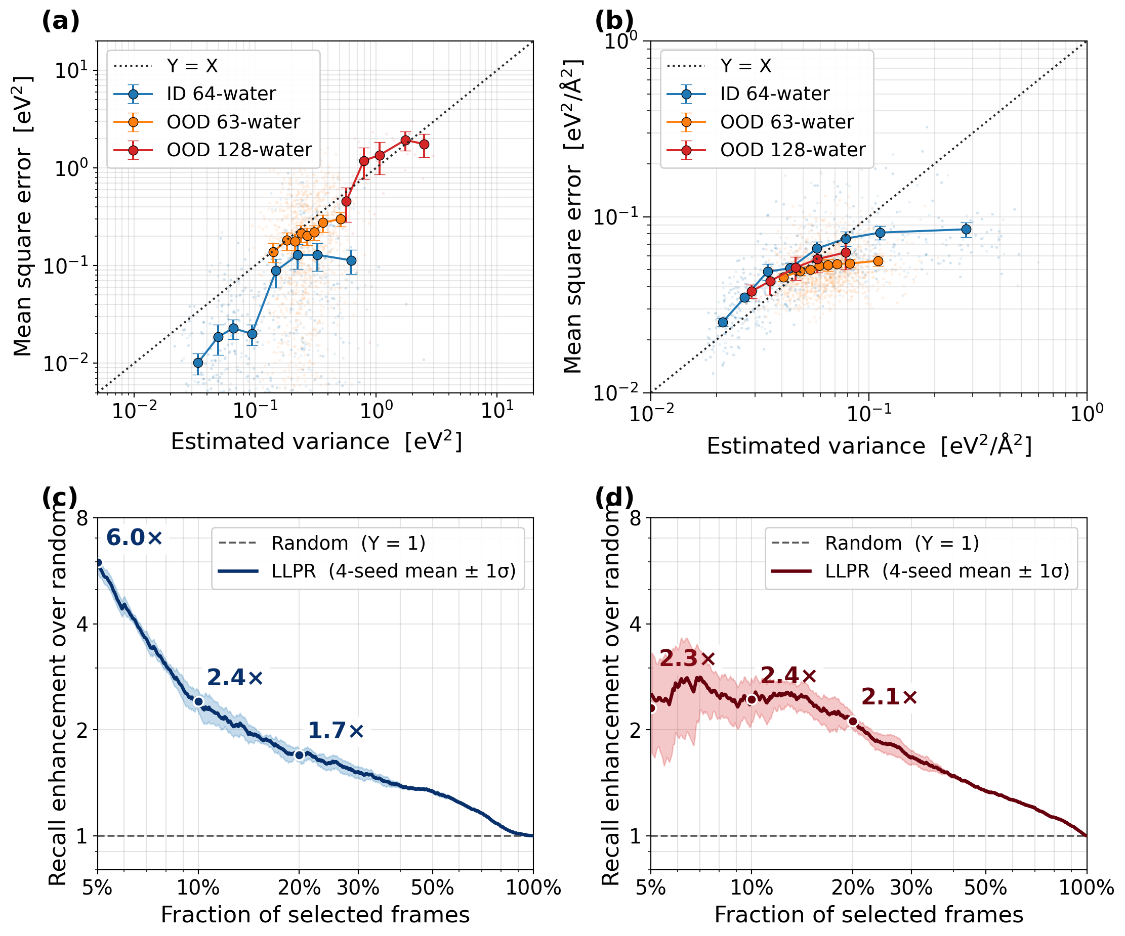
Both energy LLPR (\(\sigma^2_E\)) and force LLPR (\(\sigma^2_F\)) correlate strongly with the actual prediction error and provide quantitative uncertainty estimates. Figure 1a and Figure 1b plot the bin-mean predicted \(\sigma^2\) against the bin-mean observed squared error for the energy and force signals respectively, in equal-count bins of the 2027-frame pool with the \(y = x\) diagonal as the reference for exact agreement. A frame with high LLPR \(\sigma^2\) shows a correspondingly larger actual error on average. The LLPR signals can therefore be used as quantitative uncertainty estimates and not merely as a ranking statistic.

Resolving the bin-mean curves by group reveals a clear ID/OOD contrast in energy LLPR but not in force LLPR. In Figure 1a, the in-distribution 64-water frames give the lowest \(\sigma^2_E\), the 63-water OOD frames give moderately higher values, and the 128-water OOD frames give the highest \(\sigma^2_E\). This ordering is expected: the model was trained on 64-water cells, so 63- and 128-water cells are both extrapolations, but 128-water is the more extreme one in terms of total system size. In Figure 1b, by contrast, the per-atom force-uncertainty distributions of the three groups overlap rather than separate. Force LLPR is a strictly local signal, so it does not respond to cell-size shifts as long as the local water environment around each atom looks the same across 64-, 63-, and 128-water cells at roughly the same density. Energy LLPR aggregates over all atoms of a frame and therefore does respond to total-system-size differences that leave the local environments intact.

To further test whether these signals translate into effective pickers for active learning, we measure their retrieval performance, defined as how often a top-K pick by LLPR-\(\sigma^2\) coincides with the top-K worst-error frames (i.e., frames with the largest true prediction error), and compare it against random sampling as the no-signal baseline. Figure 1c and Figure 1d plot the enrichment factor for energy LLPR and force LLPR respectively, defined as the fraction of worst-K frames recovered by LLPR divided by the fraction a random picker recovers at the same budget ratio K/N (K = number of picks, N = size of the pool). For energy-LLPR retrieval (Figure 1c), LLPR delivers a 6.0 times enrichment over random at K/N = 5%, 2.4 times at K/N = 10%, and 1.7 times at K/N = 20%; the enrichment then declines smoothly to 1 as K/N approaches 100%, where random sampling alone hits every worst frame by querying the whole pool. For force-LLPR retrieval (Figure 1d), the enrichment is more modest at the smallest budget (2.3 times at K/N = 5%) but plateaus across the small-K regime (2.5 times at K/N = 10%, 2.1 times at K/N = 20%), reflecting the noisier per-atom resolution of the force signal compared with the cleaner per-frame energy. The cross-seed error bands in both panels are tight across the entire K/N range, indicating that the LLPR signal has a high signal-to-noise ratio and that picks made with a single trained model can be trusted as confidently as those that would normally require a multi-seed committee.

Validating LLPR in an end-to-end active-learning workflow↩︎

The validation above showed that LLPR’s energy and force uncertainties both agree quantitatively with the true prediction error and are effective as pickers. We now test whether this picker performance transfers to an end-to-end active-learning workflow that produces a train-from-scratch MLFF, and how the resulting models compare against a from-scratch full-data ceiling.

To make the comparison fair we designed a controlled active-learning experiment on the water/ice dataset from Morawietz et al.[32], [33], which contains 7241 RPBE-D3 configurations of liquid water and ice polymorphs ranging from low-density liquid to compressed ice. Training an MLFF on this dataset is substantially more challenging than training one for liquid water alone, because the model must simultaneously capture a disordered liquid phase and several distinct crystalline phases with remarkably different densities, coordination environments, and hydrogen-bond topologies, all within a single set of network parameters. A controlled design holds everything except the UQ method constant: each strategy draws from the same pre-labelled candidate pool in each round, the cumulative picks are used to retrain the model under a fixed recipe, and every model is evaluated on the same held-out test set. Two reference baselines are essential to this comparison: random sampling, against which any improvement tells us that the UQ signal is what helps, not merely that the dataset is growing larger; and a from-scratch full-data ceiling, defined as a same-architecture MLFF trained on the entire candidate pool under the same recipe.

The bootstrap model is a DeePMD potential trained on the liquid-water subsystem of the Morawietz dataset. A multi-phase test set of 990 configurations is held out for evaluation: 500 additional liquid frames from the same subsystem plus 490 ice frames spanning the four ice-phase groups (ice_low, ice_mid, ice_XV and ice_VIII, as defined in Methods). The active-learning candidate pool from which each strategy picks consists of 1140 ice frames, namely the remaining 70% of those four ice-phase groups not held out for testing; every ice configuration in this pool is out-of-distribution for the bootstrap model by construction.

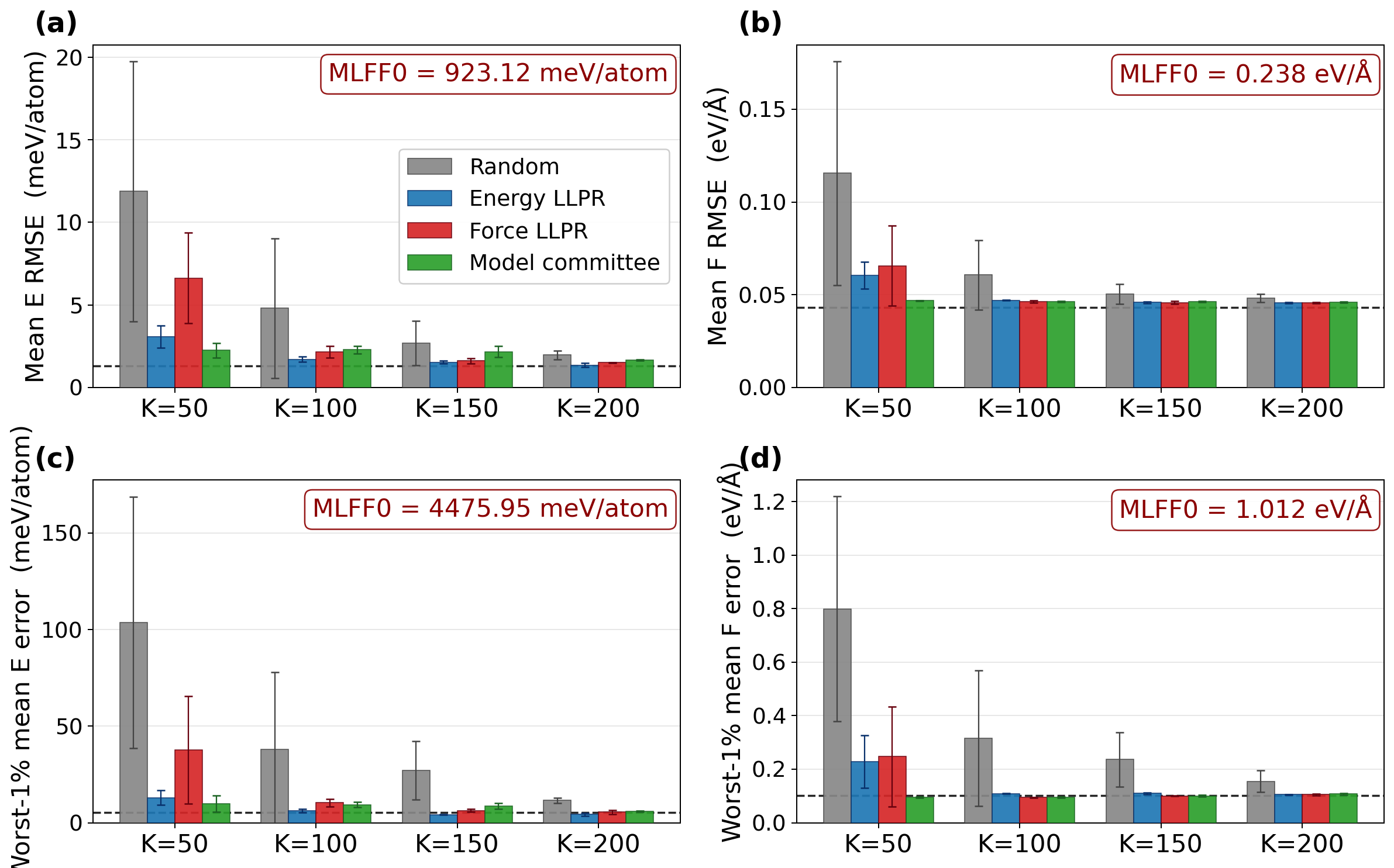
The bootstrap model is reasonably accurate on the liquid partition of the test set, with a mean energy RMSE of about 1.4 meV/atom and a mean force RMSE of about 0.057 eV/Å (see SI). Its worst-1% mean energy and force errors, however, are approximately 4476 meV/atom and 1.01 eV/Å respectively (Figures 2c, 2d), showing that the bootstrap is severely inaccurate on the hardest test frames. The from-scratch full-data ceiling is a model trained under the same recipe on all the small-cell training data available; this ceiling reaches a worst-1% mean energy error of 5.4 meV/atom and a worst-1% mean force error of 0.102 eV/Å, roughly three orders of magnitude better on energy and one order of magnitude better on force than the bootstrap. Per-subsystem errors of the bootstrap and the full-data ceiling are tabulated in Table S1.

We then test the two LLPR uncertainty signals as picking strategies in this workflow, together with random sampling and the model committee as reference baselines. Energy LLPR and force LLPR are the two signals defined in the previous subsection; the model committee here is the per-frame mean of the five largest per-atom force-spread values across a four-member committee of independently-trained MLFFs. For each strategy and each label count K, we train a single model on a 200-frame liquid anchor (a random subset of the bootstrap’s liquid-water training set) together with the K frames picked by that strategy from the candidate pool. Every retrained model is warm-started from the bootstrap weights and trained under the same annealed schedule, so the comparison between strategies isolates which K ice picks were added. We retrain at four label counts, K = 50, 100, 150 and 200, with three independent retraining seeds at each K. Within the K picks of each strategy, frames are diversified by SOAP-FPS[35] on top of the uncertainty score to avoid selecting nearly-identical frames; the detailed retraining setup is given in Methods.

Figures 2a and 2b show the test-set RMSE on energy and on force respectively for the four picker strategies across the K-sweep. At the smallest label count K = 50, the three uncertainty-driven pickers already largely outperform random sampling on the bulk metrics. On mean E (Figure 2a), the model committee is the strongest of the four pickers at about 2.2 meV/atom, followed by energy LLPR at about 3.1 and force LLPR at about 6.6, while random sampling lags behind at about 11.9 meV/atom. On mean F (Figure 2b) the same ordering holds, with committee at about 0.05 eV/Å, energy LLPR at about 0.06 eV/Å, force LLPR at about 0.07 eV/Å, and random at about 0.12 eV/Å. At K = 100, all three uncertainty-driven pickers remain above random and the LLPR pickers catch up with committee: energy LLPR reaches a mean E of about 1.7 meV/atom against committee’s 2.3, both approaching the full-data ceiling of 1.30 meV/atom; on mean F all three uncertainty-driven pickers are within 9% of the 0.043 eV/Å ceiling, while random sits at about 0.06 eV/Å. From K = 150 to K = 200 the uncertainty-driven pickers plateau close to the ceiling, while random keeps improving with K but does not fully close the gap.

This contrast indicates that the uncertainty-driven strategies efficiently cover the structurally informative regions of the candidate pool by about K = 100, whereas random sampling needs more frames to do the same coverage by chance. At medium-to-large K the LLPR pickers are also slightly ahead of the model committee on the mean metrics, indicating that the LLPR uncertainty signal carries comparable or stronger discriminative information than the committee spread for picking, and at a substantially lower training cost, since building a model committee requires training multiple independent models whereas LLPR only requires one. Notably, at K = 100 the LLPR-driven workflow already reaches a mean test E of about 1.7 meV/atom and a mean test F of about 0.047 eV/Å on a training set of only 300 frames (the 200-frame liquid anchor plus 100 picks), within 31% of the full-data ceiling on energy and within 9% of the full-data ceiling on force; this confirms that near full-data accuracy can be reached with substantially fewer labels when those labels are selected by an informative UQ signal.

Figures 2c and 2d show the worst-1% mean test E and worst-1% mean test F respectively, i.e.the mean error over the top-1% of frames with the largest per-frame error. This metric is more discriminating than the bulk mean E and mean F because it isolates exactly the rare hard frames where the model breaks down. The contrasts between strategies are accordingly much sharper. At K = 50, random reaches a worst-1% mean E of about 103.7 meV/atom and a worst-1% mean F of about 0.80 eV/Å, whereas the model committee reaches about 9.8 meV/atom and 0.095 eV/Å, an order of magnitude lower on energy and a factor of eight lower on force. The two LLPR pickers are intermediate at K = 50 and reach committee-level worst-1% performance by K = 100. All three uncertainty-driven pickers converge to within a factor of two of the full-data ceiling (5.4 meV/atom on worst-1% mean E, 0.102 eV/Å on worst-1% mean F) by K = 100, while random sampling is still about 7 times above the ceiling on energy and 3 times above on force at the same K.

A further practical benefit of the uncertainty-driven pickers is reproducibility: their cross-seed standard deviations on the worst-1% mean are much smaller than random sampling’s at every K, as the uncertainty ordering deterministically prioritises the same high-leverage frames regardless of seed (for example, at K = 100 the cross-seed standard deviation on worst-1% mean E is about 1 for the LLPR pickers and the committee, against about 40 for random). This level of determinism matters in practical deployment, and the LLPR pickers achieve committee-level determinism with only a single trained model.

Extending the workflow to foundation MLFF fine-tuning↩︎

The from-scratch case above demonstrated the LLPR-based data-selection effect on a model trained from random initialisation. In practice, deploying an MLFF to a new system is increasingly done by fine-tuning a foundation MLFF[9]–[12]. We next investigate whether the same data-selection effect extends to the fine-tuning regime. We retain the Morawietz water/ice candidate pool used in the previous regime and replace the from-scratch DeePMD bootstrap with the MACE-MP-0 foundation[10]. MACE-MP-0 small is used as the primary foundation, and MACE-MP-0 medium is included for a model-size comparison. The fine-tuning recipe uses the multihead approach; full hyperparameters (replay buffer, loss weights, learning rate, etc.) are in Methods. As in the from-scratch case, K denotes the cumulative number of DFT-labelled frames acquired by the active-learning workflow. We sweep K from 50 up to 200 in steps of 50 with three retraining seeds per cell. A model-committee baseline is not presented in this regime: constructing one would require multiple independent foundation fine-tuning runs, which is computationally impractical.

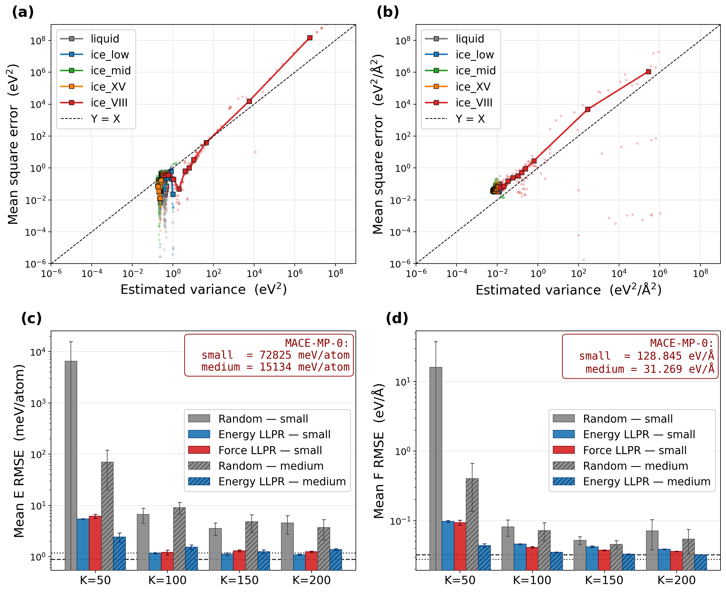
Figure 3a–b show the LLPR-based uncertainty estimation on MACE-MP-0 small. The energy and top-5 force uncertainties are evaluated against their ground-truth squared errors on the candidate pool combined with an in-distribution liquid probe drawn from the bootstrap training set (details in Methods). The bin-mean curves on both energy (Figure 3a) and force (Figure 3b) lie on the \(y = x\) diagonal, showing that the LLPR-based uncertainty agrees quantitatively with the true error across the bulk of the pool. Notably, almost all of the high-uncertainty frames come from a single subsystem, ice_VIII, the high-pressure cubic ice polymorph with density above 1.5 g/cm\(^3\), while the in-distribution liquid frames sit at the low-variance end of the plot with the smallest uncertainties of any phase, indicating that the foundation is already near-quantitative on the in-distribution part of the target chemistry (see SI Figure S1 for per-subsystem zero-shot RMSEs).

Figure 3c–d turn the LLPR-based uncertainty into a data-selection rule and report mean test energy and force, the same metrics used in the from-scratch case. Two reference points anchor each panel. The bare MACE-MP-0 foundations, evaluated zero-shot without any fine-tuning, give a mean test energy of 72,825 meV/atom on small and 15,134 meV/atom on medium, and a mean test force of 128.8 eV/Å on small and 31.3 eV/Å on medium (annotation, upper right of each panel). The medium foundation is several-fold better than small in absolute terms before fine-tuning, reflecting its larger architectural capacity. The per-subsystem breakdown (Figure S1) shows that these aggregate numbers are dominated almost entirely by ice_VIII; the median subsystem error is below 5 meV/atom on both foundations, consistent with the uncertainty distribution in Figure 3a–b. The dashed (small) and dotted (medium) horizontal lines in each panel mark the full-data fine-tuning ceilings: 0.89 meV/atom and 1.18 meV/atom on mean test energy for small and medium respectively, and 0.033 eV/Å and 0.028 eV/Å on mean test force, obtained by fine-tuning each foundation on the same 3955-frame Morawietz reference training set under the same recipe.

With K = 50 random picks, the small foundation stays catastrophic on mean test energy at about 6550 meV/atom (Figure 3c). The random sample at this K is unlikely to include any of the dense-ice frames that dominate the test set. The medium foundation absorbs the random sample much better, reaching about 70 meV/atom and reducing the catastrophic-blowup region by roughly two orders of magnitude. By K = 100 the random gap between small and medium has effectively closed (mean test energy of 6.66 and 9.12 meV/atom respectively); however, both numbers are within roughly one order of magnitude of the corresponding full-pool ceilings. The LLPR-based pickers behave very differently. At K = 50 the energy-LLPR picker on the small foundation reaches a mean test energy of 5.4 meV/atom, already three orders of magnitude below the random baseline at the same K, and at K = 100 it reaches 1.17 meV/atom, close to the small foundation’s full-pool ceiling of 0.89 meV/atom. The force-LLPR picker behaves comparably at the same K (1.21 meV/atom on mean test energy at K = 100). For K \(\ge\) 100 the LLPR-based pickers are essentially saturated against their respective ceilings; doubling the label budget from K = 100 to K = 200 reduces the mean test energy from 1.17 to 1.09 meV/atom on the small foundation with energy LLPR, a marginal further improvement. The same pattern carries through to force errors. The LLPR-based pickers reach a mean test force of approximately 0.04 eV/Å at K = 100 on the small foundation (close to its full-pool ceiling of 0.033 eV/Å), while random picking plateaus near 0.08 eV/Å at K = 100 and 0.07 eV/Å at K = 200, remaining roughly a factor of two away from the ceiling.

These findings indicate that, in this water/ice test, which frames are picked matters more than which foundation size is used. The K = 50 energy-LLPR picks on the small foundation (mean test energy about 5.4 meV/atom) already beat the K = 100 random picks on the medium foundation (mean test energy 9.12 meV/atom), despite the small foundation being substantially weaker before fine-tuning, and with K = 100 LLPR-based picks both foundations are close to their respective full-pool ceilings on both energy and force (Figure 3c–d).

The cross-seed error bars at low K are also dramatically narrower under LLPR-based picking than under random picking, paralleling the from-scratch case. For example, at K = 50 on the small foundation, the energy-LLPR run gives a cross-seed standard deviation of 0.06 meV/atom on mean test energy against random’s 9196 meV/atom, about four orders of magnitude tighter. The data-selection effect demonstrated in the from-scratch case therefore reproduces in the fine-tuning case. Roughly 100 LLPR-picked DFT-labelled frames bring both the small and medium foundations close to their full-pool fine-tuning ceilings on energy and force, whereas random picking at the same K is still a factor of two to five away.

Detecting and resolving foundation MD hallucination in active fine-tuning↩︎

Previously we used the open Morawietz water/ice dataset[32], [33] as a controlled benchmark, in which the DFT-labelled candidate pool is available in advance. In practice this is rarely the case. For a new target system, no labelled data exists at all and the fine-tuning data must be constructed on the fly. Here we implement the LLPR-based active-learning workflow on the 21 molal LiTFSI aqueous electrolyte, a popular electrolyte material that is structurally challenging because at this concentration the LiTFSI salt molecules outnumber the solvent water molecules, hence the name water-in-salt electrolyte[36]. In this test we do not assume any prior labelled samples for the target system.

We deliberately choose MACE-OMAT small[9], [37] as the foundation. The model is pretrained on the OMAT24 open materials database and has minimal exposure to dense aqueous configurations. It is also one of the smallest MACE foundation models. Two reasons motivate this choice. First, a crystalline-trained foundation deployed on a dense aqueous electrolyte is a foundation-target chemistry mismatch that is common in realistic MLFF deployment, and we want to see how far fine-tuning can close the gap that pretraining left. Additionally, choosing a small foundation puts the experiment on the data-construction side rather than on the foundation’s weight capacity.

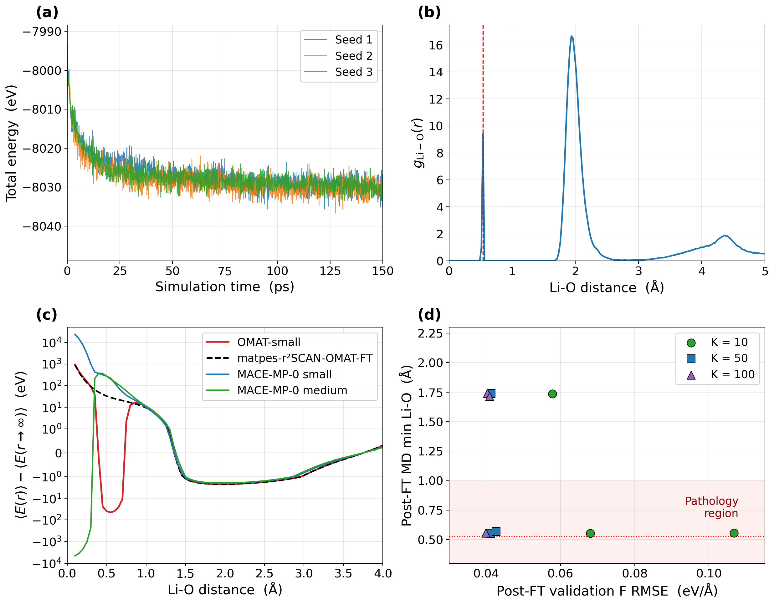
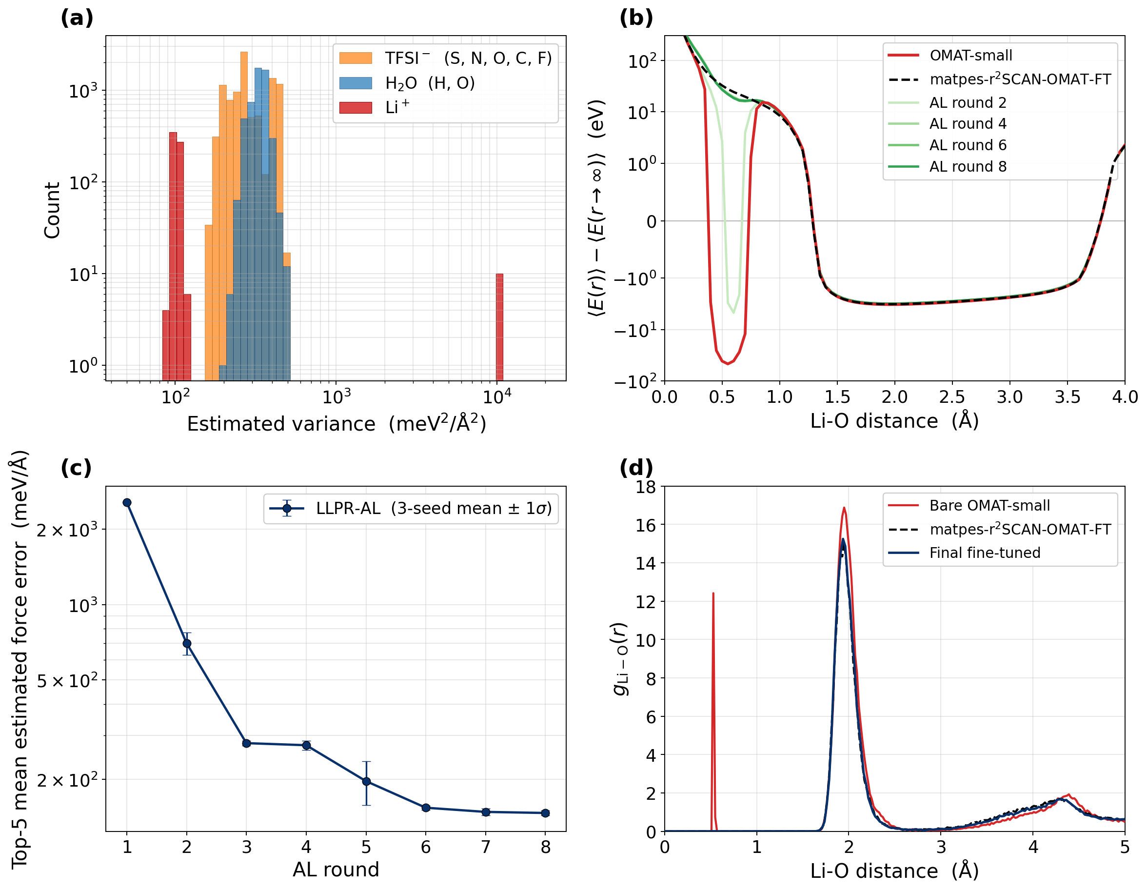
We first run three independent 100 ps NPT simulations at 300 K with the bare OMAT-small foundation on the 21 m LiTFSI electrolyte configuration. The trajectories are stable by standard MD diagnostics. The total energy is conserved to within thermostat tolerance across the full 100 ps (Figure 4a), and no numerical instability occurs. The density converges to 1.59 g/cm\(^3\), about 7% below the experimental value of 1.7126 g/cm\(^3\) for 21 m LiTFSI at 298 K[38]. The radial distribution function of Li–O, however, shows a persistent sub-angstrom peak that should not be there (Figure 4b): a single ion is locked at a 0.53 Å contact with an adjacent water O (see Figure 4b inset) throughout the trajectory, while the physically-expected first-shell peak at 1.97 Å is unchanged. The Li–O potential-energy scan (see Methods) in Figure 4c traces the cause: the OMAT-small PES has a hallucinated attractive well at 0.55 Å, roughly 45 eV below its long-range value. This is probably because Li–O contacts below \(\sim\)​1.5 Å are essentially absent from the OMAT24 pretraining set[9], so the network freely extrapolates its learned Li–O attractive prior into the unsampled short-range region without any architectural constraint forcing repulsion. The matpes-r\(^2\)SCAN-OMAT-FT reference has been independently benchmarked on 21 molal LiTFSI and shown to reproduce the experimental density, ion/solvent diffusion coefficients, and X-ray structure factor[39], and its Li–O PES is free of the OMAT-small short-range pathology (Figure 4c). This supports using it as the labelling oracle in our active-learning workflow and confirms that fine-tuning on r\(^2\)SCAN labels is sufficient to repair the OMAT-small pretraining pathology.

Previous benchmarking of foundation MLFFs on 21 m LiTFSI has shown that the matpes-r\(^2\)SCAN-OMAT-FT foundation accurately reproduces the experimental thermodynamic and dynamical properties of this electrolyte[39], and its Li–O PES is physically correct (Figure 4c). We therefore adopt it as a pseudo-oracle to label active-learning samples instead of running DFT. The goal here is not to develop a production force field for 21 m LiTFSI but to test whether a hallucinating foundation can be repaired by fine-tuning. To test whether standard fine-tuning diagnostics can detect the OMAT-small hallucination, we perform one-shot fine-tunings on K = 10, 50, and 100 random picks from the foundation’s hallucinated MD trajectory, labelled with matpes-r\(^2\)SCAN-OMAT-FT, with three retraining seeds per K. The fine-tuning recipe follows the same multihead template as before (details in Methods). Figure 4d plots the nine fine-tuned models by final validation force RMSE (the standard fine-tuning diagnostic, \(x\)-axis shown in meV/Å for figure-readability) against post-fine-tuning MD minimum Li–O distance (a deployment-quality probe). The K = 10 fine-tunes span a wider range of validation force RMSE (0.058–0.107 eV/Å), as expected at the data-limited end of the K-sweep. By K = 50 and K = 100, the six fine-tunes improve to a validation force RMSE of approximately 0.040 eV/Å, which would conventionally be considered accurate enough. The post-fine-tuning MD outcomes, however, are inconsistent even at K = 100: in five of the nine retraining seeds the model inherits the foundation pathology despite a converged-looking fine-tuning. Whether a fine-tune resolves the hallucination or not depends only on the random seed; the hallucination therefore cannot be reliably cured by one-shot fine-tuning, and standard fine-tuning diagnostics are uncorrelated with deployment-MD physicality in this foundation–target mismatch regime.

The LLPR-based uncertainty supplies the missing detection signal that the validation loss cannot. Computing the per-atom force uncertainty of the bare OMAT-small foundation on its hallucinated-MD trajectory, we find that almost every atom is in the in-distribution range (median \(\sigma_F \approx 300\) meV/Å); the exceptions are the Li atoms locked at the pathological 0.53 Å contact, whose \(\sigma_F\) extends in a long tail to roughly 10,000 meV/Å (Figure 5a). The signal distinguishes a configuration on which the foundation is interpolating from one on which it is extrapolating, which the validation-set loss cannot do because the validation set is drawn from the same hallucinated MD as the training set. The detection requires no DFT labels: it uses only the foundation’s own features and training-set covariance. Therefore, one can identify the foundation hallucination before committing to any labelled data.

We then run iterative LLPR-based active learning with the following steps. Each round picks 10 frames from the current MD ranked by the mean of the five largest per-atom force uncertainties, labels them with the matpes-r\(^2\)SCAN-OMAT-FT pseudo-oracle, accumulates them with the previous picks, and fine-tunes from the OMAT-small foundation with the multihead recipe (see Methods). The workflow is run for eight rounds with three independent retraining seeds. Figure 5b shows the Li–O potential-energy scan, comparing the bare OMAT-small foundation against the LLPR-based active-learning fine-tunes at rounds 2, 4, 6 and 8 alongside the matpes-r\(^2\)SCAN-OMAT-FT reference. By round 2 the hallucinated well has been substantially lifted but a shallow residual attraction at \(\sim\)​0.7 Å remains; by round 4 the curve has converged to a smooth physical Li–O potential with a steep short-range repulsive wall, and rounds 6 and 8 are essentially indistinguishable from each other. Figure 5c plots the per-round per-frame top-5 mean uncertainty error averaged across the three retraining seeds. It falls rapidly from approximately 2300 meV/Å at round 1 to about 700 meV/Å at round 2, 280 meV/Å at round 3, and stabilises at approximately 150 meV/Å from round 6 onwards. This convergence of the uncertainty error to an essentially constant value provides a natural stopping criterion for the active-learning loop. Figure 5d shows the Li–O radial distribution function from production NPT trajectories at 300 K and 1 atm comparing the bare OMAT-small foundation, the fine-tuned model at round 8 (3-seed mean), and the matpes-r\(^2\)SCAN-OMAT-FT reference. The pathological 0.53 Å peak is gone in the fine-tuned model, and its Li–O RDF closely tracks the matpes-r\(^2\)SCAN-OMAT-FT reference across the full range. The three-seed mean equilibrium density of the fine-tuned model at round 8, \(1.705 \pm 0.044\) g/cm\(^3\), agrees with both the matpes reference value of \(1.720\) g/cm\(^3\) measured under the same protocol and the experimental value of \(1.7126\) g/cm\(^3\)[39], confirming that the workflow produces a model capable of reproducing the reference behaviour on a structural and thermodynamic property the active-learning signal was not explicitly trained to fit.

Taken together, the workflow recovers production-quality molecular dynamics for the 21 m LiTFSI system from a deliberately mismatched foundation. Approximately 50 fine-tune labels distributed across eight active-learning rounds are sufficient to mitigate the hallucination that one-shot fine-tuning could not lift.

Discussion↩︎

Data efficiency is central to machine-learning force field training. In the train-from-scratch regime, a handful of well-picked configurations are equivalent in downstream accuracy to a dataset orders of magnitude larger, and our results show that this label-reduction effect carries through to the foundation fine-tuning regime. There, although a pretrained foundation already offers good out-of-the-box accuracy on many systems, deploying it on a new target chemistry still demands a carefully constructed fine-tuning dataset to cover the configurations the target system samples in MD. Beyond the label-cost concern, there is a second concern that is unique to the foundation paradigm. Pathological extrapolation arises when the target chemistry falls outside what the foundation has actually seen during pretraining, and these failures can persist silently into deployment if not specifically probed. A model committee is commonly used in active learning to flag such pathologies, but it requires training \(N\) independent MLFFs and is therefore costly even in the train-from-scratch setting; at foundation scale it becomes impractical, since each member is a full extra training run on a multi-million-configuration corpus. We show in this work that the last-layer-projection-regression (LLPR) framework[30], [31], equipped with a target-relevant covariance and a per-round absolute-units estimation, provides a lightweight forward-pass uncertainty signal that addresses both concerns across the three deployment regimes we examined and achieves full-data accuracy with substantially fewer DFT labels in both the train-from-scratch and the foundation fine-tuning settings.

In the train-from-scratch setting on a structurally heterogeneous water/ice candidate pool, the LLPR-driven workflow reaches the full-data-trained ceiling using only K = 100 labelled picks, an order of magnitude fewer labels than the 3955-frame full-data baseline. The LLPR picker is roughly twice as sample-efficient as random and competitive with the model committee at substantially lower compute, with cross-seed variance tight enough that picks made with a single trained model match the reproducibility of those from a multi-seed committee.

In the foundation fine-tuning setting on the same water/ice dataset, the picker effect transfers cleanly. Energy-LLPR picking on the MACE-MP-0 small foundation reaches its full-pool fine-tuning ceiling at K = 100, while random picking remains a factor of two to five away from the ceiling at the same K. Crucially, the bare performance gap between MACE-MP-0 small and MACE-MP-0 medium (more than fourfold at zero-shot) closes within K = 100 LLPR picks, showing that, in this test, which frames are labelled matters more than which foundation is used.

In the realistic deployment regime where no DFT-labelled pool exists by hypothesis (the 21 m LiTFSI electrolyte case), LLPR plays a different role. The bare OMAT-small foundation produces molecular dynamics that is stable by standard MD diagnostics yet structurally wrong, with a ion locked at a 0.53 Å contact with water that the foundation’s own PES has hallucinated as an attractive well. The LLPR per-atom uncertainty flags this hallucination directly on the affected frames before any labels are committed, drives the iterative active-learning loop, and self-terminates it via an absolute-units exit criterion set against the thermal-force scale. Fewer than fifty fine-tune labels suffice to recover production-quality molecular dynamics with an equilibrium density consistent with experiment and a Li–O coordination consistent with the r\(^2\)SCAN reference.

By integrating last-layer-projection regression uncertainty into the active-learning workflows used to train and fine-tune MLFFs, we show that full-data accuracy can be reached with substantially fewer labels and that the model’s own internal signal can drive an end-to-end workflow. The workflow is implemented in the open AI\(^2\)-kit[25] active-learning framework and supports both train-from-scratch and foundation fine-tuning pipelines; it is currently demonstrated on the MACE foundation family but the per-atom-feature hooks on which it relies generalise straightforwardly to other equivariant foundation architectures. Compared with the model committee, which requires \(N\) independently trained MLFFs and returns an uncertainty that is only relative across members, LLPR provides a quantitatively accurate, deterministic uncertainty from a single trained model, matching the committee on picker performance at a fraction of the compute. By establishing uncertainty quantification as a unifying interface between data selection, deployment-quality detection, and self-termination of the active-learning loop, this work brings foundation-model fine-tuning for atomistic chemistry one step closer to a routine and reliable workflow.

Methods↩︎

LLPR validation on bulk water↩︎

The DeePMD bulk-water model is trained on 50 frames of 64-water configurations sampled from the dataset of ref. [34], using the DeePMD-kit smooth-edition descriptor with a [240, 240, 240] fitting network, 5000 training steps under Adam (lr \(= 5 \times 10^{-4}\), annealed to \(10^{-7}\)). The held-out evaluation pool comprises 965 in-distribution 64-water frames, 1022 out-of-distribution 63-water frames, and 40 out-of-distribution 128-water frames, with the OOD subsets chosen as cell-size shifts of the training-set chemistry.

For each configuration \(x\), the last-layer activations of the DeePMD fitting network are hooked to produce a feature vector \(h_a(x)\) per atom \(a\) (sum-pooled per frame for the energy signal). Given a reference set \(\{x_i\}\), the per-atom feature covariance \(\Sigma_a\) is accumulated and regularised to give an inverse-covariance matrix \(A\); the per-atom leverage \(u_a(x)\) then measures how far the atomic feature lies outside the training distribution: \[\Sigma_a = \sum_{i,a} h_a(x_i)\,h_a(x_i)^\top, \quad A = \tfrac{1}{N_\text{tot}}\Sigma_a + \sigma_F^2 I, \quad u_a(x) = h_a(x)^\top A^{-1} h_a(x), \label{eq:llpr}\tag{1}\] with the Tikhonov ridge \(\sigma_F = 5 \times 10^{-3}\) throughout. The energy-LLPR uncertainty \(\sigma^2_E(x)\) is defined analogously on the sum-pooled per-frame features against a per-frame covariance, and the force-LLPR uncertainty is the per-frame mean of the five largest per-atom \(u_a\).

Train-from-scratch active learning on water/ice↩︎

The water/ice dataset[32], [33] (7241 RPBE-D3 configurations) is partitioned as follows: the bootstrap MLFF\(_0\) is trained on 1000 liquid-water frames; the active-learning candidate pool is the 1140-frame ice partition; the multi-phase test set is 990 frames (500 liquid + 490 ice); the from-scratch full-data ceiling trains on a 3955-frame union of the bootstrap, the active-learning pool, and the remaining small-cell liquid and ice frames not held out for testing. The 2296 large-cell frames are reserved as additional cell-size OOD probes (Table S2). The DeePMD bootstrap and retraining recipes are identical to the bulk-water case above.

Four picker strategies are compared: random sampling, energy LLPR (top-K by \(\sigma^2_E\)), top-5 force LLPR, and model committee. Each picker selects \(K \in \{50, 100, 150, 200\}\) frames from the candidate pool. Each retrained model is warm-started from the bootstrap and trained on a 200-frame liquid anchor plus the top-K active-learning picks. Three independent retraining seeds are run per (picker, K) cell.

Foundation fine-tuning on water/ice↩︎

The bootstrap MLFF\(_0\) of the previous subsection is replaced by the MACE-MP-0 foundation[10] (MP-0 small as the primary foundation, MP-0 medium for a model-size comparison); the active-learning candidate pool, multi-phase test set, and full-data ceiling training set are unchanged. Fine-tuning is done by MACE’s multihead approach[10], in which a Default head fits the active-learning set and a pre-train head reproduces the foundation on a replay dataset constructed from all MPtrj frames of H/O-only composition (7000 frames total). The loss is \(\mathcal{L} = w_E (E_\text{pred} - E_\text{ref})^2 + w_F |F_\text{pred} - F_\text{ref}|^2\) with \(w_E = w_F = 100\). The optimiser is AdamW with lr = \(10^{-4}\), EMA decay 0.99, weight decay \(5 \times 10^{-7}\), for 20 epochs per K cell. The MACE-MP-0 H and O atomic-energy references are re-aligned to the RPBE-D3 reference by a per-element linear regression on 200 liquid-anchor frames.

Iterative LLPR-based active learning on 21 m LiTFSI electrolyte↩︎

The target system is a 21 molal LiTFSI water-in-salt configuration: 1534 atoms per cell (64 , 64 TFSI\(^-\), 170 H\(_2\)O). Labels are produced by the matpes-r\(^2\)SCAN-OMAT-FT foundation[39], which has been independently benchmarked on 21 m LiTFSI and reproduces the experimental density, ion/solvent diffusion coefficients, and X-ray structure factor.

Calibration. The K = 10 picks of round \(k\) are an unbiased held-out set for the LLPR signal of the previous round’s model. On these picks we fit the geometric-mean estimator \[C_\text{geom} = \exp\!\left(\langle \log(e_a^2 / u_a) \rangle_a\right), \qquad \sigma_F(a;x) = \sqrt{C_\text{geom}\cdot u_a(x)}, \label{eq:Ccalib}\tag{2}\] where \(e_a\) is the per-atom force error of the previous round’s model against the pseudo-oracle labels, \(u_a\) is the LLPR leverage of Eq. 1 , and \(\sigma_F\) is the resulting absolute per-atom force-error uncertainty in eV/Å. The loop terminates when the 99th percentile of \(\sigma_F\) over a round’s MD samples falls below a user-chosen threshold (set to 100 meV/Å in this work, matching the 300-K thermal-force scale on a 1500-atom cell).

Foundation MD audit and Li-O scan. For the failure-mode audit we ran three independent NPT trajectories of the bare MACE-OMAT-small foundation on the 21 m LiTFSI electrolyte initial configuration (the nearest Li-O pair having an initial distance ranging from 0.8 to 2.5 Å across the 64 Li ions), with independent Maxwell-Boltzmann velocity seeds. Each trajectory ran 100 ps at a 0.5 fs timestep. The temperature was maintained at 300 K using the Nosé-Hoover thermostat with a relaxation time of 0.05 ps. The Melchionna barostat[40] was employed to maintain a pressure of 1 atm, with a relaxation time of 0.75 ps and a reference bulk modulus of 2.2 GPa. The rigid Li-O potential-energy scan (Figs. 4c, 5b) is performed on five representative MD frames per model: in each frame we pick the closest Li-O pair, displace the chosen Li along the Li-O axis through 79 distances \(r \in [0.10, 4.00]\) Å with all other atoms frozen, and evaluate the model’s potential energy at each \(r\). Curves are averaged across the five frames and re-zeroed at the average energy over \(r > 3.5\) Å.

One-shot and iterative active learning. The nine one-shot fine-tunes (\(K \in \{10, 50, 100\}\) random picks with 3 retraining seeds each) use the shared multihead template described above with the OMAT-small foundation and a 20,000-frame Li-bearing OMAT24 pre-train head replay. The iterative LLPR-based active-learning loop (Algorithm S1) runs as follows per round: (1) NPT MD for 10 ps at 300 K, 1 atm from the previous round’s final frame, sampling 100 snapshots from the last 5 ps at 50 fs spacing; (2) build the per-atom feature covariance from the prior reference (round 1: 2000 Li-bearing OMAT24 frames as foundation-domain proxy; from round 2 onwards: the accumulated active-learning set); (3) score frames by the top-5 force-LLPR uncertainty and pick \(K = 10\); (4) label picks with the matpes-r\(^2\)SCAN-OMAT-FT oracle and accumulate; (5) fit \(C_\text{geom}\) and check whether the uncertainty error is below the exit threshold; (6) if not exited, fine-tune the foundation on the accumulated active-learning set under the multihead template. Three independent random seeds (42, 123, 777) are run.

Production MD. For the production validation we ran 500 ps NPT trajectories at 300 K, 1 atm for four models (bare OMAT-small, LLPR-based active-learning final-round, random-picker final-round, matpes-r\(^2\)SCAN-OMAT-FT), with three independent velocity seeds per model. NPT settings are the same as above. Density, minimum Li-O distance, and Li-O, Li-N, and O-O radial distribution functions are computed on the last-200-ps trajectories.

Data and code availability↩︎

The datasets, trained model checkpoints, and scripts used in this work are available from the authors on reasonable request. They will be released open-source on Zenodo upon publication.

References↩︎