Immediate 3D Gaussian Splat Reconstruction of Unordered Input with Global Consistency
July 16, 2026
Abstract
3D Gaussian Splatting (3DGS) has become the method of choice for reconstructing and real-time rendering of captured scenes. To capture a scene with good visual quality, continuous image sequences are usually combined with out-of-order shots for better scene coverage. Structure from motion can reconstruct such captures, but only after they are all available and often with high computational cost. Incremental reconstruction methods – often derived from SLAM solutions – provide immediate feedback, but cannot handle the out-of-order capture we require. We provide the first immediate feedback solution for such radiance field capture that provides global consistency. We first introduce a method for fast matching in out-of-order sequences, by repurposing visual place recognition models and a covisibility graph, and provide an efficient way to find highly connected keyframes, improving quality even for ordered sequences. We show how these steps – together with GPU optimization and careful Gaussian primitive placement – provide fast local reconstruction, in our challenging radiance field reconstruction case. We then introduce a novel cluster-based method, again using the covisibility graph, to provide efficient loop closure that does not require sequential input. Finally, to handle large scenes in our context, we introduce a progressive hierarchy that allows our method to scale to large environments, without compromising efficiency. Our results show we provide immediate feedback 3DGS reconstruction with good visual quality in several datasets, with up to thousands of input images.
<ccs2012> <concept> <concept_id>10010147.10010371.10010372.10010373</concept_id> <concept_desc>Computing methodologies Rasterization</concept_desc> <concept_significance>500</concept_significance> </concept> <concept> <concept_id>10010147.10010371.10010396.10010400</concept_id> <concept_desc>Computing methodologies Point-based models</concept_desc> <concept_significance>500</concept_significance> </concept> <concept> <concept_id>10010147.10010178.10010224.10010245.10010255</concept_id> <concept_desc>Computing methodologies Matching</concept_desc> <concept_significance>500</concept_significance> </concept> <concept> <concept_id>10010147.10010178.10010224.10010245.10010254</concept_id> <concept_desc>Computing methodologies Reconstruction</concept_desc> <concept_significance>500</concept_significance> </concept> <concept> <concept_id>10010147.10010178.10010224.10010245.10010253</concept_id> <concept_desc>Computing methodologies Tracking</concept_desc> <concept_significance>500</concept_significance> </concept> </ccs2012>
1 Introduction↩︎
Radiance fields, and in particular 3D Gaussian Splatting (3DGS), have seen impressive adoption in the last few years [1], with applications in many different fields such as VFX, architecture, e-commerce, virtual reality, etc. Creating a good quality 3DGS reconstruction typically involves unordered capture: users often take photos moving around abruptly, turning, or coming back to the same place to cover the entire scene. Immediate feedback during capture is extremely important, allowing the user to determine if the capture is complete and of good quality. Unfortunately, no solution exists that allows immediate feedback for typical 3DGS capture patterns. We introduce a method that provides immediate feedback, and can handle the typical capture style required for 3DGS.
A vast majority of previous work on 3DGS assumes that camera poses are provided as input, typically using Structure from Motion (SfM) [2]. Recently there has been interest in immediate feedback, most often building on visual Simultaneous Localization and Mapping (SLAM) solutions [3], [4]. These, and methods that also create 3D Gaussians [5] assume that images are provided in sequential order, so that an incoming frame can be matched with a set of immediately preceding frames. This assumption is also made for SLAM methods (and mixed 3DGS methods [6]) that perform loop closure [7]. Both poses and Gaussians need to be updated when loop closure occurs, without compromising interactivity. Even efficient GPU-friendly approaches [5] cannot scale to the unordered case since more keyframes are needed for bundle adjustment (BA). All of these issues are exacerbated when handling large scenes with thousands of images as input.
Providing immediate feedback for unordered 3DGS captures raises several problems. First, instead of just trying to match an incoming frame to the last few preceding ones, matches potentially must be found in the entire set of previously registered frames. For this, we first introduce a fast, two-level matching algorithm building on visual place recognition [8] and learned features [9]. Once matching pairs are validated, we use a weighted covisibility graph—originally developed for loop closure [10]—to allow fast extraction of subsets of well-connected frames (i.e., with many matches) that can be distant in time. Second, we need to perform fast local reconstruction in our context. To allow bundle adjustment to scale while still exploiting the GPU effectively, we use the covisibility graph to restrict problem size and random sampling to maintain fixed size. This, together with several GPU optimizations, allows us to maintain immediate feedback in this more complex setting, as well as efficient updates of Gaussian primitives. Third, we need to handle loop closure, without the convenience of ordering where time can be used to detect loops. We introduce a cluster-based approach, using our fast subset extraction, allowing us to robustly identify when the user comes back to a part of the scene already captured. We propose a cluster-based “welding" scheme and an optimization-free method to efficiently propagate the update due to loop closure to poses and Gaussian primitives. Finally, we handle large scenes, which would quickly saturate VRAM if we apply our solution naively, since we would need to keep all keyframes. For this, we introduce a progressive hierarchy, determining which Gaussians do not contribute to the current frame, and consequently finding which keyframes to use for online optimization. The hierarchy also allows real-time rendering of such large scenes.
In summary, our contributions are:
A fast matching approach for unordered input for efficient retrieval of well-connected subsets of keyframes, allowing GPU-friendly local reconstruction.
Cluster-based loop detection for unordered sequences, with efficient optimization-free updates of poses and Gaussian primitives.
A progressive hierarchy for large scenes that allows efficient optimization and rendering accommodating limited GPU resources.
Our experiments show we can handle the vast majority of datasets previously used for 3DGS, while providing immediate feedback during capture. Such datasets cause previous online methods to fail. Our method also improves ordered capture.
2 Related Work↩︎
We briefly cover closely related work on novel view synthesis, offline and incremental pose estimation/reconstruction including for 3D Gaussian Splatting and global consistency. Each is a vast field on its own, and we refer the reader to surveys available, respectively [11], [12], [13]–[15] and [16].
2.0.0.1 Novel View Synthesis
Capturing real scenes from photographs or video —allowing subsequent free-viewpoint navigation— has seen impressive growth and adoption since the introduction of Neural Radiance Fields (NeRFs [17], [18]). NeRFs have a large computational overhead for volumetric ray tracing and neural network evaluation that was overcome by 3D Gaussian Splatting (3DGS) [19] and the numerous follow-up solutions [12]. Recently, feed-forward radiance field methods have been proposed (e.g., [20]–[23]), but these solutions are based on direct image prediction, have few guarantees on reconstruction accuracy and are usually limited in the number of images they can process.
Initial radiance field solutions focused on small environments since handling larger scenes requires many hours of processing [24]. Several solutions have been proposed for 3DGS, typically introducing a hierarchy [25]–[27]; these data structures require a preprocessing step and are thus not suitable in our immediate feedback context.
A few recent approaches are compatible with progressive reconstruction [5], [28], [29], but expect ordered input and do not handle loop closure. In contrast, our approach allows global consistency with progressive reconstruction.
2.0.0.2 Offline pose estimation for Radiance Field Reconstruction
NeRF and 3DGS methods frequently assume that camera poses were already reconstructed. This is typically achieved using Structure from Motion (SfM) pipelines like COLMAP [2]. Such methods fundamentally expect all images to be available before processing begins. They typically build maps incrementally by reordering images based on connectivity and use expensive —but accurate— exhaustive matching processes. These solutions (e.g., [2], or the more recent [30]) use global bundle adjustment, enabling high quality and globally consistent reconstructions, handling loop closure. Unfortunately, this comes at a high computational cost, because joint optimization of poses and landmarks scales poorly. Direct solvers for the Schur complement exhibit cubic complexity in the number of cameras in the worst case, while iterative methods like PCG [31] reduce per-iteration cost but require more iterations as the problem conditioning degrades with size. Although hierarchical approaches such as COLMAP’s Hierarchical Mapper improve scalability, they remain fundamentally offline processes, making them unsuitable for the strict latency constraints of interactive capture. This precludes the use of such solutions to treat poses for large scenes and achieve immediate feedback. Recent learning-based approaches have received attention, and in particular multiview-transformer solutions [32], [33]; however, these still have significant computation overhead and limited accuracy, making them unsuitable in our context.
2.0.0.3 Incremental Reconstruction and 3DGS
Visual SLAM methods
[15] have been developed in the different context of robotics and fundamentally process frames sequentially,
exploiting temporal consistency for efficiency. Typically, only a small window of previous frames is used as a constrained feature search window to register a new image, and motion priors can be exploited. This limits robustness in the case of fast motion
which is common for radiance field capture. There is a vast body of research on ordering and relocalization such as ORB-SLAM [10], using
bag-of-words [34]. These methods treat tracking and relocalization as distinct modes, pausing reconstruction when tracking is lost. Instead, we
continuously search for the best possible matches. Most SLAM systems use CPU-based local bundle adjustment via Ceres [35] or g2o [36]. GPU-accelerated alternatives exist for dense systems like DROID-SLAM [37] or large-scale sparse problems [31], [38]. DROID-SLAM’s system
density hurts performance and the sparse solvers show large overhead and cannot optimize shared camera intrinsics due to their solver structure. Hierarchical methods for SLAM (e.g., [39]) are based on scene graphs; we propose a cluster-based approach specific to unordered input, and overall repurpose SLAM tools for radiance field capture with immediate feedback.
Several methods integrate Gaussian Splatting with pose estimation, but most rely on external SLAM backends [3], [4] and inherit their limitations. End-to-end approaches exist but are either slow [40]–[42] or restricted to limited camera motion, with no relocalization or loop closure [5], [43]. Others are demonstrated on ordered input [44]–[49]. Some recent work focuses on specific input modalities (stereo [50], RGB-D [51], RGB-LIDAR [52]). We introduce several new solutions to improve the quality of the incremental joint optimization of poses and 3D Gaussians from unordered RGB input, while maintaining efficiency.
2.0.0.4 Global Consistency
Loop closure detection and pose graph optimization offer a more lightweight alternative to global bundle adjustment by optimizing poses only from loop closure constraints, but the methods typically remain iterative [16], [53], [54]. Specific solutions have been explored, e.g., targeted to building semantics [55] or using RGB-D inputs [56]; we target a more general algorithm. Neural SLAM methods show promise (e.g., [7]) but current solutions do not yet achieve the performance/accuracy levels we require. LoopSplat [6] corrects a Gaussian splat reconstruction by rigidly transforming primitives after loop closure, but targets RGB-D input and cannot handle scale drift inherent to monocular systems. Our solution for global consistency builds on our covisibility graph, allowing an efficient optimization-free method to deform the trajectory via graph traversal, avoiding iterative optimization over all poses, and updating landmarks and Gaussians with scale taken into account.
3 Overview↩︎
For each incoming keyframe, we estimate its pose by matching against previously registered keyframes and running bundle adjustment, then back-project Gaussians and refine the representation. Unlike sequential captures where matching against a short temporal window is sufficient, unordered input requires efficiently searching the entire history for overlapping views, correcting drift on revisits, and bounding GPU memory as the scene grows. We first perform a fast two-level matching approach and create a covisibility graph, together allowing us to quickly find well-connected subsets of keyframes from the entire registered sequence. Second, we introduce a fast, GPU-optimized local bundle adjustment used for pose estimation; a set of local Gaussians is jointly initialized and optimized per keyframe. Third, we present a graph-based solution for loop closure that propagates changes using our covisibility graph and proposes a fast optimization-free update for poses and Gaussians. Finally, we present a progressive hierarchy for large scenes. We present each component next. A pipeline overview figure and pseudocode of the full algorithm are provided in the appendix, along with further algorithmic details for each step.
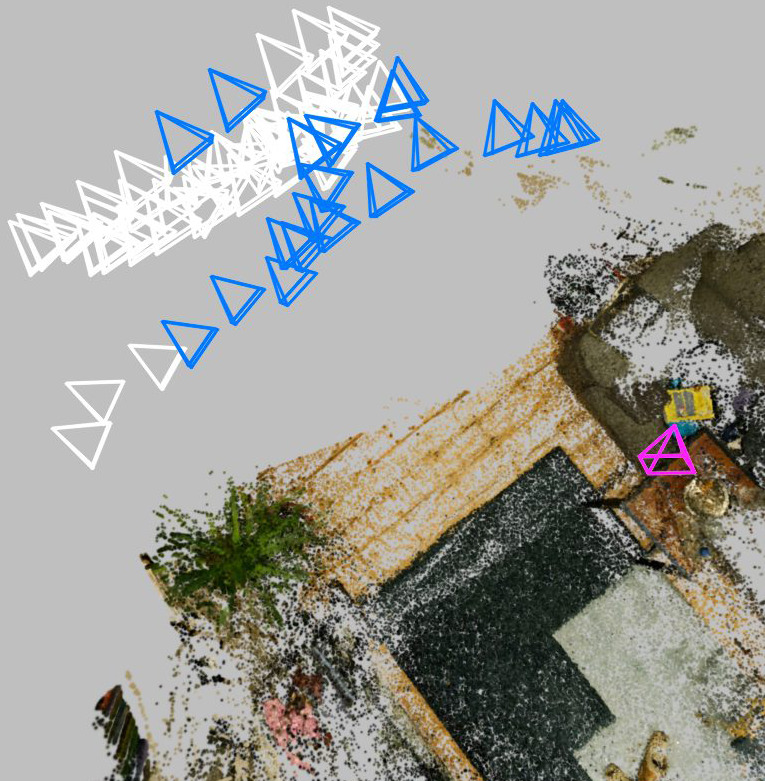
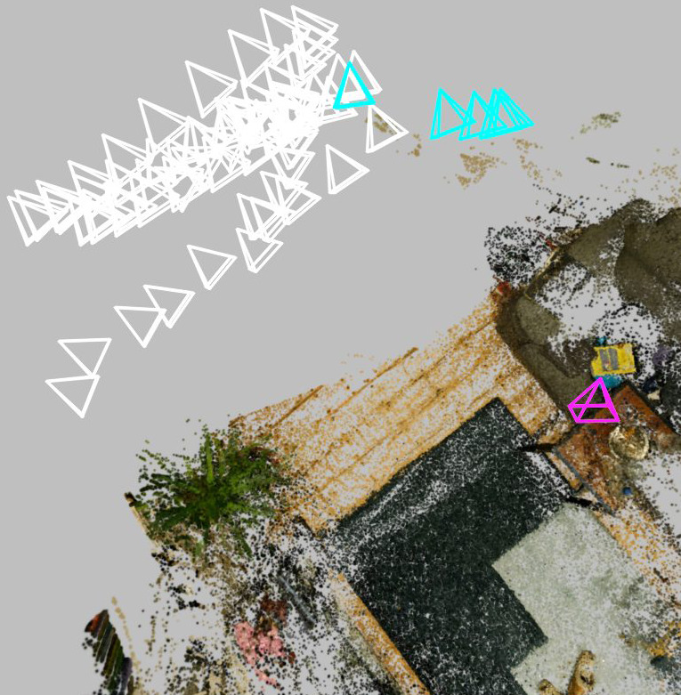
Figure 1: We show an intermediate sequence of registered frames for the MipNeRF360 room scene. In white are all registered frames, and in magenta is the incoming frame \(I_q\), which is out of order.Left we show in blue the \(\mathcal{K}=20\) images selected by MixVPR and right we show in cyan the \(\mathcal{K}'=5\) images selected with brute-force matching and validated as pairs..
4 Fast Out-of-order Matching↩︎
Typical radiance field captures include abrupt motion around the scene, potentially requiring all previous keyframes to be examined to match the incoming keyframe. This is prohibitively expensive even for moderately large scenes. To find reliable keyframe pairs with potential matches, we introduce an efficient, two-level matching approach that builds on relocalization and loop closure tools for ordered sequences. We then need to select good keyframes to use for local reconstruction (Sec. 5): for this we use a weighted covisibility graph [10] with a greedy traversal. The graph is also central for global consistency (Sec. 6.1), allowing efficient pose update propagation.
4.1 Efficient Two-level Matching↩︎
For a new incoming (or query) keyframe \(I_q\), we need to find the best candidates for matching from all previously registered keyframes. Our two-level matching approach first uses a learned visual place recognition model, MixVPR [8], to retrieve the \(\mathcal{K}\) most similar keyframes for each incoming frame. Importantly, MixVPR extracts a 4096-dimensional global descriptor \(\mathbf{d}\) for each image that can be compared to previously registered frames via cosine similarity, making it efficient for very large-scale retrieval.
Formally, the similarity between query frame \(I_q\) and a registered keyframe \(I_i\) is \(s(I_q, I_i) = \mathbf{d}_q \cdot \mathbf{d}_i\), where \(\mathbf{d}_q\) and \(\mathbf{d}_i\) are the respective normalized global descriptors. We retrieve the top-\(\mathcal{K}\) candidates as \(\mathcal{K} = \text{top-K}\{s(I_q, I_i) \mid I_i \in \mathcal{M}\}\), where \(\mathcal{M}\) is the set of all registered keyframes, using \(\mathcal{K}=20\).
Given this efficient preliminary step, we run a first round of geometric verification on the \(\mathcal{K}\) candidates using brute-force feature matching with XFeat [9], a fast and robust local feature extractor, retaining the \(\mathcal{K}'\) keyframes with the highest inlier count: \(\mathcal{K}' = \text{top-K'}\left\{\left|\mathcal{I}_i^{\text{BF}}\right| \mid I_i \in \mathcal{K}\right\}\), where \(\mathcal{I}_i^{\text{BF}}\) is the set of brute-force matches between \(I_q\) and \(I_i\), and \(\mathcal{K}'=5\). We then perform accurate matching on this reduced set using LightGlue [57], ensuring efficiency through mixed precision and CUDA graphs. A pair is validated if it yields more than \(\tau_{m} = 500\) inliers after RANSAC with a fundamental matrix model: \(\mathcal{V} = \left\{I_i \in \mathcal{K}' \mid \left|\mathcal{I}_i^{\text{LG}}\right| > \tau_{m}\right\}\), where \(\mathcal{I}_i^{\text{LG}}\) is the set of LightGlue matches between \(I_q\) and \(I_i\). A visualization can be seen in Fig. 1.
Our matching is a speed/quality cascade: MixVPR matches at \(\approx\)1ms/1000 pairs, XFeat at \(\approx\)0.5ms/pair, and LightGlue+RANSAC at \(\approx\)4ms/pair, with corresponding quality gains. Each stage filters for the next, so we can only afford the slower and more accurate methods on progressively smaller candidate sets.
This solution robustly tracks frames even when they are added out of order, or when revisiting places after a long time, without requiring a dedicated relocalization module. We maintain the speed required for immediate feedback and in addition we select the most relevant keyframes even for ordered sequences.
4.2 Weighted Co-visibility Graph↩︎
A key element of our solution is the ability to quickly identify and access most closely linked keyframes, both for local matching of an incoming frame but also to rapidly determine keyframes needed in loop closure (Sec. 6.1). We solve this by constructing a weighted covisibility graph [10] to represent the connectivity between keyframes based on their shared observations. Each node in the graph corresponds to a keyframe, and an edge is created between two nodes if the pair has been validated: we add the edges between \(I_q\) and \(\mathcal{V}\) into the graph \({G} = (\mathcal{M}, E, W)\) after each new frame is tracked. The edge weight is defined from the number of inlier matches between the two keyframes: \(w_{ij} = \frac{1}{\#\text{inliers}(i,j)}\). A higher number of inliers indicates a stronger geometric relationship, i.e., a lower weight. These weights allow us to prioritize stronger connections with efficient graph traversal algorithms, which is useful for local reconstruction, our solution for loop closure with clustering (Sec. 6.1) and for efficient drift correction (Sec. 6.3).
4.3 Finding Well-connected Subsets in the Graph↩︎
Both choosing keyframes for local bundle adjustment (Sec. 5.1), and finding keyframes on both sides of a loop closure (Sec. 6.2), require the selection of sets of keyframes that are strongly connected. We leverage the covisibility graph for this. We first describe connectivity-based keyframe selection for a new incoming frame \(I_q\); we explain how it generalizes later.
We consider an active set of nodes \(\mathcal{S}_t\), initialized with the incoming frame \(I_q\). In the graph, \(I_q\) is connected to the validated pairs as explained above. We then start a greedy graph traversal, to find the nodes (keyframes) that are strongly connected to \(I_q\). At each step, we add a node that has (locally) maximum connectivity to the active set \(\mathcal{S}_t\). To find the node to add, we visit all candidate nodes, i.e., all nodes connected to a member of \(\mathcal{S}_t\). We compute the total connectivity \(c\) of each such node \(I_i\) to \(\mathcal{S}_t\), where connectivity is defined as: \(c(I_i, \mathcal{S}_t) = \sum_{I_j \in \mathcal{S}_t} \#\text{inliers}(i,j)\). We then choose the node \(I_i\) with the maximum cumulative inliers, which can be written as: \[\mathcal{S}_{t+1} = \mathcal{S}_t \cup \left\{\operatorname{argmax}_{I_i \in \mathcal{M} \setminus \mathcal{S}_t} c(I_i, \mathcal{S}_t)\right\}\]
We continue with such steps until we have the desired number of keyframes \(N\), which depends on the use case (see Fig. 2). Given that each graph node has a small number of connections (around 10 in our experiments), this greedy approach is very efficient.
None
Figure 2: Finding well-connected subsets with a greedy algorithm: From a starting frame \(I_q\) (magenta), we expand the set \(\mathcal{S}_t\) (gray) iteratively by considering the direct neighbors and including the node with the largest combined connectivity (indicated by strength of connection)..
5 Efficient Local Pose and Gaussian Reconstruction↩︎
In the following, we use the terms observations for the 2D screen locations of matched features and landmarks for the 3D points of matched features. When reconstruction starts, we bootstrap our model by exhaustively matching the first 8 well-connected keyframes, rectifying outliers using Lambda Twist [58] on the GPU as a minimal P3P solver for RANSAC. We then use Depth Anything 3 [23] to initialize poses, focal length and landmarks, fixing inaccuracies in them with local bundle adjustment (BA).
5.1 Local Bundle Adjustment↩︎
At each incoming frame, we perform local BA. We first use the approach described above (Sec. 4.3) to select \(N=20\) keyframes, often far back in time in the set of registered keyframes. This is a higher number of keyframes than previous methods that either consider direct matches only (ORB-SLAM) or a temporal window (5 frames for DROID-SLAM), since the out-of-order problem is harder; the challenge is to be robust while maintaining efficiency.
To allow efficient GPU BA, we need to use a fixed set of landmarks. For this we perform multinomial sampling based on the number of observations per landmark to randomly select the \(K\) landmarks from those that are observed by at least two of the selected keyframes (\(K=10000\) in our tests). We follow standard practice to fix \(n_f\) keyframes that are used in the loss but not optimized (we use \(n_f=4\)). We randomly choose these from the \(N\) selected keyframes, which proves to be robust in practice.
5.1.0.1 Solver efficiency
Previous fast BA solutions [5] are efficient and accurate for very small problems (\(N=5\)), but do not scale for the \(N=20\) keyframe case we have. We address this limitation while maintaining the GPU efficiency by allowing each landmark to be observed by a fixed subset of keyframes in the local window, selected based on covisibility. Furthermore, we implement GPU kernels for residual and Jacobian computation, and maintain a dense Schur complement formulation, which shows better performance than sparse solvers in our context. We achieve 5\(\times\) speedup against existing CPU and GPU optimizers [5], [36], [38] (Sec. 8).
5.2 Gaussian Placement and Optimization↩︎
After a keyframe pose is estimated and refined with local BA, new Gaussian primitives are added to the reconstruction. Recent methods place Gaussian primitives using learned depth predictors with a scale and offset factor, typically computed once for the entire image [26]. This, however, is often inaccurate [59]. To overcome this limitation, we split the images into tiles, and compute a scale and offset for each tile. We then upsample with linear interpolation to match the input resolution. This provides much finer correction to the predicted depth, improving the quality of the positions chosen for the Gaussians (see Sec. 9).
Using this depth, we follow [5] in spawning new Gaussians. These Gaussians are directly linked to the keyframe, allowing later loop closure events (Sec. 6.1) to update the radiance field. For fast optimization, the full Gaussian model is trained for 30 iterations using a custom differentiable renderer based on [60], sampling nearby views (see Sec. 7.2). We fix 30 iterations per keyframe for reproducible evaluation; for live capture we instead run optimization asynchronously until the next keyframe is added.
5.3 Dealing with Unmatchable Keyframes↩︎
When there is no visual overlap to the registered keyframes, pose estimation will fail. In this case, we “shelve" the keyframe to be retried later. When the cosine similarity of the shelved keyframe’s visual descriptor compared to the registered keyframes becomes large, the keyframe is unshelved and retried. This efficiently introduces a reordering scheme to avoid failure cases and allow disjoint sequences to be eventually matched. An exception to this is if the keyframe was unmatched because of low parallax, estimated with the triangulation angle. In this case, we disregard it as we also assume it to contribute little to the reconstruction quality.
6 Out-of-order Global Consistency↩︎
Reconstruction error accumulates over time, resulting in drift. Loop closure is required to correct the drift, and consolidate everything into the same space. Traditional ordered sequence loop closure uses time stamps to identify if the candidate has not been seen recently, simplifying loop closure detection; in the out-of-order setting, this is no longer possible.
To solve this problem we introduce clusters of keyframes for robust detection. When adding a new keyframe, we force the creation of two clusters of poses from the matched keyframes, the first one containing the new pose and poses connected to it. If there is a second cluster of poses that is sufficiently large and disconnected from the first —despite being matched— this indicates a set of poses that “see the same content”, thus requiring loop closure. We next use the clusters to robustly “weld” the respective poses, and propagate corrections efficiently with the graph to other poses and Gaussians.
6.1 Cluster-Based Loop Detection↩︎
We first take \(2K'\) best matches (Sec. 4.1), and create two separate clusters of keyframes \(\mathcal{C}_1, \mathcal{C}_2\). Selecting \(2K'\) allows clusters of size \(K'\) in both clusters if evenly distributed. We initialize the two clusters with the two keyframes that are the most distant in terms of connectivity. We run local reconstruction (Sec. 5) on the largest of the two clusters. To determine if the clusters are not sufficiently connected, we check the number of hops in the covisibility graph that separates them. If the clusters are separated by more than \(\tau_{lc}=5\) hops, and the smaller cluster has more than \(\tau_{v}=2\) pairs, a loop closure occurs.
Our approach does not require timestamps and is robust to small isolated match sets that are likely false positives. It makes local BA more robust by discarding small clusters, makes the connectivity graph more accurate and prevents loop closure false positives.
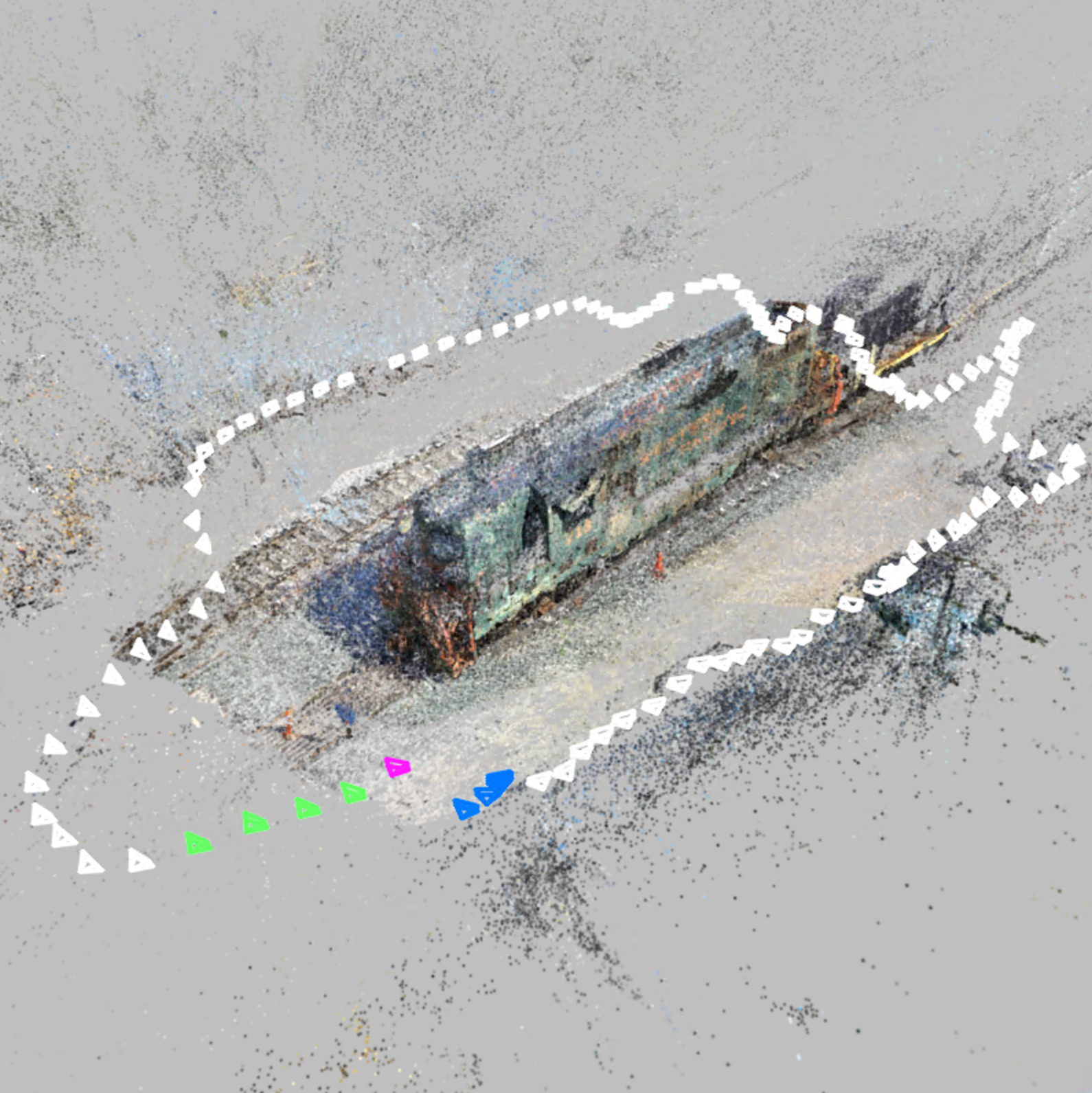

Figure 3: Left we show cluster-based loop closure in the train scene, in a (mostly) ordered scenario: blue poses are the new (free) cluster, while green are the fixed cluster. On the right, we use the same color coding, and we see that the two clusters come from disjoint, unordered sequences..
6.2 Welding Window Bundle Adjustment↩︎
Once a loop closure is detected, we have two clusters of keyframes that are in separate spaces, and that require poses to be reoptimized together. We use the notion of a “welding window” [10], but in the new context of keyframe clusters.
We perform BA on this welding window around the detected loop closure. We use our keyframe selection strategy (Sec. 4.3) to select the most relevant sets of keyframes on both sides of the loop closure, ensuring a more robust and accurate optimization. In this case, the initial set \(\mathcal{S}_t\) contains the keyframes of each cluster. We expand from there to select \(N/2\) keyframes on each side of the loop closure, allowing balanced optimization with our N-frames welding BA. We take the union of these expanded keyframe sets to define the welding window. We then run our efficient local BA (Sec. 5) over this window to optimize the poses and landmarks. To constrain landmark motion overall, we fix \(n_f\) keyframes in the older set. We need to fix one set for the propagation step below, so we fix the old one as we expect it is likely already well optimized, more stable, and connected to more of the trajectory; the other is called the free cluster.
6.3 Drift Correction by Propagation Through the Graph↩︎
Traditional solutions [53], [56], [61] use optimization to propagate corrections to the other poses after loop closure. We avoid this by exploiting our covisibility graph to efficiently find “most connected” keyframes providing reliable poses. We estimate a rigid transformation that is propagated efficiently to other poses, by determining a backbone path using Dijkstra’s algorithm in the covisibility graph.
In each cluster, we first select the set of most connected keyframes within the welding window \(\mathcal{W}\): these anchor keyframes have the most reliable pose. We then compute the rigid body transformation (SE(3)) between the initial and re-optimized pose for the anchor keyframe in the free cluster. To obtain the full similarity transformation \(\mathbf{S}_{\Delta} \in Sim(3)\), we estimate the scale change \(s_{\Delta}\) from landmark depth variations and compose it with the rigid transform. We now have one anchor in each cluster and the similarity transform between their previous and “welded” pose. To propagate this transformation to all poses efficiently, we first compute a backbone path composed of well-connected keyframes that are likely reliable, using Dijkstra’s algorithm to find the path with the smallest cumulative edge weights in the graph. Loop edges are not yet in the graph, so the backbone goes through existing connections only. We then distribute the computed Sim(3) transformation along the backbone path, proportionally to the geodesic distance to the optimized keyframe. We interpolate rotations with 6D representation [62] and scale using log interpolation.
Finally, we propagate the corrections to the rest of the trajectory by moving each keyframe following the transformation of the closest backbone keyframe in terms of geodesic distance, and applying the same correction. The most relevant backbone node for this keyframe is that with minimal geodesic distance. After loop closure, we add the loop matches to the covisibility graph (Sec. 4.2) so that they are used in subsequent local BA.
None
Figure 4: Loop Closure: (a) When a new keyframe (magenta) is matched (dotted lines) to distinct clusters of the graph, a loop closure is triggered. (b) These clusters extended with connected frames then define a local welding window (gray), in which BA is done with older keyframes fixed (grayed out). (c) The changes are then propagated through the minimal backbone of the graph, with other poses connected through spatial locality..
Each Gaussian primitive added keeps track of the keyframe that added it. We apply the same Sim(3) transformation as that used for the keyframe that created each Gaussian, and we update scale and rotation accordingly.
| TUM | MipNeRF360 | StaticHikes | ||||||||||
| PSNR\(^\uparrow\) | SSIM\(^\uparrow\) | LPIPS\(^\downarrow\) | Time\(^\downarrow\) | PSNR\(^\uparrow\) | SSIM\(^\uparrow\) | LPIPS\(^\downarrow\) | Time\(^\downarrow\) | PSNR\(^\uparrow\) | SSIM\(^\uparrow\) | LPIPS\(^\downarrow\) | Time\(^\downarrow\) | |
| Photo-SLAM | 19.30 | 0.700 | 0.382 | 0:02:12 | 16.54 | 0.505 | 0.603 | 0:02:11 | 14.13 | 0.316 | 0.660 | |
| MonoGS | 16.60 | 0.682 | 0.381 | 0:16:18 | 14.46 | 0.436 | 0.663 | 0:04:05 | 15.46 | 0.301 | 0.659 | 0:09:19 |
| On-The-Fly NVS | 23.02 | 0.821 | 0.250 | |||||||||
| S3PO-GS w\refinement | 21.88 | 0.777 | 0.309 | 1:29:04 | 19.82 | 0.553 | 0.576 | 0:23:29 | 18.09 | 0.368 | 0.611 | 0:54:44 |
| LongSplat | 1:41:08 | 23.63 | 0.657 | 0.415 | 2:25:26 | 20.05 | 0.461 | 0.481 | 22:40:56 | |||
| Ours | 0:02:14 | |||||||||||
| G+T3DGS (7k) | 25.29 | 0.868 | 0.191 | 0:03:33 | 27.52 | 0.866 | 0.226 | 0:08:50 | 20.23 | 0.537 | 0.465 | 1:02:34 |
| MipNeRF360 | Tanks and Temples | Deep Blending | ||||||||||
| PSNR\(^\uparrow\) | SSIM\(^\uparrow\) | LPIPS\(^\downarrow\) | Time\(^\downarrow\) | PSNR\(^\uparrow\) | SSIM\(^\uparrow\) | LPIPS\(^\downarrow\) | Time\(^\downarrow\) | PSNR\(^\uparrow\) | SSIM\(^\uparrow\) | LPIPS\(^\downarrow\) | Time\(^\downarrow\) | |
| Ours | 25.60 | 0.772 | 0.270 | 0:01:28 | 21.42 | 0.774 | 0.252 | 0:01:37 | 23.83 | 0.813 | 0.290 | 0:01:47 |
| G+T3DGS (7k) | 27.08 | 0.815 | 0.262 | 0:09:57 | 21.90 | 0.779 | 0.271 | 0:05:13 | 25.80 | 0.855 | 0.268 | 0:05:36 |
| SmallCity* | Wayve* | CityWalk | ||||||||||
| PSNR\(^\uparrow\) | SSIM\(^\uparrow\) | LPIPS\(^\downarrow\) | Time\(^\downarrow\) | PSNR\(^\uparrow\) | SSIM\(^\uparrow\) | LPIPS\(^\downarrow\) | Time\(^\downarrow\) | PSNR\(^\uparrow\) | SSIM\(^\uparrow\) | LPIPS\(^\downarrow\) | Time\(^\downarrow\) | |
| H3DGS | 21.17 | 0.679 | 0.285 | 2:55:28 | 20.80 | 0.737 | 0.227 | 7:29:45 | 11.78 | 0.557 | 0.560 | 22:09:20 |
| Octree-GS | 1:20:59 | 0.313 | 2:21:48 | 17.33 | 0.638 | 0.520 | 3:11:40 | |||||
| S3PO-GS w\refinement | 19.71 | 0.652 | 0.462 | 0:57:31 | 17.81 | 0.644 | 0.423 | 1:25:26 | 10.72 | 0.439 | 0.579 | 6:00:28 |
| On-The-Fly NVS | 23.59 | 0.789 | 0.323 | 0:01:45 | 20.29 | 0.739 | 0.303 | 0:04:29 | 21.71 | 0.712 | 0.395 | 0:25:03 |
| Ours | 23.56 | 0.800 | 0.302 | 0:02:25 | 23.04 | 0.822 | 0.234 | 0:04:12 | 22.03 | 0.772 | 0.336 | 0:29:38 |
7 A Progressive Gaussian Hierarchy↩︎
Processing large scenes for 3DGS requires some form of hierarchy [25], [26]. Such solutions require a substantial computational overhead to create or update the hierarchy that we cannot afford. We propose a hierarchical structure that is fast to build and update, based on primitive screen size. A node holds Gaussian parameters (position/opacity/rotation/scale/SH coefficients), and parent/children IDs. These enable going coarser or finer within the hierarchy, depending on required precision. Active nodes’ Gaussian parameters are optimized with the rendering loss. At a given point in time, small footprint leaf Gaussian primitives will be offloaded to the CPU RAM, freeing up VRAM for the optimization. However, this poses challenges during progressive reconstruction.
7.1 Adaptive Gaussian Merging and Retrieval↩︎
We maintain an active set of Gaussian primitives at any time, which contains leaf as well as intermediate nodes that result from merging. We analyse the hierarchy every time a new keyframe is added, computing \(S_i\), the screen size of each Gaussian \(G_i\), from the current viewpoint. We merge small, subpixel Gaussians with \(S_i < \tau_l = 0.5\) pixels, and only trigger merging when more than \(20\%\) of the Gaussians fit this criterion to avoid too frequent merging.
Within the set of primitives selected for merging, we get the 4 closest Gaussians using a fast KNN search [63] and remove duplicates to prevent a Gaussian primitive from having multiple parents. Merging is performed by groups of 4 Gaussians using KL-divergence based merging [26]. We then update the hierarchy by removing sub-pixel Gaussians from the active set, and adding new parent Gaussians, together with child-parent links. If a Gaussian already has a parent, we check if all children of this parent need to be merged; if so, we pull the parent from the hierarchy instead of creating a new node. We can now optimize a smaller set of Gaussians, and can handle large scenes with limited GPU memory. When loop closure occurs we move all Gaussians in the hierarchy following the transform of the keyframe most used to spawn its children; this is done asynchronously to avoid affecting latency.
When navigating, if a merged node contributes more than \(\tau_h = 1\), we reload the finer Gaussians and update their coarse parent nodes. We then reload their children and remove these parent nodes from the active set, resulting in an active set sufficiently fine to represent the scene for the keyframe used to optimize or the frame to render. We use double buffering to avoid stutter.
7.2 Frame Selection and Rendering↩︎
During online optimization, we need to avoid frames that mostly see offloaded primitives and use keyframes that see leaf or small Gaussians. For this we sample keyframes using a probability based on the number of leaf Gaussians still in the active set that were generated by this keyframe. We keep at least 50 keyframes to have context and optimize intermediate nodes. We then remove keyframes that contribute \(< 5\%\) of the max contribution by offloading them to the CPU. Thanks to this scheme, intermediate hierarchy nodes are automatically optimized, not requiring explicit post-optimization.
We store the state hierarchy after optimization, and we can then reload it for rendering. We start with roots, i.e., nodes that do not have parents. We then descend in the hierarchy until nodes are finer than \(\tau = 1\), or we reach a leaf. As we do this, we continuously check if there are parents whose node would have \(S_i<\tau\) to potentially take a coarser node and offload Gaussians. This hierarchy traversal takes 5 to 30 ms per step depending on size, and is computed asynchronously with double buffering.
8 Results and Evaluation↩︎
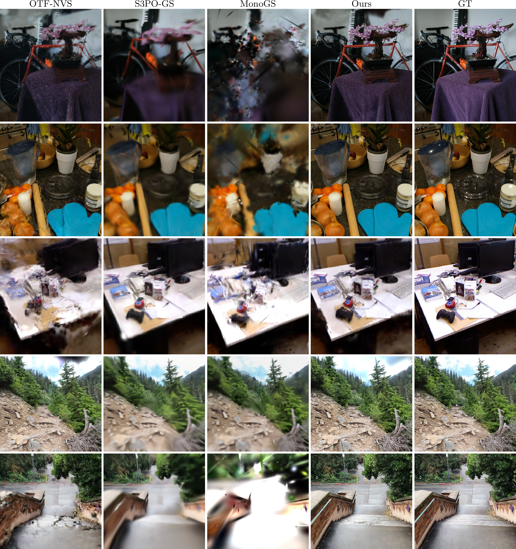
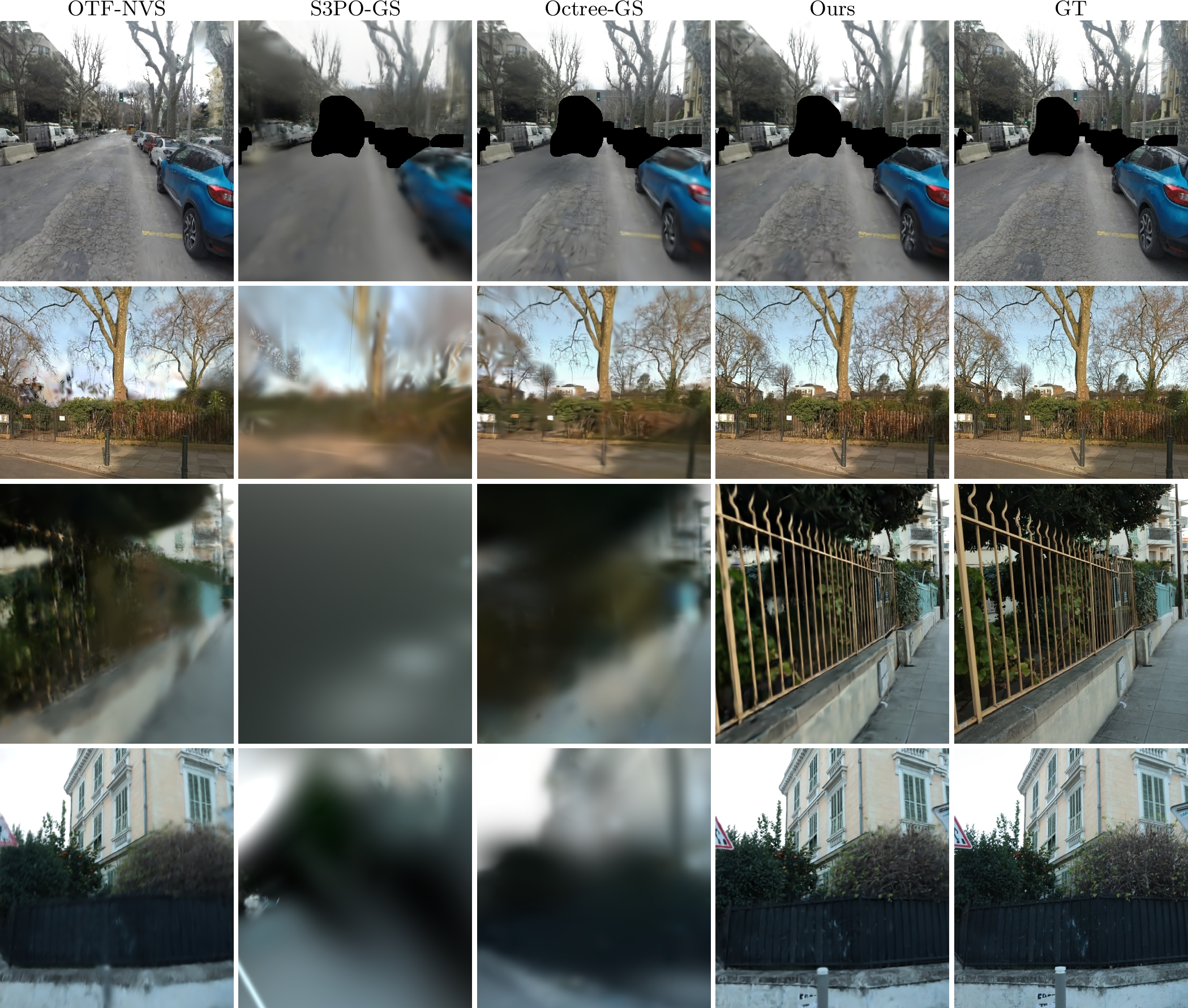
We present results and comparisons of our method in Fig. [fig:evaluation] and [fig:evaluation95large], illustrating that we provide fast reconstruction and maintain good visual quality; additional results can be found in the video.
8.1 Evaluation Methodology↩︎
We use the datasets and evaluation protocol as proposed in [5] for Tab. 1 and 3. We compare to the following previous methods: On-the-fly NVS [5], Photo-SLAM [4], DROID-Splat [3] and MonoGS [43], as well as S3PO-GS [44], LongSplat [40] and AnySplat [22]. AnySplat and DROID-Splat require resized images so we report these results separately in the appendix. For large scenes we compare to [5], H3DGS [26], Octree-GS [25] and S3PO-GS [44]. We also present evaluation on out-of-order scenes from the standard datasets MipNeRF360 [64], Tanks and Temples [65] and Deep Blending [66] in Tab. 2; here we just compare to COLMAP+3DGS, using the code from the official 3DGS repository that has TamingGS [60] acceleration for optimization, since all other pose-free methods fail for these scenes. We run evaluations on a workstation with an Intel Core i9 13900K CPU, 128GB of RAM, and an NVIDIA RTX 4090 GPU, or if we use a different configuration (e.g. when the method requires more GPU memory) we scale the timings to this setup by running our algorithm on Garden on each machine.
8.2 Comparisons↩︎
8.2.0.1 Ordered scenes
Tab. 1 summarizes our evaluation results. Among pose-free methods, our approach achieves faster reconstruction than all prior methods except [5], over which we obtain superior rendering quality. Our method outperforms all baselines in quality, with the exception of LongSplat on the TUM dataset; however, LongSplat requires 1h41min compared to 1min22sec for our method. LongSplat’s local optimization performs well at low resolution (\({\sim}0.3\) Mpx) and high frame overlap (e.g., TUM), but requires \({\sim}75\times\) more compute time and degrades on higher-resolution (\(>1\) Mpx), wider-baseline scenes (MipNeRF360, StaticHikes). GLOMAP+Taming3DGS struggles on the larger (\({\sim}1000\) frames, tens-of-meters trajectory) and more challenging StaticHikes scenes, as Taming3DGS lacks a level-of-detail scheme and adequate densification scheduling for large-scale inputs. Our method also shows better quality than AnySplat, even when AnySplat is augmented with additional optimization (see appendix). For large scenes, our method achieves superior quality across all evaluations, except for Octree-GS on the SmallCity scene; notably, COLMAP+Octree-GS requires 1h20min, compared to 2min25sec for our method. On SmallCity, our quality is comparable to OTF-NVS, though at higher computational cost.
We provide fine-tuning results with additional optimisation in the appendix.
20 epochs (+43s) suffice to reach GLOMAP+Taming3DGS (7k)’s quality.
On MipNeRF360, the average and maximum latency (defined as the time from start of processing to readiness for next frame) are 324 ms and 386 ms.
8.2.0.2 Pose estimation evaluation
We evaluate pose estimation quality and present the results in Tab. ¿tbl:tab:pose-eval?. Spann3R [67] is a transformer-based feed-forward 3D reconstruction method. We use poses provided by TUM and COLMAP as pseudo ground truth for MipNeRF360. Our method achieves high accuracy in wide baseline scenes while remaining competitive with dedicated SLAM methods on small baseline benchmarks.
1.5pt
8.2.0.3 Unordered scenes
Tab. 2 reports results on MipNeRF360, Tanks and Temples and Deep Blending, which contain a mix of ordered and unordered sequences within the same scene (e.g., Bicycle and Playroom) that the sequential comparisons above cannot handle. We achieve quality that is less than 3DGS at 7k iterations, but is still sufficiently high to be usable, as shown in the video. Overall, the total computation time required is around 6 times lower than this offline solution, which has higher quality nonetheless.
Figure 7:  .
.
Figure 8: 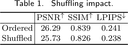 .
.
Figure 9: 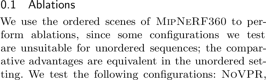 .
.
Figure 10: 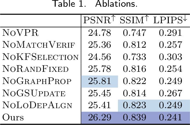 .
.
we match to the last five images instead of our out-of-order matching NoMatchVerif, we directly use the top-K from MixVPR without brute-force matching, NoKFSelection, we optimize the 20 last keyframes during local BA instead of our selection scheme, NoRandFixed, we fix the oldest cameras instead of randomize, NoGraphProp, we use PyPose’s PGO [68] instead of our faster graph propagation (here we focus on speed), NoGSUpdate, we do not move Gaussians after pose update in loop closure, NoLoDepAlgn, we use global scale and offset for monocular depth alignment instead of computing it locally, per tile. Ours is our full solution. From Tab. 10, we see that MixVPR and our keyframe selection have the biggest influence on quality overall. All other components contribute to improving the quality of the result, but in a less significant manner. The impact of each component on the pose quality is presented in the appendix.
8.2.0.4 Impact of the hierarchy
Hierarchy levels are created dynamically throughout the reconstruction, ranging from a single level for small scenes like MipNeRF360 to 8 levels for CityWalk. Processing CityWalk without hierarchy runs OOM (24GB GPU) after 795 out of 4050 frames (less than 20%) with 6.7 million Gaussians, while the hierarchy maintains the peak number of trained Gaussians below 3.7 million and allocated memory below 12.8 GB, improving training speed and enabling complete processing. See Tab. 8 in the appendix for more details.
9 Limitations↩︎
Our method trades a small quality gap vs. offline approaches for orders-of-magnitude faster processing. Pure rotations prevent triangulation, a limitation shared with methods from COLMAP to ORB-SLAM. While we show that graph-based propagation is not worse than global PGO (NoGraphProp ablation), it does not match slower global BA (e.g., GLOMAP). Failure cases are illustrated in Fig. [fig:limitations] of the appendix.
10 Conclusion↩︎
We have presented a method that enables immediate feedback for 3DGS reconstruction from unordered sequences typical of radiance field capture. To efficiently retrieve keyframes that may lie far back in capture time, we repurpose visual place recognition together with the covisibility graph traditionally used in SLAM for loop closure. We combine this with GPU optimization to perform fast and robust local bundle adjustment over substantially larger windows than in previous work. For loop closure, we propose a clustering approach suited to unordered input, leveraging the graph to perform optimization-free updates of both camera poses and Gaussian primitives. Finally, a lightweight progressive hierarchy allows our method to scale to large scenes. Together, these contributions yield the first complete solution that makes immediate feedback possible for high-quality radiance field capture.
This work was funded by the European Research Council (ERC) Advanced Grant NERPHYS, number 101141721 https://project.inria.fr/nerphys. Views and opinions expressed are however those of the authors only and do not necessarily reflect those of the EU or the European Research Council. Neither the EU nor the granting authority can be held responsible for them. The authors thank Adobe and NVIDIA for donations. Experiments presented in this paper were carried out using the Grid’5000 testbed, supported by a scientific interest group hosted by Inria and including CNRS, RENATER and several Universities and other organizations (https://www.grid5000.fr). This work was granted access to the HPC resources of IDRIS under the allocation AD011015561R1 made by GENCI.
11 Additional Method Details↩︎
11.1 Overview↩︎
Algorithm [alg:main] and Figure 11 provide an overview of our method.
\(\mathcal{M}\gets \emptyset\) \(G \gets (\emptyset, \emptyset, \emptyset)\) \(\mathcal{G} \gets \emptyset\) \(\mathcal{H}\gets \emptyset\) \(\textit{Shelf} \gets \emptyset\) Bootstrap first 8 well-connected keyframes
None
Figure 11: Overview of our proposed pipeline. Given an input image \(I_q\) sampled from an unordered image collection, we first apply a two-level matching strategy to establish correspondences. Images that cannot be matched are shelved for later processing. For matchable images, camera poses are estimated and refined via local bundle adjustment (BA), with loop closure aided by querying the covisibility graph to identify related keyframes. New Gaussian primitives are then instantiated and integrated into the scene hierarchy, followed by several optimization steps prior to the next input image..
11.2 Rotation Invariance in Matching↩︎
While robust, learned descriptors, especially those based on CNNs, are typically not rotation invariant and can only handle small rotations. To allow our method to handle a wide variety of data, even when frames are captured with strong rotation around the camera axis, we extract MixVPR and XFeat features for four different rotations of the image, with 90° steps. For XFeat keypoints, we only extract the keypoints in the upright image and sample the features in all of the four rotated images. For matching, we first quickly test rotation using MixVPR, before selecting the corresponding rotated XFeat features. Using MixVPR to detect orientation before XFeat and LightGlue allows us to maintain matching efficiency.
11.3 Details on Local Pose Reconstruction↩︎
11.3.0.1 Fast Bundle Adjustment
We employ a custom version of bundle adjustment (BA) for both local BA and welding window loop closure, which has to be very fast for our incremental reconstruction objective.
Previous fast BA solutions [5] are efficient and accurate only for very small problems (\(N=5\)), but do not scale: every landmark is observed by all keyframes in the local window, leading to a quadratic growth of the number of observations with respect to the number of keyframes. This occurs since the number of landmarks grows linearly with the number of keyframes. As a result such solutions are not sufficiently fast in our context with \(N=20\) keyframes. We address this limitation while maintaining the GPU-compatibility of the solver by allowing each landmark to be observed by a fixed subset of keyframes in the local window, selected based on covisibility. This reduces the number of observations significantly, enabling us to scale to larger local windows without sacrificing efficiency.
11.3.0.2 Shelving
Shelving is our solution to register disjoint sequences efficiently. When a new frame cannot be matched to any of the registered set, or if pose initialization fails, it is added to the shelf to process it later. We continuously compute the best MixVPR match between the shelved frames and the registered set. If the best match is above the cosine similarity of the last registered image, we attempt to add the shelved frame to the registered set. If frames remain in the shelf after the end of the capture, we process them starting from the best VPR match to the worst.
We interleave unshelving with new-frame processing, keeping the delay between capture and processing start below the time to handle two keyframes (\(<\)0.8 s).
11.4 Loop Closure Details↩︎
We employ loop closing when we detect disjoint clusters in the visual neighborhood through the covisibility graph.
11.4.0.1 Clustering
We define \(d_G(\mathcal{C}_1, \mathcal{C}_2) = \min_{I_i \in \mathcal{C}_1, I_j \in \mathcal{C}_2} \text{hops}(I_i, I_j)\) where \(\text{hops}(I_i, I_j)\) is the shortest path length in the covisibility graph. We also look at the size of the smaller cluster. We consider that a loop closure occurs if it has more than \(\tau_v\) valid pairs and the clusters are separated by more than \(\tau_{lc} = 5\) hops. Concretely, if: \[d_G(\mathcal{C}_1, \mathcal{C}_2) > \tau_{lc} = 5 \text{ and } \min(|\mathcal{C}_1|, |\mathcal{C}_2|) > \tau_v\] loop closure is triggered.
11.4.0.2 Welding Window
Formally, the welding window is defined as: \(\mathcal{W} = \mathcal{S}_{N/2}^{\mathcal{C}_{1}} \cup \mathcal{S}_{N/2}^{\mathcal{C}_{2}}\) where \(\mathcal{S}_{t}^{\mathcal{C}}\) is the set of \(t\) keyframes selected starting from cluster \(\mathcal{C}\).
11.4.0.3 Graph-Based Drift Correction
In each cluster, we first select the set of most connected keyframes within the welding window \(\mathcal{W}\): we can expect these anchor keyframes to have the most reliable pose after the welding BA: \[I_a^{1} = \operatorname{argmax}_{I \in \mathcal{S}_{N/2}^{\mathcal{C}_{1}}} c(I, \mathcal{W}), ~~~ I_a^{2} = \operatorname{argmax}_{I \in \mathcal{S}_{N/2}^{\mathcal{C}_{2}}} c(I, \mathcal{W})\] We then compute the rigid body transformation (SE(3)) between the initial and re-optimized pose for the anchor keyframe in the free cluster (i.e., the most recent keyframes): \[\mathbf{T}_{\Delta} = \mathbf{T}_a^{\text{opt}} \left( \mathbf{T}_a^{\text{init}} \right)^{-1}\] where \(\mathbf{T}_a^{\text{opt}}, \mathbf{T}_a^{\text{init}} \in SE(3)\) denote the optimized and initial poses of \(I_a^{1}\). To obtain the full similarity transformation \(\mathbf{S}_{\Delta} \in Sim(3)\), we estimate the scale change \(s_{\Delta}\) from landmark depth variations and compose it with the rigid transform: \(\mathbf{S}_{\Delta} = \text{Sim3}(\mathbf{T}_{\Delta}, s_{\Delta})\).
We now have one anchor in each cluster and the similarity transform between their previous and “welded” pose. We need to propagate this transformation to all poses efficiently. To do this we first compute a backbone path composed of well-connected keyframes that are likely reliable.
We build a backbone path between the two keyframes along the covisibility graph, using Dijkstra’s algorithm to find the path with the smallest cumulative edge weights: \[\mathcal{B} = \text{Dijkstra}\left(I_a^{1}, I_a^{2}, G\right)\] Note that loop edges have not yet been added to the graph, so the backbone goes through existing connections only. We then distribute the computed Sim(3) transformation along this backbone path, proportionally to the distance to the optimized keyframe: \[\alpha(I_b) = \frac{d_G\left(I_b, I_a^{2}\right)}{d_G\left(I_a^{1}, I_a^{2}\right)} \quad \forall I_b \in \mathcal{B}\] \[\mathbf{S}_{\Delta, b} = \text{interp}_{\text{Sim}(3)}(\mathbb{I}, \mathbf{S}_{\Delta}, \alpha(I_b))\] where \(\mathbb{I}\) is identity. We interpolate rotations with 6D representation [62] and scale using: \(s_{\Delta, b} = s_{\Delta}^{\alpha(I_b)}\).
Finally, we propagate the corrections to the rest of the trajectory by moving each keyframe following the transformation of the closest backbone keyframe in terms of geodesic distance, and applying the same correction. We get the most relevant backbone node for this keyframe as follows: \[I_{b^*} = \operatorname{argmin}_{I_b \in \mathcal{B}} d_G(I_i, I_b) \quad \forall I_i \notin \mathcal{W}\] and apply the transformation to the pose: \[\mathbf{T}_i^{\text{new}} = \mathbf{S}_{\Delta, b^*} \circ \mathbf{T}_i^{\text{old}}\]
After the loop closure has been treated, we add the loop matches to the covisibility graph so that they are used in subsequent local bundle adjustment.
11.4.0.4 Example
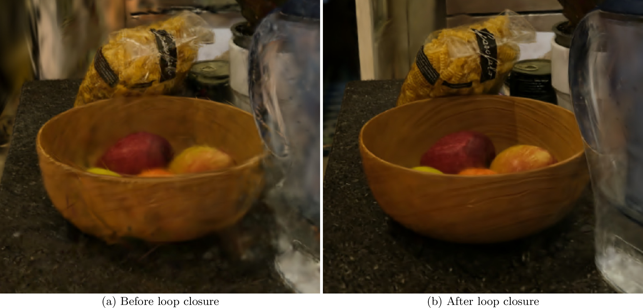
Fig. [fig:loop95c95example] shows an example on the Counter scene from the MipNeRF360 dataset. The accumulated drift is rectified via loop closure, and all Gaussians are updated. This allows the pipeline to optimize clean Gaussian models.
| TUM | MipNeRF360 | StaticHikes | ||||||||||
| PSNR\(^\uparrow\) | SSIM\(^\uparrow\) | LPIPS\(^\downarrow\) | Time\(^\downarrow\) | PSNR\(^\uparrow\) | SSIM\(^\uparrow\) | LPIPS\(^\downarrow\) | Time\(^\downarrow\) | PSNR\(^\uparrow\) | SSIM\(^\uparrow\) | LPIPS\(^\downarrow\) | Time\(^\downarrow\) | |
| Photo-SLAM | 19.30 | 0.700 | 0.382 | 0:02:12 | 16.54 | 0.505 | 0.603 | 0:02:11 | 14.13 | 0.316 | 0.660 | |
| MonoGS | 16.60 | 0.682 | 0.381 | 0:16:18 | 14.46 | 0.436 | 0.663 | 0:04:05 | 15.46 | 0.301 | 0.659 | 0:09:19 |
| On-The-Fly NVS | 23.02 | 0.821 | 0.250 | |||||||||
| S3PO-GS | 10.79 | 0.729 | 0.341 | 1:26:49 | 18.75 | 0.518 | 0.589 | 0:18:52 | 14.87 | 0.316 | 0.640 | 0:50:43 |
| S3PO-GS w\refinement | 21.88 | 0.777 | 0.309 | 1:29:04 | 19.82 | 0.553 | 0.576 | 0:23:29 | 18.09 | 0.368 | 0.611 | 0:54:44 |
| LongSplat | 1:41:08 | 23.63 | 0.657 | 0.415 | 2:25:26 | 20.05 | 0.461 | 0.481 | 22:40:56 | |||
| Ours | 0:02:14 | |||||||||||
| G+T3DGS (7k) | 25.29 | 0.868 | 0.191 | 0:03:33 | 27.52 | 0.866 | 0.226 | 0:08:50 | 20.23 | 0.537 | 0.465 | 1:02:34 |
3pt
| SmallCity* | Wayve* | CityWalk | ||||||||||
| PSNR\(^\uparrow\) | SSIM\(^\uparrow\) | LPIPS\(^\downarrow\) | Time\(^\downarrow\) | PSNR\(^\uparrow\) | SSIM\(^\uparrow\) | LPIPS\(^\downarrow\) | Time\(^\downarrow\) | PSNR\(^\uparrow\) | SSIM\(^\uparrow\) | LPIPS\(^\downarrow\) | Time\(^\downarrow\) | |
| H3DGS | 21.17 | 0.679 | 0.285 | 2:55:28 | 20.80 | 0.737 | 0.227 | 7:29:45 | 11.78 | 0.557 | 0.560 | 22:09:20 |
| Octree-GS | 1:20:59 | 0.313 | 2:21:48 | 17.33 | 0.638 | 0.520 | 3:11:40 | |||||
| S3PO-GS | 18.24 | 0.610 | 0.510 | 0:53:43 | 13.32 | 0.602 | 0.459 | 1:20:37 | 5.95 | 0.102 | 0.645 | 5:57:13 |
| S3PO-GS w\refinement | 19.71 | 0.652 | 0.462 | 0:57:31 | 17.81 | 0.644 | 0.423 | 1:25:26 | 10.72 | 0.439 | 0.579 | 6:00:28 |
| On-The-Fly NVS | 23.59 | 0.789 | 0.323 | 0:01:45 | 20.29 | 0.739 | 0.303 | 0:04:29 | 21.71 | 0.712 | 0.395 | 0:25:03 |
| Ours | 23.56 | 0.800 | 0.302 | 0:02:25 | 23.04 | 0.822 | 0.234 | 0:04:12 | 22.03 | 0.772 | 0.336 | 0:29:38 |
3pt
12 Additional Evaluations↩︎
12.1 Novel View Synthesis↩︎
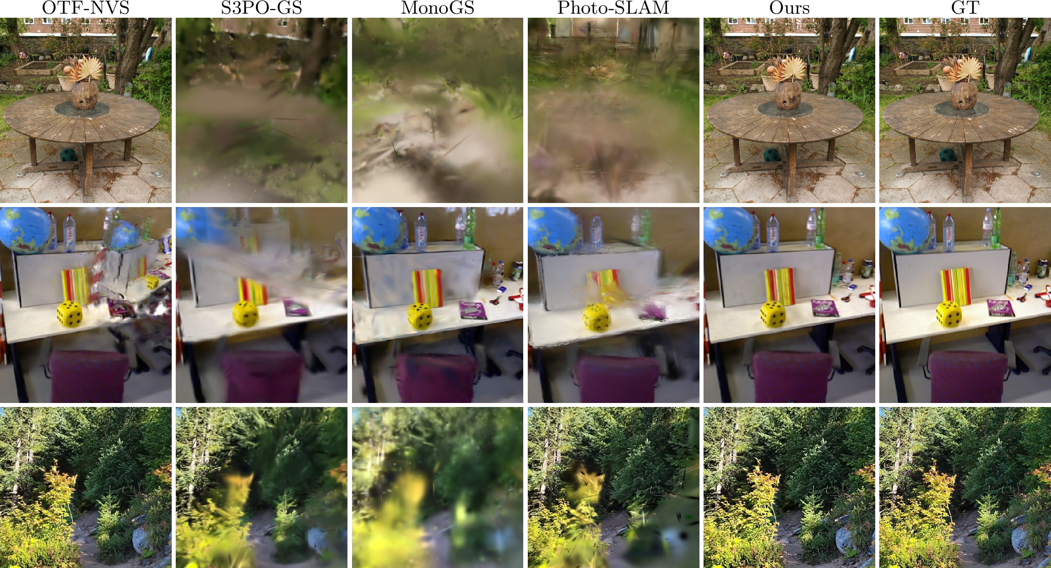
In addition to the numbers in the main paper, we present additional qualitative results (Fig. [fig:results95page95supp]) and metrics comparing S3PO-GS’s fast version without refinement in Tab. 4. As seen, while it provides good quality on the MipNeRF dataset with about 20% less training time, neither reaches our quality. Similar results can be seen on the large-scale scenes in Tab. 5.
12.1.0.1 Low resolution
DROID-Splat and CF-3DGS go OOM with full resolution images. Tab. ¿tbl:tab:slam-eval-low-res? shows results with images resized to 446x336 for TUM and 640 width for MipNeRF360 and StaticHikes.
12.1.0.2 AnySplat
AnySplat [22] provides a large vision model backbone and directly predicts Gaussians from images. This limits image sizes to \(448\times448\) pixels, and is quite expensive with regard to VRAM, limiting applicability: the method runs out of memory on an H100 on StaticHikes.
| PSNR\(^\uparrow\) | SSIM\(^\uparrow\) | LPIPS\(^\downarrow\) | Time\(^\downarrow\) | |
|---|---|---|---|---|
| AnySplat | 18.05 | 0.43 | 0.39 | 0:00:25 |
| AnySplat +1k | 21.53 | 0.60 | 0.30 | 0:02:10 |
| Ours | 24.98 | 0.81 | 0.21 | 0:00:40 |
1.5pt
In Tab. 6, we compare our approach in this low-resolution setup on the MipNeRF360 dataset. Both the feed-forward setup and the 1K iteration post-optimization method described by them fail to reach our quality.
12.1.0.3 Fine-tuning
Table ¿tbl:tab:fine-tuning? shows the results of fine-tuning after the initial reconstruction on MipNeRF360.
3pt
12.2 Additional Ablations↩︎
12.2.0.1 Hyperparameter sensitivity
Tab. ¿tbl:tab:hyperparam? shows the sensitivity of our method to \(\tau_{lc}\) and \(\tau_v\) on MipNeRF360.
3pt
12.2.0.2 Ablations on unordered scenes
We provide additional ablations on MipNeRF360 including unordered scenes (Tab. ¿tbl:tab:unordered95ablations?).
3pt
12.2.0.3 Pose quality ablation
The impact of remaining components on the pose estimation quality is shown in Tab. ¿tbl:tab:pose95ablations?. Note that NoGSUpdate and NoLoDepAlgn have no impact on pose estimation and are therefore excluded from the table.
3pt
12.2.0.4 VPR robustness
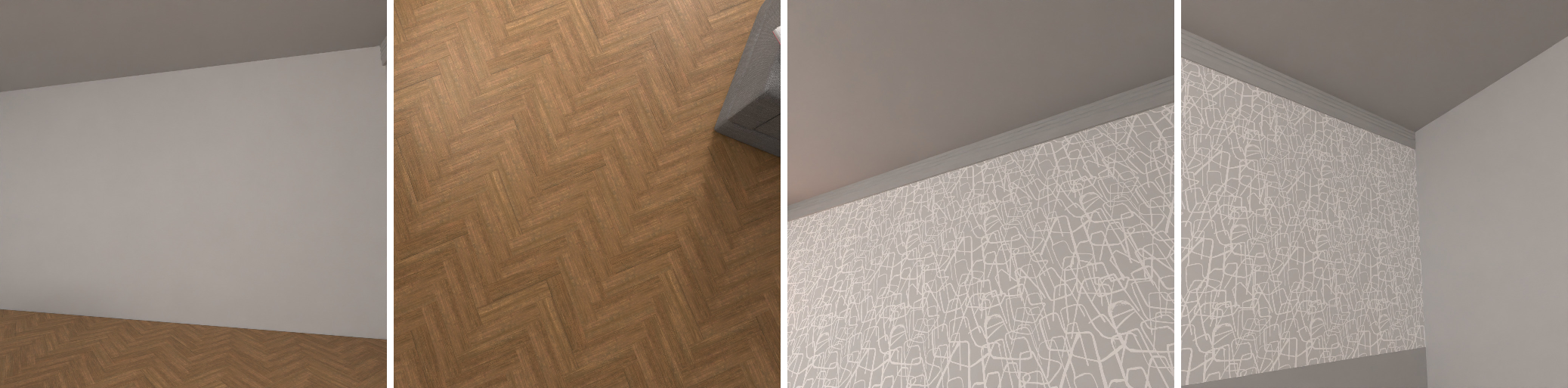
In all scenes tested, none failed due to VPR thanks to geometric verification (XFeat+LightGlue+RANSAC), which eliminates false positives. Top-5 by MixVPR and by geometric inliers have overlap in 100% of frames on MipNeRF360, and 92% on a synthetic scene with artificial repetitions and low-texture areas (Fig. [fig:repeat]).

12.2.0.5 BA runtime
We compare our bundle adjustment solution with state-of-the-art BA solvers in g2o [36], CudaBA [38] and the MiniBA of [5] on a synthesized problem. As seen in Tab. 7, our solution convincingly outperforms all other solutions in speed.
| g2o | CudaBA | On-The-Fly | Ours | |
| Runtime (ms) | 461.4 | 78.1 | 79.7 | 15.9 |
12.2.0.6 Hierarchy and memory scaling
Tab. 8 summarizes peak number of trained Gaussians and peak GPU memory with and without our progressive hierarchy on StaticHikes (medium-sized) and CityWalk (large-scale). We sample these metrics each time new Gaussians are added, reporting GPU memory used by PyTorch-allocated tensors. On medium-sized scenes the hierarchy brings a 38% reduction in peak number of Gaussians, while on CityWalk processing without it is infeasible.
| StaticHikes | CityWalk | |||
| #GS | Mem | #GS | Mem | |
| w/o hierarchy | 2.1 M | 8.8 GB | >6.7 M\(^{\dagger}\) | OOM (\(>\)24 GB)\(^{\dagger}\) |
| w/ hierarchy | 1.3 M | 6.2 GB | 3.7 M | 12.8 GB |
4pt
\(^{\dagger}\)Reached after 795/4050 frames before OOM.
12.3 Limitations↩︎
Fig. [fig:limitations] shows failure cases of our method. We use the fr1/rpy rotation-only sequence from TUM, originally captured for RGB-D SLAM evaluation where depth removes the need for triangulation, and the Train scene from Davis [69].