Per-Token Fixed-Point Convergence in Depth-Recurrent Transformers
July 15, 2026
Abstract
A depth-recurrent transformer applies a weight-tied core a variable number of times, and prior work has shown that training with a randomized recursion count yields one checkpoint usable across a range of inference depths. We ask what such a model actually computes per token, and measure it directly. On a 135M-class model trained on FineWeb-Edu, the recurrent state converges to a per-token fixed point: mean successive-output KL divergence falls from \(3.9\times10^{-1}\) at the second loop to \(8.5\times10^{-6}\) by the sixteenth, and per-token state change decays in step. Crucially, this convergence is not uniform across tokens. The median token converges by loop six, while approximately 10 percent of tokens continue to update at the training-mean depth of eight, and mean convergence depth is ordered by token type (whitespace shallowest, content words deepest). This per-token variation is the central object of the paper. We show it is directly readable and that reading it outperforms learning to predict it: a training-free rule that halts each token once its output stabilizes attains uniform depth-8 quality at 4.94 average loops (a 38 percent reduction in average depth) and matches uniform depth across the average-depth range, whereas a linear router trained on convergence labels harvested from the same model requires nearly full depth and yields no reduction. The elasticity that makes this possible reproduces here as background (validation loss decreases monotonically from 3.80 at one loop to 3.20 at eight and remains stable to 32 loops). We report average depth as a FLOP proxy with a three-point wall-clock bracket rather than a realized speedup, make no FLOP-matched parity claim, and note that the allocation results are established at a single scale and seed. The complete study runs on a single RTX 4090 in approximately 100 GPU-hours.
1 Introduction↩︎
A fixed-depth transformer binds its quality to a single compute operating point. Serving several quality and cost tiers requires training, storing, and operating several models, and adapting compute to input difficulty requires switching among them at inference, which forfeits the prompt cache. Both costs share a cause: depth, the primary determinant of per-token compute, is fixed in the weights.
Depth-recurrent transformers, which apply a weight-tied block a variable number of times [1], [2], relax this constraint. A single parameter set can in principle operate at many depths, so one training run can cover a range of compute budgets, and the depth can be selected per request or per token at inference. Whether this holds in practice depends on two properties that prior work often conflates. The first is depth robustness: whether the model produces useful output at depths for which it was not specifically tuned. The second is depth allocation: given a robust backbone, how much depth each token should receive, and whether the allocation policy must be learned jointly with the model.
Prior work leaves a gap at this seam. Per-token early exit on non-shared stacks stalled on the key-value cache and on batching: a token that permanently skips deep layers writes no keys or values there, so later tokens have nothing to attend to, and the published methods sacrifice one of input adaptivity, cache correctness, or compute savings [3]–[5]. Mixture-of-Recursions [6] trains the depth router and the compute budget together at pretraining time, which fixes the budget in the weights; the router saturates and cannot be retargeted afterward. Huginn [2] shows that randomized-depth pretraining produces a depth-robust backbone at 3.5B parameters, but it sets a single global depth by hand at inference and does not characterize its own emergent stop rule or test whether a learned policy could beat it. LoopFormer [7], concurrent with this work, improves the training objective for elastic depth but allocates a single global budget per sequence and names per-token budgeting as a limitation. Jointly trained halting has an established history: adaptive-computation methods that learn a halting policy alongside the model [8], [9] are known to collapse to degenerate depths and to require delicate tuning of a compute prior [10]. In each case, depth allocation is either fixed manually, applied globally per sequence, or learned jointly with the model, and in none of these lines is the per-token computation of a trained elastic model measured directly. We take that measurement as the starting point: we hold a randomized-depth backbone fixed, characterize how its recurrent state evolves per token, and ask what the simplest policy that reads this behavior achieves relative to a policy trained to predict it.
We separate the two problems and address them with distinct methods. Depth robustness is a pretraining property, obtained here with a minimal recipe: the recursion count is sampled randomly at each optimizer step and the model is trained with standard cross-entropy, without a halting unit, ponder loss, or FLOP penalty. Depth allocation is then a post-hoc policy on the frozen backbone. Such a policy is inexpensive to construct, can be replaced or retuned to any budget without modifying the weights, and admits fair comparison against alternatives because the backbone is held fixed.
Our contributions, in order of strength:
A direct per-token measurement of the recurrence. The state converges to a per-token fixed point (mean successive-output KL falls from \(3.9\times10^{-1}\) to \(8.5\times10^{-6}\) between loops 2 and 16, with state change decaying in step), and the convergence depth varies across tokens: the median token converges by loop six while approximately 10 percent are still updating at the training-mean depth, ordered by token type. To our knowledge this per-token convergence structure has not previously been characterized in a depth-recurrent language model.
A demonstration that this variation is directly exploitable and that reading it outperforms learning it. A training-free convergence exit attains uniform depth-8 quality at 4.94 average loops (38 percent lower average depth) and matches uniform depth across the average-depth range, whereas a linear router trained on convergence labels harvested from the same model requires nearly full depth and yields no reduction. The training-free rule outperforming the learned one, reproduced at two scales, is the clearest allocation result.
A hypothesis, supported by two internal data points and one external consistency check [2], that saturation depth tracks the training-time loop distribution: our mean-4 model saturates at depth 4 and our mean-8 model at depth 8.
We reproduce depth elasticity as the setting for these results, not as a contribution. One randomized-depth checkpoint serves depths 1 to 8 with monotone quality and stable extrapolation to four times the training-mean depth. This property was established by prior work at larger scale [2], [7]; here it is the fixed backbone on which the measurement and allocation results are obtained.
We state the scope limits explicitly. We report no FLOP-matched parity against a standard transformer; the comparison to SmolLM2-135M [11] is a ceiling reference at a 150-fold token disadvantage, not a matched baseline. We report no realized wall-clock speedup, only a bracket between the FLOP proxy and the best case achievable under depth-wise batching. Quality does not improve beyond the training-mean depth, contrary to our initial hypothesis.
2 Related work↩︎
2.0.0.1 Early exit and its failure modes.
CALM [3] exits tokens early from a deep non-shared stack and copies the exit-layer state upward to approximate the missing keys and values; SkipDecode [4] makes exit depth a fixed function of position to keep the cache correct, at the price of input adaptivity; LayerSkip [5] recovers exactness by verifying drafts with the full model, at the price of eventually running every layer anyway. The recurring pattern is a trilemma between input-adaptivity, key-value correctness, and actual compute savings. Reported speedups are also often batch-1 latency numbers that shrink under continuous batching; TIDE [12] reports 98 to 99 percent of tokens exiting early for single-digit percent wall-clock gain, and a recent serving system for batched early exit recovers 2 to 12 percent throughput [13]. This gap between FLOP accounting and wall-clock reality bears directly on how we scope the efficiency result in Section 5.3. Weight-tied recursion sidesteps the trilemma structurally: every depth uses the same weights, so tokens at different depths occupy the same batch, and the cache story is per-recursion rather than per-layer.
2.0.0.2 Budgeted routing.
Mixture-of-Depths [14] and Mixture-of-Recursions [6] route tokens to variable compute with expert-choice top-\(k\) selection, which fixes the batching and budget problems that constrained early exit: the compute per block is exact and the graph is static. The cost is that the router is co-trained and the budget is set at pretraining. Bae et al. state the limitation directly: the router saturates, capacity cannot be re-targeted after training, and some tokens are never selected. Expert-choice selection is also non-causal at decode time and needs an auxiliary predictor to patch. Our post-hoc policy targets exactly this limitation: because the backbone is trained with no router at all, any budget can be dialed in afterward, and the allocation rule is replaceable.
2.0.0.3 Depth recurrence and elastic-depth training.
Universal Transformers [1] established the weight-tied recurrent core with ACT-style halting; Huginn [2] scaled the design to 3.5B parameters by discarding learned halting entirely, sampling the recursion count per training step, and reading depth as a test-time knob; Ouro [15] pretrained looped models at trillion-token scale with an entropy-regularized depth objective. Geiping et al. also observe an emergent convergence-based stop rule (exit when successive iterates stop changing) but do not characterize it against alternatives. Concurrent with this work, LoopFormer [7] trains a 1B-parameter looped model with a shortcut-consistency objective over families of step schedules, so that one checkpoint serves a range of user-specified compute budgets, and reports gains in perplexity and zero-shot reasoning as the budget grows. LoopFormer allocates compute with a single global budget per sequence and lists per-token, instance-adaptive budgeting as an open limitation. Our work addresses exactly that limitation, on a frozen backbone and without a new training objective: we hold the elastic model fixed and study which per-token allocation policy to run on top of it. The two results are complementary. A better elastic backbone and a better post-hoc allocation rule compose, and the allocation policies we evaluate apply to any depth-robust looped model, including theirs.
The halting literature trains the halting policy jointly with the model and inherits collapse and tuning pathologies: ACT [8] requires a per-task search over its ponder cost, PonderNet [9] is sensitive to its compute prior, and a documented failure mode is that most runs fall into a shallow-halt equilibrium that training never escapes [10]. This history motivates our central design decision: the pretraining objective never sees a depth policy, and every allocation rule we evaluate is applied to the same frozen backbone afterward.
3 Method↩︎
3.1 Architecture↩︎
The model has three parts: a prelude of unique layers that reads the input into latent space, a weight-tied core applied a variable number of times, and a coda of unique layers feeding the language-model head. The layers are Llama-style [16]: RMSNorm [17], SwiGLU [18], rotary position embeddings [19], grouped-query attention [20], tied input and output embeddings, no biases. The recurrence follows [2], and each design choice below exists to prevent a specific documented failure.
The prelude output \(e\) is computed once per sequence. The recurrent state is initialized from noise, \(s_0 \sim \mathcal{N}(0, \sqrt{2/5})\), not from \(e\); together with input re-injection this pushes the core toward computing an input-conditioned fixed point rather than memorizing an iteration count. Each loop re-injects the input by concatenation, \(s_{i+1} = \mathrm{core}(\mathrm{adapter}([e, s_i]))\), where the adapter is a single linear map from \(2d\) to \(d\); without re-injection the core can drift away from the input over many iterations. The core blocks use sandwich normalization (a post-norm inside each residual branch in addition to the pre-norm), which Geiping et al. report as a fix for hidden-state collapse in looped training. Configuration for both scales is in Table 1.
3.2 Training↩︎
Per optimization step we sample one recursion count, \(r \sim \mathrm{round}(\mathrm{LogNormal}(\log \bar{r}, 0.5))\) clamped to \([1, r_{\max}]\), and apply it to the whole step. The loss is plain cross-entropy at the final unrolled state. There is no halting unit, no ponder loss, and no FLOP penalty; the halting pathologies reviewed in Section 2 are the reason. Randomizing the depth is the entire mechanism by which the model becomes usable at every depth: each depth is visited during training in proportion to the sampling distribution, so no single unroll length is privileged and none is foreign.
We backpropagate through only the last \(k\) iterations (truncated backprop) to bound activation memory; earlier iterations run under no-grad. S0 uses \(\bar{r}=4\), \(r_{\max}=16\), \(k=4\); S1 uses \(\bar{r}=8\), \(r_{\max}=32\), \(k=8\). Optimization is AdamW [21] with weight decay on matrix parameters only, gradient clipping at 1.0, and a cosine schedule with warmup, run to completion; every headline number in this paper comes from the fully annealed final checkpoint, not from a mid-schedule one.
3.3 Post-hoc allocation policies↩︎
All three policies run on the frozen backbone. None of them updates a weight of the language model.
A0, uniform depth. Apply the same loop count \(r\) to every token; sweep \(r\). This is the baseline every adaptive policy must beat, and it is also the per-request operating point: a single depth for the entire request.
A1, convergence exit (training-free). After each loop \(i\), compute \(\mathrm{KL}(p_i \,\|\, p_{i-1})\) between successive output distributions per token; once it falls below a threshold \(\epsilon\), freeze that token and carry its output forward. Sweeping \(\epsilon\) traces an (average-depth, loss) curve. The policy has no parameters and requires one forward hook.
A2, oracle-labeled router. Harvest labels by running tokens to a high loop count and recording, per token, whether the argmax prediction still changes after loop \(i\). Train a linear probe on the state \(s_i\) to predict this, then use it as the stop rule. The labels come from the frozen model itself, so no search or external supervision is needed. A2 exists to test whether learning adds anything over the free heuristic; at both our scales the answer is no.
4 Experimental setup↩︎
4.0.0.1 Scales.
We study two scales. S0 has 12.9M unique non-embedding parameters and trains on 400M tokens of TinyStories [22]; it serves as a controlled, fast-iteration setting for architecture validation and replication, and we do not draw quantitative claims from it. S1 has 29.0M unique non-embedding parameters (57.3M total) and trains on 12.9B tokens of FineWeb-Edu [23] with a single seed. Its shape follows SmolLM2-135M [11], with the middle layers replaced by the weight-tied core, so its per-token compute at the training-mean depth is comparable to a 135M dense model. S0 has two of three planned seeds complete, so we report the observed two-seed spread and make no seed-variance claim. Both scales use the SmolLM2 tokenizer (49,152 entries), giving an identical data pipeline and evaluation harness across scales.
4.0.0.2 Eval conventions.
Two evaluation harnesses appear in the results. Loss-versus-loops sweeps use noise state initialization (the training path) and 64 evaluation windows of length 2048. The allocation comparison uses zero state initialization, for reproducible per-token exit decisions, and 128 windows. The two conventions give the same model an \(r=8\) loss of 3.20 (noise, sweep) and 3.19 (zero, allocation A0); the difference is 0.013 nats and comes from the initialization and window count. We quote 3.20 as the headline elasticity number and use 3.19 only as the internal reference for the A0/A1/A2 comparison, which is self-consistent because all three policies are measured in the same harness. The SmolLM2 reference is measured in the sweep harness, matching the 3.20 convention.
4.0.0.3 Hardware and cost.
S1 training ran on one RTX 4090 for approximately 100 GPU-hours (12.9B tokens at 24k tokens per second, 262k-token effective steps). All evaluation, including the post-hoc allocation study, runs on a single GPU. Appendix 11 documents a mixed-precision attention bug we encountered and fixed; practitioners running mixed-precision rotary attention are likely to hit the same one.
5 Results↩︎
5.1 Elasticity (the setting)↩︎
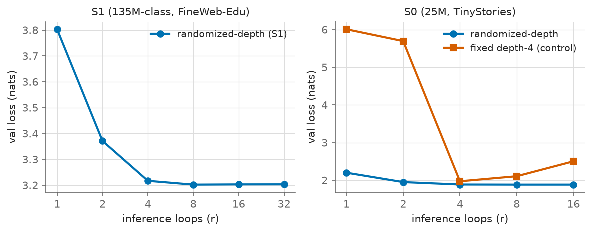
We first confirm that the backbone is depth-elastic, since the measurement and allocation results in the following subsections require it. This property is not a contribution of this work; it establishes the fixed model on which the rest is measured. Table 2 gives S1 validation loss as a function of inference loop count for the final checkpoint. Loss falls monotonically from 3.80 at one loop to 3.20 at eight, then stays flat: \(r=8\), 16, and 32 are 3.202, 3.203, and 3.203. The useful range spans a 16-fold difference in per-token compute (\(r=1\) versus \(r=16\)) with a 0.60-nat quality range across it, all from one set of weights chosen at inference time. Running four times deeper than the training mean does not degrade quality. The same shape held at every checkpoint we swept during training (Appendix 9), so it is a stable property of the model, not of a particular point in the schedule.
The fixed-depth control quantifies the contrast. A model trained at a constant four loops (S0) is sharply peaked at its training depth: loss 1.97 at \(r=4\) but 6.01 at \(r=1\) and 2.50 at \(r=16\). The randomized-depth model at the same scale is flat and low across \(r=4, 8, 16\) (1.886, 1.883, 1.883), and it is slightly better than the control even at the control’s own specialized depth. Randomized depth confers robustness that fixed depth does not, at no cost at the depth for which the fixed model was tuned.
5.2 Why saturation at the training mean↩︎
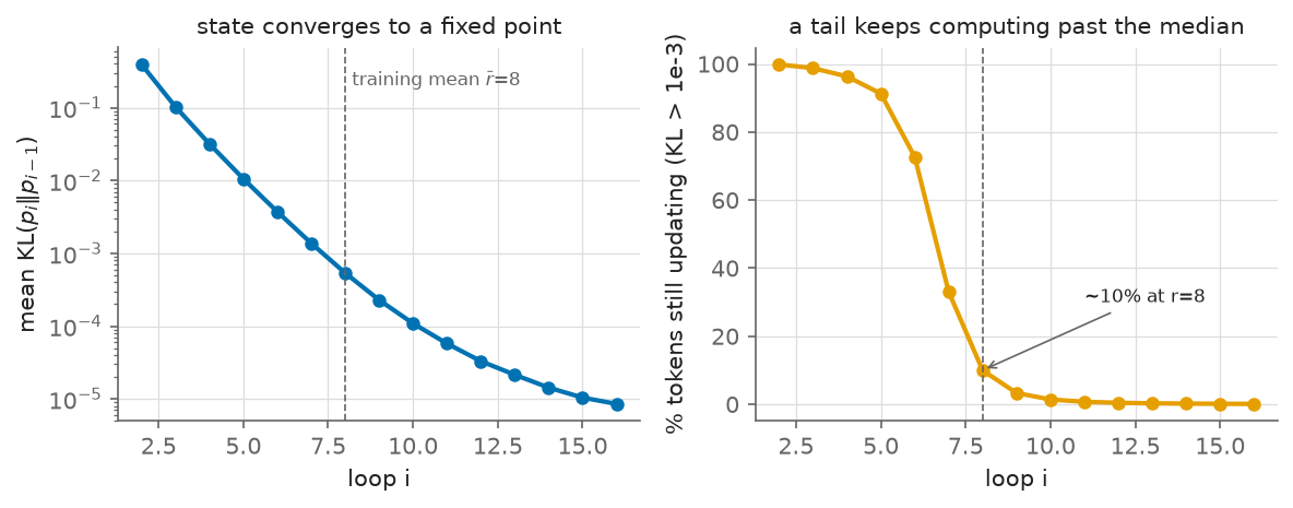
The flat region beyond \(r=8\) admits two readings: the loop could be spinning without effect, or the computation could be genuinely finished. These are distinguishable by measurement, and the distinction matters because the two readings imply different things about the architecture. Table 3 reports, per loop, the mean successive-output KL, the mean state change \(\|s_i - s_{i-1}\|\), and the fraction of tokens still moving (KL above \(10^{-3}\)). Both KL and state change decay smoothly toward zero together: KL is \(3.9\times10^{-1}\) at loop 2, \(5.4\times10^{-4}\) at loop 8, and \(8.5\times10^{-6}\) at loop 16. The state reaches a fixed point. Loss saturates at the training mean because the computation is finished there, not because the loop is broken. This is the behavior the architecture was designed for (noise initialization plus input re-injection push the core toward a contraction), and it explains why extrapolated depths are safe: iterating past convergence leaves a converged state where it is.
The decay is not uniform across tokens. At loop 7, 33 percent of tokens are still moving; at loop 8, 10 percent; by loop 16, 0.1 percent. The median token has converged by about loop 6, but a tail of roughly one token in ten needs the full training-mean depth. Uniform depth incurs the tail’s cost on every token. That tail is the allocation opportunity, and Section 5.3 is downstream of this measurement: we measured the tail first and then tested whether a policy could exploit it.
5.3 Allocation↩︎
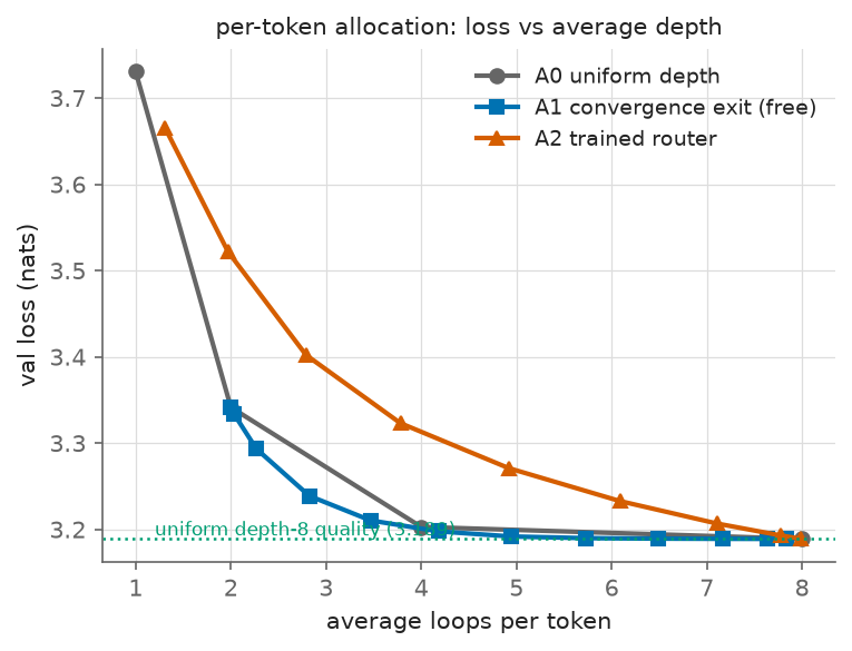
Table 4 gives loss at matched average depth for the three policies on the final model (128 windows). The uniform depth-8 quality bar is 3.189. The convergence exit A1 reaches that quality at 4.94 average loops, a 38 percent reduction in average depth, and it matches or exceeds uniform depth across the range. At average depth 3 the margin is clear (3.231 against 3.272); at average depths 4 through 7 the two are within 0.002 to 0.003 nats, with A1 never higher. At these evaluation sizes we claim that A1 matches uniform depth at matched average depth and outperforms it at the shallow end, without claiming strict dominance at every point. The mechanism is the one measured in Section 5.2: A1 halts the converged majority early and allocates the reclaimed loops to tokens whose state is still evolving.
The trained router A2 needs average depth 7.99 to reach the same quality, yielding no saving, and underperforms A1 across the range. This reproduces and strengthens the S0 result, in which A1 matched uniform depth and A2 underperformed. The explanation is direct: the convergence exit observes the model’s per-token state dynamics, whereas the probe predicts them from a single state snapshot and is a less accurate estimator of the same quantity. At S0 the two policies had little to separate them because the toy model’s useful-depth range was narrow; at S1 the wider range exposes the difference. A policy that must be trained, calibrated, and re-tuned per budget loses to a policy with zero parameters.
Average depth is a FLOP proxy, and we scope the efficiency result accordingly. In our teacher-forced masking harness, A1 and A2 loop every token to \(r_{\max}\) and mask the frozen ones, so they skip no work and realized throughput does not beat uniform depth. A matched-depth wall-clock timing (uniform \(r=8\) against uniform \(r=5\), the approximate A1 average) gives a 1.48 to 1.51 times speedup across batch sizes 1 to 8, which is the best case achievable if depth-wise batching packed exited tokens perfectly. The three-point bracket is therefore: 38 percent by average depth, about 1.5 times best-case wall-clock, and about 0 percent realized in our harness. Unlike layer-skip early exit, where a 3 times FLOP saving collapsed to single-digit wall-clock because the skips are ragged per-layer holes in a batch, the recursive saving is in whole forward passes of a shared-weight core, so exited tokens free schedulable work and the FLOP proxy and best-case wall-clock stay close. Closing the remaining gap is a systems problem (depth-wise continuous batching, demonstrated by [6]) that we did not build.
5.4 Token-level behavior↩︎
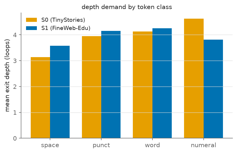
Depth demand tracks token type. Mean exit depth at S1 orders as space 3.58, numeral 3.81, punctuation 4.16, word 4.25. At S0 the order was space, punctuation, word, numeral, with numerals deepest. The ordering of the two content classes flips between scales. We attribute this to distribution shift: TinyStories contains simple recurring arithmetic that rewards depth on numerals, whereas FineWeb-Edu numerals are often rare isolated tokens the model cannot resolve further, and words carry the compositional load. The ordering was stable under a four-fold increase in evaluation windows, so it is a dataset effect, not sampling noise. The general pattern, structural tokens exiting early and content tokens computing longer, matches what the adaptive-depth literature has reported since ACT [8], here obtained without any learned halting.
5.5 Ceiling reference↩︎
Evaluated under our S1 harness, SmolLM2-135M scores 2.66 nats against the recursive model’s 3.20 at \(r=8\), a gap of 0.54 nats. This is a ceiling reference, not a matched baseline, for two reasons. First, SmolLM2-135M trained on roughly 2T tokens, about 150 times our budget, so a gap is expected from the token count alone. Second, SmolLM2 trained on FineWeb-Edu while our evaluation set is FineWeb-Edu validation, so plausible train-eval overlap inflates its score and widens the measured gap. Both effects widen the gap rather than narrow it.
5.6 The per-request cost curve↩︎
For the deployment framing, Table 5 restates the elasticity sweep as a cost curve: quality, measured tokens per second at batch 1 on one RTX 4090, and relative throughput at each uniform depth. From one checkpoint, an operator can serve depth 2 at 2.7 times the throughput of depth 8 for a 0.17-nat quality cost, or any point between, without a model switch or cache invalidation. These numbers are one GPU class and one implementation; they are included to make the product shape concrete, not as a serving benchmark.
6 Discussion and limitations↩︎
6.0.0.1 Useful depth is determined at training time.
Our hypothesis that useful depth would extend beyond the training mean at larger scale did not hold: the model saturates at the training-mean depth and gains nothing beyond it. Across our two scales the pattern is exact: trained at mean 4, saturates at 4; trained at mean 8, saturates at 8. Huginn, trained at mean 32, reports useful depth to 32 and beyond [2], which is consistent with the same rule. Two internal points and one external consistency check do not establish a law, and we have not tested a wider training distribution at fixed scale, so we state this as the paper’s main open hypothesis: a recursive model uses depth up to its training mean and no further. If it holds, it is a design lever: the saturation depth, and with it the width of the product’s quality-compute range, is chosen by the practitioner through the training loop distribution. The convergence measurement in Section 5.2 shows the model is not failing to use extra depth; it has finished computing.
6.0.0.2 Baselines and seeds.
We make no FLOP-matched parity claim. A matched vanilla transformer costs the same as the recursive run at iso-FLOP by construction, and there is no legitimate discounted version: a token-starved short vanilla would lose because it saw less data, not because it is architecturally worse, so we rejected that comparison. Parity is the natural next experiment, and the one on which any deployment argument most depends. S1 is a single seed. The S0 seed study has two of three seeds complete, with a maximum spread of 0.03 nats across the sweep and 0.011 nats at \(r=16\) between the two; we report this as observed and make no seed-variance claim.
6.0.0.3 Wall-clock.
Realizing the average-depth saving as throughput requires depth-wise continuous batching, as demonstrated by [6]. We did not build it, and we report the three-point bracket rather than an end-to-end speedup. We note that the structural situation is more favorable than for layer-skip early exit, for the reason given in Section 5.3, but a measured serving result is future work.
6.0.0.4 Scale.
All results are at 135M-class compute. The literature suggests the interesting depth effects strengthen with scale and task difficulty (Geiping et al. report reasoning-heavy tasks improving out to depth 64 while easy benchmarks saturate near 8), so our average-loss results on web text plausibly understate what per-token allocation offers on harder distributions. We have not tested this; behavior at 1B parameters and above is unknown.
6.0.0.5 What we did not solve.
The key-value cache story for per-token allocation at decode time is inherited from the recursion literature (per-recursion caching or depth-1 sharing [6]) and was not stress-tested here; our evaluation is teacher-forced. Downstream task evaluation at each depth, which would show whether reasoning-flavored capabilities track depth differently from average loss, was out of budget and remains open.
7 Conclusion↩︎
The recurrent state of a randomized-depth transformer converges to a per-token fixed point, and the depth at which it converges varies across tokens: the median token converges well before the training-mean depth while a minority continues to update at it. This variation is directly readable from the successive outputs, and reading it outperforms learning to predict it. A training-free convergence exit attains uniform depth-8 quality at 4.94 average loops and matches uniform depth across the average-depth range, with an advantage at shallow depths, whereas a router trained on labels from the same model requires close to full depth and provides no reduction. These allocation results hold at a single 135M-class scale on one seed, with average depth reported as a FLOP proxy rather than measured throughput and without a FLOP-matched dense baseline; the underlying convergence measurement is the more scale-independent finding. The depth elasticity on which all of this rests reproduces here from prior work rather than being contributed by it. Directions for future work are establishing the training-mean saturation pattern as a general property, converting the average-depth reduction into measured throughput under depth-wise batching, evaluating downstream capabilities as a function of depth, and testing whether the per-token convergence structure holds at larger scale. The complete study reproduces on a single RTX 4090 in approximately 100 GPU-hours.
Reproducibility statement↩︎
The training and evaluation code, configuration files, the experiment log, and the final S1 checkpoint are available at https://github.com/jlognn/depth-recurrent-convergence. Every number reported in this paper is recorded in the released log alongside the configuration and evaluation harness that produced it. The S1 model trains in approximately 100 GPU-hours on a single 24GB GPU.
8 Configuration↩︎
| S0 (toy) | S1 (main) | |
|---|---|---|
| Data | TinyStories | FineWeb-Edu |
| Tokens | 0.4B | 12.9B |
| \(d_{\text{model}}\) | 384 | 576 |
| Heads (KV heads) | 6 (2) | 9 (3) |
| FFN dim | 1024 | 1536 |
| Prelude / core / coda layers | 2 / 4 / 2 | 2 / 4 / 2 |
| Unique params (non-embedding) | 12.9M | 29.0M |
| Total params | 31.8M | 57.3M |
| \(\bar{r}\) (mean loops) | 4 | 8 |
| \(r_{\max}\) | 16 | 32 |
| Truncated-BPTT \(k\) | 4 | 8 |
| Sequence length | 512 | 2048 |
| Peak LR | \(1\times10^{-4}\) | \(1\times10^{-4}\) |
| Optimizer | AdamW (0.9, 0.95), wd 0.1 | AdamW (0.9, 0.95), wd 0.1 |
| Schedule | cosine, 1% warmup | cosine, 1% warmup |
| Seeds | 2 of 3 | 1 |
Full configuration JSONs ship with the code release.
9 Elasticity across training↩︎
| loops \(r\) | loss (nats) | ppl | tokens/s (batch 1) |
|---|---|---|---|
| 1 | 3.803 | 44.8 | 18336 |
| 2 | 3.371 | 29.1 | 12952 |
| 4 | 3.217 | 24.9 | 8186 |
| 8 | 3.202 | 24.6 | 4727 |
| 16 | 3.203 | 24.6 | 2577 |
| 32 | 3.203 | 24.6 | 871 |
Provisional sweeps at 12, 28, 76, and 91 percent of training showed the same monotone shape from the first checkpoint onward, with the whole curve descending as training progressed; the \(r=8\) to \(r=16\) gap never opened at any checkpoint. The S0 two-seed spread was at most 0.030 nats at any depth and 0.011 nats at \(r=16\).
10 Convergence and allocation tables↩︎
| loop \(i\) | mean KL | mean state change | percent tokens moving |
|---|---|---|---|
| 2 | \(3.9\times10^{-1}\) | 24.7 | 99.8 |
| 4 | \(3.2\times10^{-2}\) | 7.85 | 96.3 |
| 6 | \(3.7\times10^{-3}\) | 2.60 | 72.7 |
| 7 | \(1.4\times10^{-3}\) | 1.52 | 33.0 |
| 8 | \(5.4\times10^{-4}\) | 0.90 | 10.0 |
| 10 | \(1.1\times10^{-4}\) | 0.34 | 1.4 |
| 12 | \(3.3\times10^{-5}\) | 0.14 | 0.4 |
| 16 | \(8.5\times10^{-6}\) | 0.030 | 0.1 |
| avg depth | A0 uniform | A1 convergence exit | A2 trained router |
|---|---|---|---|
| 3 | 3.272 | 3.231 | 3.385 |
| 4 | 3.203 | 3.201 | 3.313 |
| 5 | 3.199 | 3.192 | 3.268 |
| 6 | 3.196 | 3.190 | 3.236 |
| 7 | 3.192 | 3.189 | 3.210 |
A1 reaches the depth-8 bar at 4.94 average loops (38 percent fewer); A2 needs 7.99.
| depth \(r\) | loss (nats) | tokens/s | relative throughput |
|---|---|---|---|
| 2 | 3.371 | 12952 | 2.7x |
| 4 | 3.217 | 8186 | 1.7x |
| 8 | 3.202 | 4727 | 1.0x |
| 16 | 3.203 | 2577 | 0.55x |
| 32 | 3.203 | 871 | 0.18x |
11 Training stability notes↩︎
Two numerical issues encountered during S1 bring-up are documented here because practitioners running mixed-precision training on this architecture are likely to encounter them.
11.0.0.1 Mixed-dtype attention.
Under bf16 autocast, the rotary embedding tables were built in fp32 (the embedding output dtype), and multiplying the bf16 query and key projections by fp32 tables promoted them to fp32 while the value projection remained bf16. Fused scaled-dot-product attention kernels reject mixed dtypes, and a broad exception handler in the training loop silently fell back to fp32 for the remainder of the run, so runs labeled bf16 could execute in fp32 without any visible error. The fix is one line, casting the rotary tables to the query dtype before application, plus removing the silent fallback so that dtype errors surface as errors. We recommend logging the observed dtypes of attention inputs once at the first step of any mixed-precision run.
11.0.0.2 Non-finite step guard.
The training loop skips the optimizer step when the loss or gradient norm is non-finite, logs every skip with its step number, and aborts if skips exceed 0.1 percent of steps or three consecutive occurrences. On a healthy configuration this guard never fires; treating any firing as a bug signal rather than noise to suppress was, in our experience, the correct policy.