1 Relevance↩︎

Point predictions are rarely the end goal of a signal processing pipeline, which ultimately needs to produce an action or a decision. For example, based on a prediction, a detector triggers an alarm, a scheduler assigns power or bandwidth, a controller selects a gain, a diagnostic system recommends a test. This lecture note explains, at a level accessible to a first-year graduate student, why good decisions require uncertainty quantification and which representation of uncertainty is appropriate for a given decision objective and state of knowledge. The material connects three topics that are usually taught separately, namely Bayesian decision theory, calibration of machine-learning predictors, and robust optimization, by placing them inside one decision problem and asking, for each, what statistic of the data is sufficient to act optimally.

2 Prerequisites↩︎

The reader is assumed to be comfortable with elementary probability (conditional distributions, expectation, Bayes’ rule), with the notion of an optimization problem and its optimal value, and with basic estimation. No prior exposure to conformal prediction, imprecise probability, or distributionally robust optimization is required. Familiarity with Bayesian inference at the level of an introductory machine-learning course [1] is helpful for the final section.

3 Problem Statement↩︎

We consider an agent that acts once in a given environment. The problem is described by the following random variables:

• a state \(s\in \mathcal{S}\) with distribution \(s\sim p(s)\);

• an observation \(o\in \mathcal{O}\) with conditional distribution \(p(o| s)\);

• an action \(a\in \mathcal{A}\) drawn from a policy \(\pi(a| o)\) as \(a \sim \pi(a| o)\);

• and a scalar utility, or reward, \(u(s,a)\), depending on state \(s\) and action \(a\).

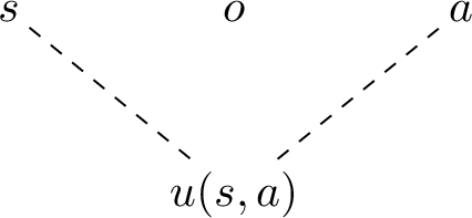
The joint distribution of the random variables \((s,o,a)\), taking values in sets \(\mathcal{S}\), \(\mathcal{O}\), and \(\mathcal{A}\), respectively, factorizes as \[\label{eq:joint} p(s,o,a)=\underbrace{p(s)\,p(o| s)\,}_{\text{environment }p(s,o)}\underbrace{\pi(a| o)}_{\text{policy}},\tag{1}\] with utility \(u(s,a)\). A graphical representation of the joint distribution, known as Bayesian network, is shown in Fig. 1. The agent controls the policy \(\pi(a| o)\), while the environment is described by the joint distribution \(p(s,o)=p(s)\,p(o| s)\), which dictates the state distribution \(p(s)\) and the observation model \(p(o|s)\). We assume throughout that the agent cannot modify the environment \(p(s,o)\) and has access only to the observation \(o\), and not to the underlying state \(s\), when selecting an action \(a\sim \pi(a|o)\).

The central question of this lecture note is: what must the agent know about the uncertain state \(s\), and in what form, in order to act optimally? As we will see, the answer depends both on the agent’s attitude toward risk and on whether the environment is known.

4 Solution↩︎

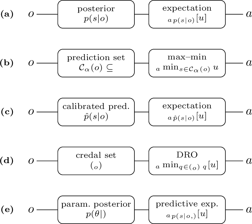
We build the answer in stages. Sections 4.1 and 4.2 treat a known environment and show how the decision objective (risk-neutral vs.risk-averse) dictates the form of uncertainty representation. Section 4.3 then confronts an unknown environment and introduces three complementary tools to address the resulting epistemic uncertainty. The five resulting settings are summarized in Fig. 2.

Throughout the text, we denote the distribution of a random variable \(x\in \mathcal{X}\) with support given by set \(\mathcal{X}\) as \(p(x)\), not differentiating between the value \(p(x)\) for a given numerical realization \(x\) and the entire function \(\{p(x)\}_{x\in \mathcal{X}}\). We also do not differentiate between random variable \(x\) and its realization, which is also denoted as \(x\). We use \(\mathbb{E}_{x\sim p(x)}[\cdot]\) and \(\Pr_{x\sim p(x)}[\cdot]\) for expectation and probability evaluated with respect to distribution \(p(x)\).

4.1 Known Environment, Risk-Neutral Agent: The Posterior as Interface↩︎

A risk-neutral agent optimizes the average utility, solving the problem \[\label{eq:opt1} \max_{\pi(a| o)}\;\mathbb{E}_{(s,o,a)\sim p(s,o)\pi(a| o)}\!\left[u(s,a)\right],\tag{2}\] where the utility \(u(s,a)\) is averaged over both the environment distribution \(p(s,o)\) and the policy \(\pi(a|o)\). By the law of iterated expectations, the optimization (2 ) decouples across observations, yielding the equivalent form \[\label{eq:inner} \mathbb{E}_{o\sim p(o)}\!\left[\max_{\pi(a| o)} \mathbb{E}_{a\sim \pi(a|o)}[U(a| o)]\right],\tag{3}\] where \[\label{eq:uoa} U(a| o)=\mathbb{E}_{s\sim p(s| o)}\!\left[u(s,a)\right]\tag{4}\] is the average utility of action \(a\) conditioned on the environment producing observation \(o\). The conditional state distribution used in the averaged utility (4 ) follows from Bayes’ rule as \[\label{eq:posterior} p(s| o)\propto p(s)\,p(o| s).\tag{5}\]

By the equivalent form (3 ), the agent can optimize its action separately for each observation \(o\) based on the conditional state distribution \(p(s|o)\). Furthermore, because the objective in the inner optimization in 3 is linear in the policy, the problem is solved by a deterministic policy choosing the action \[\label{eq:optaction} a^*(o)=\mathop{\mathrm{arg\,max}}_{a \in \mathcal{A}} U(a| o).\tag{6}\] An example of utility \(u(s,a)\), posterior \(p(s|o)\), and average utility \(U(a|o)\) is shown in Fig. 3.

The key result of this section is that the posterior distribution \(p(s| o)\) is a sufficient statistic of the observation \(o\) for the decision problem: an optimal agent need retain nothing about \(o\) or the environment beyond \(p(s| o)\). Equivalently, as summarized in Fig. 2 (a), the map \(o\mapsto p(s| o)\) is the optimal interface between the agent and its environment.

4.2 Risk-Averse Agent: Prediction Sets as Interface↩︎

Instead of the mean, an agent may value the utility it can guarantee with high probability over the unknown state \(s\sim p(s| o)\). Fix a risk level \(\alpha\in(0,1)\). For an observation \(o\) and action \(a\), the value-at-risk at level \(\alpha\) is \[\label{eq:var} V_\alpha(a| o)=\sup\Bigl\{\nu\in\mathbb{R}:\; \Pr_{s\sim p(s| o)}\!\left[\,u(s,a)\ge\nu\,\right]\ge 1-\alpha\Bigr\}.\tag{7}\] This is the largest utility attained with probability at least \(1-\alpha\) under the posterior, or, equivalently, the lower \(\alpha\)-quantile of the utility \(u(s,a)\). The risk-averse agent maximizes it by addressing the problem \[\label{eq:optactionalpha} a_\alpha^*(o)=\mathop{\mathrm{arg\,max}}_{a \in \mathcal{A}} V_\alpha(a| o).\tag{8}\] As \(\alpha\to0\) the objective concentrates on the worst outcomes, trading expected utility for protection against low-utility states.

As shown next, this quantile objective can be recast as a worst-case optimization over a prediction set, motivating a different interface between decision maker and environment – from a probability distribution to a set. To elaborate, let a level-\(\alpha\) prediction set be a map \(o\mapsto \mathcal{C}_{\alpha}(o)\subseteq\mathcal{S}\) satisfying the coverage guarantee \[\label{eq:coverage} \Pr_{s\sim p(s| o)}\!\left[\,s\in \mathcal{C}_{\alpha}(o)\,\right]\ge 1-\alpha.\tag{9}\] By (9 ), the set \(\mathcal{C}_{\alpha}(o)\) is guaranteed to contain the true state \(s\) with probability no smaller than \(1-\alpha\) given the observation \(o\). An example of a level-\(\alpha\) prediction set is shown in Fig. 3.

Given such a set, as also illustrated in Fig. 3, the max–min policy selects the action maximizing the worst-case utility within the set, \[\label{eq:maxmin} a_{\mathrm{mm}}(\mathcal{C}_{\alpha}(o))=\mathop{\mathrm{arg\,max}}_{a\in\mathcal{A}}\;\min_{s\in \mathcal{C}_{\alpha}(o)}u(s,a),\tag{10}\] with corresponding worst-case value \[\label{eq:umm} U_{\mathrm{mm}}(\mathcal{C}_{\alpha}(o))=\max_{a\in\mathcal{A}}\;\min_{s\in \mathcal{C}_{\alpha}(o)}u(s,a).\tag{11}\] As shown next, this worst-case value is an achievable value-at-risk for the max–min action.

Lemma 1 shows that any prediction set with a coverage guarantee yields, through the max–min rule, an action with a certified value-at-risk. The next proposition shows that the value-at-risk optimal action 8 is recovered by choosing the coverage set optimally, so that a max–min decision based on a suitably designed prediction set incurs no loss of optimality.

The results developed in this section show that a risk-averse agent can operate without loss of optimality on the basis of a prediction set \(\mathcal{C}_{\alpha}(o)\subseteq\mathcal{S}\) with coverage guarantees, acting by targeting the worst case over that set 10 . This is illustrated in Fig. 2 (b). In this regard, by Lemma 1, any set satisfying the coverage condition 9 yields a max–min action with the value-at-risk guarantee 12 . Moreover, an optimized set – namely \(C_\alpha^*(o)\) in ?? – yields the largest value-at-risk certificate, recovering the value-at-risk optimal action \(a_\alpha^*(o)\).

So far coverage 9 has been imposed conditionally, i.e., for each observation \(o\). One may instead require coverage on average over observations, \[\label{eq:margcoverage} \Pr_{(s,o)\sim p(s,o)}\!\left[\,s\in \mathcal{C}_{\alpha}(o)\,\right]\ge 1-\alpha,\tag{14}\] which is weaker than 9 . Prediction sets with the marginal guarantee 14 can be constructed by conformal prediction using only data, without knowledge of the environment [2], [3]. Reference [4] shows that results analogous to Lemma 1 and Proposition 1 hold when the value-at-risk objective 7 is replaced by a suitable average, placing conformal prediction on a decision-theoretic footing. The next sections address the setting with an unknown environment.

4.3 Unknown Environment: Three Routes to Uncertainty Quantification↩︎

Suppose now that the environment distributions \(p(s)\) and \(p(o| s)\) are unknown. We treat this setting in three ways, each highlighting a different approach to uncertainty quantification. For a preview of the main results, Fig. 2 (c)–(e) summarizes the resulting interfaces.

\(\bullet\) Fixed predictor. A predictor \(\hat{p}(s| o)\) is supplied to the agent. Under what conditions can the agent act on it, and trust that the resulting performance is as good as it can be given that the policy can be based solely on the predictor? The answer motivates calibration as a key property of predictors (Sec. 4.4).

\(\bullet\) Data-driven non-parametric predictor. No predictor is given, but a dataset \[\label{eq:dataset} \mathcal{D}=\{(o_i,s_i)\}_{i=1}^{n}\;\stackrel{\text{i.i.d.}}{\sim}\;p(s,o)=p(s)\,p(o| s)\tag{15}\] of \(n\) observation–state pairs is available. Because the dataset size \(n\) is finite, plugging a naive estimate into the known-environment solution is generally suboptimal, and the agent must account for the epistemic uncertainty caused by the availability of limited data. A non-parametric treatment of this uncertainty leads to credal sets and distributionally robust optimization (Sec. 4.5).

\(\bullet\) Data-driven parametric predictor. Under parametric assumptions, the same epistemic uncertainty can be optimally accounted for by Bayesian inference over model parameters (Sec. 4.6).

4.4 Unknown Environment I: Fixed Predictor and Calibration↩︎

Assume a fixed predictor \(\hat{p}(s| o)\), generally not equal to the true posterior \(p(s| o)\). Treating the predictor \(\hat{p}(s| o)\) as if it were the true posterior, the agent takes, in place of 6 , the action \[\label{eq:optaction1} a^*(\hat{p}(s| o))=\mathop{\mathrm{arg\,max}}_{a \in \mathcal{A}} \hat{U}(a| o),\tag{16}\] where the estimated utility under the predictor is \[\label{eq:uhat} \hat{U}(a| o)= \mathbb{E}_{s \sim \hat{p}(s| o)}[u(s,a)].\tag{17}\] When does this action guarantee some notion of optimality? As seen in this section, this is the case when the predictor is calibrated.

A predictor is distribution calibrated if, among all observations \(o\) that yield a given predictive distribution \(q(s)\), i.e. \(\hat{p}(s| o)=q(s)\), the true fraction of states equal to \(s\) equals the predicted value \(q(s)\). Formally, with \[\label{eq:Oq} \mathcal{O}_{q(s)}=\{o\in \mathcal{O}:\hat{p}(s'| o)=q(s')\;\text{for all }s'\in\mathcal{S}\}\tag{18}\] denoting the set of observations mapped to the predictive distribution \(q(s)\), a distribution-calibrated predictor satisfies \[\label{eq:distcal} p(s' | o\in\mathcal{O}_{q(s)})=q(s')\qquad \text{for all } s'\in\mathcal{S}.\tag{19}\] In words, a distribution-calibrated model provides predictive probabilities that reflect the true conditional state frequencies.

Unlike 6 , the optimality condition ?? involves an expectation over observations \(o\). The price of acting through a predictor, even a calibrated one, is that optimality is generally guaranteed only on average, not per observation. As Example 1 shows, this price can be steep: a calibrated predictor may be completely uninformative, so its action cannot adapt to the observation \(o\).

In practice, given a predictor, the level of miscalibration must be estimated from a finite validation set. Checking full distribution calibration 19 would require binning the space of predictive distributions, which is impractical beyond a few dimensions. The most common metric, namely the expected calibration error (ECE) [6], therefore restricts attention to the predicted probability of the most likely class. While intuitive, the ECE is a biased and inconsistent estimator: its value depends on the arbitrary number and width of the bins, and no binning scheme can simultaneously average away sampling noise and retain the resolution needed to localize miscalibration [7]. Binning-free alternatives instead plot the cumulative difference between predicted and observed outcomes, ordered by predicted probability, and come with rigorous \(p\)-values for the null hypothesis of perfect calibration, giving a consistent and reproducible assessment [7].

When a predictor is found miscalibrated, calibration can be partially restored by post-hoc methods such as temperature or Platt scaling, which fit a few parameters on held-out data to align predicted probabilities with observed frequencies [5], [6].

4.5 Unknown Environment II: Credal Sets and Robust Optimization↩︎

Consider now the case with no predictor given but a dataset 15 available. In this section, we take both variables \(s\) and \(o\) discrete, with finite cardinalities \(|\mathcal{S}|\) and \(|\mathcal{O}|\). A natural first step is to evaluate the histogram, the simplest non-parametric estimator of \(p(s| o)\). Define the sub-dataset \[\label{eq:subdataset} \mathcal{D}_o=\{(o_i,s_i)\in\mathcal{D}: o_i=o\}\tag{20}\] of the \(n_o=|\mathcal{D}_o|\) pairs with observation \(o\). The histogram is the vector of state frequencies \[\label{eq:emppost} \hat{p}^{\text{hist}}(s| o)=\frac{1}{n_o}\sum_{i:\,o_i=o}\mathbf{1}\{s_i=s\},\tag{21}\] where \(\mathbf{1}\{\cdot\}\) is the indicator function. The corresponding estimated utility 17 for a fixed action \(a\) is the empirical mean \[\label{eq:uhathist} \hat{U}(a|\mathcal{D}_o) = \frac{1}{n_o} \sum_{(o_i,s_i) \in \mathcal{D}_o} u(s_i,a).\tag{22}\]

This quantity is not a reliable performance certificate. To see why, conditioned on the dataset size \(n_o\), consider the out-of-sample disappointment [8] \[\label{eq:disappointment} \Pr_{\mathcal{D}_o\sim p(s| o)^{\otimes n_o}}\!\bigl[\,U(a| o) < \hat{U}(a|\mathcal{D}_o)\,\bigr],\tag{23}\] the probability that the true utility falls short of its data-driven estimate, over draws of the training data. The notation \(p(s| o)^{\otimes n_o}\) represents the product distribution of the i.i.d.dataset \(\mathcal{D}_o\). By the central limit theorem, this probability tends to \(1/2\) as \(n_o\) grows: the plug-in estimate is optimistic about half the time. Quantifying the uncertainty of \(\hat{p}(s| o)\) is therefore essential.

A principled remedy uses credal sets and distributionally robust optimization (DRO). Define a set of conditional distributions in a neighborhood of the empirical distribution as \[\label{eq:klball} \mathcal{P}(\mathcal{D}_o)=\bigl\{\,q(s):\;\mathrm D\!\left(q(s),\,\hat{p}^{\text{hist}}(s| o)\right)\le r\,\bigr\},\tag{24}\] where \(\mathrm D(\cdot,\cdot)\) is a divergence between distributions and \(r>0\) controls the set size. When the divergence measure \(\mathrm D\) is convex in its first argument – as for every \(f\)-divergence, including the Kullback–Leibler (KL) divergence and total variation (TV) distance – the set 24 is a credal set: a closed, convex set of probability distributions [9]. The agent then optimizes the worst-case utility over the set, solving the DRO problem \[\label{eq:mmaction} a_{\mathrm{mm}}(\mathcal{D}_o)=\arg\underbrace{\max_{a\in \mathcal{A}}\;\min_{q(s)\in \mathcal{P}(\mathcal{D}_o)} \mathbb{E}_{s\sim q(s)}[u(s,a)]}_{U_{\mathrm{mm}}(\mathcal{D}_o)}.\tag{25}\]

Suppose the divergence and radius are chosen so that the set covers the true posterior with probability at least \(1-\delta\), \[\label{eq:coveragedro} \Pr_{\mathcal{D}_o\sim p(s| o)^{\otimes n_o}}\!\bigl[\,p(s| o)\in\mathcal{P}(\mathcal{D}_o)\,\bigr]\ge 1-\delta.\tag{26}\] For example, with the TV distance \(\mathrm{TV}(q(s),q'(s))=\tfrac12\sum_{s\in\mathcal{S}}|q(s)-q'(s)|\) and radius \[\label{eq:radius} r=\sqrt{\frac{|\mathcal{S}|\log 2+\log(1/\delta)}{2\,n_o}},\tag{27}\] a finite-sample deviation bound for the empirical distribution [10] guarantees \(\mathrm{TV}(\hat{p}^{\text{hist}}(s| o),\,p(s| o))\le r\) with probability at least \(1-\delta\), so that the condition 26 holds.

The certificate \(U_{\mathrm{mm}}(\mathcal{D}_o)\) is thus a reliable high-confidence lower bound on the utility the data-driven action will actually achieve. With probability at least \(1-\delta\), the realized utility is no worse than the certified value, so the agent may safely plan against \(U_{\mathrm{mm}}(\mathcal{D}_o)\) rather than the optimistic empirical mean 22 . This DRO-based approach corresponds to the interface illustrated in Fig. 2 (d).

Credal sets satisfying 26 trade off conservatism against tightness: a larger set gives stronger coverage but a smaller, less useful certificate. Asking for the least conservative such rule – the pointwise largest certificate among all rules with controlled disappointment – singles out a specific design. Reference [11] shows that, in the large-sample regime, choosing the metric \(\mathrm D\) to be the KL divergence is optimal in this sense, yielding actions whose certificate exhibits disappointment decaying exponentially, as \(\exp(-n_o r)\), where \(r\) is the radius in (24 ).

4.6 Unknown Environment III: Bayesian Inference↩︎

Under parametric assumptions, the state–observation relationship is modeled by a family \(p(s| o,\theta)\) indexed by parameters \(\theta\in\Theta\), equipped with a prior \(p(\theta)\). Epistemic uncertainty now resides in the lack of knowledge about \(\theta\). Given the dataset 15 , Bayes’ rule yields the parameter posterior \[\label{eq:parampost} p(\theta|\mathcal{D})\propto p(\theta)\prod_{i=1}^{n} p(s_i| o_i,\theta),\tag{28}\] and the posterior predictive distribution of the state is obtained by marginalizing over it, \[\label{eq:predictive} p(s| o,\mathcal{D})=\mathbb{E}_{\theta \sim p(\theta|\mathcal{D})}\!\bigl[p(s| o,\theta)\bigr].\tag{29}\] Repeating the risk-neutral argument of Sec. 4.1 with the conditional distribution \(p(s| o)\) replaced by the predictive 29 , the optimal action is \[\label{eq:bayesact} \begin{align} \hat{a}(o)&=\mathop{\mathrm{arg\,max}}_{a}\;\mathbb{E}_{s \sim p(s| o,\mathcal{D})}[u(s,a)]\\ &=\mathop{\mathrm{arg\,max}}_{a}\;\mathbb{E}_{\theta \sim p(\theta|\mathcal{D})}\mathbb{E}_{s\sim p(s| o,\theta)}[u(s,a)]. \end{align}\tag{30}\]

Hence, optimal risk-neutral decision making requires the parameter posterior \(p(\theta|\mathcal{D})\), and the predictive posterior 29 plays exactly the role of the known-environment interface \(o\mapsto p(s| o)\), as illustrated in Fig. 2 (e). In this regard, it is worth noting that a plug-in estimate that replaces the posterior \(p(\theta|\mathcal{D})\) by a point estimate such as maximum-likelihood, and acts on the distribution \(p(s| o,\hat{\theta})\) would discard this epistemic uncertainty and is again prone to out-of-sample disappointment.

Since the normalizing constant in 28 is rarely tractable, one in practice resorts to approximate inference – the Laplace approximation, variational inference, or Markov chain Monte Carlo; see [1], [12].

5 What We Have Learned↩︎

The recurring lesson in these notes is that a reliable decision needs an uncertainty representation matched to its objective, and a guarantee that certifies the value actually obtained.

• In a known environment, a risk-neutral agent needs only the posterior \(p(s| o)\) and maximizes expected utility; a risk-averse agent needs a prediction set and maximizes worst-case utility. Coverage of the set certifies a value-at-risk (Lemma 1), and the optimally chosen set comes with no loss of optimality (Proposition 1).

• With a fixed predictor, distribution calibration makes the plug-in action optimal – but only on average over observations (Proposition 2). Calibration is neither accuracy nor informativeness (Example 1), and measuring it reliably calls for binning-free, statistically consistent metrics.

• With finite data, the empirical mean is an optimistic, and hence untrustworthy, criterion causing out-of-sample disappointment. A credal set that covers the truth with high probability turns the max–min value into a high-confidence certificate (Proposition 3); and the KL-based rule is asymptotically the least conservative such choice.

• Under parametric models, the parameter posterior is the sufficient statistic, and the posterior predictive plays the role of the known-environment interface. Point estimates discard this uncertainty and reintroduce disappointment.

Calibration, conformal prediction, credal sets and DRO, as well as Bayesian inference are usually presented as separate topics. Seen through a single decision problem, they are complementary answers to one question – what is a sufficient, trustworthy summary of uncertainty for the decision at hand? – and together they make the case that decision making needs uncertainty quantification.

Author↩︎

Osvaldo Simeone (o.simeone@nulondon.ac.uk) is the Professor of Information Engineering at Northeastern University London, where he co-directs the Institute for Intelligent Networked Systems (INSI), and a visiting Professor at Aalborg University. Prof. Simeone is the author of the textbooks "Machine Learning for Engineers" and "Classical and Quantum Information Theory" published by Cambridge University Press, four monographs, two edited books, and more than 250 research journal and magazine papers. He is a Fellow of the IET and IEEE.

References↩︎