Logical Foundations of Two-Sided Type Theory
July 15, 2026
Abstract
Two-sided type systems, introduced in POPL’24, are an extension of the traditional notion of type system that allows for stating and deriving typing judgements in which (a) assumptions can be made about the types of arbitrary terms and not only variables, and (b) conclusions can be made about any number of type assignments, and not exactly one. In this work, we investigate the logical foundations of two-sided type systems in the sense of the propositions-as-types paradigm. We introduce new two-sided type systems and that correspond with Wansing’s bilateral logic and its extension with Nelson’s strong negation respectively. Going beyond the propositional case, we introduce as an extension of Guevers’ , and we show its expressive adequacy, its consistency and that it satisfies both the existence property and its dual.
1 Introduction↩︎
Two-sided type systems are a generalisation of the usual conception of type system, designed to allow the refutation as well as the verification of type assignments [1], [2]. A two-sided typing judgement generally has shape \(M_1:A_1,\,\ldots,\,M_k:A_k \types N_1:B_1,\,\ldots,\,N_m:B_m\) in which all the \(M_i\) and \(N_j\) are arbitrary terms. So, in a two-sided judgement: (i) one may make assumptions about the types of a compound expression \(M_i:A_i\), not necessarily a variable, and (ii) one may conclude any number of typings \(N_j:B_j\), not only a singleton. The meaning of such a judgement smoothly generalises that of a traditional judgement, namely: if all of the \(M_i\) each evaluates to a value of type \(A_i\) then some \(N_j\) will evaluate to a value of type \(B_j\) (or diverge).
This generalisation opens up interesting possibilities for the kinds of properties that can be reasoned about using type assignment. The following example is taken from [1]. Consider a typical definition of addition over natural number numerals in a simple PCF-like functional language: \[\abbv{add} \mathrel{\vcenter{:}}= \fixtm{f(x,y)}{\ifztm{y}{x}{\succtm\,(f\,(x,\predtm\,y))}}\] In the two-sided system of loc cit, as usual one can show that, whenever the inputs \(x\) and \(y\) are numerals, then their addition will also evaluate to a numeral: \[x:\natty,\,y:\natty \types \abbv{add}\,(x,y) : \natty\] However, one may also use the freedom of the two-sided judgement to show that, whenever the addition of \(x\) and \(y\) evaluates to a numeral, then \(x\) and \(y\) must have been numerals: \[\abbv{add}\,(x,y) : \natty \types x : \natty \qquad \abbv{add}\,(x,y) : \natty \types y : \natty\]
When discussing informally the behaviour of this program, it is quite natural to state that \(\abbv{add}\,(x,(\abs{y}{y}))\) will not evaluate to a numeral, but this is not something that can typically be made precise in a traditional type system. However, using the freedom to conclude any number of type assignments allows for this statement to be formalised in the two-sided system: \[\abbv{add}\,(x,(\abs{y}{y})) : \natty \types\] That is, for any \(x\), if \(\abbv{add}\,(x,(\abs{y}{y}))\) evaluates to a numeral then absurdity follows. Thus, a typing derivation rooted at this judgement constitutes a certificate of the defectiveness of the program \(\abbv{add}\,(x,(\abs{y}{y}))\). The subsequent work of [2] develops a more feature-full system that certifies the defectiveness of textbook examples of Erlang-like programs.
![Figure 1: Rules of the two-sided systems for pure \lambda-terms from [1], [2].](/article/2607.14325/_pdflatex/lzsyonua.png "fig:")
1.0.0.1 Rules of Two-Sided Systems
We represent on the left-hand side of Figure 1 the simple set of core rules for pure \(\lambda\)-terms that was identified in [1] and refined in [2]. On the right-hand side we enumerate the complementation rules that were the principal subject of [2]1. The idea is that the rules , and describe how to prove a typing of a specific term shape on the right-hand side of the judgement, as usual, and the rules , and describe how to refute a typing of a specific term shape that occurs on the left-hand side of the judgement.
A key component is the type \(B \cotofun A\). To understand this type, it is instructive to first introduce the type \(B \coto A\), which is the type of those functions \(f\) that satisfy the following property: for all inputs \(x\), if \(f\,x\) evaluates to a value of type \(A\), then \(x\) was necessarily a value of type \(B\). Then the type \(B \cotofun A\) is the complement of this type, i.e. it describes those terms that do not behave according to \(B \coto A\). Hence, to refute that some term \(\abs{x}{M}\) behaves in accordance with \(B \cotofun A\) is to prove that it behaves in accordance with \(B \coto A\), that is: to demonstrate that whenever it returns an \(A\), then its argument must have been a \(B\). This is exactly the content of the rule. Conversely, when refuting that an arbitrary application \(M\,N\) evaluates to a value of type \(A\), it suffices to show that \(M\) is a function that, to return an \(A\) necessitates an argument that is a \(B\), and then to refute that \(N\) is a \(B\). This is exactly the content of the rule.
1.0.0.2 Propositions-as-Types
Although the natural symmetry of the rules is appealing, and (when extended with appropriate rules for typing constants) one can use them to prove and refute interesting properties of program expressions quite effectively, one is very quickly led to a natural question regarding their logical content in the propositions-as-types sense. Thus, in this work, we aim to answer the question is there a sense in which two-sided type systems correspond to logics?
On the face of it, the situation is unclear. Two-sided systems were introduced as a kind of sequent calculi for typing formulas \(M:A\) and it seems incorrect to view them as a description for the assignment of terms to sequent calculi for propositional formulas \(A\), since, for example, the term \(M\,N\) in the conclusion of is an elimination form.
If we consider only derivations using rules , and of Figure 1, then there is a clear correspondence with constructive proofs in minimal propositional logic. So, we might expect that derivations using the rules , and correspond to some kind of constructive refutations in minimal propositional logic. However, the complementation rules , , , and are left unaccounted for. Together they allow for a kind of double-negation elimination, since one may use them to prove \(\types \abs{x}{x} : (A^c)^c \to A\) for any type \(A\). Double-negation elimination is notoriously non-constructive, but the situation here is more nuanced. Although introducing or eliminating a complement typing formula \(M:A^c\) behaves like a negation in switching between the sides of the sequent, if we consider only the propositional formula \(A^c\), it does not behave like the logical negation of \(A\), for example, there is no sense in which its inhabitants amount to functions from \(A\) to the empty type.
Of course, just as not every (traditional) type system corresponds to a logic, we would not expect every two-sided type system to correspond to a logic either. In what follows we will show that, by restricting the kinds of typing rules and judgements that we consider, we can build a two-sided type system in which derivations \(\,\types M:A\) correspond to constructive proofs and derivations \(M:A \types\,\) correspond to constructive refutations, even in the presence of complementation. The logical side of the correspondence is Heinrich Wansing’s bilateral propositional logic [3], whose proof system consists of mutually inductive proof and dual proof (refutation) judgements. To incorporate the complementation rules, we look to David Nelson’s seminal 1949 work on Constructible Falsity [4], which introduced the strong negation, \(\sneg{A}\), as a means to repair the asymmetry between verification and falsification in intuitionistic logic. A constructive proof of the strong negation of \(A\) amounts to a constructive refutation of \(A\), and a constructive refutation of the strong negation of \(A\) amounts to a constructive proof of \(A\). Thus, the provability of \(\sneg{(\sneg{A})} \to A\) does not imply collapse.
Moreover, we show that the underlying ideas extend beyond the propositional case by introducing a two-sided extension of Geuvers’ [5], which is a type system that corresponds to a version of Church’s Simple Type Theory [6]. We show that, as one might expect of a constructive logic, for any appropriate context \(\Gamma\), our system enjoys the existence property:
: If \(\Gamma \types M : \SigmaType{a}{K}{A}\) then there are \(B\), \(N\) such that \(\Gamma \types B : K\) and \(\Gamma \types N : A[B/a]\).
Moreover, its bilateral nature, mediated by the strong negation, ensures it also satisfies the dual property. Namely, in any appropriate context \(\Gamma\), a refutation of \(\PiType{a}{K}{A}\) yields directly a construction \(B\) and a refutation of \(A[B/a]\).
: If \(\Gamma;\, M:\PiType{a}{K}{A} \types\,\) then there are \(B\), \(N\) such that \(\Gamma \types B : K\) and \(\Gamma;\,N : A[B/a] \types\)
In many cases of interest in computer science, this construction associated with the dual existence property is of inherent interest. For example, suppose we define reachability on a rooted, directed graph with edge relation \(E\) and root \(I\) by the usual second order formula: \[\abbv{Reachable}_{I,E} \mathrel{\vcenter{:}}= \tyabs{y}{\mathsf{node}}{\PiType{z}{\mathsf{node} \to \starsort}{z\,I \wedge (\PiType{uv}{\mathsf{node}}{z\,u \wedge E\,u\,v \to z\,v}) \to z\,y}}\] Then a refutation of this property \(\sneg{(\abbv{Reachable}_{I,E}\,J)}\) for some target node \(J\) yields, via the Dual Existence property, the construction of a set of nodes that both contains the root and is closed under the edge relation, and which nevertheless excludes \(J\): i.e. an inductive invariant.
1.0.0.3 Contributions.
In this paper we establish an understanding of two-sided type systems in terms of proof and refutation in systems of constructive logic.
I. We identify the dual notions of constructive proof and refutation (dual proof) in Wansing’s bilateral logic [3], and Nelson’s strong negation [4], as the logical counterparts of the two-sided typing judgements and the complementation operator, respectively.
II. We introduce new two-sided type systems and which extend the core rules of Figure 1 to encompass a rich set of logical operators.
(a) We show that derivability in our system and provability in
    Wansing's system correspond precisely
    (Theorem [1](#thm:wansing-equivalence){reference-type="ref"
    reference="thm:wansing-equivalence"}).

(b) We show that derivability in our system and provability in an
    extension of Wansing's system with strong negation correspond
    precisely
    (Corollary [1](#thm:wansing-equivalence-sneg){reference-type="ref"
    reference="thm:wansing-equivalence-sneg"}).
III. We introduce a new two-sided system as an extension of Geuvers’ , which is itself a system corresponding to Church’s Simple Type Theory.
 (a) Due to the bilateral nature of types in our system, the usual
     encoding of logical operators using higher-order quantification
     is insufficient. We give a new encoding that accounts for the
     dual nature of each operator, and show that is therefore, in a
     certain sense, expressively adequate
     (Theorem [2](#thm:hol2-expr-adequacy){reference-type="ref"
     reference="thm:hol2-expr-adequacy"}).

 (b) By introducing a mapping from to , we show that our system is
     strongly normalising
     (Theorem [4](#thm:hol2-sn){reference-type="ref"
     reference="thm:hol2-sn"}), consistent
     (Theorem [3](#thm:hol2-consistency){reference-type="ref"
     reference="thm:hol2-consistency"}), and satisfies both the
     existence and dual existence properties
     (Theorem [6](#thm:hol2-existence){reference-type="ref"
     reference="thm:hol2-existence"}).
1.0.0.4 Notation.
In the rest of this paper, since we only construct two-sided type systems for the proof theory of logics, we will leave behind the notation for types used in [1], [2] and seen in Figure 1. For simplicity, we will instead adopt notation that is closer to that for formulas. So, we will use \(\sneg{A}\) in preference to \(A^c\) for type corresponding to the strong negation of \(A\), and we will use \(A \coto B\) in preference to \(A \cotofun B\) for the type corresponding to \(A\) coimplies \(B\)2.
1.0.0.5 Structure
The rest of the paper is structured as follows. In Section 2, we introduce the ideas of strong negation and bilateral logics. In Section 3 we define our two-sided type systems and and show their correspondence with and . In Section 4 we define our two-sided system and, in Section 5 we demonstrate its expressive power. In Section 6 we prove consistency and in Section 7 we prove the existence property and give some examples of its use in practice. Finally, in Section 8 we conclude and discuss related work.
2 Constructible Refutation, Strong Negation and Bilateralism↩︎
Intuitionistic logic is centred on proof. A proposition is explained by the constructions that count as its proofs, and the logical connectives are read as instructions specifying the form of evidence that must be supplied. For example, to prove \(A \wedge B\) is to give both a proof of \(A\) and a proof of \(B\); to prove \(A \vee B\) is to choose one of the two disjuncts and give a proof of it; and to prove \(A \to B\) is to give a construction which transforms any proof of \(A\) into a proof of \(B\).
One important consequence of this constructive meaning of proof is that intuitionistic logic satisfies the disjunction property:
if we have a proof of \(A \vee B\), then either we have
a proof of \(A\), or we we have a proof of \(B\)
In other words, a proof of a disjunction is not only evidence that one of the disjuncts holds, but contains enough computational information to recover which disjunct has been established.
If refutation is to be understood constructively in the same sense, then one might expect an analogous principle. That said, a refutation of a conjunction should not only rule out the conjunction as a whole; it should identify where the conjunction fails. This suggests the following property3:
if we have a refutation of \(A \wedge B\), then either we have
a refutation of \(A\), or we we have a refutation of \(B\)
However, this property is not validated by ordinary intuitionistic logic. The reason is that intuitionistic logic has no primitive treatment of refutation. Rather, refuting \(A\) is handled only indirectly, as proving its intuitionistic negation: \(\neg A \;:=\; A \to \bot\). The proposed principle of constructible refutation is then read intuitionistically as the following: \[\text{if } \vdash \neg(A \wedge B), \text{ then either } \vdash \neg A \text{ or } \vdash \neg B\] This statement is not valid, however. To see this, let \(A\) be a propositional variable and take \(B\) to be \(\neg A\). Intuitionistic logic proves \(\vdash \neg(A \wedge \neg A)\), since a proof of \(A \wedge \neg A\) immediately yields a contradiction, but it proves neither \(\neg A\) nor \(\neg\neg A\). Thus we have a intuitionistic refutation of \(A \wedge \neg A\), despite not having a intuitionistic refutation of either conjunct.
This failure isolates the difference between the construction of an intuitionistic refutation and a genuinely constructive account of refutation. To make the distinction even clearer, we quote the discussion from [8] (also highlighted in [3]), that separates the standard way of refuting a compound sentence, from the obvious rules for the refutation of a sentence. He describes the standard method as follows (terminology slightly adjusted to align with ours):
The standard way of refuting a compound sentence A is of course to make a series of inferences from the assumption that \(A\) holds that finally ends in the assertion (under the assumption \(A\)) of a contradiction ….
We see this in the intuitionistic notion of refutation, where \(\neg(A \wedge B)\) expresses that there cannot be any proof of \(A \wedge B\), but it does not by itself witness an actual failure that lies in \(A\) or lies in \(B\). Prawitz contrasts this with what he calls the obvious rules for the refutation of a sentence:
There are obvious rules for the refutation of a sentence such as inferring a refutation of \((A \wedge B)\) from a refutation of either \(A\) or \(B\), a refutation of \(A \vee B\) from refutations of both \(A\) and \(B\), a refutation of \(A \to B\) from a proof of \(A\) and a refutation of \(B\) and so on.
These rules characterize a genuinely constructive account of refutation. Under this approach, just as proofs are built connective by connective, refutations are also built by rules determined by the structure of the formula being refuted. This way, refutation is a primitive kind of evidence in its own right just like proof, in which sense they enjoy a equivalent status of proof in the system.
Conceptually, the idea of a more symmetric perspective on proof and refutation is quite natural. Proof is evidence for truth, while refutation is evidence for falsity; together, they form two sides of the same balance.
At the atomic level, both proof and refutation often arise from the same kind of basic act. For example, to verify or refute that a lemon is red, we just look at it. Here, both proof and refutation consists of an single visual experiment (with some meta-analysis of the result). In such cases, neither construction proceeds by assuming the opposite claim and deriving absurdity.
Moreover, it is natural that evidence of different kinds can combine to form more complex evidence. This is already visible in Prawitz’s obvious rules: to refute \(A \to B\), one supplies positive evidence for \(A\) together with negative evidence against \(B\). Thus, the construction of refutations cannot be described in isolation from the construction of proofs. A constructive account of refutation therefore calls for a framework in which proof and refutation coexist.
2.0.0.1 Towards constructivity for both proof and refutation
In what follows, we consider two systems that give primitive constructive content to both proof and refutation. The first is Nelson’s family of logics for constructible falsity, which begins with a primitive connective of strong negation. This connective functions as an object-language operation relating evidence for truth to evidence for falsity. The second is Wansing’s system , which has its roots in a more proof-theoretic standpoint. It treats proof and refutation as primitive, mutually related forms of bilateral judgement, thereby providing a different route to a constructive theory of refutation.
2.1 Nelson’s constructible falsity and strong negation↩︎
Nelson extends Kleene’s realizability [9] from truth to both truth and falsity. He observes that, from the viewpoint of constructibility, there are two distinct methods to falsify a formula. Consider, for example, a universal statement \(\forall x\,Q(x)\). One way to falsify it is to give an effective counterexample: a particular witness \(n\) together with evidence that \(Q(n)\) is false. Another way is to demonstrate that \(\forall x.Q(x)\) implies an absurdity. Nelson calls the former notion constructible falsity.4 To formalize this idea, he introduces two realizability relations: \[\begin{align} a \text{ P-realizes } A & \quad\text{means}\quad a \text{ encodes constructive evidence for the truth of } A, \\ a \text{ N-realizes } A & \quad\text{means}\quad a \text{ encodes constructive evidence for the falsity of } A . \end{align}\] The clauses for \(P\)-realizability and \(N\)-realizability are then defined simultaneously, by induction on the structure of formulas. In particular, Nelson introduces a primitive strong negation connective, which we will write \(\sneg{}\), to internalize constructible falsity: the constructible truth of \(\sneg{A}\) is identified with the constructible falsity of \(A\). It is interpreted by a switch between \(P/N\)-realizability: \[\begin{array}{l@{\qquad}l@{\quad}c@{\quad}l} (\sneg{P}) & a \text{ P-realizes } \sneg{A} & \text{iff} & a \text{ N-realizes } A, \\ (\sneg{N}) & a \text{ N-realizes } \sneg{A} & \text{iff} & a \text{ P-realizes } A . \end{array}\] This switchability is the key for \(\sneg{}\) being constructible. To P-realize \(\sneg{(\forall x\,Q(x))}\) is, by the clause \((\sneg{P})\), to N-realize \(\forall x\,Q(x)\). But Nelson’s clause for N-realizing \(\forall x\,Q(x)\) requires exactly a witness \(n\) together with an N-realizer of \(Q(n)\). Using \((\sneg{P})\) again, such an N-realizer of \(Q(n)\) is precisely a P-realizer of \(\sneg{Q(n)}\). Thus, the evidence of \(\sneg{(\forall x\,Q(x))}\) contains a witness \(n\) together with evidence of \(\sneg{Q(n)}\). In this sense, the falsification internalized by \(\sneg{}\) is genuinely constructible.
Nelson showed that his logic is conservative over an intuitionistic system of arithmetic, and he set out a Hilbert-style calculus, in which the behaviour of the strong negation is axiomatised through a number of equivalences:
Figure 2: 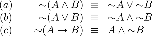 .
.
Figure 3: 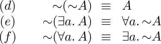 .
.
2.2 Wansing’s system↩︎
In [3], Wansing introduces the system , a bilateral5 natural-deduction system designed to combine both constructive proof and refutation, where refutation is understood as the dual of proof. The guiding idea is as follows: we start with the ordinary natural-deduction rules for intuitionistic proof; then read these rules from the opposite, falsificationist side; and finally add the mixed rules needed to let proof and refutation interact in a single calculus.
2.2.0.1 Two primitive kinds of derivation
The resulting system has two primitive kinds of derivation. A derivation of the first kind, called proof, gives constructive support for truth; a derivation of the second kind, called dual proof, gives constructive support for falsity. We write:
\(\wanp{\Pi,\,A,\,(L;R)}\), to mean that \(\Pi\) is a proof of \(A\) relative to the bilateral basis \((L;R)\);
\(\wandp{\Pi,\,A,\,(L;R)}\), to mean that \(\Pi\) is a dual proof, or refutation, of \(A\) relative to \((L;R)\)
Here \(L\) is a finite set of assumptions, whose formulas are treated as true, and \(R\) is a finite set of co-assumptions, whose formulas are treated as false. In particular, \(A\) is considered as a proof of \(A\) from the pair \(({A};\varnothing)\) and \(\overline{A}\) as a dual proof of \(A\) from the pair \((\varnothing;{A})\). Moreover, proofs may contain dual proofs as proper parts and dual proofs may contain proofs as proper parts.
For convenience, a full definition of , which encompasses all the usual propositional connectives, is given in For each propositional connective there are deduction rules for introducing it into a proof and deduction rules for introducing it into a dual proof. Similarly, there are deduction rules for eliminating it from a proof, and deduction rules for eliminating it from a dual proof. We mention here four that foreshadow the correspondence with two-sided type systems:
In this tree format, an inference ending with a formula under a single line represents a proof, and an inference ending with a formula under a double line represents a dual proof. Assumptions are discharged by writing them in single square brackets, and co-assumptions are discharged by writing them in double square brackets. The rules are, from left-to-right: implication introduction (proof), implication elimination (proof), coimplication introduction (dual proof), and coimplication elimination (dual proof).
The two proof rules are quite standard. The first of the dual proof rules says that to construct a dual proof of \(A \coto B\), one can construct a dual proof of \(B\) in which one can discharge the co-assumption \(A\). The second of the dual proof rules says that one can construct a dual proof of \(B\) from a dual proof of \(A \coto B\) and a dual proof of \(A\). Thus, just as implication internalises the notion of deduction for proofs, coimplication internalises the notion of deduction for dual proofs.
We draw the reader’s attention to the structural similarity of the above proof and dual proof rules with the typing rules on the left-hand side of Figure 1. Aside from the absence of terms, the Gentzen-style natural deduction format, and the alternative notation for coimplication; the rules above and the rules , , , and clearly correspond. Extrapolating from this observation, in the following section we will develop a two-sided type system that corresponds, in a precise sense, to .
3 A Language with Two-Sided Type System↩︎
None
Figure 4: \(\tintty{}\): Refutation Rules..
We now introduce , a term language equipped with a propositional two-sided type system corresponding to Wansing’s logic , and , its extension with Nelson-style strong negation. The design of the language follows the central idea of : proofs and refutations are treated uniformly as forms of evidence. Thus, terms are capable to express both proof and refutation.
Definition 1 (Types and Terms of ). Assume a denumerable set of term variables \(x,y,z\). The types* of the system, typically \(A, B,C\); and terms of the system, typically \(M,N,P\), are generated by the following grammars (usual conventions for bound variables are assumed): \[\begin{array}{rrcl} \rlnm{Types} & A,B,C & \Coloneqq & \falsefm \mid \truefm \mid A \wedge B \mid A \vee B \mid A \to B \mid B \coto A \\[0.4em] \rlnm{Terms} & M,N,P & \Coloneqq & x \mid \unittm \mid \abort(M) \mid (M,N) \mid \pi_1(M) \mid \pi_2(M) \\[0.2em] & & \mid & \inj_1(M) \mid \inj_2(M) \mid \casetm{M}{N}{P} \\[0.2em] & & \mid & \abs{x}{M} \mid M\,N \mid M\cdot{}N \mid \iota_1(M) \mid \iota_2(M) \end{array}\]*
The types of are the formulae of . The types \(\falsefm\) and \(\truefm\) are types for truth and falsity. \(A \wedge B\), \(A \vee B\) and \(A \to B\) are the standard sum, product and arrow types that relates to the connectives \(\wedge\), \(\vee\) and \(\to\) in intuitionistic logic. In addition, we have the type \(A \coto B\), pronounced \(A\) ‘coto’ \(B\). This corresponds to the coimplication connective \(\coto\) in 6. As the name suggests, this is supposed to be the dual of the implication connective \(\to\).
The terms are the evidence objects manipulated by the type system. A variable \(x\) names an available piece of evidence. The constant \(\unittm\) is nullary evidence, while \(\abort(M)\) is the eliminator associated with impossible evidence. The construction \(M\cdot{}N\) packages a pair of opposite evidence \(M\) and \(N\). Correspondingly, \(\iota_1\) and \(\iota_2\) are eliminators for mixed evidence \(M\cdot N\), where \(\iota_1\) extracts the first component \(M\), and \(\iota_2\) extracts the second component \(N\). The other forms are quite standard.
Definition 2 (Type contexts of ). A type context* is a finite set of typing formulae. Type contexts are usually denoted by \(\Gamma,\,\Delta,\,\Sigma,\,\Pi\), and written comma-separated: \(\Gamma = M_1:A_1,\dots,M_n:A_n\). Since contexts are finite sets, the order of the displayed formulae is irrelevant, and repeated occurrences of the same typing formula are ignored. Thus, whenever a context is displayed as above, we assume that the typing formulae \(M_1:A_1,\dots,M_n:A_n\) are pairwise distinct.*
Definition 3 (Type assignment for ). A typing judgement* is a pair of type contexts, written \(\Gamma \types \Delta\). A typing judgement is said to be provable, or derivable in \(\tintty\), if it can be obtained from the rules in 4 5 and the identity rule: \[\infer{ }{\Gamma,\,x:A \types x:A,\,\Delta}\;\mathrm{\small Id}\] Excepting this one, the conclusion of each rule distinguishes a single typing, which is called the principal formula of the rule.*
None
Figure 5: \(\tintty{}\): Proof Rules..
None
Figure 6: \(\tintcty{}\): Negation Rules..
The rules in 4 are the rules used for constructing the refutation of a formula. Rule says that falsity \(0\) requires a token refutation \(\abra{}\). Rule says that \(\abort(M)\) can be used as a refutation of any formula \(A\) whenever one has \(M\), a refutation of truth. Rule explains that a refutation of \(A \vee B\) consists of a pair, consisting of a refutation of \(A\) and a refutation of \(B\). Rule explains how to recover those refutations separately. The rules for conjunction are dual. Rule explains that a refutation of \(A \to B\) consists of a proof of \(A\) and a refutation of \(B\), which are put together in a package \(M \cdot{} N\), and explains how one may obtain the refutation \(N\) in the second component using \(\iota_2\) (the complementary rule explains how to obtain the proof component, but this is in Figure 5 because it constructs a proof). Finally, the rule constructs a refutation of a coimplication. A refutation of \(A \coto B\) expresses ‘if \(A\) is refutable then so is \(B\)’ and so the evidence consists of a function that assigns, to every refutation \(y\) of \(A\), a refutation \(M\) of \(B\). Such a function can be applied to a particular refutation \(N\) of \(A\) using the rule.
The rules in 5 are largely the usual rules for proving type assignments, excepting that now there is an additional context \(\Delta\) on the right-hand side which accounts for the fact that there may be further typing formulas on the right as well as on the left. The rule assigns \(M \cdot{} N\) the type \(A \coto B\): given the meaning of a refutation of \(A \coto B\) above, a proof should demonstrate that there is a refutation of \(A\) and yet a proof of \(B\). These opposing forms of evidence are packaged up in the dot construction, and explains how one can extract the proof using \(\iota_2\).
Definition 4 (). The system extends with strong negation. The terms of are the same as those of , while its types are obtained by adding the type former \(\sneg A\). Type contexts and typing judgements are the same as those of , excepting that types occurring may now contain the strong negation. A typing judgement is said to be provable, or derivable* in \(\tintcty\), if it can be obtained from the rules of extended with the rules in 6.*
The rules in 6 describe the strong negation. As in [11], there is no term former for \(\sneg\). Instead, the same term is re-used as the evidence is transported across the turnstile. The rule , for example, says that a refutation \(M\) of \(A\) also constitutes a proof of \(\sneg A\), while says that a proof of \(M\) of \(A\) also constitutes a refutation of \(\sneg A\). The elimination rules express the converse movements. In this sense, strong negation internalises the switch between proof and refutation.
Example 1. All of the equivalences (a)–(d) of Section 2.1 are provable. For example, the forward direction of (c) can be derived as follows. Let \(\Gamma\) abbreviate \(x:\sneg{(A \to B)}\) in:
: A
Example 2. As explained in [2], the coimplication type allows functions to be curried on the left in an analogous way to implication on the right. Let us abbreviate \(\Delta \mathrel{\vcenter{:}}= x\ty:a,f\ty:a \coto a\) in:
: (a a) a a
Example 3. Define the co-negation \(-A \mathrel{\vcenter{:}}= A \coto 1\), which is dual to intuitionistic negation. Then we can prove the dual de Morgan law \(\cneg{(A \vee B)} \to (\cneg{A}\wedge\cneg{B})\). For brevity, let \(\Gamma \mathrel{\vcenter{:}}= x:\cneg{(A\vee B)}\) in:
( _1(_1(x)):, _2(_1(x)): ) : ()
3.1 Correspondence with Wansing’s↩︎
To obtain a correspondence with , it seems sensible to restrict our attention to judgements with only a single occurrence of a non-variable term. This term can then be understood as the proof term, or the refutation term, depending on which side of the turnstile it occurs.
Definition 5 (Variable environments). A typing formula \(M:A\) is called a variable typing* just if \(M\) is a variable. A variable environment is a type context consisting only of variable typings, with at most one type assigned to each variable. Equivalently, it is a context of the form \(x_1:A_1,\dots,x_n:A_n\) where \(x_1,\dots,x_n\) are pairwise distinct. Thus a variable environment may be viewed as a finite partial map from variables to types. We write \(\fv(\Gamma)\) for its domain.*
Definition 6 (Disjoint variable environments). Two variable environments \(\Gamma\) and \(\Delta\) are called disjoint* if their domains are disjoint, i.e. \(\fv(\Gamma)\cap\fv(\Delta)=\varnothing\).*
Definition 7 (Single-subject judgement). A single-subject judgement* is a typing judgement that can be written: \(\Gamma \types M:A, \Delta\) or \(\Gamma, M:A \types \Delta\) with \(\Gamma\) and \(\Delta\) being disjoint variable contexts. The variable typings in \(\Gamma\) are called assumptions, and the variable typings in \(\Delta\) are called co-assumptions.*
When \(\Gamma \types M : A,\,\Delta\) and \(\Gamma\) and \(\Delta\) are disjoint variable environments, we can view M as a proof of A. When \(\Gamma,\, M:A \types \Delta\) and \(\Gamma\) and \(\Delta\) are disjoint variable environments, we can view M as a refutation of A. Note, in the case when \(M\) above is a variable, it can be understood either as a proof of \(A\) under the assumption \(A\) or as a refutation of \(A\) under the co-assumption \(A\).
Definition 8 (Erasure). We write \(\erasure{M:A} = A\) for the erasure of a proof term, (including when \(M\) is a variable). We extend this notation to environments by erasing proof terms pointwise and identifying repeated formulas, so that \(\erasure{\Gamma}\) and \(\erasure{\Delta}\) are finite sets of formulas.
Given a derivation of a single-subject judgement in , we can erase the proof and refutation terms to obtain a proof or dual proof in .
Lemma 1 (From \(\tintcty{}\) to \(\tintc{}\)). The following hold simultaneously:
(i) If \(\Gamma \types \mf{M:A},\,\Delta\) in and \(\Gamma\) and \(\Delta\) are disjoint variable contexts, then there exists some \(\Pi\), such that \(\wanp{\Pi,\,A,\,(\erasure{\Gamma},\,\erasure{\Delta})}\) in .
(ii) If \(\Gamma,\,\mf{M:A} \types \Delta\) in and \(\Gamma\) and \(\Delta\) are disjoint variable contexts, then there exists some \(\Pi\), such that \(\wandp{\Pi,\,A,\,(\erasure{\Gamma},\,\erasure{\Delta})}\) in .
In the opposite direction, as is typical, it is convenient to choose some canonical naming of assumptions (and co-assumptions).
Definition 9. Fix once and for all, for each type \(A\), two variables \(x_A\) and \(y_A\), in such a way that the families \(\{x_A \mid A \text{ is a type}\}\) and \(\{y_A \mid A \text{ is a type}\}\) are jointly pairwise distinct. Now let \(L = \{A_1,\ldots,A_m\}\) and \(R = \{C_1,\ldots,C_n\}\) be finite sets of formulas. We define:
\(L \types' B;\,R\) just if there is a term \(M\) and \(x_{A_1} \ty: A_1,\ldots,x_{A_m}\ty:A_m \types \mf{M : B},\,y_{C_1} \ty: C_1,\ldots,y_{C_n}\ty: C_n\)
\(L;\,B \types' R\) just if there is a term \(M\) and \(x_{A_1} \ty: A_1,\ldots,x_{A_m}\ty:A_m,\, \mf{M : B} \types y_{C_1} \ty: C_1,\ldots,y_{C_n}\ty: C_n\)
If \(L=\varnothing\) or \(R=\varnothing\), the corresponding family is empty.
Then, from a proof or a dual proof in , we can obtain a proof term or refutation respectively, with (co-)assumptions named according to the above scheme.
Lemma 2 (From \(\tintc{}\) to \(\tintcty{}\)). The following hold simultaneously:
(i) If \(\wanp{\Pi,\,A,\,(L,R)}\) in , then \(L \vdash' A;R\) in .
(ii) If \(\wandp{\Pi,\,A\,(L,R)}\) in , then \(L;A \vdash' R\) in .
Putting the foregoing results together, we obtain correspondence for the larger system.
Theorem 1 (Correspondence between \(\tintc{}\) and \(\tintcty\)). Both of the following:
(i) \(\wanp{\Pi,\,A,\,(L,R)}\) in iff \(L \vdash' A;R\) in
(ii) \(\wandp{\Pi,\,A\,(L,R)}\) in iff \(L;A \vdash' R\) in .
By inspection of the argument, one can immediately further conclude that the fragments without strong negation are in similar correspondence.
Corollary 1 (Correspondence between \(\tint{}\) and \(\tintty{}\)). Both of the following:
(i) \(\wanp{\Pi,\,A,\,(L,R)}\) in iff \(L \vdash' A;R\) in .
(ii) \(\wandp{\Pi,\,A\,(L,R)}\) in iff \(L;A \vdash' R\) in .
4 ↩︎
To extend these ideas beyond the propositional case, we here introduce , a 2-sided extension of Geuvers’ [5]. Geuvers’ motivation for was to construct a type system with a straightforward correspondence with Church’s Simple Theory of Types [6]. It can be presented as a pure type system (PTS) [12]: \[\def\arraystretch{1.2} \holty{} \quad \begin{array}{|rl|}\hline \mathcal{S} & \starsort,\,\boxsort,\,\trisort \\ \mathcal{A} & \starsort : \boxsort,\, \boxsort : \trisort\\ \mathcal{R} & (\starsort,\starsort),\,(\boxsort,\starsort),\,(\boxsort,\boxsort)\\\hline \end{array}\] From this one can deduce that is a mild extension of System F\(\omega\) in which one may additionally introduce new kind variables. The correspondence with higher-order (predicate) logic is achieved by representing all terms (including formulas, which are a subclass of terms in [6]) as types and representing the types that occur within those terms (sometimes called domain sorts) as kinds. For example, a universal quantification in the logic \(\PiType{a}{K}{A}\) corresponds to a type, the domain sort \(K\) that occurs within the formula corresponds to a kind and a term of sort \(K\) that might be used to instantiate the formula \(A\) corresponds to a type. Consequently, there is no need for types that depend on terms; terms of the type system are used exclusively to represent proofs. For a detailed account, see [13], [14].
In , we will eschew the compact PTS presentation in favour of something more explicit. This is because our intention is to extend the proof rules quite substantially, whilst leaving the kinding rules largely untouched.
Definition 10 (Syntax). Let us assume countably infinite supplies of kind variables \(k\); type variables \(a\), \(b\), \(c\); and term variables \(x\), \(y\), \(z\). The kinds, typically \(K\); types, typically \(A, B\); terms, typically \(M\), \(N\); and environments, typically \(\Gamma,\Delta\); of are described by the following grammars: \[\begin{array}{rrcl} \rlnm{Kinds} & K &\Coloneqq& k \mid \starsort \mid K_1 \to K_2 \\ \rlnm{Types} & A,B &\Coloneqq& a \mid A\,B \mid \tyabs{a}{K}{A} \mid A \to B \mid \PiType{a}{K}{A} \mid \sneg{A} \\ \rlnm{Terms} & M,N &\Coloneqq& x \mid M\,N \mid M\,[A] \mid \tyabs{x}{A}{M} \mid \Tyabs{a}{K}{M} \mid \cdot \mid \iota_1 \mid \iota_2 \mid \pack_K \mid \unpack_K \\ \rlnm{Envs} & \Gamma,\Delta &\Coloneqq& \varnothing \mid \Gamma,a\mathord{:}K \mid \Gamma,x\mathord{:}A \end{array}\] We consider the types \(\tyabs{a}{K}{A}\), \(\PiType{a}{K}{A}\); and the terms \(\tyabs{x}{A}{M}\) and \(\Tyabs{a}{K}{M}\); as variable binders, and we treat them accordingly. Environments are (possibly empty) sequences of variable kind- and type-assignments. We will occasionally enclose such a sequence in square brackets to increase readability. We write \(\Delta^R\) for the reversal of the sequence \(\Delta\), so \([x\ty:a,y\ty:b,z\ty:a \to b]^R\) is the environment \([z\ty:a\to b,y\ty:b,x\ty:a]\). We say that an environment \(\Gamma\) is a kinding environment* just if it does not contain any type assignment, that is any statement of shape \(x\ty:A\).*
We will sometimes refer to the introduction term forms and types by names. We write \(\cdot{}\,[A]\,[B]\,M\,N\) rather as \(M \cdot_{A,B} N\) and refer to a term of this shape as a dot construction. We refer to a term of shape \(\pack_K\,[\tyabs{a}{K}{A}]\,[B]\,M\) as a \(K\)-pack. A term of shape \(\tyabs{x}{A}{M}\) is called a (term) abstraction* and \(\Tyabs{a}{K}{M}\) a type abstraction. A type of shape \(A \to B\) is called an arrow, \(\PiType{a}{K}{A}\) a universal over \(K\) and \(\sneg{A}\) a strong negation.*
Definition 11 (Type Conversion). Conversion \(A \conv B\) between two types \(A\) and \(B\), is defined as the reflexive, symmetric, transitive closure of the following inductively defined relation:
Note: since strong negation does not play an active role in conversion, one can immediately conclude that convertibility has all the good properties of (System F\(\omega\)) \(\beta\)-convertibility, by regarding the construction \(\sneg{A}\) as the application of a free variable \(\sneg{}\) to a type \(A\).
Definition 12 (Kinding). Well-formedness of an environment \(\Gamma\), written \(\types \Gamma\), and the assignment of a kind \(K\) to a type \(A\) in the environment \(\Gamma\), written \(\Gamma \types A : K\), are given simultaneously by the following inductive definition, where \(\subj(\Gamma)\) refers to the subjects of the type assignments in \(\Gamma\).
In our propositional system of Section 3, a key restriction on the shape of judgement was that there is at most one non-variable typing, which may occur either on the left or right. In , it will be convenient for the metatheory to make this more explicit by distinguishing the typing formula that contains that single proof (or refutation) term. Thus, we will have two judgements \(\Gamma \types M : A;\,\Delta\) and \(\Gamma;\,N:B \types \Delta\), corresponding to the distinguished typing formula being a proof \(M:A\) or a refutation \(N:B\), respectively. We will call this distinguished typing formula the principal formula of the judgement.
Definition 13 (Proof Terms). The assignment of a type \(A\) to a (proof) term \(M\) under assumptions \(\Gamma\) and co-assumptions \(\Delta\), is written \(\Gamma \types M : A;\,\Delta\). The assignment of a type \(A\) to a (refutation) term \(M\) under assumptions \(\Gamma\) and co-assumptions \(\Delta\), is written \(\Gamma;\,M:A \types \Delta\). In both cases, the environment \(\Delta\) is required to only contain typing statements, of shape \(x:B\) (i.e. no kinding statements \(a:K\)). The theory of the two judgements is defined simultaneously by induction.
In , , and we require that the variables \(a\) and \(x\) are fresh for their context, in the sense that neither occur free in \(\Gamma\) or \(\Delta\). In what follows we will typically omit the type applications on \(\iota_1\) and \(\iota_2\), since they are generally clear from the context.
The format of the two judgements unfortunately necessitates a pair of identity rules and , but one simply chooses the rule according to the position of the proof (or refutation) term. The rules , , , and are quite standard, except for the addition of the environment \(\Delta\) of co-assumptions. Rules , and are essentially as in Section 3, except that we now decorate their proofs with type applications, which makes our later translations to more straightforward. Two new concepts concern universal quantification.
Rule describes how to refute a universal quantification \(\PiType{a}{K}{B}\) over kind \(K\): this can be done by finding a witness \(A\) of kind \(K\) and constructing a refutation \(N\) of \(B[A/a]\).
Rule describes how one may use a given refutation of a universal quantification \(\PiType{a}{K}{B}\) over kind \(K\) in order to establish some arbitrary proposition \(C\). To do so, one must show that \(C\) already follows from any choice of witness \(a\ty:K\) and refutation \(x\ty:B\)
Finally, the rules , , , allow for switching from proofs to refutations or vice versa. Unlike the system of Section 3, where there was no syntactically distinguished typing, these rules can only affect the principal typing formula. However, it can be shown that the rules of Figure 7, which allow for some movement between assumptions and co-assumptions, are admissible in the system.
None
Figure 7: Admissible context switching rules..
5 Expressive Power↩︎
As an extension of System F\(_\omega\), can express the logical operations - conjunction, disjunction, existential quantification and so on - via impredicative encodings. In this section, we shall show that it is also possible to express these operations in . However, here there is an added layer of complexity, because each type represents both its proofs (as usual) and its refutations. That is, a single type, say \(A \wedge B\), must be able to support the appropriate introductions and eliminations on the right and on the left, and the appropriate eliminations on the right and left. In some cases the same encoding works, and in many other cases we can obtain the desired type by taking the dual of an existing type using strong negation, but for conjunction \(A \wedge B\) we have to invent to a considerably more complex encoding, to which is devoted a large part of the section.
5.0.0.1 Existentials and Coimplication.
We start with the definition of existential quantification and coimplication, since these are, in a sense, already contained in the system as a refutational part of universal quantification and implication respectively. Both are defined by dualisation: \[\SigmaType{a}{K}{B} \mathrel{\vcenter{:}}= \sneg{(\PiType{a}{K}{\sneg{B}})} \qquad A \coto B \mathrel{\vcenter{:}}= \sneg{(\sneg{A} \to \sneg{B})}\] Then, in each case, all the introduction and elimination rules are admissible. For example, for existentials, we can derive both of the introduction rules (left and right):
Due to the admissibility of the context switching rules (Figure 7), both of the elimination rules are admissible. For space reasons, we suppress the type arguments \([\tyabs{a}{K}{\sneg{B}}]\) and \([\sneg{C}]\) of \(\unpack_K\).
5.0.0.2 Truth, Absurdity and Negations
We can define absurdity using the standard impredicative encoding: its elimination rule, \(\mathsf{rabort}\) on the right follows as usual, and it can be introduced on the left by providing a refutation of \(0 \coto 0\) (just as \(A \to A\) is provable for any \(A\), so \(A \coto A\) is refutable for any \(A\)). Then truth can be defined by dualisation: \[\begin{align} \falsefm &\mathrel{\vcenter{:}}= \PiType{a}{\starsort}{a} & \truefm &\mathrel{\vcenter{:}}= \sneg{0} \\ \mathsf{rabort}&\mathrel{\vcenter{:}}= \Tyabs{c}{\starsort}{\tyabs{x}{\falsefm}{x\,[c]}} & \mathsf{\ell{}abort}&\mathrel{\vcenter{:}}= \Tyabs{c}{\starsort}{\tyabs{x}{\sneg{\truefm}}{\mathsf{rabort}\,[\sneg{c}]\,x}} \\ \abra{} &\mathrel{\vcenter{:}}= \pack_\starsort\,[\tyabs{a}{\starsort}{a}]\,[\falsefm \coto \falsefm]\,(\tyabs{x}{\sneg{\falsefm}}{x}) \end{align}\] It follows immediately that \(\types \mathsf{rabort}: \PiType{c}{\starsort}{\falsefm \to c}\) and that \(\mathsf{\ell{}abort}: \SigmaType{c}{\starsort}{\truefm \coto c} \types\,\). The same term can be used to introduce both absurdity on the left and truth on the right, i.e. \(\types \abra{} : \truefm\) and \(\abra{} : \falsefm \types\). Having defined truth and absurdity we can use the standard definitions of intuitionistic and co-negation, respectively: \[\neg A \mathrel{\vcenter{:}}= A \to 0 \qquad\qquad \mathord{-}A \mathrel{\vcenter{:}}= A \coto 1\]
5.0.0.3 Conjunction and Disjunction
However, conjunction is more tricky to define. The usual encoding has the conjunction of \(A\) and \(B\) as \(\PiType{c}{\starsort}{(A \to B \to c) \to c}\) and then we can construct terms that witness the right introduction and elimination rules as usual. However, this encoding does not capture how \(A \wedge B\) behaves refutationally, i.e. on the left. For example, if we have a refutation \(M\) of \(A \wedge B\), then we should expect to be able to eliminate it on the left, by covering both cases (when the refutation of \(A \wedge B\) is actually a refutation of \(A\), or actually a refutation of \(B\), respectively).
; f(M,N,P) : C
However, it is not clear how one could define \(f(M,N,P)\); to obtain a term of type \(C\), the second and third premises require refutations of \(A\) and \(B\) respectively. However, the first premise yields only a proof of \(A \to B \to c\) and a refutation of \(c\) for some type \(c\). This is not enough to conclude that either \(A\) or \(B\) has a refutation, it may only be, for example, that one of \(A\) or \(B\) is not provable.
We proceed as follows. First note that we can isolate the refutational content of \(A \wedge B\) by a dualising the usual construction for \(A \vee B\). Let us call this type \(A \mathrel{\vert}B\). \[\begin{align} A \mathrel{\vert}B &\mathrel{\vcenter{:}}= \SigmaType{b}{\starsort}{(A \coto b) \coto (B \coto b) \coto b}\\ \inj_1 &\mathrel{\vcenter{:}}= \Tyabs{a}{\starsort}{\Tyabs{b}{\starsort}{\tyabs{z}{\sneg{a}}{\Tyabs{c}{\starsort}{\tyabs{x}{\sneg{(a \coto c)}}{\tyabs{y}{\sneg{(b \coto c)}}{x\,z}}}}}}\\ \inj_2 &\mathrel{\vcenter{:}}= \Tyabs{a}{\starsort}{\Tyabs{b}{\starsort}{\tyabs{z}{\sneg{b}}{\Tyabs{c}{\starsort}{\tyabs{x}{\sneg{(a \coto c)}}{\tyabs{y}{\sneg{(b \coto c)}}{y\,z}}}}}}\\ \mathsf{case}&\mathrel{\vcenter{:}}= \Tyabs{a}{\starsort}{\Tyabs{b}{\starsort}{\tyabs{x}{\sneg{(a \mathrel{\vert}b)}}{\Tyabs{c}{\starsort}{\tyabs{f}{\sneg{(a \coto c)}}{\tyabs{g}{\sneg{(b \coto c)}}{x\,[c]\,f\,g}}}}}} \end{align}\] Then, as expected, we can establish the preceding are all refutations of the appropriate types: \[\begin{align} \inj_1 &: \SigmaType{ab}{\starsort}{a \coto (a \mathrel{\vert}b)} \types\\ \inj_2 &: \SigmaType{ab}{\starsort}{b \coto (a \mathrel{\vert}b)} \types\\ \mathsf{case}&: \SigmaType{ab}{\starsort}{(a \mathrel{\vert}b) \coto \SigmaType{c}{\starsort}{(a \coto c) \coto (b \coto c) \coto c}} \types \end{align}\]
Then, to construct a type that faithfully encodes both the proof and refutational content of conjunction, we carefully combine both encodings. So, define the following family of abbreviations, indexed over types \(A\), \(B\) and \(C\): \[A \mathrel{\&}_{C} \!B \mathrel{\vcenter{:}}= (A \to B \to C) \to \sneg{(C \coto (A \mathrel{\vert}B)) \to C}\] We use these abbreviations in the following: \[\begin{align} A \wedge B &\mathrel{\vcenter{:}}= \PiType{c}{\starsort}{A \mathrel{\&}_{c} \!B}\\ \mathsf{\ell{}in}_1 &\mathrel{\vcenter{:}}= \Tyabs{ab}{\starsort}{\tyabs{z}{\sneg{a}}{\pack_K\,[\tyabs{c}{\starsort}{a \mathrel{\&}_{c} \!b}]\,[a]\,((\tyabs{x}{a}{\tyabs{y}{b}{x}}) \cdot{} ((\inj_1\,[a]\,[b]) \cdot{} z))}}\\ \mathsf{\ell{}in}_2 &\mathrel{\vcenter{:}}= \Tyabs{ab}{\starsort}{\tyabs{z}{\sneg{b}}{\pack_K\,[\tyabs{c}{\starsort}{a \mathrel{\&}_{c} \!b}]\,[b]\,((\tyabs{x}{a}{\tyabs{y}{b}{y}}) \cdot{} ((\inj_2\,[a]\,[b]) \cdot{} z))}}\\ \mathsf{\ell{}case}&\mathrel{\vcenter{:}}= \Tyabs{ab}{\starsort}{\tyabs{z}{\sneg{(a \wedge b)}}{\Tyabs{d}{\starsort}{\tyabs{f}{\sneg{(a \coto d)}}{\tyabs{g}{\sneg{(b \coto d)}}{}{}}}}}\\ &\qquad \unpack_K\,[\tyabs{c}{\starsort}{a \mathrel{\&}_{c} \!b}]\,z\,[d]\,(\Tyabs{c}{\starsort}{\tyabs{x}{\sneg{(a \mathrel{\&}_{c} \!b)}}{\mathsf{case}\,[a]\,[b]\,((\iota_1\,(\iota_2\,x))\,(\iota_2\,(\iota_2\,x)))\,[d]\,f\,g}}) \\ \mathsf{rpair}&\mathrel{\vcenter{:}}= \Tyabs{ab}{\starsort}{\tyabs{x}{a}{\tyabs{y}{b}{\Tyabs{c}{\starsort}{\tyabs{f}{a \to b \to c}{\tyabs{g}{\sneg{(c \coto (a \mathrel{\vert}b))}}{f\,x\,y}}}}}} \\ \mathsf{r}\pi_1 &\mathrel{\vcenter{:}}= \Tyabs{ab}{\starsort}{\tyabs{z}{(a \wedge b)}{z\,[a]\,(\tyabs{x}{a}{\tyabs{y}{b}{x}})\,(\inj_1\,[a]\,[b])}}\\ \mathsf{r}\pi_2 &\mathrel{\vcenter{:}}= \Tyabs{ab}{\starsort}{\tyabs{z}{(a \wedge b)}{z\,[b]\,(\tyabs{x}{a}{\tyabs{y}{b}{y}})\,(\inj_2\,[a]\,[b])}} \end{align}\] The idea is that the type \(A \wedge B\) combines both how it can be eliminated, \(A \to B \to c\), when it occurs as a proof and how it can be eliminated, \(c \coto (A \mathrel{\vert}B)\), when it occurs as a refutation. In the latter case, this is a description of how to convert a refutation of \(A \mathrel{\&}_{c} \!B\) into a refutation of \(A \mathrel{\vert}B\), for which we already have an eliminator.
To see that these constructions have the appropriate types, we proceed as follows. For the injections, note that, for \(i \in \{1,2\}\):
a_1,a_2:; (_i [a_1] [a_2]) z : a_i z:a_i,
Since also \(a_1,a_2\ty:\starsort \types \tyabs{x_1}{a_1}{\tyabs{x_2}{a_2}{x_i}} : a_1 \to a_2 \to a_i,\,z\ty:a_i\), it follows that both: \[\begin{align} \mathsf{\ell{}in}_i &: \SigmaType{a_1}{\starsort}{\SigmaType{a_2}{\starsort}{a_i \coto a_1 \wedge a_2}} \types \end{align}\] Next, we verify the expected type of the case analysis construction. Let \(\Gamma \mathrel{\vcenter{:}}= [a\ty:\starsort,\,b\ty:\starsort,\,c\ty:\starsort]\) and \(\Delta \mathrel{\vcenter{:}}= [x\ty:a \mathrel{\&}_{c} \!b,\,g\ty:b \coto d,\,f\ty:a \coto d,\,z:(a \wedge b)]\) in the following derivations:
; (_1 (_2 x)) (_2 (_2 x)) : a b
Therefore, also: \(\Gamma;\,\mathsf{case}\,[a]\,[b]\,((\iota_1\,(\iota_2\,x))\,(\iota_2\,(\iota_2\,x)))\,[d]\,f\,g : d \types \Delta\), and so: \[\Gamma;\,\unpack_K\,[\tyabs{c}{K}{(a \mathrel{\&}_{c} \!b)}]\,z\,[d]\,(\Tyabs{c}{\starsort}{\tyabs{x}{\sneg{(a \mathrel{\&}_{c} \!b)}}{\mathsf{case}\,[a]\,[b]\,((\iota_1\,(\iota_2\,x))\,(\iota_2\,(\iota_2\,x)))\,[d]\,f\,g}}) : d \types \Delta\] Hence, it follows that we have the refutation: \[\mathsf{\ell{}case}: \SigmaType{ab}{\starsort}{(a \wedge b) \coto \SigmaType{d}{\starsort}{(a \coto d) \coto (b \coto d) \coto d}} \types\] Since \(\inj_i : \SigmaType{a_1}{\starsort}{\SigmaType{a_2}{\starsort}{a_i \coto (a_1 \mathrel{\vert}a_2)}} \types\,\), it is straightforward to see that we have proofs: \[\begin{align} \types \mathsf{r}\pi_1 &: \PiType{ab}{\starsort}{(a \wedge b) \to a}\\ \types \mathsf{r}\pi_2 &: \PiType{ab}{\starsort}{(a \wedge b) \to b}\\ \types \mathsf{rpair}&: \PiType{ab}{\starsort}{a \to b \to (a \wedge b)} \end{align}\] Then, we can define disjunction by taking the dual of \(A \wedge B\) using the strong negation: \[\begin{align} A \vee B &\mathrel{\vcenter{:}}= \sneg{(\sneg{A} \wedge \sneg{B})} & \mathsf{\ell{}pair}&\mathrel{\vcenter{:}}= \Tyabs{ab}{\starsort}{\tyabs{x}{\sneg{(\sneg{a})}}{\tyabs{y}{\sneg{(\sneg{b})}}{\mathsf{rpair}\,[\sneg{a}]\,[\sneg{b}]\,x\,y}}}\\ \mathsf{rin}_1 &\mathrel{\vcenter{:}}= \Tyabs{ab}{\starsort}{\tyabs{x}{a}{\mathsf{\ell{}in}_1\,[\sneg{a}]\,[\sneg{b}]\,x}}\qquad & \mathsf{\ell}\pi_1 &\mathrel{\vcenter{:}}= \Tyabs{ab}{\starsort}{\tyabs{x}{a \vee b}{\mathsf{r}\pi_1\,[\sneg{a}]\,[\sneg{b}]\,x}}\\ \mathsf{rin}_2 &\mathrel{\vcenter{:}}= \Tyabs{ab}{\starsort}{\tyabs{x}{b}{\mathsf{\ell{}in}_2\,[\sneg{a}]\,[\sneg{b}]\,x}} & \mathsf{\ell}\pi_2 &\mathrel{\vcenter{:}}= \Tyabs{ab}{\starsort}{\tyabs{x}{a \vee b}{\mathsf{r}\pi_1\,[\sneg{a}]\,[\sneg{b}]\,x}}\\ \mathsf{rcase}&\mathrel{\vcenter{:}}= \mathrlap{\Tyabs{ab}{\starsort}{\tyabs{z}{(a \vee b)}{\Tyabs{d}{\starsort}{\tyabs{f}{a \to d}{\tyabs{g}{b \to d}{}}}}}}\\ & \qquad\quad \mathrlap{\mathsf{\ell{}case}\,[\sneg{a}]\,[\sneg{b}]\,z\,[\sneg{d}]\,(\tyabs{x}{a}{f\,x})\,(\tyabs{y}{b}{g\,x})} \end{align}\]
We therefore have the following kind of expressive adequacy.
Theorem 2 (Expressive Adequacy). can adequately express the logical constructions \(0\) and \(1\), \(\PiType{a}{K}{A}\) and \(\SigmaType{a}{K}{A}\), \(A \to B\) and \(A \coto B\), \(A \wedge B\) and \(A \vee B\), \(\neg A\) and \(\mathord{-} A\).
6 Consistency↩︎
We establish certain key properties of the system by a translation into Geuvers’ . We give a full definition in but for short one can understand as a reduction of by the following operations:
Removing \(\sneg{}\) from the syntax of types, \(\cdot{}\), \(\iota_1\), \(\iota_2\), \(\pack_K\) and \(\unpack_K\) from the syntax of terms.
Removing the kinding rule .
Removing the rules , , , , , , , , , .
Removing the co-assumption environment \(\Delta\) from all the remaining rules.
We assume the standard encoding of conjunction \(\mathord{\wedge} : \starsort \to \starsort \to \starsort\) in , along with introduction form \(\mathsf{mkPair}: \PiType{ab}{\starsort}{a \to b \to (a \wedge b)}\), and eliminators \(\pi_1 : \PiType{ab}{\starsort}{(a \wedge b) \to a}\) and \(\pi_2 : \PiType{ab}{\starsort}{(a \wedge b) \to b}\). We assume the standard encoding of existential types \(\exists_K : (K \to \starsort) \to \starsort\) in , with introduction \(\pack_K : \PiType{a}{K \to \starsort}{\PiType{b}{K}{a\,b \to \SigmaType{c}{K}{a\,c}}}\) and elimination \(\unpack_K : \PiType{a}{K \to \starsort}{(\SigmaType{c}{K}{a\,c}) \to \PiType{b}{\starsort}{(\PiType{c}{K}{a\,c \to b}) \to b}}\).
In intuitionistic logics extended with strong negation, e.g. [4], [15], it is typical to derive a number of useful results by constructing a mapping of provable formulas from the extended logic (with strong negation) into provable formulas of the underlying logic (without strong negation). The idea is, given a formula of the extended logic, to obtain an equivalent, ‘reduced’, formula in the underlying logic by pushing strong negations inward until they are atomic, and then replacing strongly negative literals \(\sneg{a}\) by (intuitionistically) negative ones \(\neg\,A\).
For example, consider the formulas \(\sneg{(p \to q)} \to p \wedge \sneg{q}\) and \(\neg(p \to q) \to p \wedge \neg q\), where the latter is obtained by replacing every occurrence of the strong negation by the intuitionistic one. The first of these formulas is provable in our system , but the second is not7. However, we can observe that, by pushing the strong negation inward using the equivalences (a)–(f) of Section 2.1, the first formula is equivalent to \(p \wedge \sneg{q} \to p \wedge \sneg{q}\), in which each strong negation is atomic. Now, when each occurrence of a strong negation is replaced with the corresponding intuitionistic negation, an equivalent formula \(p \wedge \neg q \to p \wedge \neg q\) is obtained, and this formula is already provable in intuitionistic logic (without strong negation).
However, this strategy fails in higher-order logic. Consider the formula: \[\label{eq:hol2-bad-example-1} \SigmaType{a}{\starsort}{(a \to p \to q) \wedge (\sneg{a} \to p \wedge \sneg{q})}\tag{1}\] This formula is provable in (the logic of) by supplying the witness \(a \mathrel{\vcenter{:}}= p \to q\). However, formula is already ‘reduced’: all the strong negations are atomic, and after replacing strong by intuitionistic negations, we obtain: \[\label{eq:hol2-bad-example-2} \SigmaType{a}{\starsort}{(a \to p \to q) \wedge (\neg a \to p \wedge \neg q)}\tag{2}\] Formulas (1 ) and (2 ) are clearly not equivalent, since the latter implies \(\neg (p \to q) \to p \wedge \neg q\). Similar counterexamples can be constructed by exploiting the convertibility of formulas, e.g. \[\label{eq:hol2-bad-example-3} (\tyabs{a}{\starsort}{(a \to p \to q) \wedge (\sneg{a} \to p \wedge \sneg{q})})\,(p \to q)\tag{3}\] Hence, for we must construct a more sophisticated mapping.
Our approach is, given a formula of , to replace all subformulas (i.e. subexpressions of kind \(\starsort\)) by pairs of subformulas, in which the first component of the pair is (convertible with) the original subformula, and the second component is (convertible with) the equivalent of the strong negation of that subformula according to (a)–(f) of Section 2.1. Since contains a copy of simply-typed \(\lambda\)-calculus at the type level, we can encode this limited form of pairing.
Definition 14. In (and ), define the following abbreviations, ensuring \(a\) in the second clause is chosen fresh with respect to \(A\) and \(B\), i.e. \(a \notin \fv(A,B)\). \[\begin{align} \starsort^2 &\mathrel{\vcenter{:}}= (\starsort \to \starsort \to \starsort) \to \starsort & \pi_1(A) &\mathrel{\vcenter{:}}= A\,(\tyabs{b}{\starsort}{\tyabs{c}{\starsort}{b}})\\ \abra{A,B} &\mathrel{\vcenter{:}}= \tyabs{a}{\starsort \to \starsort \to \starsort}{a\,A\,B} & \pi_2(A) &\mathrel{\vcenter{:}}= A\,(\tyabs{b}{\starsort}{\tyabs{c}{\starsort}{b}})\\ \end{align}\]
When such a pair of subformulas \(A : \starsort^2\) is used in a position where a single formula is required, e.g. as an argument to a standard logical operator, like implication, then the first component is projected out. The action of the strong negation on such pairs is to choose the second component, rather than the first. Thus, a subformula like \(A \to B\) will be mapped to a pair \(\abra{\pi_1(\theta(A)) \to \pi_1(\theta(B)),\,\pi_1(\theta(A)) \wedge \pi_2(\theta(B))}\), where \(\theta(A)\) and \(\theta(B)\) are the image of \(A\) and \(B\) under the mapping.
So, the idea is that the formula (3 ) above will be translated to (a type convertible with)8: \[(\tyabs{a}{\starsort^2}{(\pi_1(a) \to \pi_1(p) \to \pi_1(q)) \wedge (\pi_2(a) \to \pi_1(p) \wedge \pi_2(q))})\,\abra{\pi_1(p) \to \pi_1(q),\,\pi_1(p) \wedge \pi_2(q)}\] where now we assume \(p,q:\starsort^2\). Thus, an encoding of the strong negation of a particular logical operation is constructed in tandem with the original operation, and this pair of formulas can then be passed along the control flow of the type until the appropriate projections are applied. Consequently, this formula is provable in both and .
is more than just its types, so the complete translation consists of mappings on kinds, types and proof terms.
Definition 15 (Mapping from to ). In Figure 8, we define three mappings: \(\delta\) from kinds of to kinds of , \(\theta\), from types of to types of and, finally, \(\gamma\) from terms of to terms of .
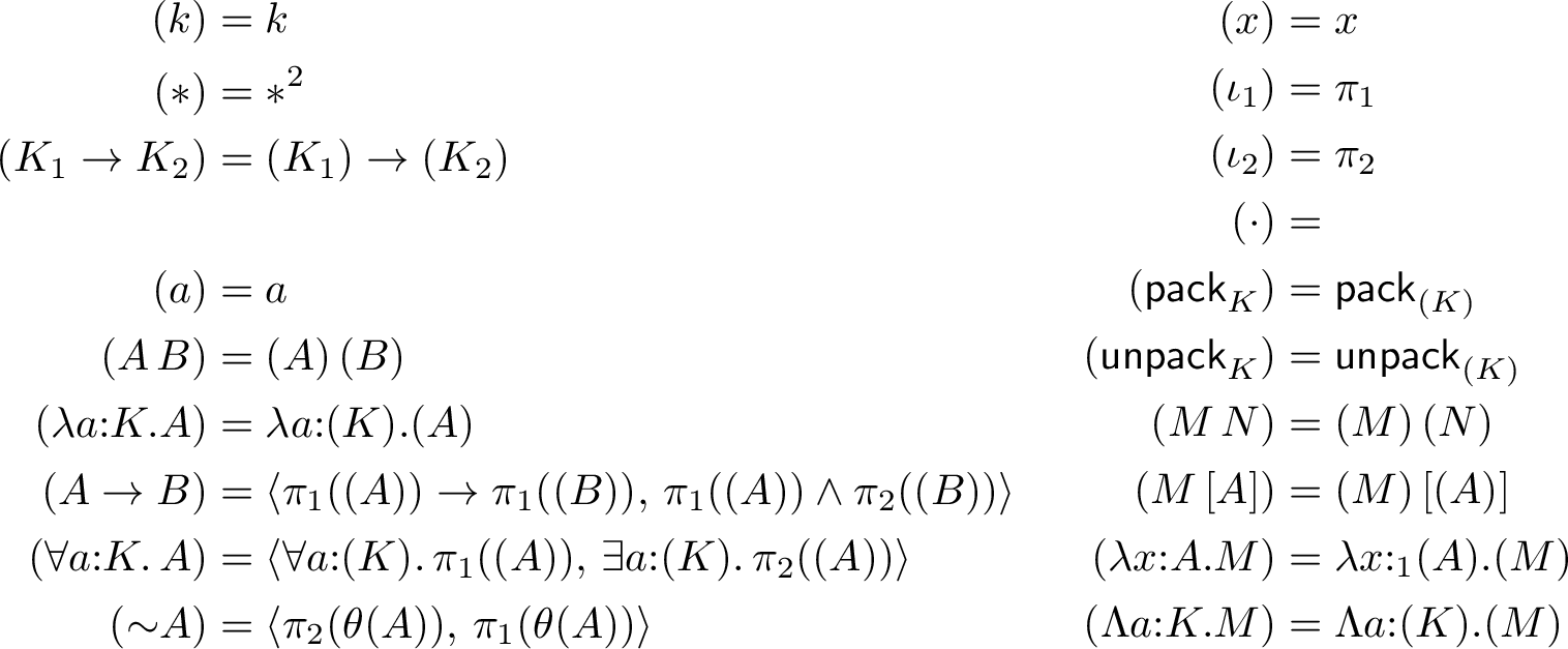
Let us abbreviate \(\pi_i(\theta(A))\) by \(\theta_i(A)\). This way, the fourth clause of the above definition, for example, can be more simply written as \(\theta(A \to B) = \abra{\theta_1(A) \to \theta_1(B),\,\theta_1(A) \wedge \theta_2(B)}\). By an abuse of notation, define the extension of \(\theta_1\) and \(\theta_2\) pointwise over environments by, for each \(i \in \{1,2\}\): \[\begin{align} \theta_i(\emptyset) &= \emptyset\\ \theta_i(\Gamma,a\mathord{:}K) &= \theta_i(\Gamma),a\mathord{:}\delta(K)\\ \theta_i(\Gamma,x\mathord{:}A) &= \theta_i(\Gamma),x\mathord{:}\theta_i(A) \end{align}\]
We show that all three of the mappings interact properly, by demonstrating that proofs of given formulas under assumptions and co-assumptions are preserved.
Lemma 3. Both of the following:
If \(\Gamma \types M : A;\,\Delta\) in then \(\theta_1(\Gamma),\theta_2(\Delta^R) \types \gamma(M) : \theta_1(A)\) in .
If \(\Gamma;\,M : A \types \Delta\) in then \(\theta_1(\Gamma),\theta_2(\Delta^R) \types \gamma(M) : \theta_2(A)\) in .
As a corollary, we obtain the consistency of the system.
Theorem 3 (Consistency). There is no proof term \(M\) such that \(\types M : \PiType{a}{\starsort}{a}\) in .
Proof. Suppose for contradiction that there is such an \(M\). Then by Lemma 3, there is a derivation of \(\types \gamma(M) : \theta_1(\PiType{a}{\starsort}{a})\). By conversion in , there is a derivation of \(\types \gamma(M) : \PiType{a}{\starsort^2}{\pi_1\,a}\). Let \(b\) be a fresh type variable, then by weakening, there is a derivation of \(b\ty:\starsort \types \gamma(M) : \PiType{a}{\starsort^2}{\pi_1\,a}\), and thus one can also derive \(\types \Tyabs{b}{\starsort}{\gamma(M)\,[\abra{b,b}]} : \PiType{b}{\starsort}{b}\). However, this type is not inhabited in . ◻
7 Proofs and Refutations↩︎
In this section, we show a version of the existence property for our system. That is, in any kinding environment, from either a proof of an existential \(\SigmaType{a}{K}{A}\) or a proof of a strongly negated universal \(\sneg{(\PiType{a}{K}{A})}\) one can obtain directly an appropriate witness of kind \(K\).
Unfortunately, our mappings from into of the previous section do not shed much light on this aspect of the system, since the structure of a given proof may be changed quite substantially when undergoing the mapping. For example, a proof \(M\) of a formula \(\SigmaType{a}{(\starsort \to \starsort) \to \starsort}{A}\) is sent to a proof \(\gamma(M)\) of a formula \(\SigmaType{a}{(\starsort^2 \to \starsort^2) \to \starsort^2}{\theta_1(A)}\). So, although the image of the formula is again an existential, it is not clear how one would obtain the correct witness of kind \((\starsort \to \starsort) \to \starsort\) from the witness that has kind \((\starsort^2 \to \starsort^2) \to \starsort^2\), in general.
Therefore, we look to a more fine grained analysis of the structure of proofs and refutations. To this end, define reduction on proof terms as follows.
Definition 16. The relation of proof reduction, written \(M \ped N\), is defined inductively as the contextual closure of the following rules:
Although our mappings from to are not immediately useful to the goal of this section, they do have allow us to obtain one important result very cheaply. Notice that the mapping \(\gamma\) maps redexes to redexes, and is otherwise compatible with the term structure. Consequently, every proof reduction step in can be mirrored, under the mapping, in .
Lemma 4. If \(M \ped N\) in then \(\gamma(M) \pedp \gamma(N)\) in .
Here \(\!\!\mathord{\pedp}\!\!\) is the transitive closure of \(\!\!\mathord{\ped}\!\!\). As a corollary, we obtain strong normalisation.
Theorem 4 (Strong Normalisation). Both of the following:
If \(\Gamma;\,M:A \types \Delta\) then \(M\) is strongly normalising.
If \(\Gamma \types M : A;\,\Delta\) then \(M\) is strongly normalising.
Proof. Suppose \(\Gamma \types M : A;\,\Delta\), the other case is similar. Suppose for contradiction that \(M\) starts some infinite reduction sequence. Then, by Lemma 4, \(\gamma(M)\) also starts some infinite reduction sequence. However, it follows from Lemma 3 that \(\theta_1(\Gamma),\theta_2(\Delta^R) \types \gamma(M) : \theta_1(A)\), contradicting the strong normalisation of . ◻
To futher analyse the structure of proofs, we aim to prove an inversion lemma and a canonical forms lemma. Typically (e.g. in System F\(\omega\)), these lemmas have to take into account that, due to the implicit nature of the rule, a given term may be assigned many different types that are connected by convertibility. In , there is an analogous consideration for the strong negation introduction and elimination rules. Therefore, it is not enough to consider only convertibility, we must take into account that types may be related by pairs of strong negations.
Definition 17. Define binary relation \(A \cong_\beta B\) as the transitive closure of: \[\mathord{\conv} \cup \{(\sneg{(\sneg{A})}, A) \mid A \,\in \mathbb{T}\} \cup \{(A,\sneg{(\sneg{A})}) \mid A\,\in \mathbb{T}\}\] We say that two types \(A\) and \(B\) are neg-convertible* just if \(A \cong_\beta B\).*
Note, however, that this relation is not closed under (one-hole) contexts - the double negation manipulations can only happen at the root of the type. However, it is clear that derivability is closed under neg-convertibility, in the sense that, if \(A \cong_\beta B\) then both: \(\Gamma \types M : A;\,\Delta\) implies \(\Gamma \types M : B;\,\Delta\), and \(\Gamma;\,M:A \types \Delta\) implies \(\Gamma;\,M:B \types \Delta\).
Now we can understand more precisely the necessary conditions under which certain kinds of proof must arise.
Lemma 5 (Inversion). All of the following:
(1) If \(\Gamma \types \tyabs{x}{A}{M} : B;\,\Delta\) and \(B \cong_\beta B_1 \to B_2\) then \(A \conv B_1\) and \(\Gamma,\,x\ty:A \types M : B_2;\,\Delta\).
(2) If \(\Gamma;\,\tyabs{x}{A}{M} : B \types \Delta\) and \(B \cong_\beta\sneg{(B_1 \to B_2)}\) then \(A \conv B_1\) and \(\Gamma,\,x\ty:A \types M : B_2;\,\Delta\).
(3) If \(\Gamma \types \Tyabs{a}{K}{M} : B;\,\Delta\) and \(B \cong_\beta\PiType{a}{K'}{C}\) then \(K = K'\) and \(\Gamma,\,a\ty:K \types M : C;\,\Delta\).
(4) If \(\Gamma;\,\Tyabs{a}{K}{M} : B;\,\Delta\) and \(B \cong_\beta\sneg{(\PiType{a}{K'}{C})}\) then \(K = K'\) and \(\Gamma,\,a\ty:K \types M : C;\,\Delta\).
(5) If \(\Gamma;\,M \cdot_{A_1,A_2} N : B \types \Delta\) and \(B \cong_\beta B_1 \to B_2\) then \(A_1 \conv B_1\), \(A_2 \conv B_2\), \(\Gamma \types M : B_1;\,\Delta\) and \(\Gamma;\,N:B_2 \types \Delta\).
(6) If \(\Gamma \types M \cdot_{A_1,A_2} N : B;\,\Delta\) and \(B \cong_\beta\sneg{(B_1 \to B_2)}\) then \(A_1 \conv B_1\), \(A_2 \conv B_2\), \(\Gamma \types M : B_1;\,\Delta\) and \(\Gamma;\,N:B_2 \types \Delta\).
(7) If \(\Gamma;\,\pack_K\,[\tyabs{a}{K}{A}]\,[C]\,N : B \types \Delta\) and \(B \cong_\beta\PiType{a}{K'}{D}\) then \(K = K'\) and \(A \conv D\) and \(\Gamma \types C : K\) and \(\Gamma;\,N:A[C/a] \types \Delta\).
(8) If \(\Gamma \types \pack_K\,[\tyabs{a}{K}{A}]\,[C]\,N : B;\,\Delta\) and \(B \cong_\beta\sneg{(\PiType{a}{K'}{D})}\) then \(K = K'\) and \(A \conv D\) and \(\Gamma \types C : K\) and \(\Gamma;\,N:A[C/a] \types \Delta\).
Moreover, when a proof (or refutation) is in normal form, then its structure reflects that of the formula that it is proving (or refuting).
Lemma 6 (Canonical Proofs and Refutations). Suppose \(\Gamma\) is a kinding environment and \(N\) is in normal form.
(i) If \(\Gamma \types N : A;\,\Delta\) then:
(a) *If $A$ is neg-convertible with an arrow then $N$ is a term
    abstraction.*

(b) *If $A$ is neg-convertible with a universal type over $K$ then
    $N$ is a type abstraction over $K$.*

(c) *If $A$ is neg-convertible with the strong negation of an arrow,
    then $N$ is a dot construction.*

(d) *If $A$ is neg-convertible with the strong negation of a
    universal type over $K$, then $N$ is a $K$-pack.*
(ii) If \(\Gamma;\,N:A \types \Delta\) then:
 (a) *If $A$ is neg-convertible with an arrow then $N$ is a dot
     construction.*

 (b) *If $A$ is neg-convertible with a universal type over $K$ then
     $N$ is a $K$-pack.*

 (c) *If $A$ is neg-convertible with the strong negation of an
     arrow, then $N$ is a term abstraction.*

 (d) *If $A$ is neg-convertible with the strong negation of a
     universal type over $K$, then $N$ is a type abstraction over
     $K$.*
After first obtaining the preservation of proof reduction under type and term substitutions, a straightforward induction establishes that the type of the subject is preserved under proof reduction.
Theorem 5 (Preservation). Both of the following:
If \(\Gamma;\,M : A \types \Delta\) and \(M \ped N\) then \(\Gamma;\,N:A \types \Delta\)
If \(\Gamma \types M : A;\,\Delta\) and \(M \ped N\) then \(\Gamma \types N:A;\,\Delta\)
By combining the above results, we can finally obtain the existence properties.
Theorem 6 (Existence Property). Suppose \(\Gamma\) is a kinding environment. Then both of:
(i) If \(\Gamma \types M : \SigmaType{a}{K}{A}\) then there is \(B\) and \(N\) such that \(\Gamma \types B : K\) and \(\Gamma \types N : A[B/a]\).
(ii) If \(\Gamma;\, M:\PiType{a}{K}{A} \types\) then there is \(B\) and \(N\) such that \(\Gamma \types B : K\) and \(\Gamma;\,N : A[B/a] \types\).
Proof. Both are similar, so we only do (i). Suppose \(\Gamma \types M : \SigmaType{a}{K}{A} = \sneg{(\PiType{a}{K}{\sneg{A}})}\). Then, by Theorem 4, \(M\) is strongly normalising. Let \(Q\) be a normal form of \(M\). Then, by Theorem 5, \(\Gamma \types Q : \sneg{(\PiType{a}{K}{\sneg{A}})}\). By Lemma 6, \(Q\) is of shape \(\pack_K\,[\tyabs{a}{K}{C}]\,[B]\,N\) and, by Lemma 5, \(C \conv \sneg{A}\) and \(\Gamma \types B : K\) and \(\Gamma;\,N : C[B/a] \types\). Therefore, also \(\Gamma \types N : A[B/a]\) as required. ◻
7.0.0.1 Examples
The ability to construct refutations is very useful under the propositions-as-types paradigm. In what follows we will present some examples that have been inspired by the ideas of Jan De Muijnck-Hughes (and Robert Atkey) for implementing a notion of positive evidence for the falsification of predicates in Idris [17].
Example 4. Suppose we have kinds \(\mathsf{key}\) and \(\mathsf{val}\) and a type \(M : \mathsf{key}\to \mathsf{val}\to \starsort\) describing a particular key-value map. Then we can define the type: \[\abbv{All}_M \mathrel{\vcenter{:}}= \tyabs{p}{\mathsf{val}\to \starsort}{\PiType{x}{\mathsf{key}}{\PiType{y}{\mathsf{val}}{M\,x\,y \to p\,y}}}\] For a given predicate \(P\), a proof \(M : \abbv{All}_M\,P\) is a function that can be used to verify the satisfaction of \(P\) for any key-value pair \((x,y)\) in the map. However, it may be that the codomain of \(M\) does not satisfy \(P\) universally. In this case we may be able to obtain a proof of \(N : \neg\,(\abbv{All}_M\,P)\). However, this seems much less useful: \(N\) is a function which, given an (impossible) proof of \(\abbv{All}_M\,p\), yields a proof of absurdity. Much more useful is to construct a refutation* \(Q : \sneg{(\abbv{All}_M\,P)}\) which consists of witnesses \(K:\mathsf{key}\) and \(V:\mathsf{val}\) together with a proof \(Q_1 : M\,K\,V\) and a refutation \(Q_2 : \sneg{(P\,V)}\).*
Example 5. In higher-order logic it is common to define equality via Leibniz’s principle. This can be formulated as follows in : \[\mathord{=}_K \mathrel{\vcenter{:}}= \tyabs{xy}{K}{\PiType{z}{K \to \starsort}{z\,x \to z\,y}}\] If \(A\) and \(B\) are not equal, then we can attempt to construct a proof \(N : \neg(A =_K B)\), but the computational content of this \(N\) is not so insightful: given an (impossible) proof of the equality of \(A\) and \(B\), we can use \(N\) to obtain a proof of absurdity. On the other hand, a refutation \(Q : \sneg{(A =_K B)}\) amounts to a witness \(P : K \to \starsort\), which is a particular property that is (constructively) satisfied by \(A\) but not \(B\), i.e. there is a proof of \(P\,A\) and a refutation of \(P\,B\).
Example 6. Suppose we have an description of a rooted, directed graph as a kind of nodes \(\mathsf{n}\) and types \(I : \mathsf{n}\), representing the root, and \(E : \mathsf{n}\to \mathsf{n}\to \starsort\), representing the edge relation. Then we can define the type: \[\abbv{Reachable}^{\mathsf{n}}_{I,E} \mathrel{\vcenter{:}}= \tyabs{y}{\mathsf{n}}{\PiType{z}{\mathsf{n}\to \starsort}{z\,I \wedge (\PiType{uv}{\mathsf{n}}{z\,u \wedge E\,u\,v \to z\,v}) \to z\,y}}\] This type encodes a standard second-order definition of reachability, namely that a node \(y\) is reachable from the root whenever every subset of nodes containing the root and closed under the edge relation also contains \(y\). In the case that a given \(Y:\mathsf{n}\) is unreachable, one could attempt a proof \(N : \neg(\abbv{Reachable}^\mathsf{n}_{I,E}\,Y)\), but the computational content of such a proof is not so interesting. By contrast, a refutation* \(Q : \sneg{(\abbv{Reachable}^\mathsf{n}_{I,E}\,Y)}\) consists of a particular edge-closed subset of nodes that contains \(I\) and yet omits \(Y\), in other words, an inductive invariant that certifies the unreachability of (bad state) \(Y\).*
Let us illustrate this example more concretely. Suppose we work in a context containing an axiomatisation of a natural number type. For this simple example, all we will require are:
A kind \(\mathsf{nat}\).
Two type constructors \(0 : \mathsf{nat}\) and \(\mathsf{s}: \mathsf{nat}\to \mathsf{nat}\).
Two proofs witnessing the non-finiteness of \(\mathsf{nat}\): \[\begin{align} h_0 &: \PiType{x}{\mathsf{nat}}{\sneg{(0 = \mathsf{s}\,x)}}\\ h_1 &: \PiType{xy}{\mathsf{nat}}{\sneg{(x = y)} \to \sneg{(\mathsf{s}\,x = \mathsf{s}\,y)}} \end{align}\]
Define a directed graph by \(\abbv{Edge} \mathrel{\vcenter{:}}= \tyabs{xy}{\mathsf{nat}}{y = \mathsf{s}\,x}\) and let us root the graph at \(2\), i.e. define \(\abbv{Init} \mathrel{\vcenter{:}}= \mathsf{s}\,(\mathsf{s}\, 0)\). Then it follows that \(1\) is unreachable, i.e. \(\sneg{({\abbv{Reachable}^\mathsf{nat}_{\abbv{Init},\abbv{Edge}}})}\,(\mathsf{s}\,0)\). Since we are proving the strong negation of a universal, we are forced to supply a witness, which we can take as \(W \mathrel{\vcenter{:}}= \tyabs{n}{\mathsf{nat}}{\SigmaType{m}{\mathsf{nat}}{n = \mathsf{s}\,(\mathsf{s}\,m)}}\). It is easy to prove, by the properties of Leibniz equality, that this set contains \(2\) and is closed under the edge relation. Moreover, we can establish \(\sneg{(W\,(\mathsf{s}\,0))}\), i.e. \(\sneg{(\SigmaType{m}{\mathsf{nat}}{\mathsf{s}\,0 = \mathsf{s}\,(\mathsf{s}\,m)})}\). Since this is equivalent to \(\PiType{m}{\mathsf{nat}}{\sneg{(\mathsf{s}\,0 = \mathsf{s}\,(\mathsf{s}\,m))}}\), it follows directly from \(h_0\) and \(h_1\).
Example 7. In [17], de Muijnck-Hughes defines a new notion of decidability. For a unary predicate \(p\) to be decidable in this alternative sense, there must be a procedure which, for any instance \(x\), either produces a proof of \(p\,x\) or produces a proof of \(q\,x\). In many cases of interest, \(q\,x\) is an Idris type encoding the strong negation of \(p\,x\), but the idea is that one may choose any \(q\) subject to the requirement that \(p\,x\) and \(q\,x\) are inconsistent. In we have strong negation as a primitive, so we may define our own notion9 of strong decidability on kind \(K\): \[\abbv{SDec}_K \mathrel{\vcenter{:}}= \tyabs{p}{K \to \starsort}{\PiType{x}{K}{p\,x \vee \sneg{(p\, x)}}}\] A proof \(M : \abbv{SDec}_K\,P\) for a given predicate type \(P\) is a function which, for any input \(A\) of kind \(K\) produces either a proof of \(P\,A\) or a refutation of \(P\,A\).
8 Conclusion and Related Work↩︎
We have introduced three new two-sided type systems, , and . For the former two, we have shown that derivability of a single-subject judgement in the type system coincides with provability of the corresponding logical sequent of , and its extension with strong negation, respectively. To the best of our knowledge, there is no existing work on extensions of HOL with strong negation, but we have shown that our system is consistent, strongly normalising and satisfies the existence and dual existence properties. Since each of these systems can be naturally understood as an extension of the core rules of two-sided type systems, as identified in [1], [2], this gives a reasonable explanation of the logical foundations of two-sided type systems through the lens of propositions-as-types.
8.0.0.1 Two-sided type systems
Our systems extend the pure \(\lambda\)-calculus rules identified in the introduction to [1] and which were refined and augmented with complementation in [2]. Those works did not consider logical aspects except to illustrate the connection between their co-arrow and logical co-implication. In our work, the intended meaning of a typing formula \(M:A\) on the left-hand side of the judgement, namely that \(M\) is a refutation of \(A\), is rather stronger. This is necessary for the soundness of our rules. In the previous works, the intended meaning of such a typing formula is \(M\) is not a term of type \(A\). For example, the following is an instance of our of :
_1(M) : A
If we know only that \(M\) is not a term of type \(A \vee B\), it is not sound to conclude that \(\pi_1(M)\) is not a term of type \(A\). The former can be satisfied by \(M \mathrel{\vcenter{:}}= (P,Q)\) for some \(P:A\). However, if we know that \(M\) is a refutation of \(A \vee B\), then, indeed, \(\pi_1(M)\) must be a refutation of \(A\).
8.0.0.2 Bilateral Logics
Bilateralism can be understood as a part of proof theoretic semantics in which dual concepts in logic, such as assertion and denial, or proof and refutation, are considered symmetrically, and given equal importance [18]. It is natural, therefore, that we should take a bilateral logic as the basis for the correspondence with two-sided typing. Our system is in correspondence with Wansing’s , which is a bilateral natural deduction system that was introduced in [3]. Wansing illustrated how bilateral systems such as can be naturally extended with the strong negation operation in [19], although he did not define a specific, named system. It was recently shown, in a manuscript published on the Arxiv, that strong negation is actually definable in using the coimplication [16]. We have not gone down that route, and instead defined explcitly, because our goal is to understand the correspondence with the two-sided rules of Figure 1.
The coimplication is a key feature of Wansing’s logic. A related line of work studies (non-bilateral) accounts of intuitionistic logic extended with coimplication, starting with Rauzer’s Heyting-Brouwer logic [20], and more recently the works of Crolard [21], [22], [23], [24] and [7]. However, excepting the latter, the lack of a symmetrical treatment of refutation causes these logics to loose some of the good properties of intuitionistic logic, such as the disjunction property. The work of [7] retains the disjunction property, although the authors do not define a proof system.
Ayhan constructed a \(\lambda\)-calculus \(\lambda^{\mathsf{2Int}}\) in correspondence with in [25]. This calculus is obtained by annotating with 2-sorted \(\lambda\)-terms, so it is not given in a sequent format and there are two distinct judgements corresponding to proof and refutation. Like our two-sided type system (and ), there is a notion that terms are assigned types under a pair of assumptions and co-assumptions, but unlike , proof terms and refutation terms are distinct: every term construction, except for truth and falsity, has separate positive and negative forms. Consequently, in \(\lambda^{\mathsf{2Int}}\) and unlike the systems of this paper, terms have unique principal types. Otherwise, the relationship between Ayhan’s system and our system seems reasonably clear. [26] constructed a \(\lambda\)-calculus corresponding to Rumfitt’s bilateral natural deduction [10], but it is a symmetric calculus in the style of [27].
8.0.0.3 Strong Negation
We identified the concept of strong negation as the logical counterpart to the complementation rules of Figure 1. Strong negation was introduced by Nelson in [4] as a replacement for intuitionistic negation. In particular, the work was motivated essentially by the property that is nowadays often called constructible falsity. This is the first formalization of Nelson-style constructible falsity, which is later known as N3. Nelson also presented a Hilbert-style calculus for this logic, but its metatheory remained tied to the arithmetical framework in which he was working. Later work separated Nelson-style strong negation from this arithmetical background. One of the earliest natural-deduction presentations of Nelson-style strong negation appears in Prawitz’s 1965 work [28]. Gurevich later treated the system as a pure logic: he developed a Hilbert calculus, established a Kripke semantics and completeness theorem, and presented a corresponding Gentzen-style calculus [15]. Almukdad and Nelson introduced the paraconsistent Nelson logic N4, which weakens N3 by allowing inconsistency without triviality [29].
In his monograph [11], Wansing constructed a \(\lambda\)-calculus corresponding to a version of N4, called \(\lambda^c\). As our systems, the strong negation has no associated introduction or elimination form at the term level. Consequently, proofs and refutations are identified so that, for example, every term of type \(\sneg{(A \wedge B)}\) is also of type \(\sneg{A} \vee \sneg{B}\). Wansing’s \(\lambda^c\) is presented in Church style, with terms annotated by their types, and his correspondence is with a Gentzen-style system. The system is not bilateral and only treats the propositional case.
De Muijnck-Hughes, partly inspired by Atkey’s incorporation of a version of strong negation in inductive datatypes [30], has implemented a notion of positive evidence for the falsification of predicates in Idris [17]. In a talk at TRIPLES in Edinburgh, he set out very clearly the benefits of the approach compared to proving an intuitionistic negation, and this has been the inspiration for our examples of Section 7. Atkey’s work also contains a semantics for datatypes with negation based on Chu-spaces, which is closely related to our mapping \(\theta\), since it models types as pairs of their positive and negative evidence, and interprets negation as transposition.
8.0.0.4 Higher-Order Logic
Our system is a two-sided version of Geuvers’ [5], [13], which itself corresponds to the higher-order logic in Church’s Simple Theory of Types [6]. Our system is both bilateral and incorporates a strong negation, but we are not aware of any existing work on either higher-order logics or type systems that combine both of these features.
References↩︎
Actually, only and are given explicitly in [2]. However, rules and are admissible via the subtyping equivalence \((A^c)^c \equiv A\). We add them here explicitly since we will not consider subtyping in this work.↩︎
It is unfortunate that \(A \coto B\), which is semi-standard notation for coimplication, clashes with the so-called ‘necessity’ arrow of [1], [2]. However, since we will not consider that type any further it should not lead to a misunderstanding.↩︎
This property is known under the name Construbtible Falsity in some literature (e.g. [7]). Here, we choose the name Constructible Refutation, in order to distinguish the property from Nelson’s notion of constructible falsity in [4] and the subsequent Nelson family logics.↩︎
This notion, which we will refer to as Nelson-style constructible falsity, is also more commonly called strong negation directly nowadays. Although it is motivated by a requirement analogous to Constructible Refutation, that property alone does not uniquely determine Nelson’s connective; other notions of negation may also satisfies Constructible Refutation.↩︎
Here bilateral can be understood as: giving equal import to proof and refutation. The term originates with Rumfitt [10].↩︎
[3] denoted this as \(A \wcoto B\), that is, a 180 left-right flip of \(A \coto B\). We use the latter instead, to align better with [2].↩︎
The strong negation is definable in [16], and is conservative over intuitionistic propositional logic [3], but this formula is not intuitionistically valid.↩︎
However, the fact that conjunction is a defined operator complicates this particular example.↩︎
Note, our notion and de Muijnck-Hughes’ are generally incomparable since we do not assume that \(A\) and \(\sneg{A}\) are inconsistent.↩︎