Transition-Aware Routing in Hybrid Hollow-Core/Single-Mode Fiber Networks: A Cost–Throughput Investigation
July 15, 2026
1 Introduction↩︎
The gradual transition from all-SMF optical networks to hybrid HCF/SMF infrastructures introduces a routing cost that conventional optical-network models do not capture. That cost is not the ordinary in-span fusion splice—low-loss and already in every network’s per-kilometer loss budget—but the fiber-type transition itself. Each HCF\(\leftrightarrow\)SMF interface is a mode-field-mismatch junction needing a specialized coupler with higher, more variable loss, and is simultaneously a discontinuity in chromatic dispersion (CD), group velocity, span-loss profile, and nonlinearity that forces the downstream erbium-doped fiber amplifier (EDFA) to retarget its gain [1]. These costs arise only where fiber type changes, so they are absent in all-SMF or all-HCF backbones and grow with the number of transitions a route crosses. A route attractive under length or GSNR alone may thus be undesirable once transitions are counted, while avoiding them too aggressively forces detours that lengthen paths, cut GSNR margin, and hurt carried traffic. The design question is therefore not whether transition awareness helps, but when the reduction in cross-fiber transitions is worth the routing cost it introduces.
This question sits at the intersection of two established lines of work. The first is impairment-aware routing and spectrum assignment (RSA), where shortest-path, disjoint-path, and quality-of-transmission (QoT)-aware provisioning methods are commonly built on Yen-style K-shortest paths, Suurballe-type protection, and Gaussian-noise (GN) model-driven GSNR estimation [2]–[10]. These methods are mature and effective, but they usually use physical length or inverse GSNR as the routing weight, which leaves fiber type invisible during path selection. The second line is the emerging literature on HCF systems and networks. HCF has matured toward transport-grade deployment: recent antiresonant designs reach attenuation at or below the silica Rayleigh floor—0.091 dB/km, and below 0.2 dB/km across a 66 THz window [11]—while preserving HCF’s low latency and extremely weak Kerr nonlinearity [11]–[16]. At the same time, the relevant penalties are now better understood, including intermodal interference (IMI), HCF-to-SMF splice loss, and \(CO_2\) absorption in L-band operation [17]–[27].
What remains less developed is the routing-decision layer for dynamic protected provisioning in hybrid topologies. Prior work has examined HCF placement, hybrid HCF/SMF planning, and joint fiber, modulation, and spectrum allocation, and a companion study has considered protection switching on the same topology family [1], [28]–[30]. Dynamic impairment-aware provisioning itself is mature—ABACUS jointly optimizes routing, modulation, and spectrum under a QoT constraint [31], and Ouyang et al. allocate routing, fiber, modulation, and spectrum for hybrid ultra-low-loss/standard-SMF links [30]. But their objectives are either fiber-type-blind or fix fiber type at planning time (which link gets which fiber) rather than pricing a per-route transition cost during path selection. To our knowledge, no prior work prices HCF\(\leftrightarrow\)SMF transitions explicitly in the routing objective for dynamic, dedicated-protection provisioning, and the practically important middle ground between ignoring transitions and minimizing them aggressively is likewise unexplored, especially where the operator wants some transition awareness but not arbitrary detours.
This paper addresses that gap with a controlled comparison of six protected routing schemes on a common event-driven simulator, spanning fiber-blind and GSNR-aware baselines through to explicitly transition-aware designs. To make transitions visible without abandoning the GN-model framework, a per-transition GSNR penalty—calibrated from HCF–SMF splice loss and the EDFA gain transients induced at reconfigurable optical add/drop multiplexers (ROADMs)—is applied at the feasibility stage, symmetrically across all schemes, so even a fiber-blind objective pays the physical-layer cost of transitions at provisioning time. A composite per-demand availability metric with an exploratory splice-related failure term, computed with the ITU-T G.911 steady-state methodology (its failure rates from field cable-cut statistics and a conservative splice assumption), serves as a reliability cross-check rather than an optimization target. Two middle-ground constructions are introduced to fill the gap between familiar baselines and aggressive transition minimization: GMR-T keeps the candidate set of GSNR-maximal routing (GMR) but reranks feasible candidates by transition count, while BD-TPAR scheme retains the transition awareness of the TPAR scheme but caps the detour length and falls back to GMR when no capped candidate exists. The paper thus (i) compares six schemes under a common transition-penalized feasibility model, (ii) introduces two intermediate designs that make transition awareness practical, and (iii) converts the trade-off into a decision rule mapping operator cost structure to scheme choice. The results show that the preferred scheme depends on deployment pattern and cost regime rather than on a universal ranking: BD-TPAR emerges as the practical default under fragmented rollout, GMR-T as a lower-complexity alternative, DA-RSA or GMR as sufficient when no explicit transition cost is carried, and TPAR or the GFJ scheme as justified only when transition cost is high enough to warrant the extra detour.
Section 2 describes the model; Section 3 the six schemes; Section 4 the parameters; Section 5 the results; and Section 6 the decision rule.
2 System Model↩︎
![Figure 1: Overview. (a) A 1+1-protected demand traverses HCF and SMF segments; each HCF\leftrightarrowSMF transition (\eta) adds splice loss and an EDFA gain transient to the Extended-GSNR feasibility budget [2 ] and an exploratory splice-failure term to the availability model (Section 2.5). (b) CORONET fiber-type map at 50% HCF under uniform-random deployment (one seed); the interleaving of HCF (blue solid) and SMF (red dashed) drives the high per-route transition counts. (c) The six schemes organized by how strongly path selection weights transitions: fiber-blind baselines (DA-RSA, GMR), the middle-ground schemes introduced here (GMR-T, BD-TPAR), and the explicit minimizers (TPAR, GFJ).](/article/2607.14324/_pdflatex/qmezsdup.png "fig:")
2.1 Topology ensemble and fiber assignment↩︎
We use six published reference topologies: CORONET (30), COST239 (11), NSFNET (14), USNET (24), and COST266 (37) and Nobel-Germany (17). The HCF deployment fraction is swept over \(p_\text{HCF}\in\{0,0.25,0.5,0.75,1.0\}\); the default assignment marks a uniformly random edge subset as HCF until the count reaches \(p_\text{HCF}\,|E|\) (requiring no operator coordination), and as an alternative we also consider a contiguous breadth-first-search (BFS)-expanded HCF cluster grown from a random seed link (Section 5.4). For each \((\text{topology},p_\text{HCF},\text{seed})\) triplet, all six schemes see the same deterministic HCF link set and the same random variates—identical source–destination pairs and holding-time draws from a fixed seed—so scheme comparison is paired by construction. Across loads the arrival rate is scaled by the Erlang value while these variates are held fixed, so the load sweeps vary offered load without changing the underlying demand realization.
2.1.0.1 How the hybrid plant is implemented.
Fiber type is assigned at link granularity: a link is all-HCF or all-SMF over its whole length and is operated as a chain of single-type amplified spans (80 km for SMF, 100 km for antiresonant HCF (AR-HCF); Table 1), with amplified spontaneous emission (ASE) noise and nonlinear interference (NLI) accumulated under per-fiber locally-optimized (LOGO) launch power, capped so the full-fill aggregate stays within a 23 dBm booster ceiling. Since LOGO makes the per-span GSNR invariant along a uniform-fiber link, we accumulate inverse-GSNR by scaling one reference span’s value by the link length rather than summing spans individually. No link mixes fiber types, so HCF\(\leftrightarrow\)SMF interfaces occur only at ROADM nodes where a route changes fiber type; \(N_\text{trans}(P)\) counts these handovers, and each link’s latency follows its own group index.
2.2 Extended GN model with IMI↩︎
The per-link GSNR is the incoherent GN-model accumulation [8] \[\frac{1}{\mathrm{GSNR}_\mathrm{ext}}=\frac{1}{\mathrm{GSNR}_\mathrm{ASE}} +\frac{1}{\mathrm{GSNR}_\mathrm{NLI}}+\frac{1}{\mathrm{GSNR}_\mathrm{IMI}}, \label{eq:extgn}\tag{1}\] with standard ASE and NLI terms; the IMI term is non-zero only on HCF links and scales linearly with length. CO2 absorption on L-band HCF enters through the wavelength-dependent loss \(\alpha(\lambda)\) (Section 1), hence through the ASE term. The NLI term grows with the number of lit channels. To keep routing fast we do not recompute the GSNR on every arrival: each link’s occupancy is classified as low, med, or high (breakpoints near one third and two thirds of the 80 channels, with a small hysteresis band), the GSNR is precomputed once per state, and a link’s routing weight changes only when its occupancy class changes. Figure 1 sketches the hybrid-path structure and the design space of the six schemes, and Table 1 lists the fixed fiber parameters.
| Parameter (C / L) | SMF (G.652) | AR-HCF |
|---|---|---|
| \(\alpha\) [dB/km] | 0.20 / 0.21 | 0.13 / 0.14 |
| \(D\) [ps/(nm\(\cdot\)km)] | 17.0 / 20.0 | 3.5 / 4.0 |
| \(\gamma\) [W\(^{-1}\)km\(^{-1}\)] | 1.3 / 1.15 | \(10^{-3}\) |
| \(n_g\) | 1.468 | 1.0003 |
| Span length [km] | 80 | 100 |
| EDFA NF (C / L) [dB] | 5.5 / 6.5 | 5.5 / 6.5 |
| IMI MPI level [dB/km] | — | \(-55\) / \(-53\) |
| Pulse roll-off \(\alpha_\text{RRC}\) | 0.10 | 0.10 |
2.3 Per-transition GSNR penalty↩︎
Each HCF\(\leftrightarrow\)SMF interface costs the physical layer an SNR budget independent of the routing weight, which we model as a per-transition penalty \(\eta_\text{trans}\) calibrated from two literature-informed contributions. First, HCF–SMF splice/coupler loss, which recent work has reduced from about 1.2 db (early angle-cleaved splices) to 0.15 db on antiresonant nodeless designs [23]; we adopt 0.3 db as a conservative mid-range value. Second, the ROADM-induced EDFA gain transient: cascaded EDFAs in colorless–directionless–contentionless (CDC) ROADMs react to add/drop events with surviving-channel excursions of several decibels that gain-control loops must suppress srivastava1997edfatancevski1999swings?, and residual gain-ripple and filter-shape uncertainty is a recognized QoT-margin component [32]; we attribute a conservative 0.1 db per transition to gain re-targeting at each fiber-type boundary. This second term is an order-of-magnitude modeling estimate, not a measured value: the cited work establishes that such transients exist and consume margin, but to our knowledge no study reports a single calibrated per-transition GSNR figure. We therefore treat \(\eta_\text{trans}=\SI{0.4}{\decibel}\) as a nominal operating point whose influence on the ranking is bounded by the sweep of Section 5.5. It is applied symmetrically (splice loss is reciprocal) and subtracted from the path-level Extended-GSNR (in dB), \[\mathrm{GSNR}_\mathrm{ext}^\text{path}= -10\log_{10}\!\Big(\textstyle\sum_{i\in P}1/\mathrm{GSNR}_\mathrm{ext}^{(i)}\Big) -N_\text{trans}(P)\,\eta_\text{trans}, \label{eq:eta95trans}\tag{2}\] where \(N_\text{trans}(P)\) counts transitions on path \(P\). The penalty is charged at the feasibility test on both paths of a 1+1 demand (each must clear its threshold post-switchover), but the transition-aware objectives and the reported per-demand count \(\bar{n}\) (Fig. 3 (b)) score the working path only—the path carrying traffic in normal operation. Being a feasibility test rather than a routing objective, the penalty is paid by every scheme regardless of whether its path-selection objective weights \(N_\text{trans}\). Digital-signal-processing (DSP) equalizer reconvergence is deliberately excluded: modern 1+1 deployments run both paths in hot standby with pre-converged DSP, so switchover is electrical selection [33] and that cost surfaces as transponder resource use rather than per-channel GSNR. Throughout, \(\eta_\text{trans}=\SI{0.4}{\decibel}\) should be read as a calibrated sensitivity parameter that sets the operating point of the study, not as a measured universal constant; Section 5.5 sweeps it over \([0,1]\) dB and shows that the scheme ranking is insensitive to the calibration.
2.4 Provisioning constraints and dynamic traffic↩︎
Four dual-polarization (DP) formats {DP-QPSK, DP-8QAM, DP-16QAM, DP-64QAM} carry GSNR thresholds \(\theta_\text{mod}\in\{10,13,16,22\}\) dB; provisioning requires \(\mathrm{GSNR}_\mathrm{ext}^\text{path}\ge\theta_\text{mod}+m\) with a 1 db margin \(m\), where \(\mathrm{GSNR}_\mathrm{ext}^\text{path}\) is the end-to-end (path-level) GSNR of 2 —the incoherent sum of per-link inverse-GSNR less the transition penalty—not a per-link threshold. The selector picks the highest-spectral-efficiency format that passes. For a 1+1 demand the binding constraint is the worse of the working and protection path-level GSNRs. The study band comprises 80 channels on a 75 GHz grid (64 GBd) spanning 191.307–197.232 THz (1520.0–1567.1 nm), a 6 THz window that extends past the conventional C-band (1530–1565 nm) on the short-wavelength side, in the spirit of extended/super-C-band systems; we retain the label “C-band” for brevity. The grid is wavelength-continuity-constrained with no converters; first-fit assignment ORs (bitwise logical) the per-link occupancy bitmaps of the working/protection pair and takes the lowest free index. C-band CO2 absorption is an order of magnitude weaker than in the L-band [34] and is not modeled. The permitted working-versus-protection latency asymmetry is bounded per topology by \[\Delta\tau_\mathrm{max}=\beta\,\bar{L}_\mathrm{sp}\, \left|\frac{1}{v_{g,\mathrm{SMF}}}-\frac{1}{v_{g,\mathrm{HCF}}}\right|, \label{eq:dtmax}\tag{3}\] with \(\bar{L}_\mathrm{sp}\) the mean shortest-path length, \(\beta=0.60\), and \(v_{g,f}=c/n_g^{(f)}\); the bound is enforced as a hard constraint (HC1). It exists because the receiver must realign the two continuously arriving 1+1 copies within a finite differential-delay buffer for switchover to be hitless. In all-SMF networks the asymmetry comes from length differences alone and is rarely binding; in a hybrid plant the \(\sim\)1.6 μs/km group-delay gap between HCF and SMF [1] makes it first-order. 3 scales the allowance to the topology: the group-delay term is the asymmetry a mean-length route would accumulate if one path were all-SMF and the other all-HCF, and \(\beta=0.60\) grants 60% of that worst case as buffer budget. Each trial issues \(N=3{,}000\) requests (600 warm-up, 2400 measurement) with Poisson arrivals at rate \(\rho/H\) (\(\rho\) in Erlangs, mean holding \(H=\SI{1}{hour}\)) and uniform source–destination pairs; every operating point runs ten seeds, and all figures report 95% confidence intervals over the seeds.
2.5 Composite per-demand availability↩︎
Each accepted 1+1 demand is scored with the standard repairable series/parallel model [35]: the working path is a chain of \(N_\text{L}^{(w)}\) cable spans and \(N_\text{trans}^{(w)}\) splice joints (likewise the protection path), and the demand is up if and only if either path is up. With per-link cable and per-splice availabilities, each set by a failure rate \(\lambda\) and a mean time to repair (MTTR), \[a_\text{cab}=\frac{1}{1+\lambda_\text{cab}\,\mathrm{MTTR}_\text{cab}},\qquad a_\text{spl}=\frac{1}{1+\lambda_\text{spl}\,\mathrm{MTTR}_\text{spl}},\] we adopt \(\mathrm{MTTR}_\text{cab}=\SI{12}{\hour}\)—the Bellcore cable-cut repair time tabulated by To and Neusy [36]—and a deliberately conservative cable-cut rate \(\lambda_\text{cab}=\SI{1e-4}{\per\hour}\), of the same order as the reported field statistic of 4.39 cable cuts per 1000 sheath-miles per year [36] (\(\sim\SI{3e-5}{\per\hour}\) per 80–100 km span); the steady-state form itself follows the ITU-T G.911 methodology [37]. The splice term deserves a caveat: production fusion splices are normally treated as passive and effectively failure-free in availability planning, and no per-splice outage rate is standardized. We include splice reliability as a conservative what-if, since ITU-T G.911 lists splices and connectors as fiber-plant reliability parameters [37]. We assume \(\lambda_\text{spl}=\SI{1e-5}{\per\hour}\) and \(\mathrm{MTTR}_\text{spl}=\SI{6}{\hour}\), with a failure rate ten times lower than that of the cable. The purpose is to test whether transition-aware routing could ever earn a reliability benefit; Section 5.8 shows the answer is negative at any plausible rate, so this choice drives no conclusion. Per-path availability is the series product \(A^{(w)}=a_\text{cab}^{\,N_\text{L}^{(w)}}\,a_\text{spl}^{\,N_\text{trans}^{(w)}}\), and the 1+1 composite adds a coarse channel-outage term keyed to a single binary label (whether the working path is majority-HCF)—a first-order model, not a per-link fiber-aware reliability calculation, meant only to bound whether transition count could reorder the schemes on availability. Only the splice term depends on \(N_\text{trans}\); its impact is swept in Section 5.8.
3 Routing Schemes↩︎
All six schemes run on a common provisioning loop (Section 3.7) and all six pay the per-transition GSNR penalty of 2 at the feasibility check; they differ only in how strongly path selection weights transitions, from not at all (DA-RSA, GMR), through the soft middle-ground designs introduced here (GMR-T, BD-TPAR), to explicit minimization on a state-augmented graph (TPAR, GFJ), as organized in Fig. 1 (c).
3.1 DA-RSA: distance-adaptive RSA↩︎
The DA-RSA baseline performs Yen’s K-shortest-paths (K-SP) search [2] on physical link length and uses the Extended-GSNR feasibility check (2 , including the per-transition penalty) to discard infeasible candidates. The highest-spectral-efficiency modulation format passing the threshold-plus-margin inequality is selected, and among feasible candidates the shortest-length path is chosen. We use \(K=5\) candidate paths per demand, for all schemes. QoT-aware RSA studies typically use \(K\in[3,10]\) [4], [8]: below \(\sim\)3 sparse topologies often lack a feasible working/protection pair; beyond \(\sim\)5 the extra candidates are longer variants that rarely pass the GSNR gate while runtime grows linearly in \(K\). \(K=5\) is the midpoint, held fixed across schemes for fairness. DA-RSA does not weight HCF\(\leftrightarrow\)SMF transitions in its objective, but transitions still drive its blocking probability by reducing the post-penalty GSNR of transition-heavy candidates below the modulation threshold.
3.2 GMR: GSNR-maximal routing↩︎
GMR uses the per-link inverse Extended-GSNR as a Dijkstra edge weight, \(w_{ij}^\text{GMR} = 1/\mathrm{GSNR}_\text{ext}^{(ij)}\). Summing along a path recovers the inverse end-to-end GSNR before the transition penalty, so the shortest-weight path is the highest-pre-penalty-GSNR path. The post-routing feasibility check applies 2 – meaning that, like DA-RSA, GMR sees transitions only at the feasibility gate. GSNR-shortest paths nevertheless tend to favor HCF (higher per-link GSNR), which is transition-light, giving GMR an implicit advantage on hybrid topologies (Section 5).
3.3 GMR-T: GMR with K-best transition reranking↩︎
GMR-T uses the same candidate generator as GMR – Yen’s K-shortest-paths on the per-link inverse-Extended-GSNR – but deviates from GMR in the selection step. Instead of taking the GMR-first feasible candidate, GMR-T enumerates the entire \(K\)-best set, applies the same feasibility checks (HC1–HC3), and selects the feasible candidate with the lowest cross-fiber transition count, breaking ties by GMR cost. Concretely, among the feasible set \(\mathcal{F}\subseteq\{1,\ldots,K\}\), GMR-T picks \[k^\star = \arg\min_{k\in\mathcal{F}} \bigl(N_\text{trans}(P_k), -\mathrm{GSNR}_\text{ext}^{(P_k)}\bigr), \label{eq:gmrt95select}\tag{4}\] under lexicographic ordering. GMR-T inherits GMR’s \(O(K|E|\log|V|)\) per-event Yen runtime and adds only an \(O(K)\) post-feasibility comparison. When no transition-cheaper alternative exists in \(\mathcal{F}\), GMR-T degenerates exactly to GMR; when one does, GMR-T captures the reduction without an explicit detour penalty—its candidates are confined to GMR’s \(K\)-best set, though the selected lower-transition candidate may be marginally longer than the GMR-optimal one.
3.4 BD-TPAR: bounded-detour TPAR↩︎
BD-TPAR runs the TPAR augmented-graph candidate generator (Section 3.5) but enforces a hard cap on the working path’s physical length. Let \(L^\star(s,d)\) denote the length of the shortest physical \(s\!\to\!d\) path (a single Dijkstra computation on physical lengths). For each augmented candidate \(P_k\), BD-TPAR accepts \(P_k\) only if \[L(P_k) \le \delta\,L^\star(s,d), \label{eq:bd95tpar95cap}\tag{5}\] with \(\delta\ge 1.0\) a tunable parameter (we use \(\delta=1.2\) as default, i.e., a working path may detour at most 20% past the shortest physical path to avoid a transition). If no TPAR-augmented candidate fits the cap, BD-TPAR falls back to the GMR candidate set, so its coverage is never strictly worse than GMR’s. At \(\delta=1.0\) BD-TPAR collapses to a GMR-like scheme; at \(\delta=\infty\) it collapses to TPAR; in between, \(\delta\) is an explicit, operator-tunable detour budget.
3.5 TPAR: transition-penalty-aware routing↩︎
TPAR makes the per-transition penalty part of the path-selection objective itself. We build a state-augmented graph on the Cartesian product of the physical node set and the fiber-type set \(\{\text{HCF}, \text{SMF}\}\): each physical node \(v\) becomes a pair of augmented nodes \((v, \text{HCF})\) and \((v, \text{SMF})\) distinguished by the incoming fiber type on the edge that reached them. An augmented edge from \((u, f_\text{in})\) to \((v, f_\text{out})\) exists if and only if a physical link \(u\to v\) of fiber type \(f_\text{out}\) exists, with cost \[w^\text{TPAR}_{(u,f_\text{in})\to(v,f_\text{out})} \;=\; \frac{L_{uv}}{L_\text{max}} \;+\; P[f_\text{in}, f_\text{out}], \label{eq:tpar95weight}\tag{6}\] where \(L_{uv}\) is the link length normalized by the topology diameter and \(P\) is a \(2\!\times\!2\) transition-penalty matrix whose diagonal is zero and whose off-diagonal entries encode the relative cost of HCF\(\to\)SMF vs.SMF\(\to\)HCF crossings (Section 4). A K-shortest-paths search on the augmented graph—implemented by iterative single-edge exclusion rather than strict Yen spur-path bookkeeping, which yields the same \(K\) physically-distinct paths in ascending cost—returns candidate paths whose total cost contains both a length term and an explicit transition count. This state augmentation extends the K-shortest-paths framework [2] with the type-of-incoming-fiber state.
3.6 GFJ: joint GSNR-plus-transition routing↩︎
GFJ replaces TPAR’s additive length+penalty form with an additive (unnormalized) combination of inverse-GSNR cost and transition cost on the same augmented graph: \[w^\text{GFJ}_{(u,f_\text{in})\to(v,f_\text{out})} \;=\; \frac{1}{\mathrm{GSNR}_\text{ext}^{(uv)}} + \lambda_\text{GFJ}\, P[f_\text{in}, f_\text{out}], \label{eq:gfj95weight}\tag{7}\] with a single tunable scalar \(\lambda_\text{GFJ}\in[0,1]\). At \(\lambda_\text{GFJ}=0\) GFJ reduces to GMR on the augmented graph; increasing \(\lambda_\text{GFJ}\) adds a transition-penalty term of growing weight on top of the (always-retained) inverse-GSNR cost. Because the inverse-GSNR term (\(\mathcal{O}(10^{-2})\) per edge) and the penalty term (\(\mathcal{O}(1)\) per transition) are on very different numerical scales, even a small \(\lambda_\text{GFJ}\) makes the penalty dominate; the practical consequence of this is the sharp-threshold behavior: even small \(\lambda_\text{GFJ}\) values drive blocking and carried-traffic performance to saturate near the TPAR level, leaving little usable middle ground. We use \(\lambda_\text{GFJ}=0.3\) throughout, placing the scheme firmly in the saturated regime.1
3.7 Unified provisioning loop↩︎
For each incoming demand the provisioning loop produces up to \(K=5\) candidate working-paths from the scheme-specific router along with a link-disjoint protection path. The procedure for each candidate is: (i) enforce the latency-asymmetry hard constraint \(|\tau_\text{work}-\tau_\text{prot}| \le \Delta\tau_\mathrm{max}\) (HC1); (ii) apply the Extended-GSNR feasibility check of 2 with a 1 dB margin on both the working and the protection path (HC2); (iii) find the lowest-index wavelength that is free on every link of both paths, using a vectorized bitmap OR (HC3); (iv) commit the wavelength and release it on the demand’s departure event. Blocking is recorded by the first gate each rejected demand fails. In the current router a demand can fail at one of four points – latency-asymmetry (HC1), GSNR-infeasibility (HC2), no common wavelength (HC3), or no link-disjoint working+protection pair (“no-working-path”) – and these four rates sum exactly to the overall blocking probability.
4 Parameter Settings↩︎
Section 5 uses one fixed setting per free parameter, listed in Table 2. The transition-penalty matrix encodes the asymmetric per-direction operational cost of fiber-type crossings: HCF\(\to\)SMF crossings cost more than SMF\(\to\)HCF crossings because the EDFA on the SMF side following the splice must lift its gain to cover both the splice loss and the higher SMF span loss, producing a larger gain-transient excursion. The per-transition penalty \(\eta_\text{trans}\) is swept in Section 5.5; all other parameters are held fixed.
| Parameter | Value |
|---|---|
| Candidate-path count \(K\) (Yen’s K-SP) | 5 |
| GFJ transition weight \(\lambda_\text{GFJ}\) | 0.3 |
| BD-TPAR detour cap \(\delta\) | 1.2 |
| Per-transition GSNR penalty \(\eta_\text{trans}\) | 0.4 db |
| Engineering margin \(m\) | 1.0 db |
| Transition matrix (H\(\to\)S, S\(\to\)H) | 1.00, 0.89 |
| Quasi-dynamic weight-table dead-band | 4–6 channels |
| Latency-asymmetry limit \(\Delta\tau_\text{max}\) | [eq:dtmax] |
| Cable failure rate \(\lambda_\text{cab}\) | 1 × 10⁻⁴ h |
| Splice failure rate \(\lambda_\text{spl}\) | 1 × 10⁻⁵ h |
| Cable MTTR \(\mathrm{MTTR}_\text{cab}\) | 12 h |
| Splice MTTR \(\mathrm{MTTR}_\text{spl}\) | 6 h |
5 Results — C Band↩︎
All numerical results in this section are drawn from 10 800 trials (6 topologies \(\times\) 5 HCF fractions \(\times\) 6 loads \(\times\) 10 seeds \(\times\) 6 schemes) with 3 000 events per trial (600 warm-up, 2 400 measurement), plus two dedicated sensitivity sweeps (the \(\eta_\text{trans}\) sweep and the contiguous-rollout comparison) run at the same headline operating point of 50% HCF and 300 Erlang. The per-transition GSNR penalty \(\eta_\text{trans}=\SI{0.4}{\decibel}\) and the BD-TPAR detour cap \(\delta=1.2\) are active throughout. Unless noted, a scheme’s carried-traffic lift is the mean over the six topologies of its per-topology percentage lift relative to DA-RSA; pooling demands across topologies instead shifts the figures by 1–2 points but not the ranking. The section runs from headline results to mechanism, ending with the L-band and availability cross-checks.
5.1 Blocking probability vs.load↩︎
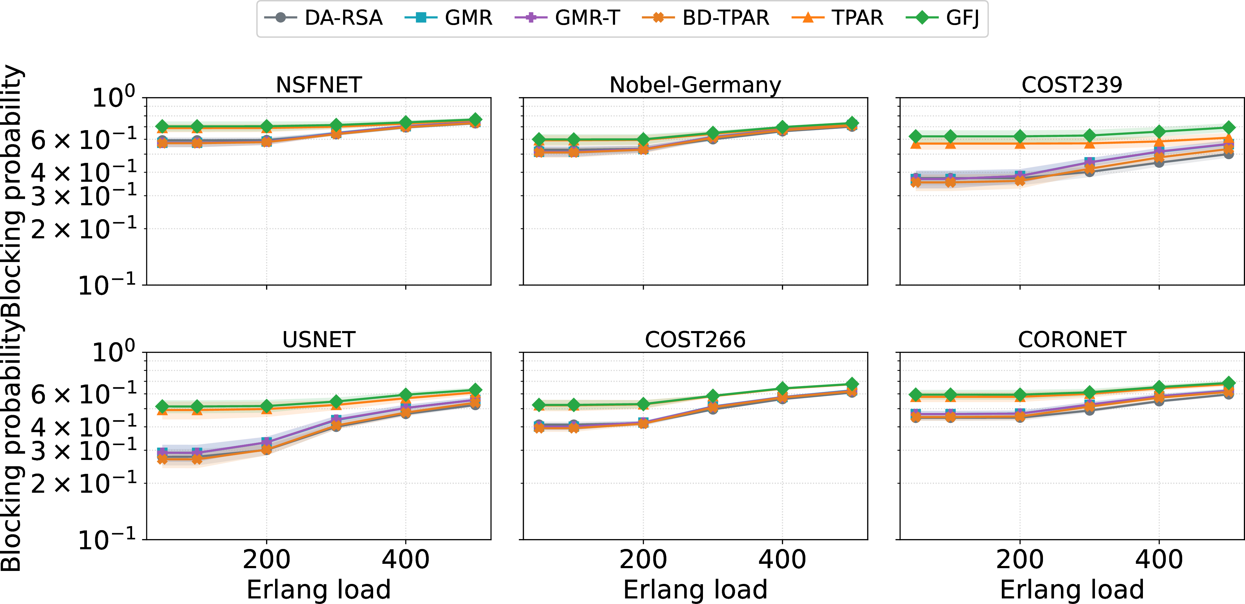
Fig. 2 plots blocking probability against Erlang load at 50% HCF. The six schemes split into three behaviors. The fiber-blind pair (DA-RSA, GMR) gives the lowest blocking baseline; under heavy load (300 Erlang) DA-RSA achieves the minimum point-estimate blocking across all six topologies (0.40 on COST239 up to 0.64 on NSFNET), because its shortest physical paths claim wavelengths most efficiently when spectrum is tight. The middle-ground group (GMR-T, BD-TPAR) tracks DA-RSA closely—their reranking and bounded detour keep path lengths near the shortest feasible option. The transition-minimizers (TPAR, GFJ) block substantially more on every topology because their path selection, constrained to avoid fiber-type crossings, restricts route diversity and raises the latency-asymmetry rejection rate (HC1; Section 5.6). The per-topology differences among the four leading schemes are modest at 95% confidence; the robust effects are TPAR/GFJ’s 20–25% carried-traffic loss and the transition-count reductions, not the small blocking gaps.
5.1.0.1 Why a plain GSNR objective is not enough—and what it pays.
Before crediting the transition-aware schemes, note what a plain GSNR objective achieves on its own—the baseline any explicit scheme must beat. On hybrid topologies the inverse-Extended-GSNR weight favors HCF-heavy paths (\(\gamma_\mathrm{HCF}\!\ll\!\gamma_\mathrm{SMF}\)), which do tend to cross fewer fiber-type boundaries—but only as a weak, topology-dependent side effect. Averaged over the six topologies GMR trims \(N_\text{trans}\) by just \(\sim\)4% relative to DA-RSA (Fig. 3 (b)), and on some it crosses more boundaries than DA-RSA: a GSNR-optimal path is not systematically transition-light. It also pays in spectrum: under wavelength continuity an accepted demand occupies one wavelength on every link of both its working and protection paths, and GMR’s GSNR-optimal routes are on average longer than DA-RSA’s shortest routes, so each acceptance consumes more link-wavelength resources, fewer demands fit concurrently, and carried traffic drops by \(\sim\)4%. This is precisely why an explicit transition term is needed: every scheme further along the progression GMR \(\to\) GMR-T \(\to\) BD-TPAR \(\to\) TPAR \(\to\) GFJ trades more of the same currency—spectrum occupied by longer routes—for a reliable reduction in transitions.
Two observations: carried traffic saturates past a mid-load knee, so the blocking and carried-traffic orderings agree; and latency asymmetry does not differentiate accepted demands because \(\Delta\tau_\text{max}\) clips the tails identically—it matters instead as a blocking mechanism (Section 5.6).
5.2 Modulation mix and carried-traffic cost↩︎
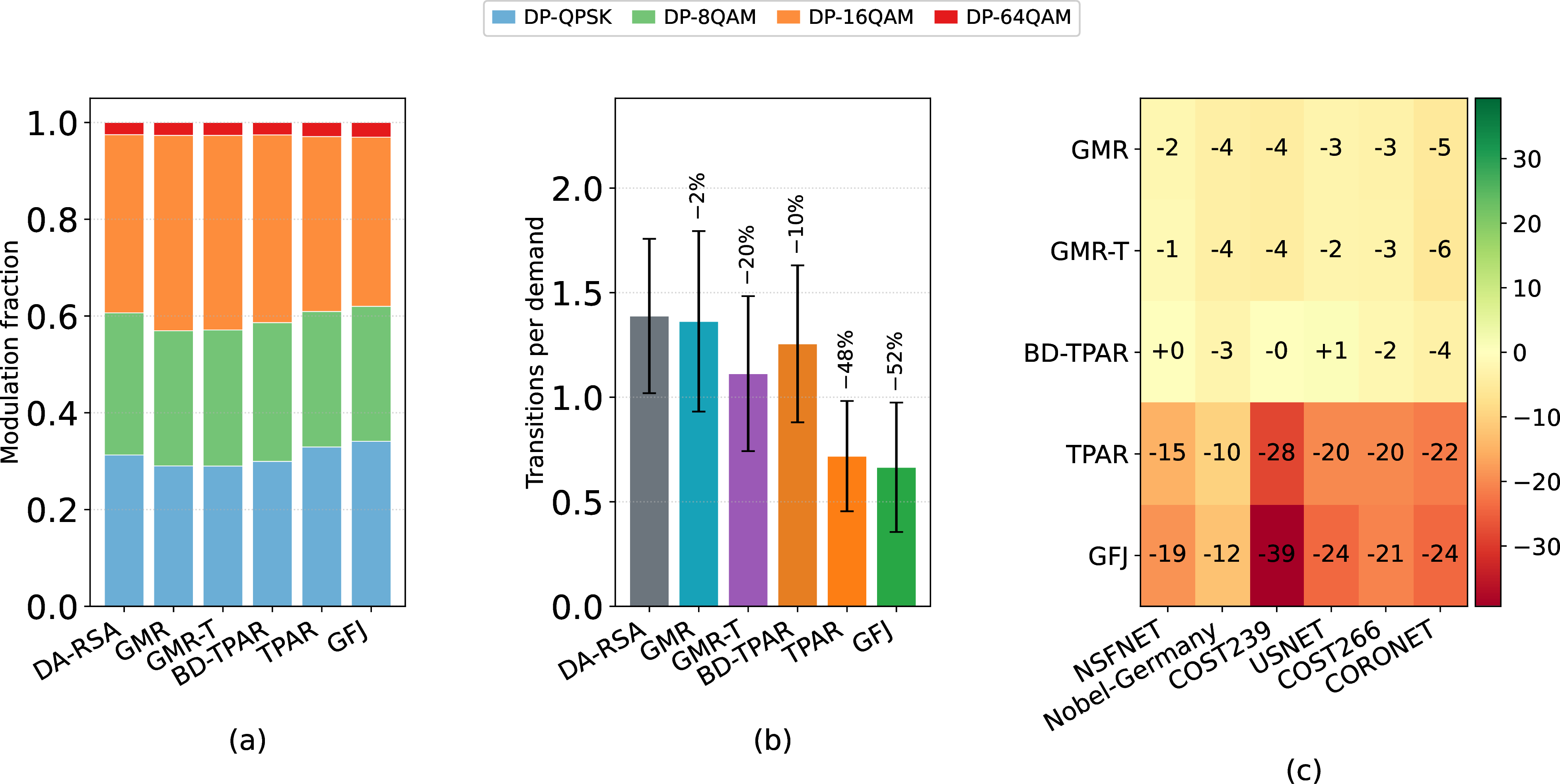
Fig. 3 presents both sides of the central trade-off. Panel (b) shows what each scheme buys: relative to DA-RSA’s 1.39 transitions per accepted demand, GMR-T removes \(\sim\)22%, BD-TPAR \(\sim\)11%, and TPAR/GFJ \(\sim\)50–56%. Panel (c) shows what each pays in carried traffic: BD-TPAR is the closest non-baseline scheme at only \(-1.2\%\), GMR and GMR-T sit near \(-3.5\%\), and only TPAR and GFJ separate sharply at \(-19.2\%\) and \(-23.3\%\). Panel (a) supplies the physical mechanism behind the cost: the minimizers’ longer, detoured paths drop the GSNR margin below the DP-16QAM threshold more often, shifting demands to lower-order formats that carry fewer bits. Taken together: BD-TPAR buys an \(\sim\)11% transition reduction for only a \(\sim\)1% throughput cost, GMR-T buys \(\sim\)22% for \(\sim\)3%, while TPAR/GFJ buy \(\sim\)50–56% at more than an order of magnitude higher cost.
5.3 HCF fraction sweep↩︎

Fig. 4 shows the trade-off versus HCF fraction on CORONET at 300 Erlang. At the boundary fractions (\(p_\text{HCF}\in\{0,1\}\)) the schemes are indistinguishable, since there are no transitions to weight; the spread opens at intermediate fractions. The transition count per accepted demand is zero at the boundaries and peaks at 50% HCF, where the four fiber-blind and middle-ground schemes cluster near 1.3–1.6 (their order within the cluster is within seed noise) while TPAR and GFJ drop to near 0.75.
5.4 HCF deployment pattern: random vs.contiguous↩︎
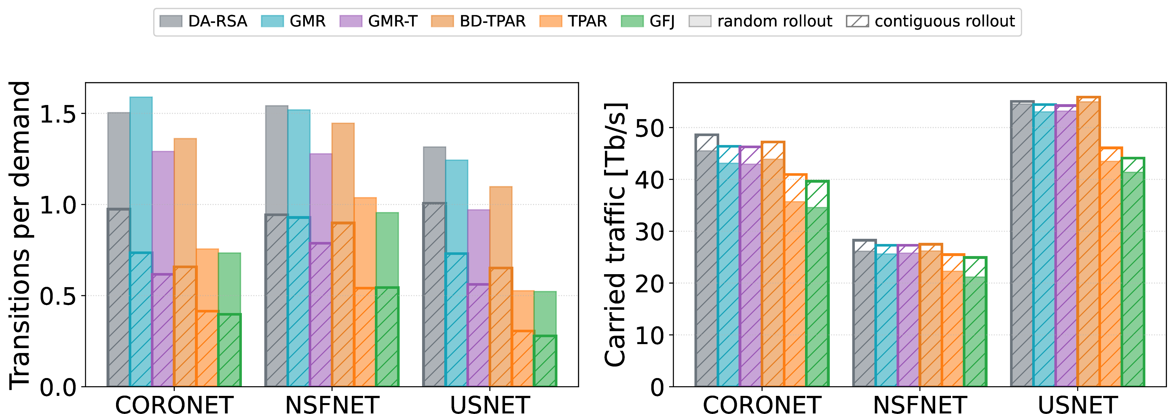
All results so far use uniform-random HCF assignment: the HCF links are a uniformly-random subset of exactly \(\lfloor p_\text{HCF}|E|\rfloor\) edges, drawn without regard to adjacency, so HCF and SMF interleave freely and per-route transition counts are high—a strongly fragmented deployment representative of uncoordinated, opportunistic upgrades. The alternative, contiguous deployment, grows the HCF plant as a single connected cluster by BFS expansion from a seed link (Section 2.1), modeling an operator that upgrades one region at a time; real rollouts are likely closer to this end. Fig. 5 compares the two on three topologies at \(p_\text{HCF}=0.5\) and 300 Erlang. Contiguous deployment cuts the per-demand transition count on every scheme, by 23–54% (mean \(\sim\)42%), and raises carried traffic most where fragmentation hurt most and for the schemes that detour most to avoid transitions—on NSFNET, GFJ gains \(\sim\)18% and TPAR \(\sim\)14%, with three-topology mean gains of \(\sim\)13% (GFJ) and \(\sim\)12% (TPAR) versus only \(\sim\)5% for the leading schemes (DA-RSA, GMR, GMR-T, BD-TPAR). Deployment pattern is thus a throughput-preserving lever reaching transition reductions comparable to TPAR/GFJ’s without their penalty; the transition-minimizers’ advantage shrinks under contiguous rollout, so the decision rule applies most strongly on the fragmented end.
5.5 Per-transition penalty sensitivity↩︎
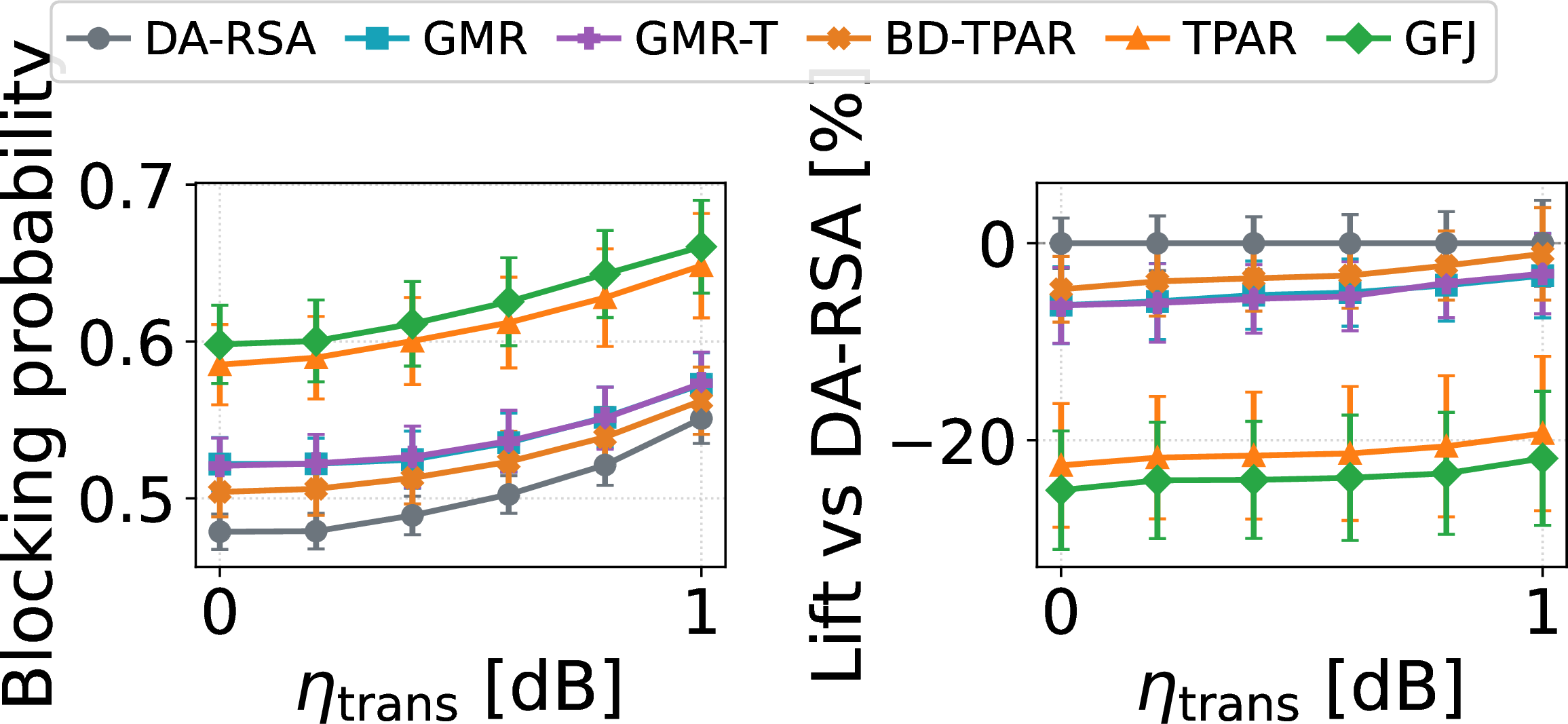
Since \(\eta_\text{trans}\) is a calibrated parameter (Section 2.3), the natural question is whether the conclusions depend on its value. Fig. 6 sweeps it over \([0,1]\) dB on CORONET at 50% HCF and 300 Erlang (360 dedicated trials); they do not. Blocking rises with \(\eta_\text{trans}\) as more candidates cross the modulation cliff—monotonically for every scheme, with DA-RSA nearly flat below \(0.2\) dB (0.479 at both \(0\) and \(0.2\) dB, where the penalty is still too small to prune many candidates) before climbing to 0.551 at \(1\) dB. The ordering is stable across the range: BD-TPAR tracks 2–3 points above DA-RSA and slightly below GMR/GMR-T, its lift over DA-RSA rising from \(-5\%\) toward \(-1\%\) as \(\eta\) grows (its fewer transitions worth more as each costs more), while TPAR/GFJ stay in a \(-19\) to \(-25\%\) band.
5.6 Block-reason decomposition↩︎
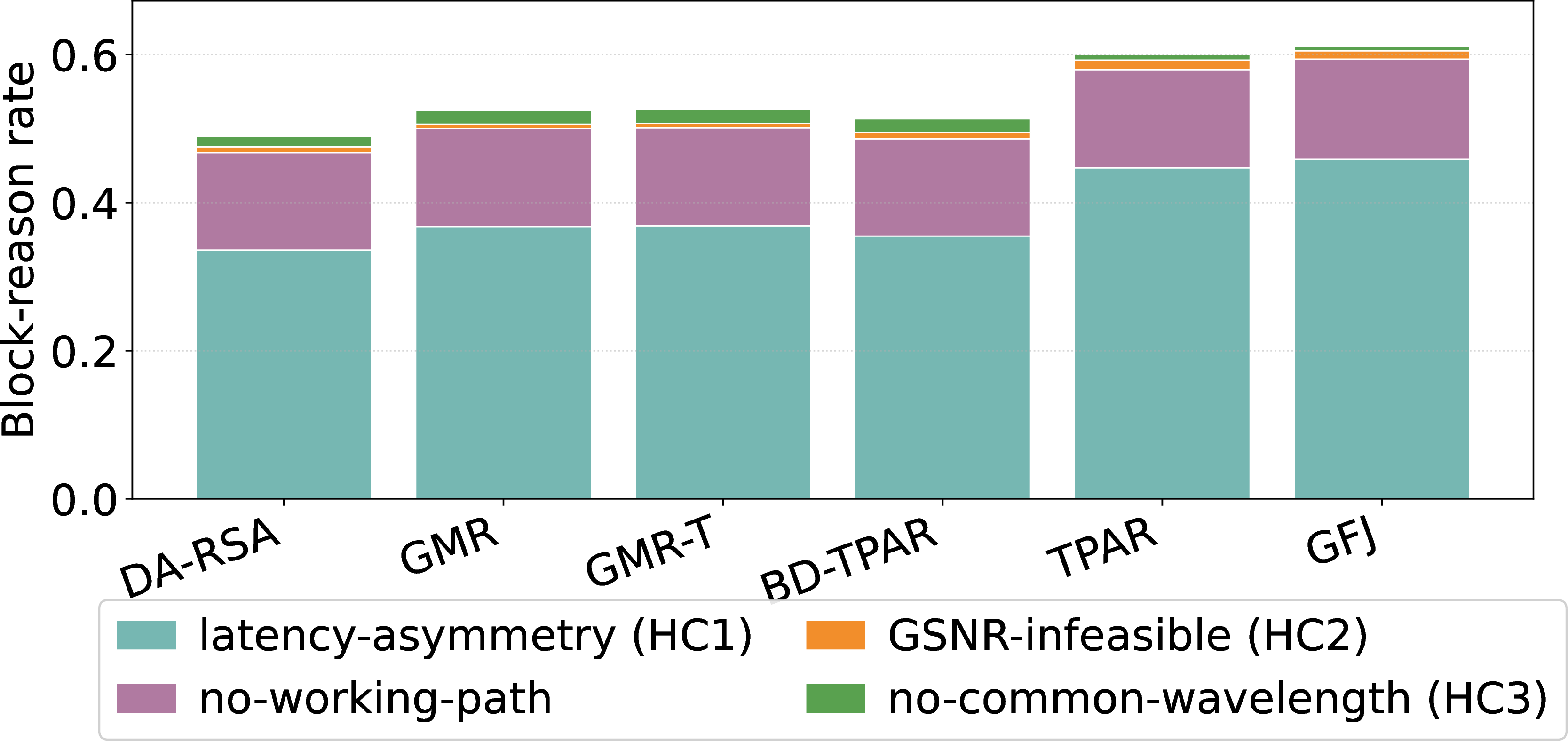
Fig. 7 answers why demands are blocked. Blocking decomposes into four classes summing to the total: latency-asymmetry (HC1—the receiver differential-delay bound of 3 , Section 2.4), no-working-path, GSNR-infeasibility (HC2), and no-common-wavelength (HC3), each demand attributed to the gate at which its preferred route first failed. At 50% HCF / 300 Erlang on CORONET, HC1 dominates every scheme (69–75%), followed by no-working-path (22–27%); spectrum-related rejections are minor (HC3 1–4%, HC2 \(\sim\)1–2%). Demands are lost mainly because no working/backup pair with matched HCF/SMF delays exists—not because wavelengths run out. This also explains the minimizers’ larger traffic loss: avoiding HCF–SMF crossings restricts route diversity and magnifies the delay mismatch, pushing their HC1 share to 74–75% versus \(\sim\)69% for the other four.
5.7 L-band cut with per-channel CO2 absorption↩︎
CO2 absorption in HCF-guided L-band light arises from gas-phase rovibrational lines of the \(2\nu_1{+}\nu_3\) combination band (origin \(\approx190.22\) THz), spaced \(\approx46.4\) GHz apart, each \(\approx1\) GHz wide and reaching \(\approx0.1\) dB/km at the strongest lines [34]. Our 80-channel, 75-GHz L-band grid spans 184.783–190.708 THz (1622–1572 nm). Because 75 GHz is not a multiple of the line spacing, channel centers fall at different offsets from the measured absorption lines [18], [34]. However, a 1-GHz line overlaps only a thin portion of a 64-GBd channel’s \(\approx70\)-GHz occupied bandwidth, so the band-averaged excess loss is far below the line-center peak. Even channel 78, whose center nearly coincides with a strong R-branch line and would incur \(\approx7.4\) dB/100 km under point sampling, experiences only \(\approx0.4\) dB/100 km after band averaging. Most channels experience far less, while channels 0–17 occupy the CO2-quiet region where high-\(J\) lines are Boltzmann-suppressed.
We represent this effect using per-channel GSNR look-up tables, assigning each wavelength slot on every HCF link the effective loss \[\alpha_\text{eff}(\nu_k) =\alpha_\text{HCF} +\bar{\alpha}_{\mathrm{CO}_2}(\nu_k).\] Here, \(\bar{\alpha}_{\mathrm{CO}_2}(\nu_k)\) is a phenomenological comb of 1-GHz-FWHM Lorentzians whose positions and amplitudes are fitted to the measured L-band spectrum of [34] and integrated over the 64-GBd signal bandwidth rather than sampled at the carrier. This is a first-order OSNR treatment: the EDFA compensates the band-averaged excess loss and consequently raises ASE. It is a routing-layer penalty map, not a first-principles line-by-line HITRAN model, and does not capture narrow-band spectral distortion within a channel. GSNR is precomputed for three occupancy states, as in the C-band analysis. Because the profile is non-monotone in channel index, the penalty seen by first-fit assignment depends on load and path length as well as the selected channel.
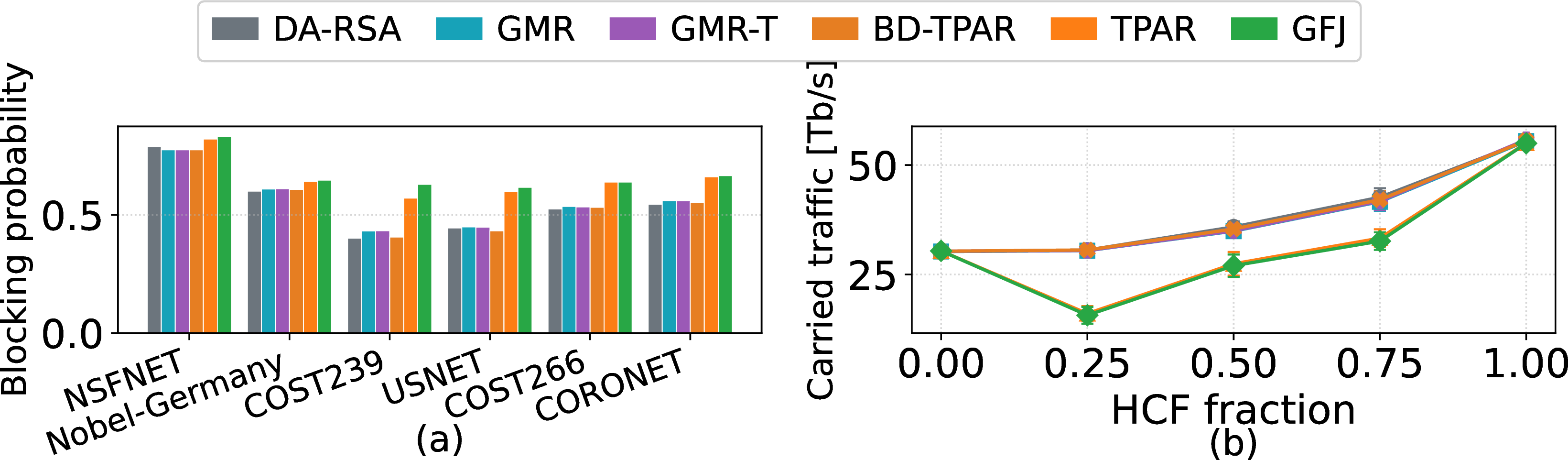
We ran 10,800 trials (6 topologies \(\times\) 5 HCF fractions \(\times\) 6 loads \(\times\) 10 seeds \(\times\) 6 schemes) on the 80-channel L-band grid. Fig. 8 (a) shows that the C-band ordering is preserved at 50% HCF and 300 Erlang: DA-RSA has the lowest blocking on every topology, ranging from 0.40 on COST239 to 0.79 on NSFNET; TPAR and GFJ incur 20–25% mean carried-traffic penalties relative to DA-RSA; and BD-TPAR remains within \(\sim1\%\) of DA-RSA (\(+1.0\%\) by the per-topology mean). The small band-averaged CO2 penalty leaves absolute L-band capacity comparable to the C-band, whereas a point-sampled treatment would instead charge each carrier the full line-center absorption.
Fig. 8 (b) likewise shows that CORONET carried traffic increases monotonically with HCF fraction, from \(\sim30\) Tb/s at the all-SMF endpoint to \(\sim56\) Tb/s at all-HCF for BD-TPAR. The band-averaged gas penalty is therefore too small to offset HCF’s lower loss and near-zero Kerr nonlinearity, making L-band HCF deployment net-beneficial. The residual penalty is confined to channels whose \(\sim70\)-GHz bands overlap dense line clusters. Thus, both the scheme-choice rule and deployment incentive are band-invariant: the scheme ranking is unchanged, and greater HCF deployment helps in both bands.
If the residual penalty must be removed, its known spectral locations make it a spectrum-assignment problem rather than a routing problem: filling quiet channels 0–17 first and line-adjacent channels such as 78 last would recover the remaining few percent without changing path selection. Pre-emphasis and spectral-avoidance capacity maps [18] provide the required per-channel margin bookkeeping, while DSP mitigation using pre-characterized absorption profiles is emerging [25], [34].
5.8 Composite availability with per-splice failure↩︎
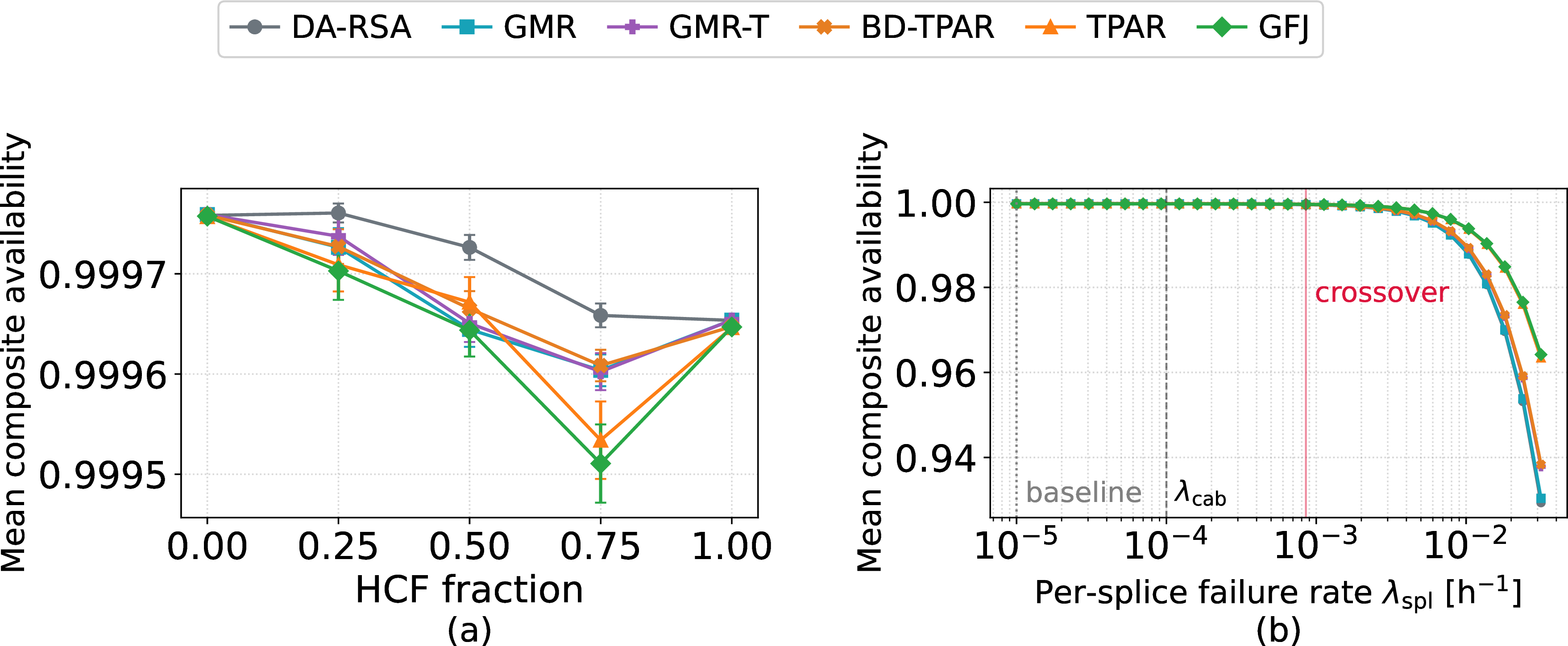
Does transition reduction buy reliability? At our calibration, no. Extra transitions add outage exposure, but composite availability is dominated by the cable-cut and per-channel outage terms, both scaling with working-path length, so the shortest-path scheme (DA-RSA) is the most available by a small margin; all six lie between 0.9996 and 0.9997 at \(p_\text{HCF}=0.5\) (Fig. 9 (a)), none reaching five-nines because the residual per-channel and cable-cut terms cap the 1+1 composite there. Sweeping the per-splice rate over each demand’s captured paths, transition-aware schemes begin to overtake DA-RSA only once \(\lambda_\text{spl}\) reaches approximately \(8.5\times10^{-4}\) h\(^{-1}\) (Fig. 9 (b)); TPAR is the first scheme to cross at this point. This rate is approximately \(85\times\) the already-conservative baseline and implies a splice mean time between failures of about 1200 h, still far above plausible fusion-splice failure rates. Availability is therefore a caution against over-claiming reliability benefits, not an argument for transition-aware routing; the case for transition awareness rests on the operational costs discussed in Section 6.1.
6 Discussion↩︎
6.1 Why a transition has an external cost↩︎
We define \(C_\text{ext}\) as the operator’s per-unit external cost of an HCF\(\leftrightarrow\)SMF transition, in carried-traffic units. It aggregates three operational-incident classes invisible to blocking and throughput. (i) Each interface causes an EDFA gain-target discontinuity: surviving channels see millisecond-scale, multi-decibel transients in cascaded amplifiers [38], [39], consuming optical-signal-to-noise-ratio (OSNR) margin and triggering ROADM retunes. (ii) Each splice is a discrete failure point (rate \(\lambda_\text{spl}\)), so lifetime outage exposure scales with the transition count. (iii) Working and protection paths of different fiber type present different accumulated CD, so hitless switchover requires the transponder DSP to hold equalizer state for both [33] (no public quantification of this specific cost is known to us). We model (i) via \(\eta_\text{trans}\) and (ii) via \(\lambda_\text{spl}\); (iii) is qualitative only. A high \(C_\text{ext}\) reflects an operator whose EDFA-retune budget, MTTR service-level agreements (SLAs), and transponder overhead price transitions heavily; a low \(C_\text{ext}\), one constrained only by spectrum.
6.2 Decision rule↩︎
The rule turns the simulation outputs into a scheme choice in three steps. Step 1: read two numbers per scheme off Fig. 3 (50% HCF, 300 Erlang, six-topology means): the carried-traffic lift over DA-RSA \(w_s\) (panel c) and the mean transitions per accepted demand \(\bar{n}_s\) (panel b). Step 2: set what one transition is worth—the operator’s exchange rate \(\kappa\) (Section 6.1), the percent of carried traffic it would give up to remove one transition per demand (\(\kappa=0\) with no transition costs, large where interface-driven maintenance dominates).
Step 3: pick the scheme on the upper envelope. A scheme’s utility is its throughput lift plus the value of the transitions it saves, \[U_s \;=\; w_s \;+\; \kappa\,\bigl(\bar{n}_\text{DA-RSA}-\bar{n}_s\bigr). \label{eq:utility}\tag{8}\] Because 8 is linear in \(\kappa\), the best scheme at any \(\kappa\) is whichever utility line is highest—the upper envelope of the six lines, read directly off the \((w_s,\bar{n}_s)\) values of Fig. 3. Taking the envelope over all six (not chaining pairwise comparisons) matters: GMR never reaches it, since GMR-T dominates GMR—more transitions saved (\(\bar{n}=1.11\) vs.\(1.36\)) at similar cost—so GMR is never optimal. The remaining schemes partition the \(\kappa\) axis into five regions, delimited by the \(\kappa\) at which adjacent utility lines cross:
\(\kappa < 9\): transitions too cheap to justify any detour – use DA-RSA.
\(9 \le \kappa < 16\): use BD-TPAR (\(\delta=1.2\); GMR fallback) – \(\sim\)11% fewer transitions at almost no throughput cost.
\(16 \le \kappa < 40\): use GMR-T – a larger \(\sim\)22% transition cut for \(\sim\)3% throughput.
\(40 \le \kappa < 77\): use TPAR.
\(\kappa \ge 77\): use GFJ.
Concretely: an operator willing to give up 1% of carried traffic to remove 0.1 transitions per demand sits at \(\kappa=1/0.1=10\) (BD-TPAR); one willing to give up 3% for the same 0.1 sits at \(\kappa=30\) (GMR-T).
Two qualifiers bracket the rule. First, it matters most under fragmented rollout. The exchange rate \(\kappa\) is a property of the operator’s cost structure, not the topology; what contiguous deployment changes is the transition-savings term \((\bar{n}_\text{DA-RSA}-\bar{n}_s)\) multiplying \(\kappa\) in 8 . Removing \(\sim\)40% of transitions structurally (Section 5.4) shrinks that term for every scheme, so the utility advantage of transition-aware routing collapses toward zero even at large \(\kappa\). Second, the breakpoints are heavy-load numbers (\(w_s\) at 300 Erlang). At light load (50–100 Erlang) the middle-ground schemes edge ahead of DA-RSA (\(+2\) to \(+3\%\)), their transition-light paths keeping more GSNR margin while spectrum is plentiful, so below the blocking knee they are safe at any \(\kappa\). The TPAR/GFJ penalty, however, persists at all loads (\(-23\) to \(-27\%\)) because it stems from latency-asymmetry rejection, not spectrum contention; the \(\kappa\gtrsim40\) gate applies at any load.
7 Conclusion↩︎
We compared six protected routing schemes on a common event-driven simulator with an IMI-augmented GN model and a calibrated per-transition GSNR penalty; the middle-ground schemes introduced here—GMR-T and BD-TPAR—fill the gap between fiber-blind baselines and aggressive minimizers. The preferred scheme depends on load regime and operator cost structure, not on a universal ranking. Under heavy load, latency-asymmetry rejection (HC1) binds and DA-RSA is the throughput champion; BD-TPAR is the closest non-baseline scheme at only \(-1.2\%\) cost for \(\sim\)11% fewer transitions, and GMR-T buys \(\sim\)22% fewer for \(\sim\)3%. Aggressive minimizers (TPAR, GFJ) halve transitions but cost 20–25% of carried traffic, justified only when the operator’s transition-to-throughput exchange rate exceeds \(\kappa\approx40\) (Section 6.2). The ordering also holds in the L-band, where a band-averaged CO2 penalty leaves HCF net-beneficial. Contiguous HCF rollout is the strongest lever (23–54% fewer transitions, higher carried traffic); routing adds value on top, most under fragmented rollout. These results replace “which scheme is best?” with “what cost structure does the operator carry?”
No funding received for this work. Generative AI was used for language editing.
The authors declare no conflicts of interest.
Data underlying the results presented in this paper are not publicly available at this time but may be obtained from the authors upon reasonable request.
References↩︎
The acronym “GFJ” is the name we use in this work for the GSNR/Fiber-transition Joint formulation; it is not standard terminology.↩︎