A structure-preserving numerical method for the compressible Resistive-Hall-MHD system
July 15, 2026
Abstract
In this paper, we present a structure-preserving method for the compressible resistive Hall-magnetohydrodynamics (MHD) model. The differential operator is split into two parts: a hydrodynamic part consisting of the compressible Euler equations, and a magnetic part consisting of a system coupling the Lorentz force and the induction equation. The method uses continuous Lagrange elements for the Euler part and a curl-conforming finite element space for the magnetic part. The hydrodynamic part preserves the positivity of the density and internal energy, the conservation of total energy, and the minimum principle for the specific entropy. Owing to the choice of finite elements, the magnetic part preserves the divergence involution constraint. The fluid part is solved using explicit strong-stability-preserving Runge–Kutta (SSP-RK) methods, whereas the magnetic part is solved by Crank-Nicholson method, which requires using Newton’s method. Coercivity estimates for the Jacobian of the corresponding Newton iteration are presented. We introduce a high-order artificial resistivity to improve the conditioning of the nonlinear residual and the invertibility of the Jacobian. Several challenging benchmarks, including a smooth whistler wave, the Orszag–Tang vortex for comparing resistive MHD with resistive Hall-MHD, and a magnetic reconnection problem, are solved to validate the robustness and accuracy of the method.
Resistive Hall MHD ,structure preserving ,invariant domain ,involution constraints ,energy-stability ,magnetic reconnection
1 Introduction↩︎
In this work we consider the numerical solution of the compressible Hall-MHD system: \[\tag{1} \begin{align} \partial_t \rho + \diver{} \mom &= 0 \, ,\\ \partial_t \mom + \diver{} (\rho^{-1}\mom \mom^\transp + \mathbb{I} p) &= \mu \curl{}\Hfield \times \Hfield \\ \tag{2} \partial_t \totme + \diver{}\big(\tfrac{\mom}{\rho} (\totme + p) \big) &= \mu (\curl{}\Hfield \times \Hfield)\cdot \tfrac{\mom}{\rho} + \resist |\curl{}\Hfield|^2 \, , \\ \tag{3} \partial_t \Hfield - \curl{}(\tfrac{\mom}{\rho} \times \Hfield) &= - \curl{}(\tfrac{\resist}{\mu} \curl{}\Hfield + \tfrac{d_i}{\rho} \curl{}\Hfield \times \Hfield) \end{align}\] where \(\rho \in \mathbb{R}\) is the density, \(\mom \in \mathbb{R}^3\) is the momentum, \(\mathbb{I} \in \mathbb{R}^{3 \times 3}\) is the identity matrix, \(\totme \in \mathbb{R}\) is the total mechanical energy, and \(\Hfield \in \mathbb{R}^3\) is the magnetic field. Here the constant \(\resist\) is the resistivity while \(d_i = \frac{m_i}{q_i}\): the constant \(m_i > 0\) is the specific ion mass while \(q_i > 0\) is the specific ion charge, see for instance [1]. The term \(\curl{}(\resist \curl{}\Hfield)\) in the right hand side of 3 is resistive term, while the term \(\curl{}(\tfrac{d_i}{\rho} \curl{}\Hfield \times \Hfield)\) is the Hall term. Note that resistive effects introduce the source of heat \(\resist |\curl{}\Hfield|^2\) in the right hand side of 2 .
The MHD equations are widely used in astrophysics applications as well as in nuclear fusion research [2], [3], where it is used to study instabilities in plasma confinement [4], [5]. The MHD system can be understood as a formal asymptotic limit of the two-fluid Euler-Maxwell model. More precisely it is the limit obtained under the assumptions of infinite speed of light (equivalently, zero electric permittivity, that is \(\epsilon_0 \rightarrow 0^+\)) and zero electron mass. Most frequently, the Hall term is neglected during the derivation of the ideal MHD model. The importance of the Hall term was first pointed out by James Lighthill in [6]. Derivations of the Hall-MHD system can be found in [7], [8]. Since the early 2000s there has been a growing body of scientific literature indicating that Resistive and Hall terms are fundamental to reproduce magnetic reconnection rates [9]–[12] observed in practice.
Numerical solutions of the MHD system are vital to predict phenomena in various scientific fields such as plasma physics and astrophysics. Furthermore, when performing numerical simulations of the MHD system, it is crucial to ensure the preservation of essential structure of the solution, such as positivity properties, conservation of total energy, entropy-dissipation, and involution constraints. For instance, the works of [13]–[16], along with references provided therein, represent just a subset of the comprehensive research dedicated to achieving positivity-preserving approximations for the compressible ideal MHD system.
Another very important property preserved by the ideal-MHD and Resistive-Hall-MHD systems is the involution constraint of the magnetic field, that is, the invariance of the magnetic field’s divergence. Time-invariance of the magnetic field implies that if the magnetic field is zero at initial time, then, it should remain zero for all time. Without making any claim of completeness, some references advancing numerical techniques that preserve some aspect of the involution (e.g. locally divergence-free and divergence cleaning methods) are [17]–[20].
Overall, the literature on structure preserving methods for the ideal compressible MHD system is reasonably developed. On the other hand, the list mathematical references1 advancing numerical schemes for the compressible Resistive-Hall-MHD system is noticeably small. A fairly complete list of references obtained from MathSciNet database, with specific focus on compressible Resistive-Hall-MHD, is [21]–[27]. To the best of our knowledge, there is no literature with a focus on structure preservation of the compressible Resistive-Hall-MHD system.
The development of numerical methods for the MHD systems is inextricably associated to the divergence formulation. The divergence formulation of the ideal MHD system offers a few challenges that are hard to ignore. Among them, the divergence formulation is not Galilean invariant, it is not symmetrizable, and its Jacobian is defective (it does not possess a full set of eigenvectors). From the purely computational perspective, the Riemann problem of the ideal MHD in divergence form is not well defined unless the condition \([\![\Bfield]\!]\cdot\normal = 0\) holds across discontinuity surfaces [28]. Computationally, some of these problems may be alleviated with the inclusion of modifications of the scheme, for instance, with the use of constraint transport techniques, see for instance [29] and references therein.
Regarding the existence of solutions for compressible Hall-MHD models very little is known. An extensive literature search reveals that most, if not all, the Analysis literature is limited to short-time existence of strong solutions [30]–[34]. Notably, to the best of our knowledge, there are no existence results for the compressible Hall-MHD model without resistivity. On the other hand, the role of resistivity, for the incompressible Hall-MHD model, is well understood: resistivity is fundamental to achieve well-posedness of the incompressible Hall-MHD model. In a series of highly cited publications [35]–[37] it was proven that the incompressible Hall-MHD model without resistivity is ill-posed. Based on this record of Analysis results, it may be reasonable to assume that resistivity is fundamental to guarantee well-posedness of the compressible Hall-MHD model as well.
The current work is a continuation of the ideas advanced in [38]. In that work, the authors advanced a proof of the minimum principle of the specific entropy as well as entropy-dissipation inequalities that do not involve viscous regularization of the magnetic field. These results indicate that the ideal MHD is not a conservation law in the vanishing-viscosity sense of [39]–[41]. Inspired by this result, we developed a numerical scheme that decomposes the ideal MHD system into Euler’s equation and a purely Hamiltonian PDE that couples the Lorentz force and the induction equation. Such scheme is capable of preserving positivity properties, total energy, involution constraints, and entropy-dissipation inequalities with no divergence-cleaning or related tools. Most importantly, the induction equation is not stabilized in any form or fashion: which is entirely consistent with the vanishing-viscosity argument.
In this paper, we extend the ideas of [38] to the case of the Resistive-Hall-MHD model. We develop a new scheme that preserves positivity of the density, positivity of the internal energy, total mechanical energy, minimum principle of the specific entropy. We also prove that the scheme preserves entropy-dissipation inequalities if the numerical method used to solve Euler’s system preserves such a property. The scheme is semi-implicit: Euler’s system is advanced explicitly, while the source system consisting of the Lorentz force coupled to the induction equation is advanced in a time-implicit fashion.
One of the most important differences between the present work and [38] is the behaviour of nonlinear solvers. In our previous work we used Newton’s method to solve the nonlinear residual associated to the coupled system involving Lorentz force and the induction equation. In that work, nonlinear performance turned out to be exceptional across several tests and mesh types: Newton’s solver never exceeded 4 iterations per time-step. The addition of the Resistive term is benign and does not change the behaviour/performance of Newton’s scheme. However, the addition of the Hall terms is rather delicate. Our initial computations for the Resistive-Hall-MHD system, using uniform structured meshes, delivered comparable performance along the lines of at most 4-5 Newton iterations per time step. However, such results did not translate to other mesh types. Nonlinear solver performance turned out to be rather inconsistent across several types of meshes: either too many Newton iterations were required or the Jacobian was severely ill-conditioned. This is not strictly speaking a defect of the scheme, but rather a problem associated with our choice of nonlinear solver. Since we were unwilling to give up Newton’s method2 and its second-order convergence, we decided to modify the scheme. Coercivity analysis of the Jacobian reveals a loss of invertibility whenever the electron speed is too large. Therefore, we devised an artificial resistivity for the induction equation that improves well-posedness of the Jacobian, thereby stabilizing the behaviour of nonlinear Newton iterations.
One of the most important aspects of scientific computing is Verification and Validation [42]. Generally speaking, verification consists in checking that the method is convergent. The standard quantitative test is computation of convergence rates (or log-log plots) using exact solutions3. However, exact analytical solutions for the compressible-Resistive-MHD model are not available at this point in time. This makes quantitative evaluation of the scheme very difficult. On the other hand, qualitative tests are just limited to graphical comparison. Again, given the extremely rarefied body of literature on this model, there are just a few meaningful computational results, most of which use very coarse meshes to be considered reference results. For instance, with the exception of [27], pretty much every computation of the Resistive-Hall-MHD model available in the literature uses 128\(\times\)128 cells for the GEM challenge problem.
In this regard, one of our most important contributions is the development of both quantitative tests and reference computational results. We present a quantitative test consisting of a smooth-traveling wave, in the linear resistive regime that allows us to verify some aspects of the accuracy of the method. We illustrate the computation of the GEM challenge with resolutions of up to 1024\(\times\)1024 elements. Our long-term goal is to make the corresponding data available to the wider scientific community. We also advance direct comparisons of Resistive-MHD vs Resistive-Hall-MHD with Orzag-Tang vortex test using resolutions of up to 724\(\times\)724 cells. Finally, to the best of our knowledge, there are no computations of the Resistive-Hall-MHD model using unstructured meshes, with most, if not all results using structured cartesian meshes. It is well-known that most numerical methods use to solve hyperbolic-like problems are very sensitive to mesh-imprint artifacts. In this work, we present a series of results using structured isotropic meshes, structured anisotropic, fully unstructured quasi-uniform meshes, and criss-cross meshes, showing that our method delivers comparable results regardless of the choice of mesh.
The paper is organized as follows: in Section 2 we present a splitting of the differential operator 1 , prove the properties preserved by each operator and show that the splitting is compatible with the sequential preservation of such properties. In Section 3.1 we summarize the notation related to the space discretization. In Section 3.2 we provide the space and time discretization of the source-system associated to the Lorentz force and the induction equation (containing the ideal, Hall, and resistive terms). The main theoretical results of this scheme are independent of the choice of numerical scheme used to solve Euler’s system. Therefore, in Section 3.3 we outline the main assumptions made about the hyperbolic solver. The precise choice of hyperbolic solver used for all our computations is described in Appendix B of our previous work [38]. In Section 3.4 we elaborate our motivations for the development of an artificial viscosity. In Section 3.5 we make precise the artificial viscosity used for all our computations. In Section 3.6 we provide an algorithmic summary of the whole operator splitting scheme. In Section 4 we present our numerical results.
Finally, we mention that this paper has three appendices. 6 contains a summary of thermodynamic properties which are used in the context of Sections 1 and 3.2. 7 contains the derivation of the Jacobian and its coercivity analysis: this appendix and its contents play a very important role in this paper. 8 describes the implementation of the 2.5-space dimensions implementation.
2 Splitting of the differential operator↩︎
We start by splitting 1 into two differential operators \[\begin{align} \label{OperatorOne} \text{Operator }\#1 \left\{ \begin{aligned} \partial_t \rho + \diver{} \mom &= 0 \, ,\\ \partial_t \mom + \diver{} (\rho^{-1}\mom \mom^\transp + \mathbb{I} p) &= \bzero \\ \partial_t \totme + \diver{}\big(\tfrac{\mom}{\rho} (\totme + p) \big) &= 0 \, , \\ \partial_t \Hfield &= \bzero \end{aligned} \right. \end{align}\tag{4}\] and \[\begin{align} \label{OperatorTwo} \text{Operator }\#2 \left\{ \begin{aligned} \partial_t \rho &= 0 \, ,\\ \partial_t \mom - \mu \curl{}\Hfield \times \Hfield &= \bzero \\ \partial_t \totme - \mu (\curl{}\Hfield \times \Hfield)\cdot \tfrac{\mom}{\rho} - \resist |\curl{}\Hfield|^2 &= 0\\ \partial_t \Hfield - \curl{}(\tfrac{\mom}{\rho} \times \Hfield) + \curl{}(\tfrac{\resist}{\mu} \curl{}\Hfield + \tfrac{d_i}{\rho} \curl{}\Hfield \times \Hfield) &= \bzero \end{aligned} \right. \end{align}\tag{5}\] We briefly discuss the properties preserved by each operator. We will assume that the pressure is computed from a complete Equation of State (EOS) as described by 54 . In particular, we assume that the EOS satisfies the assumptions 55 and 56 , see 6 for more details. In Section 3 we outline the development of numerical schemes that preserve such properties in the fully-discrete setting.
Let \(t_1 < t_2\), consider the time interval \([t_1, t_2]\) and that \(\mom\cdot\normal = 0\) in the entirety of the boundary \(\partial\domain\), compactly supported initial data, and that \(t_2 - t_1\) is small enough such that no wave reaches the boundary for any \(t \in [t_1, t_2]\). Alternatively, assume periodic boundary conditions. Then, the solution operator 4 satisfies the following properties: \[\begin{align} \label{ConsPropGlobal} \begin{aligned} \int_{\Omega} \rho(\xcoord, t_2) \dx = \int_{\Omega} \rho(\xcoord, t_1)\dx \;, \;\; \int_{\Omega} \mom(\xcoord, t_2) \dx = \int_{\Omega} \mom(\xcoord, t_1)\dx \\ \int_{\Omega} \totme(\xcoord, t_2) \dx = \int_{\Omega} \totme(\xcoord, t_1)\dx \;, \;\; \int_{\Omega} \Hfield(\xcoord, t_2) \dx = \int_{\Omega} \Hfield(\xcoord, t_1)\dx \end{aligned} \end{align}\tag{6}\] Note that the conservation properties on the magnetic field follow trivially since \(\Hfield(\xcoord, t_2)\) \(\equiv \Hfield(\xcoord, t_1)\) in the context of Operator #1. Therefore, we also have that \[\begin{align} \label{OpOneTotalNRG} \int_{\Omega} \totme(\xcoord, t_2) + \tfrac{\mu}{2} |\Hfield(\xcoord, t_2)|^2\dx = \int_{\Omega} \totme(\xcoord, t_1) + \tfrac{\mu}{2} |\Hfield(\xcoord, t_1)|^2\dx \end{align}\tag{7}\]
Regarding pointwise properties: we have that \[\begin{align} \label{EulerPositDens} \inf_{(\xcoord,t) \in \Omega \times [t_1,t_2]} \rho(\xcoord,t) \geq 0 \, , \end{align}\tag{8}\] provided that the initial data \(\rho(\xcoord, t_1) \geq 0\) for all \(\xcoord \in \Omega\), for the specific entropy we have that: \[\begin{align} \inf_{\xcoord \in \Omega } s(\rho(\xcoord, t_2),e(\state(\xcoord, t_2)) \geq \inf_{\xcoord \in \Omega} s(\rho(\xcoord, t_1),e(\state(\xcoord, t_1)) \end{align}\] and the mathematical entropy satisfies \[\begin{align} \label{EntDissipPointwise} \partial_t \eta(\state) + \diver{} \mathbb{q}(\state) \leq 0 \;\; \text{for all } (\xcoord, t) \in \domain \times [t_1, t_2] \end{align}\tag{9}\] where \(\{\eta, \mathbb{q}\} = \{- \rho s, -\mom s\}\) is the entropy-flux pair. Integration on \(\Omega\) of the pointwise estimate 9 naturally leads to the inequality: \[\begin{align} \int_{\domain} \eta(\state(\xcoord, t_2)) \dx \leq \int_{\domain} \eta(\state(\xcoord, t_1)) \dx \end{align}\]
We do not advance a proof of this proposition since it is a recollection of well-known results about Euler’s system. Conservation properties 6 are just a consequence of the divergence theorem. The non-negativity of the
density 8 is proved, for instance, in [43]. For the specific case of the ideal gas equation of state, the minimum
principle of the specific entropy was proved for the first time in [44]. For the case of (arbitrary) thermodynamically stable4 equations of state, a proof of the minimum principle of the specific entropy can be found in [43]. The entropy-dissipation inequality 9 is a consequence of the vanishing viscosity principle and the convexity of \(\eta(\state)\) with respect to
\(\state = [\rho, \mom,
\totme]^\transp\), see for instance [45].
The following proposition makes significant use the thermodynamics summary in 6. The reader unfamiliar with the basics of thermodynamics is encouraged to read the Appendix before reading Proposition [prop:op95one95prop].
Let \(t_1 < t_2\), assume that the initial data is such that \[\label{OpTwoPointAss} \begin{gather} \rho(\xcoord, t_1) > 0 \; , \;\; e(\xcoord, t_1) := (\totme - \tfrac{1}{2}\rho |\vel|^2)(\xcoord, t_1) > 0 \\ \;\;\text{and} \;\; \theta(\rho(\xcoord, t_1), e(\xcoord, t_1)) := \big[\tfrac{\partial}{\partial e} s(\tfrac{1}{\rho(\xcoord, t_1)}, e(\xcoord, t_1))\big]^{-1} > 0 \;\;\text{for all }\xcoord \in \domain , \end{gather}\qquad{(1)}\] here \(\theta(\rho(\xcoord, t_1), e(\xcoord, t_1))\) is the temperature at time \(t_1\). Then, Operator #2 as described in 5 , preserves the following properties: \[\begin{align} & \begin{aligned}\tag{10} & \int_{\domain} (\tfrac{1}{2}\rho|\vel|^2 + \tfrac{\mu}{2}|\Hfield|^2)(\xcoord, t_2) \dx \\ & \;\;\;+ \int_{t_1}^{t_2} \int_{\partial\domain} \Big( \resist \curl{}\Hfield - \mu (\vel \times \Hfield) + \tfrac{\mu d_i}{\rho} \curl{}\Hfield \times \Hfield \Big) \cdot (\Hfield \times \normal) \ds \mathrm{d}t \\ & \;\;\;= \int_{\domain} (\tfrac{1}{2}\rho|\vel|^2 + \tfrac{\mu}{2}|\Hfield|^2)(\xcoord, t_1) \dx - \int_{t_1}^{t_2} \int_{\domain} \resist |\curl{}\Hfield|^2 \dx \mathrm{d}t \end{aligned} \\ \tag{11} &(\totme - \tfrac{1}{2} \rho|\vel|^2)(\xcoord, t_2) = (\totme - \tfrac{1}{2} \rho|\vel|^2)(\xcoord, t_1) + \int_{t_1}^{t_2} \resist |\curl{}\current|^2 \mathrm{d}t \\ \tag{12} &\theta(\rho(\xcoord, t_2), e(\xcoord, t_2)) \geq \theta(\rho(\xcoord, t_1), e(\xcoord, t_1)) \\ \tag{13} &s(\rho(\xcoord, t_2), e(\xcoord, t_2)) \geq s(\rho(\xcoord, t_1), e(\xcoord, t_1)) \\ \tag{14} &\eta(\rho(\xcoord, t_2), e(\xcoord, t_2)) \leq \eta(\rho(\xcoord, t_1), e(\xcoord, t_1)) \end{align}\] Note that properties 11 14 are pointwise properties, that is, they hold for every \(\xcoord \in \domain\).
Proof. We start by noting that since \(\partial_t \rho = 0\), Operator #2 can be rewritten as: \[\begin{align} \tag{15} \rho \partial_t \vel - \mu \curl{}\Hfield \times \Hfield &= \bzero \\ \tag{16} \partial_t \totme - \mu (\curl{}\Hfield \times \Hfield)\cdot \vel - \resist |\curl{}\Hfield|^2 &= 0\\ \tag{17} \partial_t \Hfield + \curl{}(\tfrac{\resist}{\mu} \curl{}\Hfield - \vel \times \Hfield + \tfrac{d_i}{\rho} \curl{}\Hfield \times \Hfield) &= \bzero \end{align}\] Now, we multiply 15 by \(\vel\) and 17 by \(\mu \Hfield\) and integrate in space to obtain: \[\begin{align} \label{SourceMomEnergy} \int_{\domain} \partial_t \big(\tfrac{1}{2}\rho |\vel|^2\big) - \mu (\curl{}\Hfield \times \Hfield)\cdot \vel \dx &= \bzero \\ \nonumber \int_{\domain} \tfrac{1}{2} \mu |\Hfield|^2 + \curl{}(\resist \curl{}\Hfield - \mu \vel \times \Hfield + \tfrac{\mu d_i}{\rho} \curl{}\Hfield \times \Hfield)\cdot\Hfield \dx &= \bzero \, . \end{align}\tag{18}\] Now, integrating by parts this last equation we obtain: \[\begin{align} \label{sourceIntbyParts} \begin{aligned} &\int_{\domain} \tfrac{1}{2} \mu |\Hfield|^2 + (\resist \curl{}\Hfield - \mu \vel \times \Hfield + \tfrac{\mu d_i}{\rho} \curl{}\Hfield \times \Hfield)\cdot\curl{}\Hfield \dx \\ &\;\;\; + \int_{\partial\domain} (\resist \curl{}\Hfield - \mu \vel \times \Hfield + \tfrac{\mu d_i}{\rho} \curl{}\Hfield \times \Hfield) \cdot (\Hfield \times \normal) \ds = \bzero \, , \end{aligned} \end{align}\tag{19}\] adding 18 to 19 we obtain: \[\begin{align} \begin{aligned} & \tfrac{\partial}{\partial t} \int_{\domain} \tfrac{1}{2}\rho|\vel|^2 + \tfrac{\mu}{2}|\Hfield|^2 \dx \\ & \;\;+ \int_{\partial\domain} \Big( \resist \curl{}\Hfield - \mu (\vel \times \Hfield) + \tfrac{\mu d_i}{\rho} \curl{}\Hfield \times \Hfield \Big) \cdot (\Hfield \times \normal) \ds = - \int_{\domain} \resist |\curl{}\Hfield|^2 \dx \\ \end{aligned} \end{align}\] Integrating this expression in time between time \(t_1\) and \(t_2\) then 10 follows. Now we multiply 15 by \(\vel\) and subtract the result from 16 to obtain \[\begin{align} \label{Op2consEnergyII} \tfrac{\partial}{\partial t} \big(\totme - \tfrac{1}{2} \rho|\vel|^2 \big) = \resist |\curl{}\current|^2 . \end{align}\tag{20}\] Integrating 20 in time between time \(t_1\) and \(t_2\) then 11 follows. Since \(\partial_t \rho = 0\) in the context of Operator #2, we can divide 20 by \(\rho\) to obtain: \[\begin{align} \label{Op2consEnergyIII} \tfrac{\partial e}{\partial t} = \tfrac{\partial}{\partial t} \big(\tfrac{\totme}{\rho} - \tfrac{1}{2}|\vel|^2 \big) = \tfrac{\resist}{\rho} |\curl{}\current|^2 \, , \end{align}\tag{21}\] therefore the specific internal energy can only increase during the evolution of Operator #2. Since \(\partial_t \rho = 0\) and \(\frac{\partial \theta}{\partial e} \geq 0\), see convexity Assumption 56 57 , then 21 implies that the temperature \(\theta\) can only increase during the evolution of Operator #2. More precisely, using the fundamental theorem of calculus, the chain rule, the thermodynamic relationships in 54 , and identity 21 we have that: \[\begin{align} \label{PositThetaProof} \begin{aligned} &\theta(\rho(\xcoord, t_2), e(\xcoord, t_2)) - \theta(\rho(\xcoord, t_1), e(\xcoord, t_1)) \\ & \;\;\;= \int_{t_1}^{t_2} \partial_t \theta(\rho,e) \mathrm{d}t = \int_{t_1}^{t_2} \frac{\partial \theta}{\partial e} \frac{\partial e}{\partial t}\mathrm{d}t \\ & \;\;\;= \int_{t_1}^{t_2} \frac{\partial }{\partial e} \Big[\frac{\partial s}{\partial e}\Big]^{-1} \frac{\partial e}{\partial t}\mathrm{d}t = - \int_{t_1}^{t_2} \Big[\frac{\partial s}{\partial e}\Big]^{-2} \frac{\partial^2 s}{\partial^2 e} \frac{\partial e}{\partial t}\mathrm{d}t \\ &\;\;\;= - \int_{t_1}^{t_2} \theta^2 \frac{\partial^2 s}{\partial^2 e} \frac{\resist}{\rho} |\curl{}\current|^2 \mathrm{d}t \geq 0 \, \;\; \; \text{for all }\xcoord \in \domain \end{aligned} \end{align}\tag{22}\] where the last inequality follows from the convexity assumption \(\frac{\partial^2 s}{\partial^2 e} \leq 0\), see 57 . Combining assumption ?? with 22 establishes that \(\theta(\rho(\xcoord, t), e(\state(\xcoord, t)))\) can only take strictly positive values in the interval \([t_1, t_2]\). Similarly, since \(\partial_t \rho = 0\) in the context of Operator #2, using the thermodynamic relationship \(\tfrac{\partial s}{\partial e} = \frac{1}{\theta}\), and identity 21 we obtain: \[\begin{align} \label{sminProof} \begin{aligned} & s(\rho(\xcoord, t_2), e(\state(\xcoord, t_2))) - s(\rho(\xcoord, t_1), e(\state(\xcoord, t_1))) \\ & \;\;\;= \int_{t_1}^{t_2} \partial_t s(\rho,e) \mathrm{d}t = \int_{t_1}^{t_2} \frac{\partial s}{\partial e} \frac{\partial e}{\partial t} \mathrm{d}t = \int_{t_1}^{t_2} \frac{1}{\theta} \frac{\resist}{\rho} |\curl{}\current|^2 \mathrm{d}t \geq 0 \end{aligned} \end{align}\tag{23}\] where the inequality follows from the fact that \(\theta\) can only take positive values in the interval \([t_1, t_2]\). Therefore 23 leads to the proof of 13 . Now, reorganizing 23 and multiplying both sides of the equality by \(- \rho(\xcoord, t_1)\) we obtain: \[\begin{align} \label{etaDissPointI} \begin{aligned} & - \rho(\xcoord, t_1) s(\rho(\xcoord, t_2), e(\state(\xcoord, t_2))) \\ & \;\;\;= - \rho(\xcoord, t_1) s(\rho(\xcoord, t_1), e(\state(\xcoord, t_1))) - \rho(\xcoord, t_1) \int_{t_1}^{t_2} \frac{1}{\theta} \frac{\resist}{\rho} |\curl{}\current|^2 \mathrm{d}t \end{aligned} \end{align}\tag{24}\] Since \(\eta = -\rho s\) and \(\rho(\xcoord, t_1) = \rho(\xcoord, t_2)\), then 24 can be rewritten in a more compact form as: \[\begin{align} \label{etaDissPointII} \begin{aligned} & \eta_2 = \eta_1 - \rho_1 \int_{t_1}^{t_2} \frac{1}{\theta} \frac{\resist}{\rho} |\curl{}\current|^2 \mathrm{d}t \end{aligned} \end{align}\tag{25}\] which proves 14 . ◻
Corollary 1 (Total energy balance). We note that global balance 10 and pointwise property 11 imply a global balance of total energy. More precisely, integrating 11 in space we obtain: \[\begin{align} \label{OpTwoInteInt} \int_{\domain} (\totme - \tfrac{1}{2} \rho|\vel|^2)(\xcoord, t_2) \dx = \int_{\domain} (\totme - \tfrac{1}{2} \rho|\vel|^2)(\xcoord, t_1) \dx + \int_{\domain} \int_{t_1}^{t_2} \resist |\curl{}\current|^2 \mathrm{d}t \dx \end{align}\qquad{(2)}\] Now, adding ?? to 10 yields: \[\begin{align} & \int_{\domain} (\totme + \tfrac{\mu}{2}|\Hfield|^2)(\xcoord, t_2) \dx \\ & \;\;\;+ \int_{t_1}^{t_2} \int_{\partial\domain} \Big(\resist \curl{}\Hfield - \mu (\vel \times \Hfield) + \tfrac{\mu d_i}{\rho} \curl{}\Hfield \times \Hfield \Big) \cdot (\Hfield \times \normal) \ds \mathrm{d}t \\ & \;\;\;= \int_{\domain} (\totme + \tfrac{\mu}{2}|\Hfield|^2)(\xcoord, t_1) \dx \end{align}\] which is the balance of total energy. In particular, if we consider periodic boundary conditions, or \(\Hfield \times \normal \equiv \bzero\) on the entirety of the boundary, it becomes clear that Operator #2 will preserve total energy.
3 Numerical scheme↩︎
3.1 Space discretization preliminaries↩︎
In this subsection we outline the space discretization used for Euler’s components \(\{\rho, \mom, \totme\}\) and the magnetic field \(\Hfield\). Let \(\domain \subset \mathbb{R}^d\), with \(d = 2\) or \(d=3\), we consider a simplicial mesh \(\triangulation\) and a corresponding scalar-valued continuous finite element space \(\FESpaceHypComp\) for each component of Euler’s system: \[\begin{align} \label{VdefSpace} \FESpaceHypComp &= \big \{ v_h(\xcoord) \in \mathcal{C}^{0}(\Omega) \;\big|\; v_h (\locglobmap_\element(\widehat{\xcoord})) \in \mathbb{P}^1(\widehat{\element}) \;\forall \element \in \triangulation \big\}. \end{align}\tag{26}\] Here, \(\locglobmap_\element(\widehat{\xcoord}):\widehat{\element}\to\element\) denotes a diffeomorphism mapping from the unit simplex \(\widehat{\element}\) to the physical element \(\element \in \triangulation\), and \(\mathbb{P}^1(\widehat{K})\) is polynomial space of at most first degree on the reference element. We define \(\HypVertices=\big\{1:\text{dim}(\FESpaceHypComp)\big\}\) as the index-set of global, scalar-valued degrees of freedom (DOF) corresponding to \(\FESpaceHypComp\). Similarly, we introduce the set of global shape functions \(\{\phi_{i}(\xcoord)\}_{i \in \HypVertices}\) and the set of collocation points \(\{\xcoord_{i}\}_{i \in \HypVertices}\) satisfying the property \(\phi_{i}(\xcoord_j) = \delta_{ij}\) for all \(i,j \in \HypVertices\). We assume that the partition of unity property \(\sum_{i \in \HypVertices} \phi_{i}(\xcoord) = 1\) holds true for all \(\xcoord \in \Omega\). We introduce a number of matrices that will be used for the algebraic discretization. We define the consistent mass matrix entries \(m_{ij} \in \mathbb{R}\), lumped mass matrix \(m_i \in \mathbb{R}\), and the discrete divergence-matrix entries \(\bv{c}_{ij} \in \mathbb{R}^d\): \[\begin{align} \label{schemeMatrices} m_{ij} = \int_{\Omega} \HypBasisComp_i \HypBasisComp_j\dx \;, \;\; m_i = \int_{\Omega} \HypBasisComp_i \dx \;, \;\; \bv{c}_{ij} = \int_{\Omega} \nabla\phi_j \phi_i \dx \, . \end{align}\tag{27}\] Note that the definition of \(m_{ij}\) and the partition of unity property \(\sum_{i \in \HypVertices} \phi_{i}(\xcoord) = 1\) imply that \(\sum_{j \in \HypVertices} m_{ij} = m_i\). Given two scalar-valued finite element functions \(u_h = \sum_{i \in \HypVertices} u_i \HypBasisComp_i \in \FESpaceHypComp\) and \(v_h = \sum_{i \in \HypVertices} v_i \HypBasisComp_i\in \FESpaceHypComp\) we define the lumped inner product as: \[\begin{align} \label{LumpedInner} \langle u_h, v_h \rangle = \sum_{i \in \HypVertices} m_i u_i v_i \, . \end{align}\tag{28}\] Similarly, we define the space of vector-valued finite element functions \([\FESpaceHypComp]^d\). For the case of vector-valued functions \(\boldsymbol{u}_h = \sum_{i \in \HypVertices} \boldsymbol{u}_i \HypBasisComp_i \in [\FESpaceHypComp]^d\) and \(\boldsymbol{v}_h = \sum_{i \in \HypVertices} \boldsymbol{v}_i \HypBasisComp_i\in [\FESpaceHypComp]^d\) the lumped inner-product is defined as \(\langle \boldsymbol{u}_h, \boldsymbol{v}_h \rangle = \sum_{i \in \HypVertices} m_i \boldsymbol{u}_i \cdot \boldsymbol{v}_i\).
We define the curl-conforming finite-dimensional space: \[\begin{align} \label{BDMspace} \FESpaceH = \big\{ \Htest_h \in H(\text{curl}, \Omega) \, \big | \, [\nabla_{\widehat{\xcoord}}\locglobmap_{\element}(\widehat\xcoord)]^{\transp} \Htest_h(\locglobmap_{\element}(\widehat{\xcoord})) \in [\mathbb{P}^1(\widehat{\element})]^d \; \forall \element \in \triangulation \big\} \end{align}\tag{29}\] which will be used to discretize the magnetic field \(\Hfield\). The finite element space \(\FESpaceH\) is known as the “rotated” or curl-conforming \(\text{BDM}_1\) space. The primary motivation to use this space is that it is the simplest curl-conforming finite element that spans all the vector-valued polynomial space \([\mathbb{P}_1]^d\), therefore full second-order accuracy should be expected in the \(L^p\)-norm, for \(1 \leq p \leq \infty\), when using this element. We note in passing, that definition 29 involves the covariant Piola transform, see [46, Ch. 9].
Finally, we define the space \[\begin{align} \label{PotSpace} \FESpacePot = \big\{ \EpotTest_h \in \mathcal{C}^0(\Omega) \, \big | \, \EpotTest_h(\locglobmap_{\element}(\widehat{\xcoord})) \in \mathbb{P}_2(\widehat{\element}) \; \forall \element \in \triangulation \big\} \, . \end{align}\tag{30}\] It is easy to prove that the space \(\FESpacePot\) satisfies the inclusion \(\nabla\FESpacePot \subset \FESpaceH\), more precisely, these two spaces are part of a discrete exact sequence, see [47]. The space \(\FESpacePot\) is used to define the weak divergence-free property, see Proposition [Prop:sourceupdate]. For the specific case that we may want to enforce tangential boundary conditions on the solution we also define the finite element spaces \[\begin{align} \FESpaceHtangent &= \big\{ \Htest_h \in \FESpaceH \, \big| \, \Htest_h \times \normal = \bzero \text{ on } \partial\domain \big\} , \\ \FESpacePotZero &= \big\{ \EpotTest_h \in \FESpacePot \, \big| \, \EpotTest_h = 0 \text{ on } \partial\domain \big\} . \end{align}\] Note again that the inclusion \(\nabla \FESpacePotZero \subset \FESpaceHtangent\) holds true. Finally, we note that it is possible to develop compatible construction of finite element spaces \(\FESpaceHypComp\), \(\FESpaceH\) and \(\FESpacePot\) of higher polynomial degree for both simplices as well as quadrilateral/hexahedral elements. The reader is referred to Remark 3.1 in [38].
Given an arbitrary vector-valued function \(\boldsymbol{w}(\xcoord) \in [L^2(\domain)]^d\) we define the lumped projection \(\Pi_{\FESpaceHypComp}^{\mathrm{L}}: [L^2(\domain)]^d \rightarrow [\FESpaceHypComp]^d\) as: \[\begin{align} \label{LumpedL2} \Pi_{\FESpaceHypComp}^{\mathrm{L}} [\boldsymbol{w}(\xcoord)] := \sum_{i \in \HypVertices} \boldsymbol{w}_i \HypBasisComp_i(\xcoord) \;\;\text{where} \;\; \boldsymbol{w}_i := \frac{1}{m_i} \int_{\domain} \boldsymbol{w}(\xcoord) \HypBasisComp_i(\xcoord) \dx \end{align}\tag{31}\] We will use the operator \(\Pi_{\FESpaceHypComp}^{\mathrm{L}}\) in Section 3.5 to define an artificial resistivity.
3.2 Source-system scheme↩︎
The first step is elucidating a proper variational formulation for Operator #2. We start by multiplying 15 and 17 by smooth vector-valued test functions, \(\veltest\) and \(\Htest\) respectively, and integrate by parts to obtain: \[\begin{align} \label{preWeakForm} \begin{aligned} &\int_{\domain} \rho \partial_t \vel \cdot \veltest \dx - \mu \int_{\domain} (\curl{}\Hfield \times \Hfield)\cdot \veltest \dx = 0 \\ &\int_{\domain} \mu \partial_t \Hfield \cdot \Htest + \mu (\curl{}\Htest \times \Hfield) \cdot \vel + \int_{\domain} \resist \curl{}\Hfield \cdot \curl{}\Htest + \tfrac{\mu d_i}{\rho} (\curl{}\Hfield \times \Hfield) \cdot \curl{}\Htest + \dx \\ &\;\;\;+ \int_{\partial\domain} \big[- \mu (\vel \times \Hfield) + \resist\curl{}\Hfield + \tfrac{\mu d_i}{\rho} (\curl{}\Hfield \times \Hfield) \big] \cdot (\Htest \times \normal) \ds = 0 \, . \end{aligned} \end{align}\tag{32}\] Therefore, for the specific case when we use boundary conditions \(\Hfield \times \normal \equiv 0\) on \(\partial\domain\) we propose the fully discrete scheme: find \(\{\vel_h^{n+1}, \Hfield_h^{n+1}\} \in \mathbb{V}_h^3 \times \FESpaceHtangent\) such that \[\begin{align} \label{SourceSchemeVar} \left\{ \begin{aligned} &\langle \rho_h^n (\vel_h^{n+1} - \vel_h^n), \veltest_h \rangle - \dt_n \mu ( (\curl{}\Hfield_h^{n+\frac{1}{2}} \times \Hfield_h^{n+\frac{1}{2}}) , \veltest_h )_{\Ltwo} = \bzero \\ &\mu (\Hfield_h^{n+1} - \Hfield_h^n , \Htest_h)_{\Ltwo} + \dt_n \mu ((\curl{}\Htest_h \times \Hfield_h^{n+\frac{1}{2}}) , \vel_h^{n+\frac{1}{2}} )_{\Ltwo} \\ & \;\;\;+ \dt_n ( \resist_h^n \curl{}\Hfield_h^{n+\frac{1}{2}} , \curl{}\Htest_h)_{\Ltwo} \\ &\;\;\;+ \dt_n \mu d_i \big(\tfrac{1}{\rho_h^n} (\curl{}\Hfield_h^{n+\frac{1}{2}} \times \Hfield_h^{n+\frac{1}{2}}), \curl {}\Htest_h \big)_{\Ltwo} = \bzero \end{aligned} \right. \end{align}\tag{33}\] for all \(\{\veltest_h, \Htest_h\} \in \mathbb{V}_h^3 \times \FESpaceHtangent\), where \(\vel_h^{n+\frac{1}{2}} := \frac{1}{2} (\vel_h^{n} + \vel_h^{n+1})\), \(\Hfield_h^{n+\frac{1}{2}} := \frac{1}{2} (\Hfield_h^{n} + \Hfield_h^{n+1} )\), and \(\resist_h^n \geq r\) is the finite element function associated to the resistivity. For the purposes of this section, the reader only needs to know \(\resist_h^n(\xcoord)\) is purely explicit, meaning: \(\resist_h^n(\xcoord)\) will be a function of solution fields from the previous time steps. More precisely, it will depend on \(\{\rho_h^{n}, \vel_h^{n}, \Hfield^{n}\}\), \(\{\rho_h^{n-1}, \vel_h^{n-1}, \Hfield^{n-1}\}\), and the time-step size \(\dt_{n-1}\), see Sections 3.4 and 3.5 for more details. Note that unknown field in 33 is \(\vel_h^{n+1}(\xcoord) = \sum_{i \in \HypVertices} \HypBasisComp_i(\xcoord) \vel_i^{n+1}\). Once we solve for \(\vel_h^{n+1}(\xcoord)\) we have to define the function: \[\begin{align} \label{SourceSchemeChangeVar} \mom_h^{n+1}(\xcoord) := \sum_{i \in \HypVertices} \HypBasisComp_i(\xcoord) \mom_i^{n+1} \;\;\text{with} \;\; \mom_i^{n+1} := \rho_i^n \vel_i^{n+1} \end{align}\tag{34}\] Finally, we compute the total mechanical energy at each node as: \[\begin{align} \label{SourceSchemeTotme} \totme_i^{n+1} = \totme_i^{n} + \frac{1}{2} \frac{|\mom_i^{n+1}|^2}{\rho_i^n} - \frac{1}{2} \frac{|\mom_i^{n}|^2}{\rho_i^n} + \dt_n J_i^{n+\frac{1}{2}} \;\;\text{for all }i \in \HypVertices , \end{align}\tag{35}\] where \[\begin{align} \label{AvgJouleHeat} J_i^{n+\frac{1}{2}} := \frac{1}{m_i} \int_{\domain} \resist_h^n |\curl \Hfield_h^{n+\frac{1}{2}}|^2 \phi_i \dx . \end{align}\tag{36}\] Note that, in essence, 35 is a discrete interpretation of 11 , while \(J_i^{n+\frac{1}{2}}\) is just a weighted-average or lumped-projection of the Joule heat-power. The coupled nonlinear system 33 is meant to be solved first, once \(\{\mom_h^{n+1}, \Hfield_h^{n+1} \}\) are computed they can be plugged into 35 and 36 to compute \(\totme_i^{n+1}\) at each node \(i \in \HypVertices\). See Section 3.6 for the actual algorithmic summary. We now state the properties satisfied by the scheme described by 33 , 34 , 35 , and 36 .
Assume that the initial data is such that \[\begin{align} \label{OpTwoSourcePointAss} \rho_i^n > 0 \; , \;\; e_i^n := \tfrac{\totme_i^n}{\rho_i^n} - \tfrac{1}{2} |\vel_i^n|^2 > 0 \;\;\text{and} \;\; \theta_i^n := [\tfrac{\partial}{\partial e} s(\tfrac{1}{\rho_i^n}, e_i)]^{-1} > 0 \;, \;\; \end{align}\tag{37}\]
The scheme 33 36 satisfies the energy estimate:
\[\label{EnergyKineticMagnetic} \begin{gather} \sum_{i \in \HypVertices} m_i \big(\tfrac{1}{2}\rho_i^n|\vel_i^{n+1}|^2\big) + \tfrac{\mu}{2} \|\Hfield_h^{n+1}\|_{\Ltwo}^2 + \dt \|\sqrt{\resist_h^n} \curl{}\Hfield_h^{n+\frac{1}{2}} \|_{\Ltwo}^2 \\ = \sum_{i \in \HypVertices} m_i \big(\tfrac{1}{2} \rho_i^n|\vel_i^{n}|^2\big) + \tfrac{\mu}{2} \|\Hfield_h^n\|_{\Ltwo}^2 \end{gather}\qquad{(3)}\] which combined with 34 , 35 , and 36 implies that the total conservation of energy: \[\label{SourceTotalEnergy} \begin{gather} \sum_{i \in \HypVertices} m_i \totme_i^{n+1} + \tfrac{\mu}{2} \|\Hfield_h^{n+1}\|_{\Ltwo}^2 = \sum_{i \in \HypVertices} m_i \totme_i^{n} + \tfrac{\mu}{2} \|\Hfield_h^n\|_{\Ltwo}^2 . \end{gather}\qquad{(4)}\] We have that the following nodewise/pointwise properties hold true: \[\label{SourcePointwiseProp} \begin{gather} \rho_i^{n+1} = \rho_i^n \;, \;\; e(\state_i^{n+1}) \geq e(\state_i^{n}) \;, \;\; \theta(\state_i^{n+1}) \geq \theta(\state_i^{n}) \;, \\ s(\state_i^{n+1}) \geq s(\state_i^{n}) \;, \;\; \eta(\state_i^{n+1}) \leq \eta(\state_i^{n}). \end{gather}\qquad{(5)}\] Finally, we also have the preservation of the following involution property: \[\begin{align} \label{involutionProp} (\Hfield_h^{n+1}, \nabla \EpotTest_h)_{\Ltwo} = (\Hfield_h^{n}, \nabla \EpotTest_h)_{\Ltwo} \;\;\text{for all }\EpotTest_h \in\FESpacePotZero . \end{align}\tag{38}\]
Proof. The proof of ?? follows by taking \(\veltest_h = \vel_h^{n+\frac{1}{2}}\) and \(\Htest_h = \Hfield_h^{n+\frac{1}{2}}\) in 33 and adding both equations: \[\begin{align} &\sum_{i \in \HypVertices} \tfrac{1}{2}m_i |\vel_i^{n+1}|^2 + \tfrac{\mu}{2}\|\Hfield_h^{n+1}\|_{L^2(\domain)}^2 \\ & \;\;\;\;\;\;\;= \sum_{i \in \HypVertices} \tfrac{1}{2}m_i |\vel_i^{n}|^2 + \tfrac{\mu}{2} \|\Hfield_h^{n}\|_{L^2(\domain)}^2 - \dt_n \| \sqrt{\resist_h^n} \curl{}\Hfield_h^{n+\frac{1}{2}}\|_{L^2(\domain)}^2. \end{align}\] Now, multiplying 35 by \(m_i\) and adding for all \(i\) in \(\HypVertices\) we obtain: \[\begin{align} \label{InternalEnergyUpdate} \sum_{i \in \HypVertices} m_i \Big( \totme_i^{n+1} - \frac{1}{2} \frac{|\mom_i^{n+1}|^2}{\rho_i^n} \Big) = \sum_{i \in \HypVertices} m_i \Big( \totme_i^{n} - \frac{1}{2} \frac{|\mom_i^{n}|^2}{\rho_i^n} \Big) + \dt_n m_i J_i^{n+\frac{1}{2}}. \end{align}\tag{39}\] Adding ?? to 39 , then ?? follows as a consequence of definition 36 . More precisely, definition 36 implies that: \[\begin{align} \|\sqrt{\resist_h^n} \curl{}\Hfield_h^{n+\frac{1}{2}} \|_{\Ltwo}^2 = \sum_{i \in \HypVertices} m_i J_i^{n+\frac{1}{2}}, \end{align}\] which follows as a consequence of the partition of unity property \(\sum_{i \in \HypVertices} \phi_{i}(\xcoord) = 1\).
Now, since \(\partial_t\rho\) in the context of Operator #2, then \(\rho_i^{n+1} = \rho_i^n\) as detailed in ?? . Now, reorganizing 35 we obtain: \[\begin{align} \underbrace{\totme_i^{n+1} - \frac{1}{2} \frac{|\mom_i^{n+1}|^2}{\rho_i^n}}_{ = \, \rho_i^{n+1} \specinte_i^{n+1}} = \underbrace{\totme_i^{n} - \frac{1}{2} \frac{|\mom_i^{n}|^2}{\rho_i^n}}_{ = \, \rho_i^{n} \specinte_i^n} + \dt_n J_i^{n+\frac{1}{2}} \;\;\text{for all }i \in \HypVertices , \end{align}\] Therefore, we divide the previous expression by \(\rho_i^{n+1} = \rho_i^n\) which yields: \[\begin{align} \specinte_i^{n+1} = \specinte_i^{n} + \dt_n \frac{J_i^{n+\frac{1}{2}}}{\rho^n} \, . \end{align}\] Since \(J_i^{n+\frac{1}{2}} \geq 0\) by construction, see expression 36 , and \(\rho^n > 0\) by assumption 37 , we conclude that \(\specinte_i^{n+1} \geq \specinte_i^{n}\). Regarding inequalities \(\theta(\state_i^{n+1}) \geq \theta(\state_i^{n})\), \(s(\state_i^{n+1}) \geq s(\state_i^{n})\) and \(\eta(\state_i^{n+1}) \leq \eta(\state_i^{n})\) in ?? : they follow by similar arguments to those outlined in 22 , 23 , 24 and 25 .
Finally, involution property 38 follows by taking \(\Htest_h := \nabla \EpotTest_h\), with \(\EpotTest_h \in\FESpacePotZero\), in the induction equation in 33 and noting that \(\curl{}\nabla \EpotTest_h \equiv 0\). ◻
We note that Operator #2 is intrinsically three-dimensional: the Hall term leads to non-zero time derivative of the third component of the magnetic field \(\Hfield\), which in turn leads to a 3-dimensional Lorentz force, and ultimately a three-dimensional momentum.
This poses the question of how to do computations without actually committing to a fully three-dimensional code. This issue has been considered in the existing literature in what is usually called the 2.5-space dimensions formulation [48], [49]. The \(2.5\)-dimensional implementation assumes zero gradients in the \(z\)-direction and enlarges the magnetic field with a third component that does not need to be discretized with specialized finite element spaces. Say, for instance, the third component could be purely nodal if we wish. The details of the \(2.5\)-dimensional implementation are presented in 8.
3.3 Hyperbolic solver: assumptions↩︎
Following the same structure of our previous work [38], we place no particular emphasis on the actual choice of hyperbolic solver used to solve Operator #1. The central ideas advanced in this paper are compatible with most of the existing numerical methods used to solve Euler’s equation of gas dynamics. With that being said, this Section is almost identical to Section 3.2 of [38] and it is only provided for the sake of completeness.
Given some initial data \(\state_h = [\rho_h^n, \mom_h^n, \totme_h^n]^\transp\), a numerical approximation to the solutions of \(\state(\xcoord, t) = [\rho(\xcoord, t), \mom(\xcoord, t), \totme(\xcoord, t)]^\transp\) at time \(t_n\), we have at hand a numerical procedure to compute the updated state as \[\begin{align} \label{EulerAbstractScheme} \{\rho_h^{n+1}, \mom_h^{n+1}, \totme_h^{n+1}, \dt_n\} &:= \texttt{euler\_system\_update}(\{\rho_h^n, \mom_h^{n}, \totme_h^n\}), \end{align}\tag{40}\] where \(\{\rho_h^{n+1}, \mom_h^{n+1}, \totme_h^{n+1}\}\) is the approximate solution at time \(t_n + \dt_n\). Note that as described in 40 , \(\dt_n\) is a return argument of the procedure \(\texttt{euler\_system\_update}\). In other words, \(\texttt{euler\_system\_update}\) determines the time-step size on its own. We may at times, need to prescribe the time-step size used by \(\texttt{euler\_system\_update}\), in such case the interface of the method might look as: \[\begin{align} \{\rho_h^{n+1}, \mom_h^{n+1}, \totme_h^{n+1}\} &:= \texttt{euler\_system\_update}(\{\rho_h^n, \mom_h^{n}, \totme_h^n, \dt_n\}), \end{align}\] where \(\dt_n\) is supplied to \(\texttt{euler\_system\_update}\).
Regarding more specific properties of the method \(\texttt{euler\_system\_update}\) we may assume it is formally second-order accurate, and most importantly, the following structural properties hold:
Collocated/nodal discretization. We assume that all the components of Euler’s system 4 are discretized in a collocated fashion meaning \[\begin{align} \rho_h(\xcoord) = \sum_{i \in \HypVertices} \rho_i \phi_i(\xcoord) \, , \; \mom_h(\xcoord) = \sum_{i \in \HypVertices} \mom_i \phi_i(\xcoord) \, , \; \totme_h(\xcoord) = \sum_{i \in \HypVertices} \totme_i \phi_i(\xcoord) \, , \; \end{align}\] where \(\rho_i \in \mathbb{R}\), \(\mom_i \in \mathbb{R}^3\), \(\totme_i \in \mathbb{R}\), and \(\{\phi_i(\xcoord)\}_{i \in \HypVertices}\) is the basis of the scalar-valued finite element space \(\FESpaceHypComp\) defined in 26 .
The use of a nodal basis plays a role in the energy-stability analysis, see Proof [Prop:sourceupdate]. More precisely, our proof recovers an estimate for the kinetic energy as a discrete sum on the nodes: see for instance update formula 35 , energy estimate ?? , and Corollary 1. In essence the proof works because the degrees of freedom are associated to full-fledged states \(\state_i = [\rho_i, \mom_i, \totme_i]\). It is not clear, at this point in time, that the same proof will work in the case of, for instance, a monomial basis.
Conservation of linear invariants. In the context of periodic boundary conditions the hyperbolic solver preserves the linear invariants: \[\label{consMasss} \begin{gather} \sum_{i \in \HypVertices} m_i \rho_i^{n+1} = \sum_{i \in \HypVertices} m_i \rho_i^{n} \;, \;\; \sum_{i \in \HypVertices} m_i \mom_i^{n+1} = \sum_{i \in \HypVertices} m_i \mom_i^{n} \;, \\ \sum_{i \in \HypVertices} m_i \totme_i^{n+1} = \sum_{i \in \HypVertices} m_i \totme_i^{n}, \end{gather}\qquad{(6)}\] where \(m_i\) was defined in 27 .
Admissibility. We assume that if the initial data \(\state_i^n = [\rho_i^n, \mom_i^n, \totme_i^n]^\transp\) is admissible, meaning \(\state_i^n \in \mathcal{A}\) for all \(i \in \HypVertices\), where the set \(\mathcal{A}\) is defined as \[\begin{align} \label{AdmissSet} \mathcal{A} = \big\{ \;[\rho, \mom, \totme]^\transp \in \mathbb{R}^{d+2} \;| \; \rho > 0 \text{ and } \totme - \tfrac{1}{2\rho} |\mom|^2 > 0 \;\big\} \, , \end{align}\tag{41}\] then the updated state \(\state_i^{n+1} = [\rho_i^{n+1}, \mom_i^{n+1}, \totme_i^{n+1}]^\transp\), as defined in 40 , is admissible for all \(i \in \HypVertices\) as well.
We highlight that, in this paper, we use 41 as a minimal requirement of pointwise stability for a scheme solving Euler’s equation. Beyond the simplistic case of the ideal gas law, admissibility, as described in 41 , is necessary but not sufficient to guarantee hyperbolicity [50], [51]. For instance, the Nobel-Abel-Stiffened-Gas Equation of State, provided as an example in 6, requires the condition \(\specinte > q + \rho^{-1} p_{\infty} (1 - \rho b) > 0\) to guarantee hyperbolicity. A much more stringent request than 41 would involve preservation of hyperbolicity, positivity of temperature and minimum principle of the specific entropy [43], [44]. However, we want to avoid delving into technical aspects related to equations of state which are not central to the main ideas advanced in this paper.
Entropy dissipation inequality. We may assume that the scheme preserves a global entropy inequality, meaning \[\begin{align} \label{EulerSolverDissipation} \sum_{i \in \HypVertices} m_i \eta(\state_i^{n+1}) \leq \sum_{i \in \HypVertices} m_i \eta(\state_i^{n}), \end{align}\tag{42}\] in the context of periodic boundary conditions.
The hyperbolic solver used for all our computations is described in Appendix B of our previous work [38].
3.4 Motivations for the artificial resistivity: well-posedness of the Newton iteration.↩︎
In this section we provide some background and heuristics that guided the design of the artificial viscosity advanced in Section 3.5. We have several motivations to introduce artificial resistivity into the scheme. But we are primarily motivated by solvability issues found in our early computational experiments:
Nonlinear solver robustness across several types of meshes. We have observed (computationally) that the scheme delivers satisfactory results, with great performance of the Newton scheme (at most 4 Newton iterations), when using no artificial resistivity on uniform meshes. However, such performance did not carry over to other types of meshes. In the context of non-uniform meshes we have that: either Newton’s method required either too many iterations, or the Jacobian turned out to be extremely ill-conditioned, or very small time-step sizes were required when using no artificial resistivity.
To the best of our knowledge, all the literature on Resistive-Hall-MHD is limited to cartesian uniform meshes. However, our goal is to raise this standard and having a scheme that delivers comparable performance across uniform meshes, isotropic non-uniform meshes, anisotropic meshes, and so-called criss-cross meshes5.
Invertibility of the Jacobian 59 . It is possible to add enough resistivity to guarantee the invertibility of the Jacobian, see for instance the coercivity estimate 64 .
Taming the behaviour of advective instabilities. The induction equation is mostly an advective-like PDE that may benefit from some artificial viscosity.
We expand with some technical details in relation to bullets 1, 2 and 3 listed above. The source system 33 is solved using Newton’s method. We derived and analyzed the coercivity of the Jacobian in 7. In particular, the reader might want to take a look at the variational problem that has to be solved at each Newton iteration 59 , the bilinear form associated to the Jacobian 60 , Proposition [PropJacobian] states sufficient conditions to guarantee invertibility of the Jacobian, and Remark [RemarkAltEstimate]. In order to save some time to the reader, we summarize the findings:
Estimate 63 reveals that invertibility of the Jacobian can always be recovered by using sufficiently small time-step size \(\dt\) (without adding any artificial viscosity).
On the other hand, estimate 64 shows that a proper combination of moderately small time-step size and artificial resistivity can yield invertibility of the Jacobian.
These two bullets hint at two strategies at our disposal to recover well-posedness of the Newton iteration: (i) sheer brute force (i.e. using tiny time-step sizes), or (ii) a combination of both moderate time-step sizes combined with some form of artificial viscosity. We will pursue an approach aligned with strategy (ii). But we will not use a viscosity strong enough to unconditionally guarantee invertibility of the Jacobian. Such approach would necessarily lead to an over-diffusive first-order scheme. Our goal is more modest: we want to add a mild (but well-informed) regularization of the residual to improve the differentiability of the residual and invertibility of the Jacobian.
From estimates 63 and 64 , in particular estimate 63 , we gather that Jacobian invertibility might be lost if the pointwise value of one of the following: \[\begin{align} \tag{43} &\;\;\;\;\;\;|\curl{}\Hfield_h(\xcoord)| \, \text{ or } |\vel_e| \\ \tag{44} &\text{with} \;\vel_e := \vel - \tfrac{d_i}{\rho} \curl{}\Hfield_h(\xcoord) \end{align}\] is too large. We note in passing that \(\vel_e\), as defined in 44 , is the electron velocity, see for instance [53]. On the other hand, the induction equation 3 may be rewritten/reorganized as: \[\begin{align} \nonumber &\partial_t \Hfield - \curl{} \big(\vel_e \times \Hfield\big) = - \curl{}(\tfrac{\resist}{\mu} \curl{}\Hfield) . \end{align}\] Therefore, we may interpret \(\vel_e\) as the advective velocity of the magnetic field.
From our previous work [38], we know that \(|\curl{}\Hfield_h(\xcoord)|\) shows up in the coercivity analysis of the Jacobian of ideal MHD. However, in practice, the magnitude of \(|\curl{}\Hfield_h(\xcoord)|\) appears to be of no concern: we have yet to find a test case where the Jacobian of ideal MHD turns out to be singular. Therefore, our best guess is that, in most cases of practical interest, the electron speed \(\vel_e\) is the most likely culprit for the loss of coercivity of the Jacobian, while coercivity-loss risk associated to \(|\curl{}\Hfield_h(\xcoord)|\) is not that important. It is also important to remember that \(\vel_e\) is large near vacuum conditions. Therefore, in the next section we devise a first-order scheme using \(|\vel_e|\) as an estimate of the maximum wavespeed of propagation.
3.5 Artificial resistivity↩︎
In this section we define two artificial resistivities:
A low-order artificial resistivity that yields very robust but sometimes over-diffused results.
A high-order residual-based resistivity that gets triggered in non-smooth regions of the domain, but is, otherwise very small.
In practice these two resistivities are blended in order to localize the resistive effects only where it is necessary. More precisely, we define the resistivity finite element function \(\resist_h^n(\xcoord)\) used in scheme 33 as: \[\begin{align} \resist_h^n(\xcoord) = \sum_{i \in \HypVertices} r_i \HypBasisComp_i(\xcoord) \in \FESpaceHypComp \;\;\text{where} \;\; r_i = \max\{r, \min\{r_i^{\text{low}}, r_i^{\text{res}}\}\} \, , \end{align}\] here \(r > 0\) is the value of the physical resistivity, \(r_i^{\text{low}}\) the value of a first-order artificial resistivity, and \(r_i^{\text{res}}\) is a high-order residual-based resistivity. We now explain how \(r_i^{\text{low}}\) and \(r_i^{\text{res}}\) are computed. The low-order resistivity is defined as \[\begin{align} r_i^{\text{low}} = c_{\text{low}} h_i \lambda_i^{\text{low}}, \end{align}\] where \(c_{\text{low}}\) is an empirical non-dimensional constant of \(\mathcal{O}(1)\), \(h_i\) is a measure of the grid-size in the vicinity of the node \(\xcoord_i\), and \(\lambda_i^{\text{low}}\) is an approximation to the local maximum speed of propagation. Here \(c_{\text{low}}\) and \(h_i\) can be chosen quite loosely. Our computations use the simple choices: \[\begin{align} \label{FirstOrder00} c_{\text{low}} = 0.25 \;\;\text{and} \;\;h_i = m_i^{1/d}, \end{align}\tag{45}\] where \(m_i = \int_{\domain} \HypBasisComp_i \dx\) is the \(i\)-th lumped mass entry. While the speed of propagation \(\lambda_i^{\text{low}}\) is defined as as: \[\begin{align} & \;\;\;\;\;\;\;\;\lambda_i^{\text{low}} = |\vel_h^e(\xcoord_i)| \;\; \text{for each }i \in \HypVertices \\ &\text{where } \vel_h^e(\xcoord_i) := \vel_h(\xcoord_i) - \tfrac{d_i}{\rho} \Pi_{\FESpaceHypComp}^{\mathrm{L}}[\curl{}\Hfield_h](\xcoord_i), \end{align}\] which is an approximation to the electron velocity as defined in formula 44 . Note that the lumped \(L^2\)-projector \(\Pi_{\FESpaceHypComp}^{\mathrm{L}}\) is necessary since \(\curl{}\Hfield_h \in H(\text{div})\) might not have well-defined pointwise values.
In order to define the residual of the induction equation we run again into the problem that \(\curl{}\Hfield_h\) is not sufficiently smooth. We resort again to the use of the \(L^2\)-projector and define the residual as: \[\begin{align} \label{ResidualDef} \begin{aligned} & R_h^{n}(\xcoord) = \Hfield_h^n(\xcoord) - \Hfield_h^{n-1}(\xcoord) - \dt_{n-1} \curl{}(\vel_h^{n- \frac{1}{2}} \times \Hfield^{n- \frac{1}{2}})\\ & \;\;\;+ \dt_{n -1} \curl{}(\tfrac{\resist^n}{\mu} \Pi_{\FESpaceHypComp}^{\mathrm{L}} [\curl{}\Hfield_h^{n - \frac{1}{2}}](\xcoord) - \tfrac{d_i}{\rho} \Pi_{\FESpaceHypComp}^{\mathrm{L}}[\curl{}\Hfield_h^{n-\frac{1}{2}}]( \xcoord ) \times \Hfield_h^n(\xcoord)), \end{aligned} \end{align}\tag{46}\] where lumped \(L^2\)-projector \(\Pi_{\FESpaceHypComp}^{\mathrm{L}}\) was defined in 31 . Note that the residual \(R_h^n(\xcoord) \in L^2(\domain)\) belongs to neither space \([\FESpaceHypComp]^d\) nor \(\FESpaceH\). Since we want to recover point values of the residual we compute its \(L^2\)-projection onto the nodal vector-valued space \([\FESpaceHypComp]^d\): \[\begin{align} \label{ResidualProj} \mathcal{R}_h^n(\xcoord) := \Pi_{\FESpaceHypComp}^{\mathrm{L}}[R_h^n(\xcoord)] \end{align}\tag{47}\] and define the re-scaled residual as: \[\begin{align} \label{ResidualNormalized} \widehat{\mathcal{R}}_h^n(\xcoord) = \frac{\mathcal{R}_h^n(\xcoord)}{\max_{\xcoord \in \domain}|\Hfield_h^n(\xcoord) - \overline{\Hfield_h^n(\xcoord)}|_{\ell^2(\mathbb{R}^d)}} \;\text{ where } \; \overline{\Hfield_h(\xcoord)} = \frac{1}{|\domain|} \int_{\domain}\Hfield_h^n(\xcoord) \dx. \end{align}\tag{48}\] Finally, we define the residual-based resistivity as: \[\begin{align} \label{ArtResistResidual} \resist_i^{\text{res}} = c_{\text{res}} h_i^2 \widehat{\mathcal{R}}_h^{n}(\xcoord_i). \end{align}\tag{49}\] Here again, \(c_{\text{res}}\) is a constant of \(\mathcal{O}(1)\). In practice we use \(c_{\text{res}} = 1.0\) for all our computations.
3.6 Algorithmic summary.↩︎

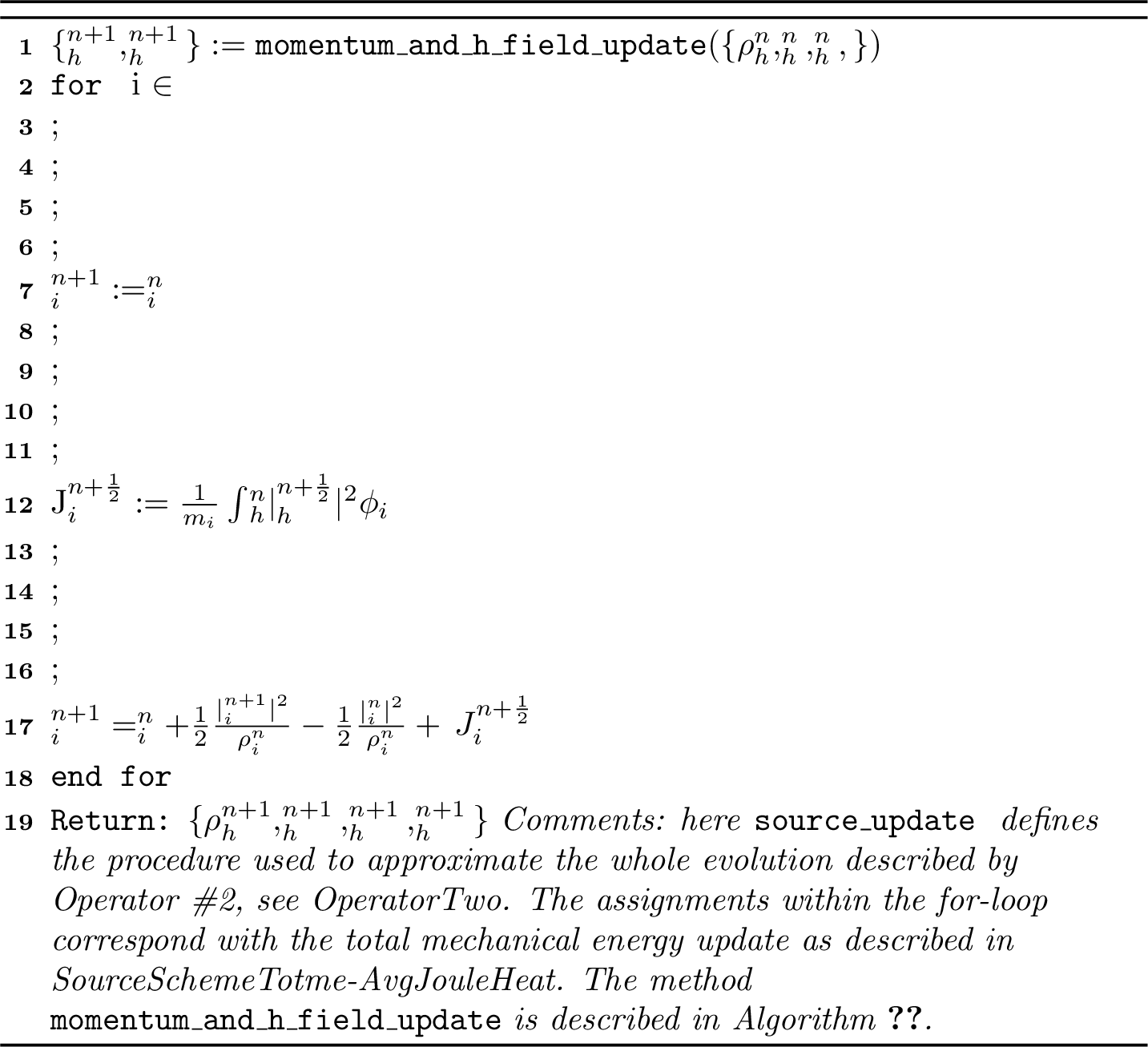
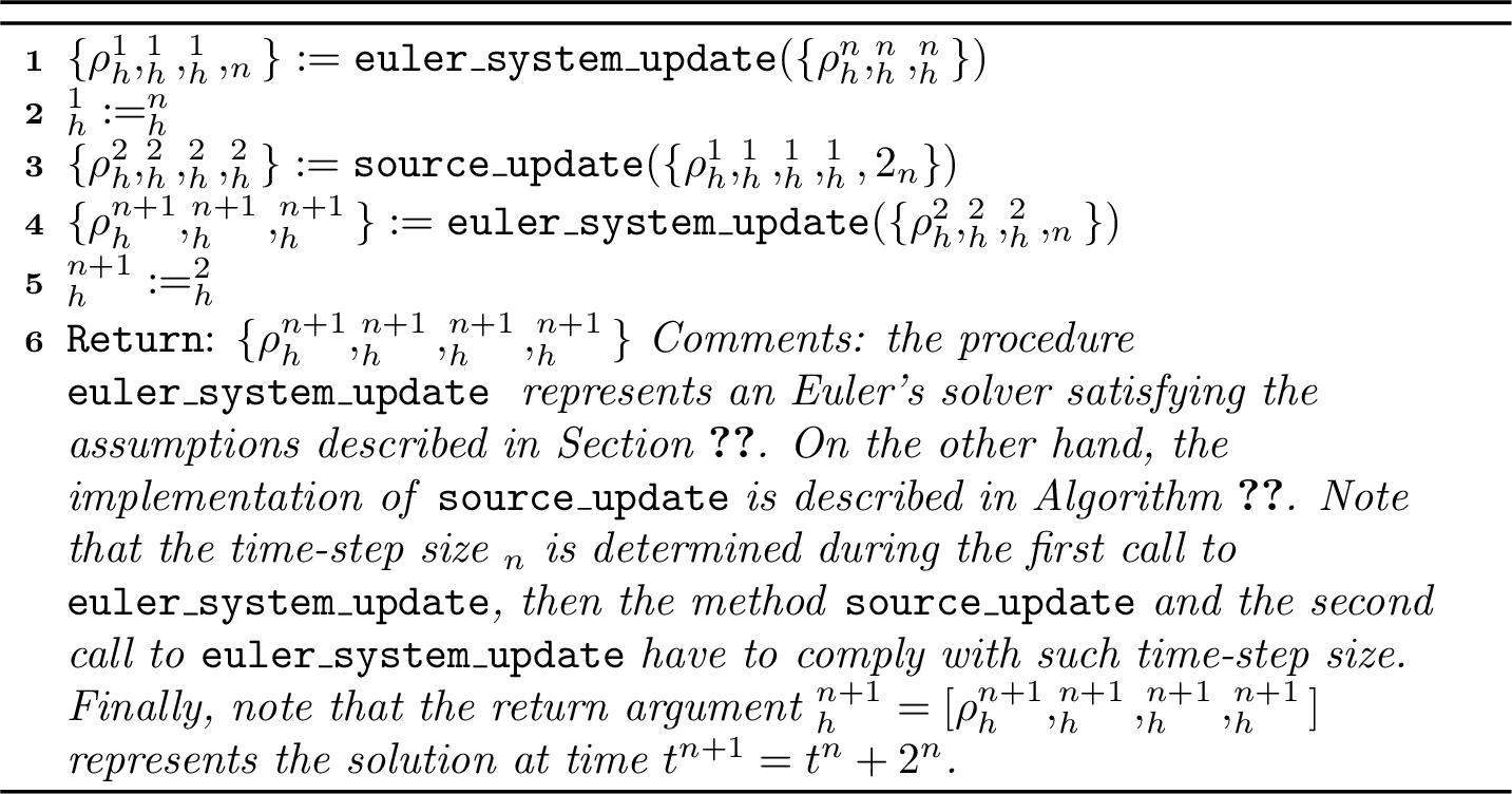
For the sake of completeness we summarize the properties satisfied by the method \(\texttt{hall\_mhd\_update}\) as defined in Algorithm 3 in the following proposition.
For the sake of simplicity that boundary conditions \(\mom\cdot\normal = 0\) and \(\Hfield \times \normal = \bzero\) are satisfied. Then
Energy stability. If we assume the method used to solve Euler’s equation
\(\texttt{euler\_system\_update}\) satisfies the conservation assumption ?? , then the output produced by method \(\texttt{hall\_mhd\_update}\) satisfies the total conservation of energy property \[\begin{gather} \sum_{i \in \HypVertices} m_i \totme_i^{n+1} + \tfrac{\mu}{2} \|\Hfield_h^{n+1}\|_{\Ltwo}^2 = \sum_{i \in \HypVertices} m_i \totme_i^{n} + \tfrac{\mu}{2} \|\Hfield_h^n\|_{\Ltwo}^2 . \end{gather}\]Admissibility. If the method used to solve \(\texttt{euler\_system\_update}\) satisfies the admissibility requirements outlined in the second bullet of Section 3.3, then the resulting solution \(\texttt{hall\_mhd\_update}\) is admissible as well. That is, \[\begin{align} \state_i^{n+1} = [\rho_i^{n+1}, \mom_i^{n+1}, \totme_i^{n+1}] \in \mathcal{A} \;\;\text{for all} \;i \in \HypVertices \end{align}\] where the set \(\mathcal{A}\) was defined in 41 .
Entropy-dissipation properties. If the method \(\texttt{euler\_system\_update}\) satisfies the entropy-dissipation inequality 42 then the method \(\texttt{hall\_mhd\_update}\) satisfies the entropy dissipation inequality as well. In particular we have that \[\begin{align} \sum_{i \in \HypVertices} m_i \eta(\state_i^{n+1}) \leq \sum_{i \in \HypVertices} m_i \eta(\state_i^{n}) \end{align}\]
Involution constraints. The method \(\texttt{hall\_mhd\_update}\) satisfies the following involution constraint: \[\begin{align} \label{InvolutionAgain} (\Hfield_h^{n+1}, \nabla \EpotTest_h)_{\Ltwo} = (\Hfield_h^{n}, \nabla \EpotTest_h)_{\Ltwo} \;\;\text{for all }\EpotTest_h \in\FESpacePotZero \end{align}\tag{50}\]
Proof. The proofs mostly boil down to invoking Proposition [Prop:sourceupdate], the assumptions on the hyperbolic solver described in Section 3.3, and the sequential nature of operator splitting:
Energy stability. It follows by a sequential argument: just use assumption ?? for the hyperbolic solver and and the discrete energy property ?? of Operator #2.
Admissibility. Again it follows by the sequential nature of operator splitting. Regarding Operator #1 we invoke the assumption in the third bullet of Section 3.3: the hyperbolic solver preserves admissibility. Regarding Operator #2 we invoke pointwise properties ?? which show that specific internal energy, temperature and specific entropy only increase during discrete evolution of Operator #2.
Entropy-dissipation. Let’s assume that the hyperbolic solver satisfies the entropy-dissipation property 42 . On the other hand, the the algorithm \(\texttt{source\_update}\) satisfies the inequality \(\eta(\state_i^{2}) \leq \eta(\state_i^{1})\), see expression ?? . Multiplying this inequality by \(m_i\) and adding for all \(i \in \HypVertices\) we obtain that the source-update scheme satisfies: \[\begin{align} \sum_{i \in \HypVertices} m_i \eta(\state_i^{2}) \leq \sum_{i \in \HypVertices} m_i \eta(\state_i^{1}) . \end{align}\] The global entropy-dissipation property follows by a sequential argument.
Involution constraints. We start by noting that the magnetic field \(\Hfield_h\) does not get modified during the evolution of Operator #1. On the other hand, \(\texttt{source\_update}\) preserves the involution property 50 as detailed in Proposition [Prop:sourceupdate] formula 38 . Therefore, it follows by the sequential nature of operator splitting that the method \(\texttt{hall\_mhd\_update}\) preserves the involution constraint.
◻
4 Numerical results↩︎
In this section, we demonstrate the validity and robustness of the proposed scheme. We first verify the solver by reproducing the whistler-wave dispersion relation and obtaining high-order convergence for the linearized equations (Section 4.1), before validating it in the nonlinear regime using the GEM challenge problem (Section 4.2). Finally, we present novel simulations of the Orszag–Tang vortex (Section 4.3) and conclude with a study of mesh sensitivity and the robustness of the proposed scheme (Section 4.4).
Throughout this section, we use \(P^1\) polynomials, ideal Equation of State with adiabatic constant \(\gamma=5/3\) and artificial resistivity constants \(c_{\text{low}} = 0.25\) and \(c_{\text{res}} = 1\). The CFL constant is taken 0.5 for all the simulations except for those in Section 4.3. The equations are expressed in nondimensional form, with velocities scaled by the Alfvén speed \(v_A=\HfieldComponent_0\sqrt{\mu/\rho_0}\), pressure by \(p_0=\mu\HfieldComponent_0^2\) and lengths scaled by the ion skin depth \(d_i\). Consequently, \(d_i\) denotes a non-dimensional parameter in this section.
4.1 Whistler wave↩︎
The simplest manifestation of the Hall term is the propagation of whistler waves. The linearized Hall resistive MHD equations admit theoretical wave solutions under uniform density and pressure, which can be used to perform an error convergence test. Similar tests have been carried out for the case of pure Hall MHD, see for example [27], [54]. Here, we also take resistivity into consideration.
More precisely, we choose a background field along the \(\unit_0\) direction and assume a small transverse wave perturbation propagating along \(\unit_0\): \[\begin{align} \Hfield = \HfieldComponent_0\,\unit_0 + \delta\Hfield,\qquad \delta\Hfield = \bigl(0,\,\delta \HfieldComponent,\,\delta \HfieldComponent\bigr)\,e^{i(kx_0 - \omega t)}. \end{align}\] Inserting this ansatz into the induction and momentum equations leads to the following dispersion relation for a right-hand polarized whistler wave \[\begin{align} \label{DispersionRelation} \omega = {\frac{\omega_H+\sqrt{\omega_H^2+4\omega_A^2}}{2}} - i\frac{r k^2}{2}\!\left(1 + \frac{\omega_H}{\sqrt{\omega_H^2+4\omega_A^2}}\right) + O(r^2), \end{align}\tag{51}\] with \(\omega_H := d_ik^2\HfieldComponent_0/\rho\) and \(\omega_A^2:=k^2\HfieldComponent^2_0/\rho\). The corresponding wave solution is \[\begin{align} \label{whislerSolution} \begin{aligned} v_{1} &= -\delta v \;e^{\Im (\omega)t}\cos(kx_0 - \Re(\omega) t), & \HfieldComponent_{1} &= \;\;\delta \HfieldComponent \;e^{\Im (\omega)t}\cos(kx_0 - \Re(\omega) t), \\ v_{2} &= \;\;\delta v \;e^{\Im (\omega)t}\sin(kx_0 - \Re(\omega) t), & \HfieldComponent_{2} &= -\delta \HfieldComponent \;e^{\Im (\omega)t}\sin(kx_0 - \Re(\omega) t), \end{aligned} \end{align}\tag{52}\] where \(\delta v\) is related to \(\delta \HfieldComponent\) through the momentum equation as \[\begin{align} \displaystyle\delta v = \frac{\,k \HfieldComponent_0}{\omega\rho}\,\delta \HfieldComponent. \end{align}\] We follow a setup analogous to that of [55], with a doubly periodic domain \([-L_x, L_x]\times[-L_y, L_y]\) with \(L_x=80/3\) and \(L_y=20\) with a propagation direction \(\unit_0\) forming an angle \(\varphi=\arctan(4/3)\) with respect to the \(x\)-axis. In the computational frame, the initial perturbation phase becomes \({\Phi(x,y) = k(x\cos\varphi + y\sin\varphi).}\) This results in the following set of initial conditions \[\begin{align} v_{x} &= \;\;\delta v \sin\varphi\cos\Phi, & \HfieldComponent_{x} &= \HfieldComponent_0\cos\varphi - \delta \HfieldComponent \sin\varphi\cos\Phi, & \rho &=\rho_0,\\ v_{y} &= -\delta v \cos\varphi\cos\Phi, & \HfieldComponent_{y} &= \HfieldComponent_0 \sin\varphi +\delta \HfieldComponent \cos\varphi\cos\Phi, & p &=p_0,\\ v_{z} &= \;\;\delta v \sin\Phi, & \HfieldComponent_{z} &= -\delta \HfieldComponent \sin\Phi. \end{align}\] We set \(\rho_0=1\), \(\HfieldComponent_0=0.2\), \(p_0=5.12\times 10^{-4}\), \(d_i = 1\), \(\resist = 0.001\) and \(\lambda = 2\pi/k = 32\). The initial perturbation \(\delta \HfieldComponent= 0.0001\) is taken small enough such that nonlinear effects of the PDE are negligible. The relative \(L^2\) norm error is computed between the numerical solution and the theoretical solution 52 after a full period \(T = 2\pi/\Re(\omega)\).
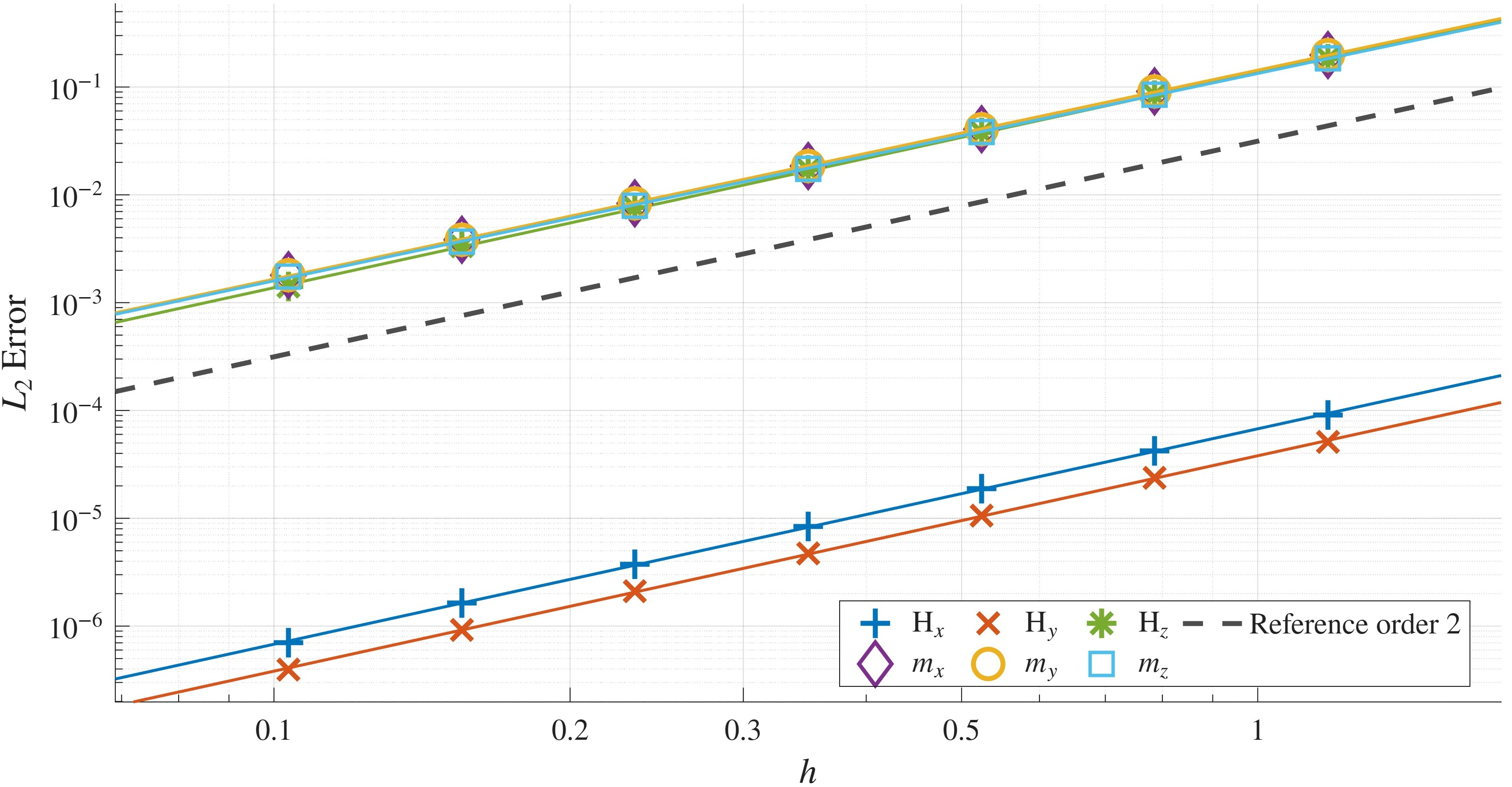
The convergence results over several mesh sizes are collected in Table 1 and plotted in Figure 4 along reference rate 2 lines, corresponding to the expected convergence for \(P_1\) polynomials. The rates are computed using least squares. The method achieves near-optimal convergence rates for all the components, successfully capturing the characteristic dispersion relation for whistler waves.
| \(L^2\) error in \(\Hfield\) | \(L^2\) error in \(\mom\) | |||||
| Mesh | \(\HfieldComponent_x\) | \(\HfieldComponent_y\) | \(\HfieldComponent_z\) | \(\momComponent_x\) | \(\momComponent_y\) | \(\momComponent_z\) |
| \(64 \times 48\) | 9.10E-05 | 5.12E-05 | 1.83E-01 | 1.97E-01 | 1.97E-01 | 1.84E-01 |
| \(96 \times 72\) | 4.21E-05 | 2.37E-05 | 8.44E-02 | 9.13E-02 | 9.13E-02 | 8.52E-02 |
| \(144 \times 108\) | 1.87E-05 | 1.05E-05 | 3.78E-02 | 4.08E-02 | 4.08E-02 | 3.83E-02 |
| \(216 \times 162\) | 8.44E-06 | 4.75E-06 | 1.71E-02 | 1.85E-02 | 1.85E-02 | 1.75E-02 |
| \(324 \times 243\) | 3.74E-06 | 2.10E-06 | 7.59E-03 | 8.35E-03 | 8.35E-03 | 7.95E-03 |
| \(486 \times 364\) | 1.65E-06 | 9.26E-07 | 3.33E-03 | 3.84E-03 | 3.84E-03 | 3.67E-03 |
| \(729 \times 546\) | 7.04E-07 | 3.96E-07 | 1.41E-03 | 1.81E-03 | 1.81E-03 | 1.74E-03 |
| Rates | 1.998 | 1.998 | 1.995 | 1.938 | 1.938 | 1.923 |
4.2 GEM magnetic reconnection challenge↩︎
For a nonlinear verification of the scheme, we consider the Geospace Environmental Modeling (GEM) magnetic reconnection challenge. First introduced by [9], it is markedly the standard and most well-studied test for Hall MHD, as it is designed to reproduce magnetic reconnection on a perturbed Harris sheet, where the Hall contribution is known to be critical to obtain fast reconnection rates. Although no exact solution is known for this problem, extensive numerical research has been carried out, and the reconnection rates produced can be compared quantitatively.
We consider a rectangular domain \([0, L_x]\times[0, L_y]\) with \(L_x=25.6\) and \(L_y=12.8\) with periodic boundary conditions for the \(x\)-axis. For the \(y\)-axis, we use homogeneous natural boundary conditions6 by dropping the boundary terms arising from integration by parts in the weak formulation, see expression 32 . The resistivity and ion-skin depth are taken to be \(r=0.005\) and \(d_i=1\), respectively. We use the following set of initial conditions: \[\begin{align} \rho &= \rho_0\sech^2\!\left(\frac{y-y_0}{\lambda}\right)+\rho_\infty, \quad \quad p = p_0 - \frac{{\HfieldComponent}_0^2}{2}\tanh^2\!\left(\frac{y-y_0}{\lambda}\right), \quad \quad \vel = \bzero, \\ {\HfieldComponent_x} &= {\HfieldComponent}_0\tanh\!\left(\frac{y-y_0}{\lambda}\right) + \frac{\psi_0}{L_y}\pi\cos\!\left(\frac{2\pi x}{L_x}\right)\sin\!\left(\frac{\pi(y-y_0)}{L_y}\right), \\ {\HfieldComponent_y} &= -\frac{\psi_0}{L_x}2\pi\sin\!\left(\frac{2\pi x}{L_x}\right)\cos\!\left(\frac{\pi(y-y_0)}{L_y}\right), \\ {\HfieldComponent_z} &= 0, \end{align}\] where \(\rho_0 = 1\), \(\rho_\infty = 0.2\), \({\HfieldComponent}_0 = 1\), \(p_0 = 0.6\), \(\lambda = 0.5\), \(y_0=6.4\) and \(\psi_0 = 0.1\). Four snapshots are illustrated in Figure 5 for the out-of-plane current density \(J_z=(\curl{}\Hfield)_z\) using a mesh of 1024\(\times\)1024 elements. Starting from the perturbed Harris equilibrium, the current sheet thins around the center of the domain until it collapses into an X-line. The reconnection rate begins to increase at \(t\approx18.5\) [panel (a)], marking the onset of fast, Hall-mediated reconnection. The precise location of the onset time is particularly sensitive to space and time discretization. This is notable for the cases of coarse meshes that do not fully resolve high-frequency whistler waves, and for the case of anisotropic meshes where the onset can be delayed. After the onset, magnetic energy is rapidly converted into kinetic and thermal energy, driving an outflow jet away from the X-line [panel (b)]. Once the jet reaches the periodic boundary, it thickens and interacts with itself, and the current density at the center reverses sign [panels (c)–(d)].
The reconnected flux, \(\Psi(t) = \int_{L_x/2}^{L_x}\HfieldComponent_y(x, y=L_x/2)\;dx\) is plotted in Figure 6 for both Hall-resistive MHD and only resistive MHD. The rate of reconnection is considerably larger for the Hall simulation, agreeing with the results in, for instance, [9], [25], [27].
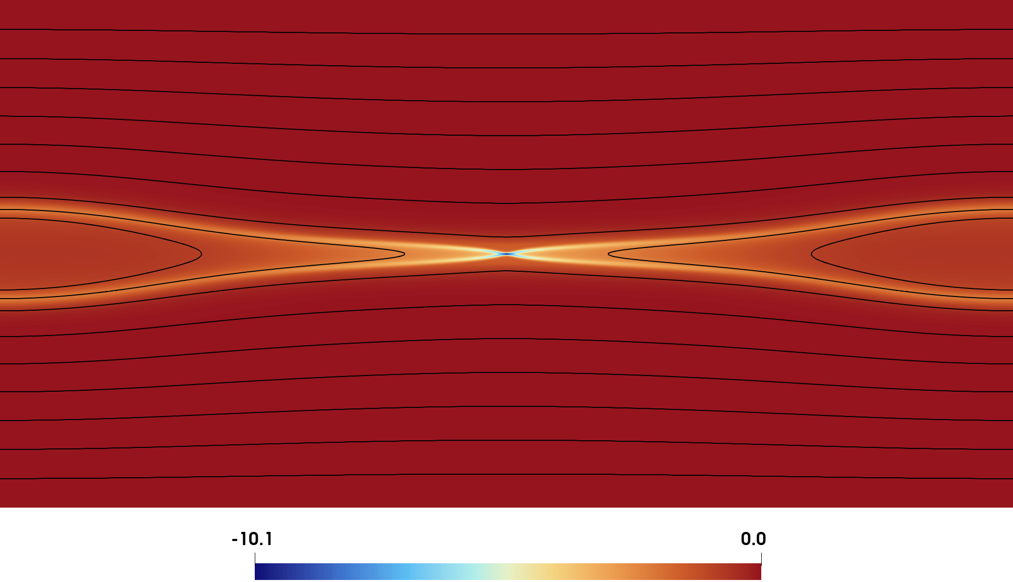
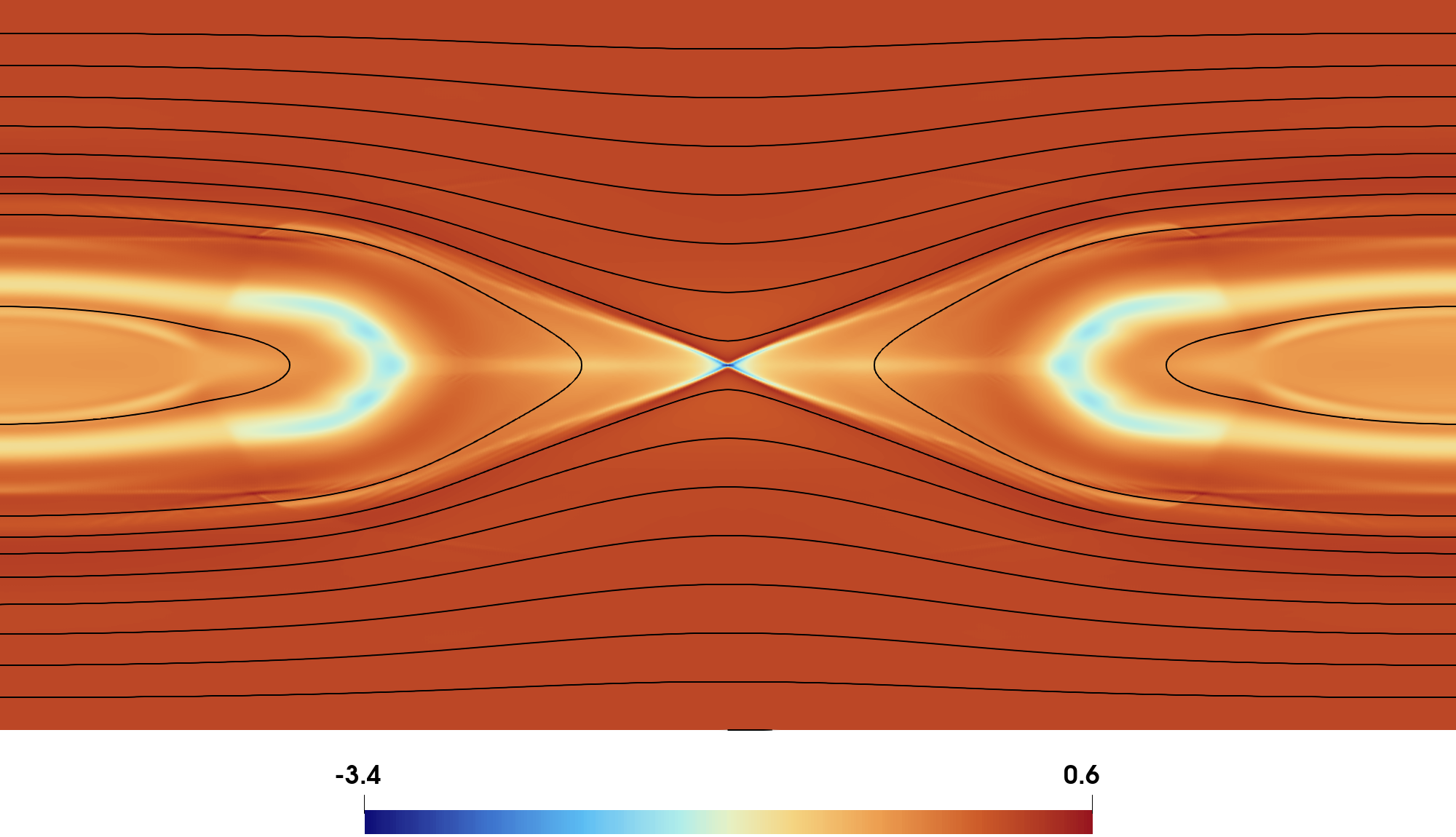
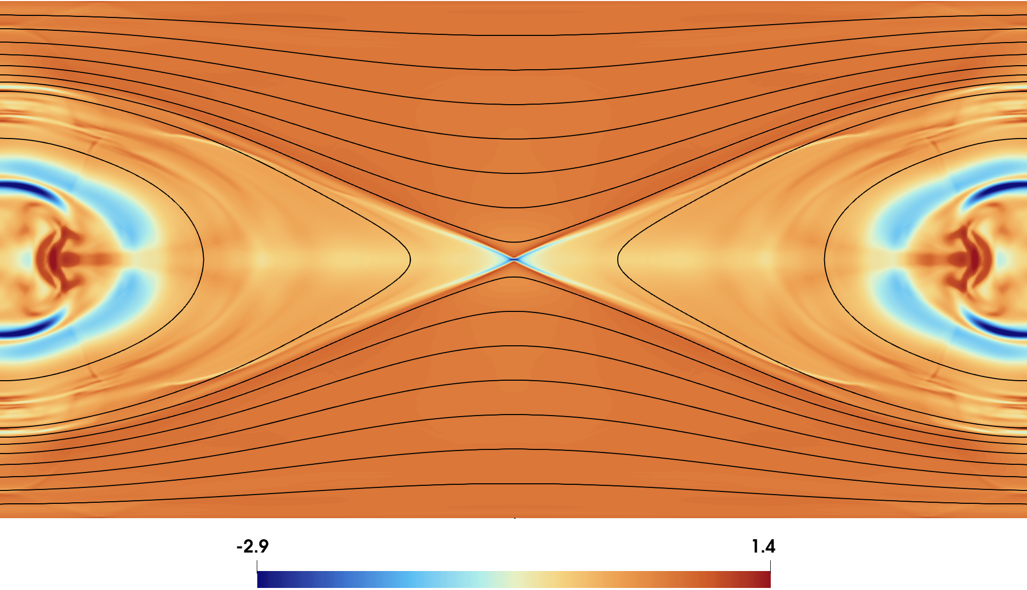
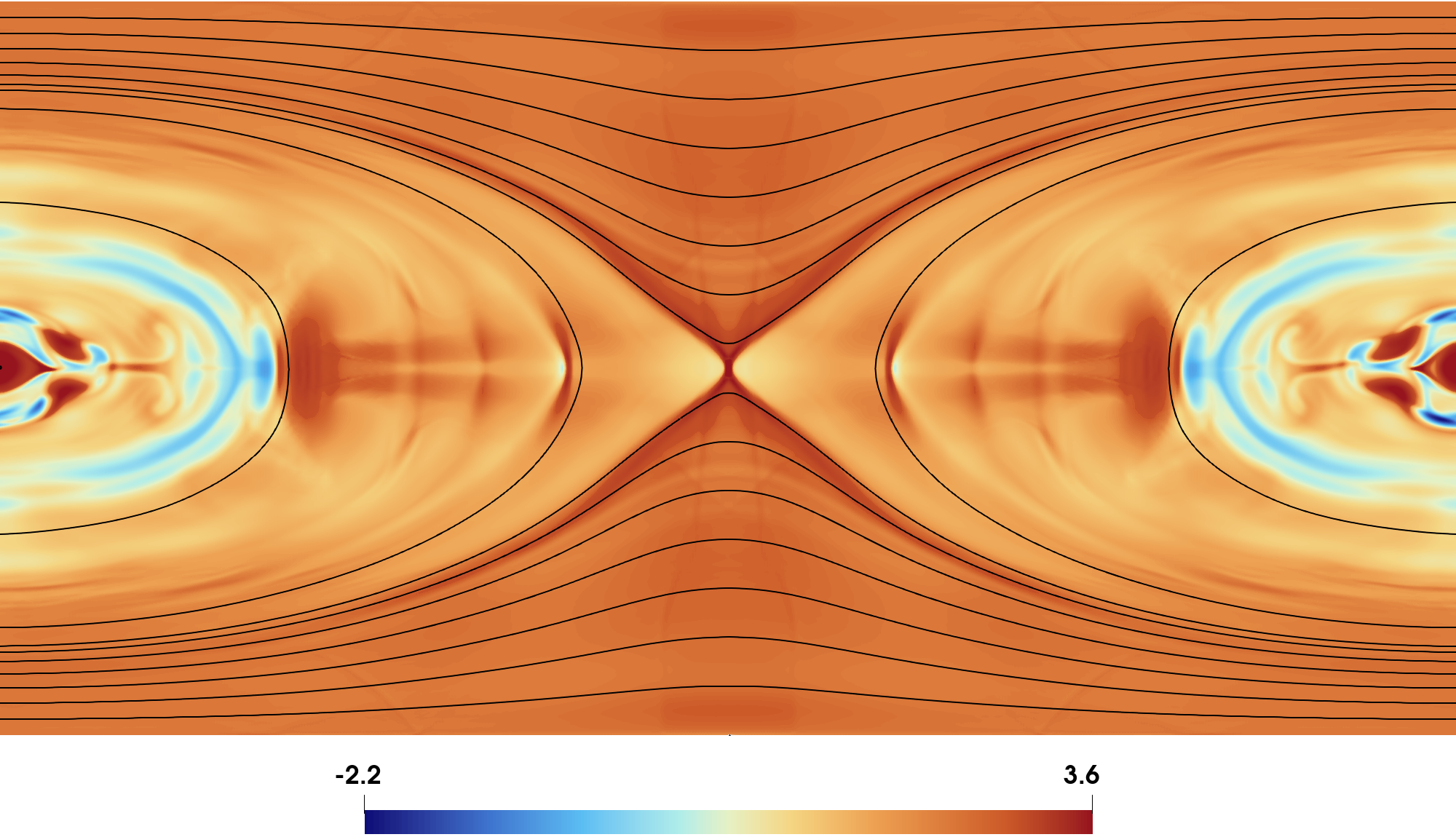
Figure 5: GEM magnetic reconnection challenge out-of-plane component of the current density for \(1024\times1024\) elements at times \(t=18\), \(25\), \(30\), and \(40\). Contour plots of the magnetic field \(\Hfield\) are shown in black.. a — \(t=18.5\), b — \(t=25\), c — \(t=30\), d — \(t=40\)

4.3 Orszag–Tang vortex↩︎
The Orszag–Tang vortex is a standard benchmark for ideal MHD [56], as it evaluates the capability of a numerical scheme to resolve nonlinear shocks and turbulence behavior. The Orszag–Tang vortex has rarely been considered in the context of Hall MHD. While there exist studies adopting a quasi-incompressible formulation [57]–[59], investigations in the compressible regime remain limited. Bard et al. [54] simulated the compressible Hall MHD Orszag–Tang problem, but without explicit resistivity, therefore lacking a mechanism to trigger reconnection. Multi-component kinetic frameworks [60] have been shown to recover the compressible Hall-resistive structures asymptotically in the fluid limit. However, to the best of our knowledge, this work presents the first macroscopic simulation of the fully compressible, resistive Hall-MHD equations for the Orszag–Tang vortex, systematically evaluating the flow across a wide range of non-dimensional ion skin depth values, from purely resistive MHD to strongly Hall-dominated regimes, up to \(t=1\).
The setup for the Orszag–Tang vortex test consists of a periodic square domain \(\Omega = [0,1]\times[0,1]\) with initial data \[\begin{align} (\rho, \vel, p, \Hfield) = \left( \frac{25}{36\pi}, (-\sin(2\pi y), \sin(2\pi x), 0), \frac{5}{12\pi}, \left( -\frac{\sin(2\pi y)}{\sqrt{4\pi}}, \frac{\sin(4\pi x)}{\sqrt{4\pi}},0 \right) \right), \end{align}\] We choose a resistivity \(\resist = 0.001\), sufficiently small for resistive diffusion to remain subdominant compared to the Hall term. Previous studies have shown that the reconnection rate is largely insensitive to the particular mechanism responsible for breaking the frozen-in condition [9], and the values of \(d_i\) employed here are sufficient for the Hall effects to trigger reconnection, as discussed later. Although \(\resist = 0.005\) is commonly used in the GEM setup and already produces reconnection, we have (intentionally) adopted a smaller value in order to assess the robustness of the solver under more demanding conditions.
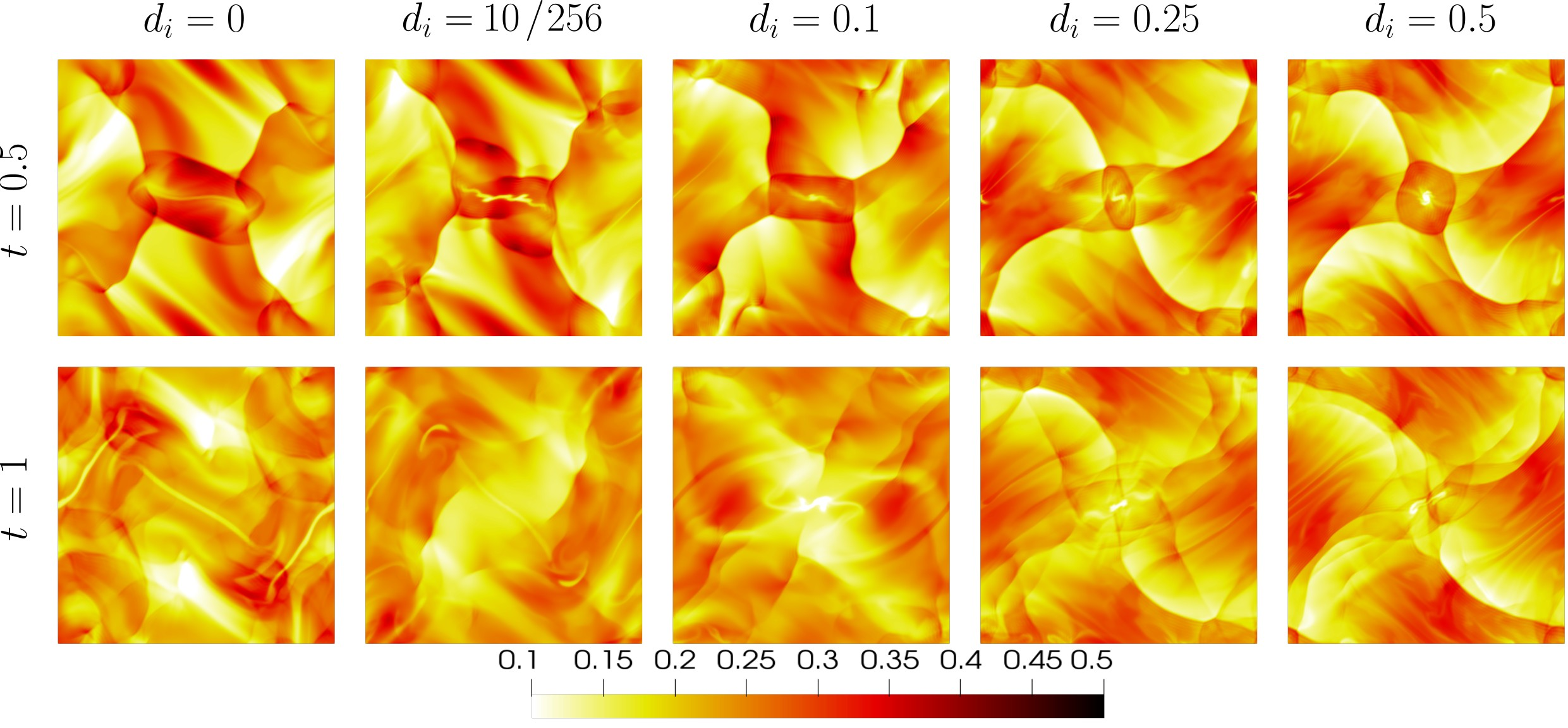
The density fields at \(t=0.5\) and \(t=1\) are displayed in Figure 7 for a \(256\times256\) nodes grid, and several values of the ion skin depth. We include \(d_i=0\) as a purely resistive reference case, \(d_i=256/10\) such that the characteristic Hall scale is resolved by approximately 10 grid points, and \(d_i=0.1,\:0.25,\:0.5\) to illustrate a strongly Hall-dominated regime. We stress that these \(d_i\) values are relatively large and make the problem numerically demanding. For instance, when \(d_i=0.5\), the Hall term operates on a length scale comparable to half the domain size, much larger than in typical benchmark configurations. Under these conditions, the electron velocity is between one and two orders of magnitude greater than the ion velocity. The Jacobian becomes less coercive, which can impose very restrictive time-step constraints; see 7 for details. For \(d_i=0.25\) and 0.5, the CFL constant was lowered to 0.1.
The results shown in Figure 7 reveal that in the purely resistive case [first column], the solution resembles a more diffusive version of the ideal case, as magnetic reconnection occurs at a significantly slower rate compared to Hall simulations. When increasing the strength of \(d_i\) and consequently the scale of Hall dynamics, the solution is affected rather drastically. A low-density core forms at the center of the domain, and a different shock distribution emerges.
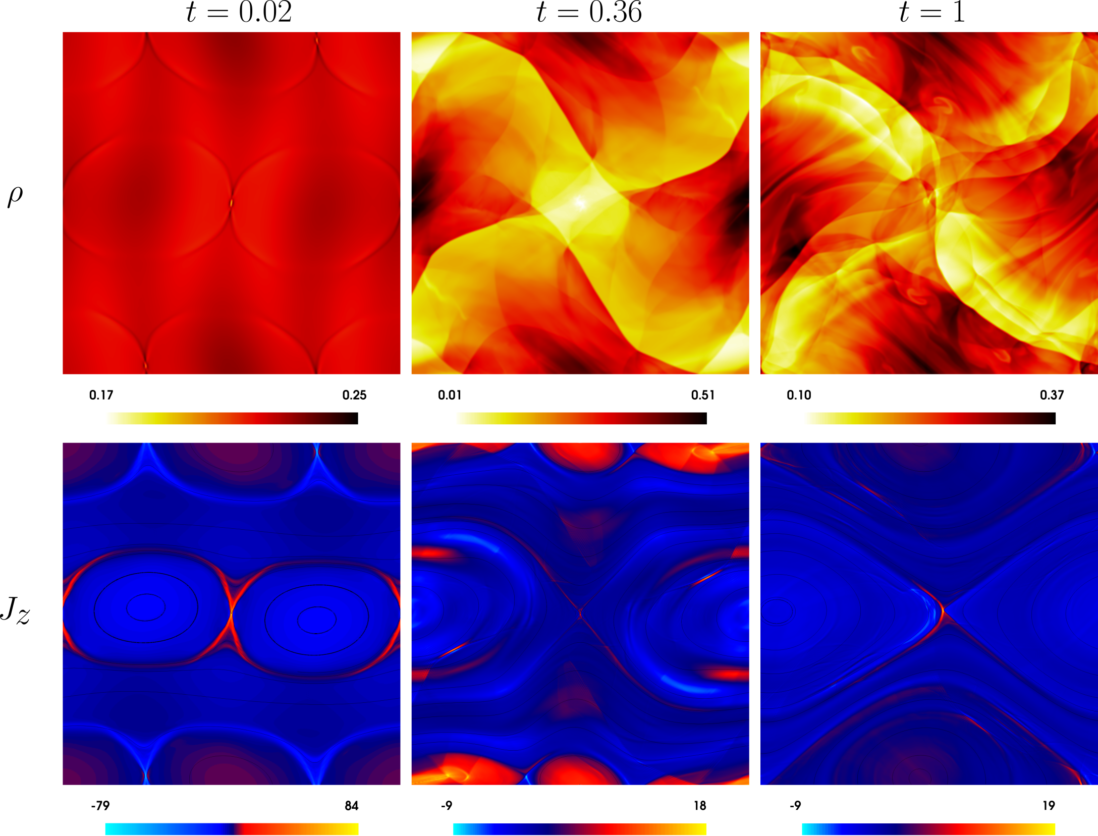
To better illustrate the solution in the so-called magnetically dominated regime, Figure 8 shows a fine-mesh computation with \(724\times724\) elements of the density and out-of-plane current distributions for the highest value of the ion skin depth tested, \(d_i=0.5\). A CFL of \(0.05\) was required to guarantee coercivity of the Jacobian. Under these conditions, magnetic reconnection develops almost immediately: at \(t=0.02\) an X-point geometry has already formed and the current density reaches its maximum value of the simulation, with \(|J_z|\sim 84\). As reconnection proceeds, the magnetic energy is converted into kinetic and thermal energy, producing a low-density core and a GEM-like outflow jet structure emanating from the central reconnection site, as seen in \(t=0.36\). Finally, by \(t=1\) the flow has transitioned into a fully turbulent state: the density field shows a rich collection of fine-scale filaments and shear layers. The peak current density remains comparable to that at earlier times, and its evolution stabilizes. Overall, the evolution of the magnetic topology is qualitatively consistent with the reconnection geometries reported by Liu and Xu [60].
4.4 Mesh behaviour study↩︎
Magnetic reconnection is a process that involves large, localized gradients and steep hyperbolic fronts in reduced regions of the computational domain. In addition, the Hall term introduces a highly asymmetric and nonlinear contribution to the dynamics. For that reason, we assess the sensitivity of the numerical scheme with respect to mesh-imprint artefacts by executing the GEM magnetic reconnection challenge across four distinct mesh configurations with a comparable number of degrees of freedom:
Criss-cross structured mesh. Completely symmetric. The mesh consists of 256\(\times\)256 rectangular cells, each divided into two elements in an alternating, symmetrical fashion, giving a total of 65,792 DOF for the scalar finite element space \(\FESpaceHypComp\).
Directionally-biased structured mesh. Also built from 256\(\times\)256 rectangular cells, each subdivided into two triangular elements, with all diagonals oriented to the right.
Isotropic unstructured mesh. Generated with a Frontal-Delaunay algorithm, yielding nearly equilateral triangles throughout the domain. The number of degrees of freedom is 65,444 DOF for the scalar finite element space \(\FESpaceHypComp\).
Anisotropic unstructured mesh. Generated with a Delaunay algorithm under an anisotropic sizing field, so that triangles are stretched to approximately 0.1 wide by 0.05 tall, matching the 2:1 aspect ratio used in the structured meshes. This resulted in 72,918 DOF for the scalar finite element space \(\FESpaceHypComp\).
The 2:1 aspect ratio is chosen deliberately: the diffusion layer that develops along the \(y\)-axis requires finer resolution in that direction to capture accurate reconnection rates, so meshes #1, #2, and #4 all preserve this anisotropy while mesh #3, which is isotropic, does not.
Figure 9 shows a snapshot of GEM at \(t=35\) for the four described meshes. Qualitatively, differences can be observed for each mesh. The directionally-biased mesh #2 breaks the symmetry of the reconnected structures, mirroring the orientation of the mesh diagonals. The anisotropic unstructured mesh #4 struggles to form a single, well-defined X-line: the current sheet appears more elongated, and two X-points form symmetrically about the domain center before eventually merging, after which the reconnection region settles with a slight offset from the center. We also note that the reconnected region is (somewhat) more singular in mesh #1 than meshes #2, #3 and #4. The singular nature of this solution caught our attention in our early attempts at computing this solution without artificial viscosity, requiring a significant number of Newton iterations.
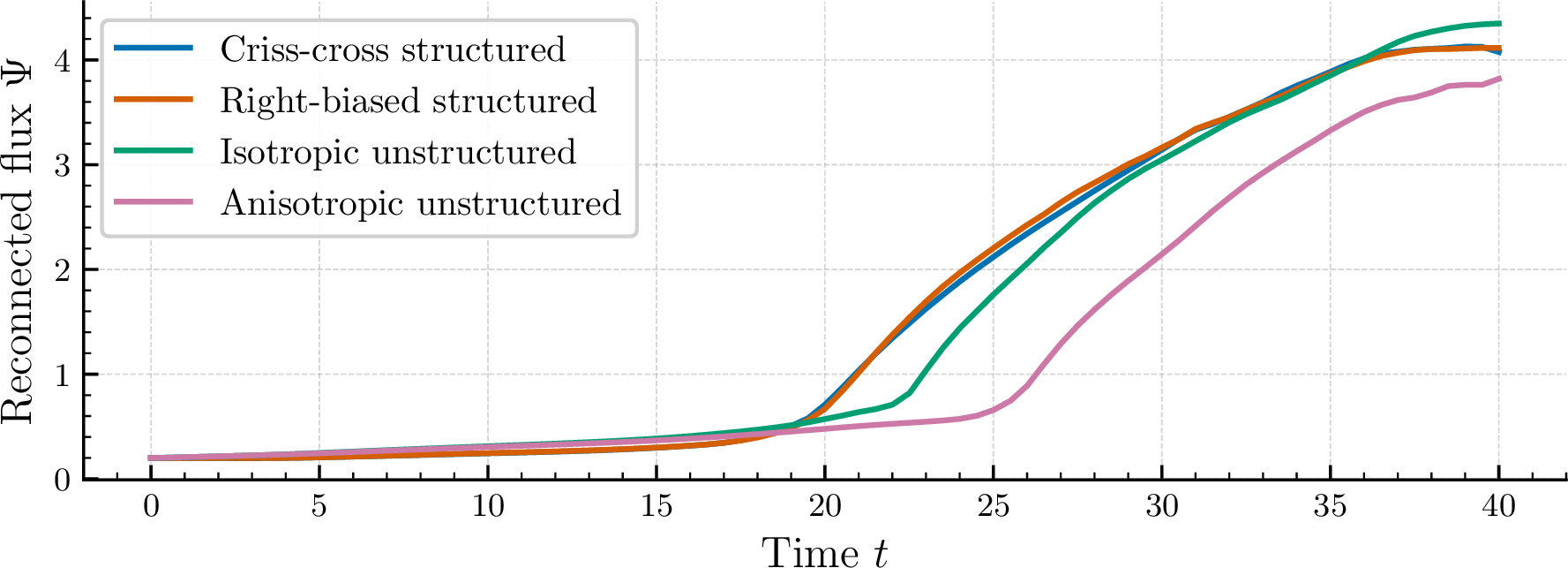
The reconnected flux for each mesh is shown in Figure 10. Despite the differences noted above, all four meshes eventually produce comparable reconnection rates. The main sensitivity is found in the onset of fast reconnection. Mesh #4 shows the most pronounced delay, consistent with the transient double-X-point behavior: the merging of the two X-points postpones the onset of fast reconnection relative to meshes #1 and #2. Mesh #3 shows a smaller, secondary delay, which we attribute to its isotropic triangles under-resolving the diffusion layer relative to the anisotropic meshes, despite having a comparable overall number of degrees of freedom.
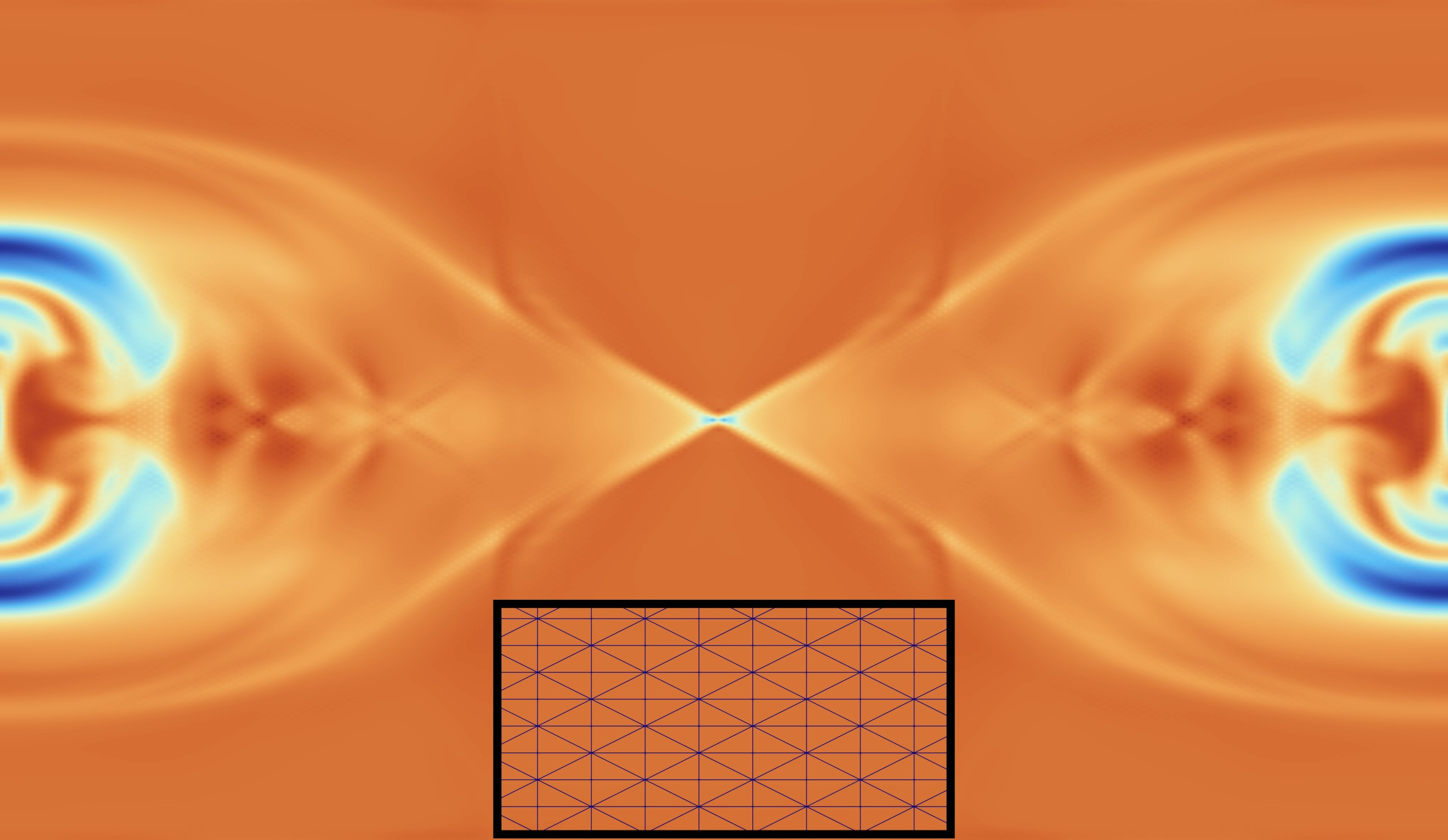
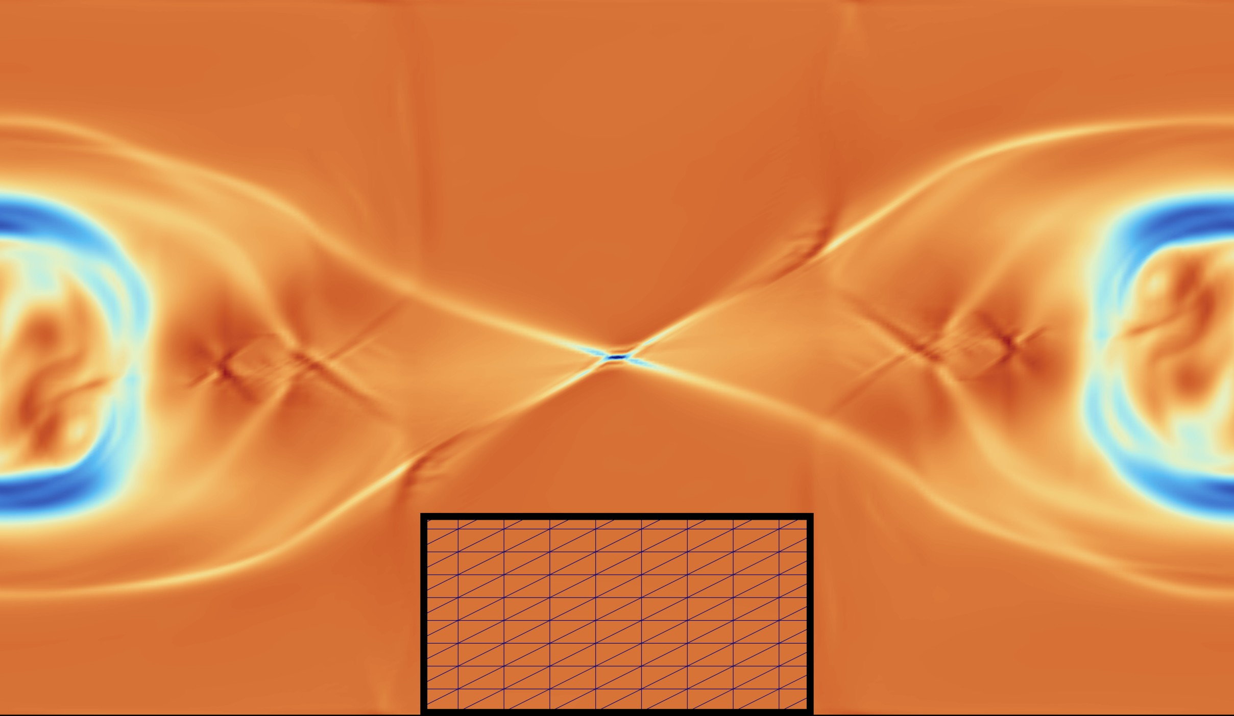
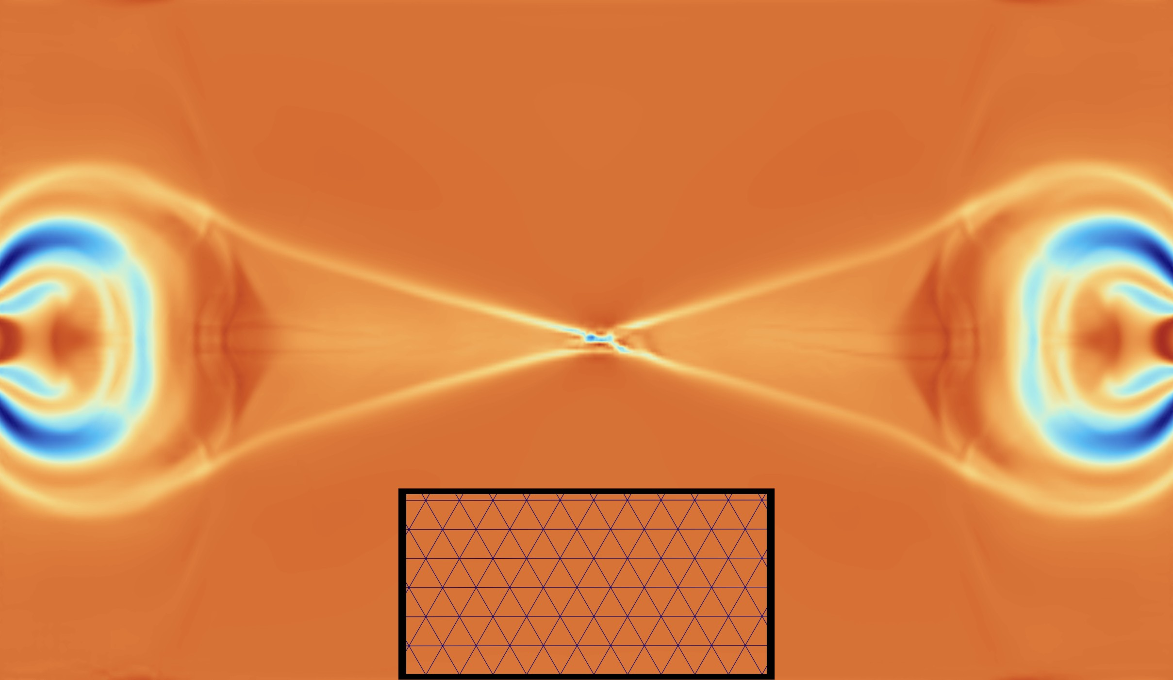
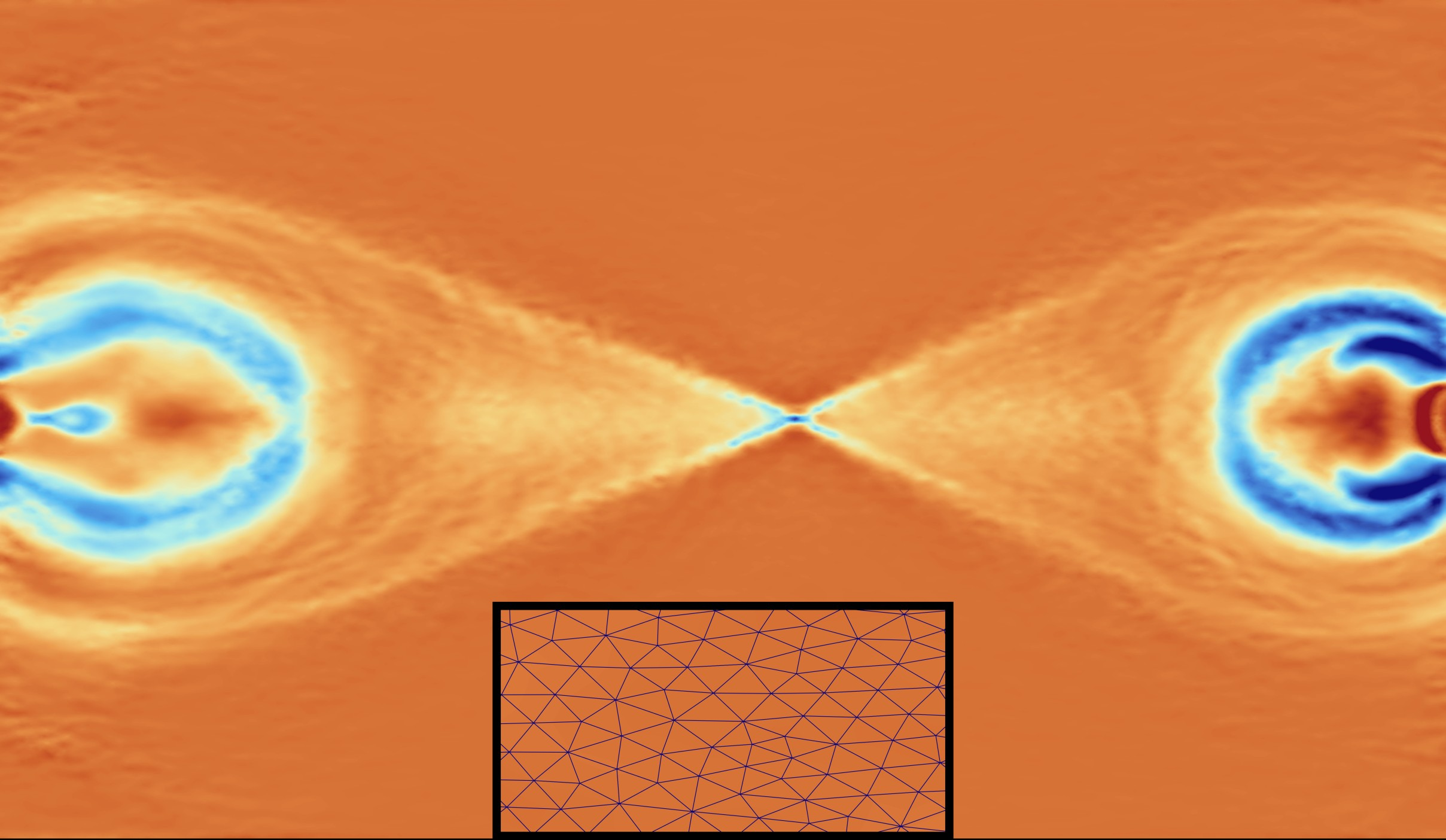
Figure 9: Comparison of the GEM magnetic reconnection challenge for three mesh topologies at \(t=35\). The number of degrees of freedom used for (a) and (b) is 65,792, while 65,444 for (c) and 72,918 for (d).. a — Criss-cross structured mesh, b — Directionally-biased structured mesh, c — Isotropic unstructured mesh, d — Anisotropic unstructured mesh
5 Acknowledgments↩︎
IT wants to acknowledge the continuous support of NSF grant DMS-2409841; Sandia National Laboratories LDRD contract agreement #1964744, award number #2644205; and Simons Foundation Travel Award for Mathematicians. MN and RV are supported by the Swedish Research Council (VR) under grant numbers 2021-04620.
6 Thermodynamics and equations of state↩︎
A thermal Equation of State7 is a 2-dimensional manifold embedded in \(\mathbb{R}^3\). More precisely, such a manifold is given by the set of points [61], [62]: \[\begin{align} \label{EOSmanifold} (\specv, e, s(\specv, e)) \subset \mathbb{R}^3 \end{align}\tag{53}\] where \(\specv = \tfrac{1}{\rho}\) is the specific volume, \(e = \tfrac{\totme}{\rho} - \frac{1}{2} |\vel|^2\) is the specific internal energy, and \(s(\specv, e):\mathbb{R}^+ \times \mathbb{R}^+ \rightarrow \mathbb{R}\) is the specific entropy. From expression 53 it is tacitly understood that \(\specv\) and \(e\) are the independent variables while \(s\) is the dependent variable. For any practical purpose, we may say that the specific entropy \(s(\specv, e)\) is the EOS, since it is all you need to describe the manifold 53 . For instance, for the case of the Nobel-Abel-Stiffened-Gas, the specific entropy is given by [63]: \[\begin{align} s(\rho, \specinte) &= c_v \ln \Big( (\gamma - 1) \frac{\rho(e - q) + p_{\infty} (\rho b - 1)}{1 - \rho b} \Big) - c_v \gamma \ln \Big(\frac{(\gamma - 1) c_v \rho}{1 - \rho b} \Big) + s_0. \end{align}\] where \(c_v > 0\), \(0 \leq b < +\infty\), \(q > 0\), \(p_{\infty} \in \mathbb{R}\), and \(1 < \gamma \leq \tfrac{5}{3}\). For the very specific case of \(b = 0\), \(q = 0\) and \(p_{\infty} = 0\), the NASG EOS becomes the well-known ideal gas specific entropy. In broad terms, an EOS describes all thermodynamically accessible states of the substance or fluid: i.e. not every triple of points \((\specv,e,s) \in \mathbb{R}^+ \times \mathbb{R}^+ \times \mathbb{R}\) represents an accessible thermodynamical state.
The pressure formula is a direct consequence of the Gibbs identity (an exact differential, see [61]). More precisely, we have that the Gibbs identity is given by: \[\begin{align} \mathrm{d}s = \frac{1}{\temp}\mathrm{d}e + \frac{p}{\temp} \mathrm{d}\specv \;\;\text{where} \;\;s = s(\specv, e) \, , \; \end{align}\] which immediately implies that: \[\begin{align} \label{PressureEpist} \frac{\partial s}{\partial e} = \frac{1}{\theta} \;\;\text{and} \;\; \frac{\partial s}{\partial v} = \frac{p}{\temp} \;\;\text{therefore} \;\; p = p(\specv, e) = - \rho^2 \frac{\partial s}{\partial \rho} \Big[\frac{\partial s}{\partial e}\Big]^{-1}. \end{align}\tag{54}\] In this paper we assume that the pressure is computed from its corresponding specific entropy as described in 54 . The precise formula of the specific entropy \(s(\specv, e)\) should be compatible with basic thermodynamic constraints. We will make use of the following standard assumptions:
Positivity of the temperature. We assume that: \[\begin{align} \label{posTempAssump} \frac{\partial s}{\partial e} = \frac{1}{\theta} > 0 \;\;\text{for every} \;\; (\specv, e) \in \mathbb{R}^+ \times \mathbb{R}^+ \;\;\text{in the domain of} \;s(\specv,e) \end{align}\tag{55}\] Note, that in general, the domain of the specific entropy \(s(\specv, e)\) maybe a strict subset of the positive quadrant \(\mathbb{R}^+ \times \mathbb{R}^+\), see [50] for more details.
Thermodynamic stability. We assume that the specific entropy is concave with respect to \(\specv\) and \(e\). More precisely, we have that the following properties should hold [61], [62]: \[\begin{align} \label{convexAssump} \frac{\partial^2 s}{\partial^2 v} \leq 0 \;, \;\; \frac{\partial^2 s}{\partial^2 e} \leq 0 \;\;\text{and} \;\; \frac{\partial^2 s}{\partial^2 v} \frac{\partial^2 s}{\partial^2 e} - \Big(\frac{\partial^2 s}{\partial v \partial e}\Big)^2 \geq 0 \end{align}\tag{56}\] The condition \(\tfrac{\partial^2 s}{\partial^2 e} \leq 0\) is particularly relevant in this paper, since it implies that the monotonicity condition: \[\begin{align} \label{tempMono} \frac{\partial }{\partial e}\theta(\specv,e) \geq 0 \end{align}\tag{57}\] holds true. Monotonicity condition 57 implies that our equation of state is such that an increase in specific internal energy, at constant density, can only produce a non-negative increment of temperature.
7 Jacobian of the Newton Iteration and its properties↩︎
We may rewrite the scheme 33 as: find \(\{\vel_h^{n+1}, \Hfield_h^{n+1}\} \in \FESpaceHypComp^d \times \FESpaceHtangent\) satisfying \[\begin{align} \label{SolutionNewton00} a([\vel_h^{n+1}, \Hfield_h^{n+1}], [\veltest_h, \Htest_h]) = f([\vel_h^{n}, \Hfield_h^{n}], [\veltest_h, \Htest_h]) \;\;\text{for all} \;\; [\veltest_h, \Htest_h] \in \FESpaceHypComp^d \times \FESpaceHtangent \end{align}\tag{58}\] where \(a([\vel_h^{n+1}, \Hfield_h^{n+1}], [\veltest_h, \Htest_h])\) is a nonlinear map defined by: \[\begin{align} &a([\vel_h^{n+1}, \Hfield_h^{n+1}], [\veltest_h, \Htest_h]) := \langle \rho_h^n \vel_h^{n+1} , \veltest_h \rangle + \mu (\Hfield_h^{n+1}, \Htest_h)_{\Ltwo} \\ &- \tfrac{1}{4} \dt \mu ( \curl{}\Hfield_h^{n+1} \times \Hfield_h^{n}, \veltest_h )_{\Ltwo} - \tfrac{1}{4} \dt \mu (\curl{}\Hfield_h^{n+1} \times \Hfield_h^{n+1}, \veltest_h )_{\Ltwo} \\ &- \tfrac{1}{4} \dt \mu (\curl{}\Hfield_h^{n} \times \Hfield_h^{n+1}, \veltest_h )_{\Ltwo} + \tfrac{1}{4} \dt \mu (\curl{}\Htest_h \times \Hfield_h^{n} , \vel_h^{n+1} )_{\Ltwo} \\ &+ \tfrac{1}{4} \dt \mu (\curl{}\Htest_h \times \Hfield_h^{n+1} , \vel_h^{n} )_{\Ltwo} + \tfrac{1}{4} \dt \mu (\curl{}\Htest_h \times \Hfield_h^{n+1} , \vel_h^{n+1} )_{\Ltwo} \\ &+ \tfrac{1}{2} \dt (\resist_h \curl{}\Hfield_h^{n+1},\curl{}\Htest_h)_{\Ltwo} + \tfrac{1}{4} \mu d_i \dt \big(\tfrac{1}{\rho_h^n} \curl{}\Hfield_h^{n} \times \Hfield_h^{n+1}, \curl {}\Htest_h \big)_{\Ltwo} \\ &+ \tfrac{1}{4} \mu d_i \dt \big(\tfrac{1}{\rho_h^n} \curl{}\Hfield_h^{n+1} \times \Hfield_h^{n}, \curl {}\Htest_h \big)_{\Ltwo} \\ &+ \tfrac{1}{4} \mu d_i \dt \big(\tfrac{1}{\rho_h^n} \curl{}\Hfield_h^{n+1} \times \Hfield_h^{n+1}, \curl {}\Htest_h \big)_{\Ltwo} \end{align}\] while \(f([\vel_h^{n},\Hfield_h^{n}], [\veltest_h, \Htest_h])\) is defined by \[\begin{align} & f([\vel_h^{n},\Hfield_h^{n}], [\veltest_h, \Htest_h]) := \langle \rho_h^n \vel_h^n, \veltest_h \rangle + \mu (\Hfield_h^n , \Htest_h)_{\Ltwo} \\ &\;\;\;+ \tfrac{1}{4} \dt \mu (\curl{}\Hfield_h^{n} \times \Hfield_h^{n},\veltest_h )_{\Ltwo} - \tfrac{1}{4} \dt \mu (\curl{}\Htest_h \times \Hfield_h^{n}, \vel_h^{n})_{\Ltwo} \\ & \;\;\;- \tfrac{1}{2} \dt (\resist_h \curl{}\Hfield_h^{n}, \curl{}\Htest_h)_{\Ltwo} - \tfrac{1}{4} \mu d_i \dt \big(\tfrac{1}{\rho_h^n} \curl{}\Hfield_h^{n} \times \Hfield_h^{n}, \curl {}\Htest_h \big)_{\Ltwo} \end{align}\] The solution process of problem 58 may be achieved using Newton’s method, which consists of computing the corrections of the \(k\)-th iteration state \([\vel_h^{k}, \Hfield_h^{k}]\) as \[\begin{align} [\vel_h^{k+1}, \Hfield_h^{k+1}] := [\vel_h^{k} + \NewtonInc \vel_h^{k}, \Hfield_h^{k+1}+ \NewtonInc \Hfield_h^{k}] \end{align}\] where \([\NewtonInc\vel_h^{k}, \NewtonInc\Hfield_h^{k}]\) is the solution of the following linear variational problem: \[\begin{align} a([\vel_h^{k}, \Hfield_h^{k}], [\veltest_h, \Htest_h]) + j([\NewtonInc\vel_h^{k}, \NewtonInc\Hfield_h^{k}], [\veltest_h, \Htest_h]) = f([\vel_h^{n}, \Hfield_h^{n}], [\veltest_h, \Htest_h]) \, , \end{align}\] or equivalently reorganized as: \[\begin{align} \label{NewtonIteration} \left\{ \begin{aligned} &\text{find } \{\NewtonInc\vel_h^{k}, \NewtonInc\Hfield_h^{k}\} \in \FESpaceHypComp^d \times \FESpaceHtangent \text{ satisfying} \\ & j([\NewtonInc\vel_h^{k}, \NewtonInc\Hfield_h^{k}], [\veltest_h, \Htest_h]) = f([\vel_h^{n}, \Hfield_h^{n}], [\veltest_h, \Htest_h]) - a([\vel_h^{k}, \Hfield_h^{k}], [\veltest_h, \Htest_h]) \, . \end{aligned} \right . \end{align}\tag{59}\] Here \(j([\NewtonInc\vel_h^{k}, \NewtonInc\Hfield_h^{k}], [\veltest_h, \Htest_h])\) is the Jacobian, a bilinear form defined as: \[\begin{gather} j([\NewtonInc\vel_h^{k}, \NewtonInc\Hfield_h^{k}], [\veltest_h, \Htest_h]) := g'(s)|_{s=0} \\ \text{where } g(s) = a([\vel_h^{k} + s \NewtonInc\vel_h^{k}, \Hfield_h^{k} + s \NewtonInc\Hfield_h^{k}], [\veltest_h, \Htest_h]). \end{gather}\] Using this definition we obtain: \[\begin{align} \label{JacobianBilinear} \begin{aligned} & j([\NewtonInc\vel_h^{k}, \NewtonInc\Hfield_h^{k}], [\veltest_h, \Htest_h]) := \langle \rho_h^n \NewtonInc \vel_h^{k} , \veltest_h \rangle + \mu (\NewtonInc\Hfield_h^{k}, \Htest_h )_{\Ltwo} \\ & - \tfrac{1}{4} \dt \mu ( \curl{}\NewtonInc \Hfield_h^{k} \times \Hfield_h^{n}, \veltest_h )_{\Ltwo} - \tfrac{1}{4} \dt \mu (\curl{}\Hfield_h^{k} \times \NewtonInc\Hfield_h^{k}, \veltest_h )_{\Ltwo} \\ & - \tfrac{1}{4} \dt \mu (\curl{}\NewtonInc\Hfield_h^{k} \times \Hfield_h^{k}, \veltest_h )_{\Ltwo} - \tfrac{1}{4} \dt \mu (\curl{}\Hfield_h^{n} \times \NewtonInc\Hfield_h^{k}, \veltest_h )_{\Ltwo} \\ & + \tfrac{1}{4} \dt \mu (\curl{}\Htest_h \times \Hfield_h^{n} , \NewtonInc \vel_h^{k} )_{\Ltwo} + \tfrac{1}{4} \dt \mu (\curl{}\Htest_h \times \NewtonInc\Hfield_h^{k}, \vel_h^{n} )_{\Ltwo} \\ &+ \tfrac{1}{4} \dt \mu (\curl{}\Htest_h \times \Hfield_h^{k}, \NewtonInc \vel_h^{k} )_{\Ltwo} + \tfrac{1}{4} \dt \mu (\curl{}\Htest_h \times \NewtonInc\Hfield_h^{k}, \vel_h^{k})_{\Ltwo} \\ & + \tfrac{1}{2} \dt (\resist_h \curl{}\NewtonInc\Hfield_h^{k},\curl{}\Htest_h)_{\Ltwo} + \tfrac{1}{4} \mu d_i \dt \big(\tfrac{1}{\rho_h^n} \curl{}\Hfield_h^{n} \times \NewtonInc\Hfield_h^{k}, \curl {}\Htest_h \big)_{\Ltwo} \\ & + \tfrac{1}{4} \mu d_i \dt \big(\tfrac{1}{\rho_h^n} \curl{}\NewtonInc\Hfield_h^{k} \times \Hfield_h^{n}, \curl {}\Htest_h \big)_{\Ltwo} \\ & + \tfrac{1}{4} \mu d_i \dt \big(\tfrac{1}{\rho_h^n} \curl{}\Hfield_h^{k} \times \NewtonInc\Hfield_h^{k}, \curl {}\Htest_h \big)_{\Ltwo} \\ & + \tfrac{1}{4} \mu d_i \dt \big(\tfrac{1}{\rho_h^n} \curl{} \NewtonInc\Hfield_h^{k} \times \Hfield_h^{k} , \curl{} \Htest_h \big)_{\Ltwo} . \end{aligned} \end{align}\tag{60}\] We would like to understand the coercivity properties of the Jacobian \(j([\NewtonInc\vel_h^{k}, \NewtonInc\Hfield_h^{k}], [\veltest_h, \Htest_h])\). Setting \([\veltest_h, \Htest_h] = [\NewtonInc\vel_h^{k}, \NewtonInc\Hfield_h^{k}]\) in the previous expression we obtain: \[\begin{align} \begin{aligned} & j([\NewtonInc\vel_h^{k}, \NewtonInc\Hfield_h^{k} ], [\NewtonInc\vel_h^{k}, \NewtonInc\Hfield_h^{k}]) := \\ & \langle \rho_h^n \NewtonInc \vel_h^{k} , \NewtonInc\vel_h^{k} \rangle + \mu (\NewtonInc\Hfield_h^{k}, \NewtonInc\Hfield_h^{k} )_{\Ltwo} + \tfrac{1}{2} \dt (\resist_h \curl{}\NewtonInc\Hfield_h^{k}, \curl{}\NewtonInc\Hfield_h^{k})_{\Ltwo} \\ & - \tfrac{1}{4} \dt \mu (\curl{}\Hfield_h^{n} \times \NewtonInc\Hfield_h^{k}, \NewtonInc\vel_h^{k})_{\Ltwo} - \tfrac{1}{4} \dt \mu (\curl{}\Hfield_h^{k} \times \NewtonInc\Hfield_h^{k}, \NewtonInc\vel_h^{k} )_{\Ltwo} \\ & + \tfrac{1}{4} \dt \mu (\curl{}\NewtonInc\Hfield_h^{k} \times \NewtonInc\Hfield_h^{k}, \vel_h^{n} )_{\Ltwo} + \tfrac{1}{4} \dt \mu (\curl{}\NewtonInc\Hfield_h^{k} \times \NewtonInc\Hfield_h^{k}, \vel_h^{k})_{\Ltwo} \\ & + \tfrac{1}{4} \mu d_i \dt \big(\tfrac{1}{\rho_h^n} \curl{}\Hfield_h^{n} \times \NewtonInc\Hfield_h^{k}, \curl{}\NewtonInc\Hfield_h^{k} \big)_{\Ltwo} \\ &+ \tfrac{1}{4} \mu d_i \dt \big(\tfrac{1}{\rho_h^n} \curl{}\Hfield_h^{k} \times \NewtonInc\Hfield_h^{k}, \curl{}\NewtonInc\Hfield_h^{k} \big)_{\Ltwo}. \end{aligned} \end{align}\] With the aid of properties of the triple product this can be further rewritten as: \[\begin{align} \label{CoercivityAttempt} \begin{aligned} & j([\NewtonInc\vel_h^{k}, \NewtonInc\Hfield_h^{k} ], [\NewtonInc\vel_h^{k}, \NewtonInc\Hfield_h^{k}]) := \\ & \langle \rho_h^n \NewtonInc \vel_h^{k} , \NewtonInc\vel_h^{k} \rangle + \mu (\NewtonInc\Hfield_h^{k}, \NewtonInc\Hfield_h^{k} )_{\Ltwo} + \tfrac{1}{2} \dt (\resist_h \curl{}\NewtonInc\Hfield_h^{k}, \curl{}\NewtonInc\Hfield_h^{k})_{\Ltwo} \\ & - \tfrac{1}{4} \dt \mu (\curl{}\Hfield_h^{n} \times \NewtonInc\Hfield_h^{k}, \NewtonInc\vel_h^{k})_{\Ltwo} \\ & - \tfrac{1}{4} \dt \mu (\curl{}\Hfield_h^{k} \times \NewtonInc\Hfield_h^{k}, \NewtonInc\vel_h^{k} )_{\Ltwo} \\ & + \tfrac{1}{4} \mu \dt \big((\tfrac{d_i}{\rho_h^n} \curl{}\Hfield_h^{n} - \vel_h^{n} )\times \NewtonInc\Hfield_h^{k}, \curl{}\NewtonInc\Hfield_h^{k} \big)_{\Ltwo} \\ & + \tfrac{1}{4} \mu \dt \big((\tfrac{d_i}{\rho_h^n} \curl{}\Hfield_h^{k} - \vel_h^{k}) \times \NewtonInc\Hfield_h^{k}, \curl{}\NewtonInc\Hfield_h^{k} \big)_{\Ltwo} \end{aligned} \end{align}\tag{61}\] Clearly, the first three terms in the right-hand side of 61 are positive. However, the last four trilinear forms are unsigned. Despite this, it is possible to show that there always exists a sufficiently small time-step size such that the bilinear form \(j([\NewtonInc\vel_h^{k}, \NewtonInc\Hfield_h^{k}], [\veltest_h, \Htest_h])\) is coercive. We will need to use the norm equivalence: \[\begin{align} \label{lumpingEstimate} c_m \|\vel_h\|_{\Ltwo} \leq \langle \vel_h, \vel_h \rangle^{\frac{1}{2}} \leq c_M \|\vel_h\|_{\Ltwo} \;\;\text{for all }\vel_h \in \FESpaceHypComp^d \end{align}\tag{62}\] in order to prove this statement. The proof of 62 is standard and can be found in numerous references such as [64], [65].
Assume that the following holds true: \[\begin{align} \|\curl{}\Hfield_h^{n}\|_{L^\infty(\domain)} \leq c_h \;\;&\text{and} \;\; \|\curl{}\Hfield_h^{k}\|_{L^\infty(\domain)} \leq c_h \, , \\ \|\tfrac{d_i}{\rho_h^n} \curl{}\Hfield_h^{n} - \vel_h^{n}\|_{L^\infty(\domain)} \leq c_{e} \;\;&\text{and} \;\; \|\tfrac{d_i}{\rho_h^n} \curl{}\Hfield_h^{n} - \vel_h^{k}\|_{L^\infty(\domain)} \leq c_{e} \, , \end{align}\] for some positive bounded constants \(c_h < +\infty\) and \(c_{e} < +\infty\). Then we have that the following coercivity estimate holds: \[\begin{align} \label{CoercivityEstimateTstep} \begin{aligned} & j([\NewtonInc\vel_h^{k}, \NewtonInc\Hfield_h^{k} ], [\NewtonInc\vel_h^{k}, \NewtonInc\Hfield_h^{k}]) \geq \big(c_m^2 \rho_{\text{min}}^n - \tfrac{1}{4} \dt \mu c_h \big) \|\NewtonInc\vel_h^{k}\|_{\Ltwo}^2 \\ & \;\;\;\;\;+ \mu \big(1 - \tfrac{1}{4} (c_h \dt + c_e \dt^{\frac{1}{2}}) \big) \|\NewtonInc\Hfield_h^{k}\|_{\Ltwo}^2 + \tfrac{1}{2} \dt \big(\resist_{\text{min}} - \tfrac{1}{2} \mu c_e \dt^\frac{1}{2} \big) \|\curl{}\NewtonInc\Hfield_h^{k}\|_{\Ltwo}^2 \end{aligned} \end{align}\tag{63}\] where \[\begin{align} \rho_{\text{min}}^n = \min_{i \in \HypVertices} \rho_i^n \;\;\text{and} \;\; \resist_{\text{min}} = \min_{\xcoord} \resist_h(\xcoord) \end{align}\]
Proof. The proof is elementary and follows using Cauchy-Schwarz and Young’s inequality estimates on the last four terms of 61 : \[\begin{align} & \big| \tfrac{1}{4} \dt \mu (\curl{}\Hfield_h^{n} \times \NewtonInc\Hfield_h^{k}, \NewtonInc\vel_h^{k})_{\Ltwo}\big| \leq \tfrac{1}{4} \dt \mu c_h \big( \tfrac{\epsilon_1}{2} \|\NewtonInc\Hfield_h^{k}\|^2 + \tfrac{1}{2 \epsilon_1} \|\NewtonInc\vel_h^{k}\|^2 \big) \\ &\big| \tfrac{1}{4} \dt \mu (\curl{}\Hfield_h^{k} \times \NewtonInc\Hfield_h^{k}, \NewtonInc\vel_h^{k} )_{\Ltwo}\big| \leq \tfrac{1}{4} \dt \mu c_h \big(\tfrac{\epsilon_2}{2} \|\NewtonInc\Hfield_h^{k}\|^2 + \tfrac{1}{2 \epsilon_2} \|\NewtonInc\vel_h^{k}\|^2 \big) \\ & |\tfrac{1}{4} \mu \dt \big((\tfrac{d_i}{\rho_h^n} \curl{}\Hfield_h^{n} - \vel_h^{n} )\times \NewtonInc\Hfield_h^{k}, \curl{}\NewtonInc\Hfield_h^{k} \big)_{\Ltwo}| \leq \tfrac{1}{4} \mu \dt c_e \big( \tfrac{\epsilon_3}{2}\|\curl{}\NewtonInc\Hfield_h^{k}\|^2 + \tfrac{1}{2 \epsilon_3} \|\NewtonInc\Hfield_h^{k}\|^2\big) \\ & |\tfrac{1}{4} \mu \dt \big((\tfrac{d_i}{\rho_h^n} \curl{}\Hfield_h^{k} - \vel_h^{k}) \times \NewtonInc\Hfield_h^{k}, \curl{}\NewtonInc\Hfield_h^{k} \big)_{\Ltwo}| \leq \tfrac{1}{4} \mu \dt c_e \big( \tfrac{\epsilon_4}{2}\|\curl{}\NewtonInc\Hfield_h^{k}\|^2 + \tfrac{1}{2 \epsilon_4} \|\NewtonInc\Hfield_h^{k}\|^2\big) \end{align}\] Then we choose: \[\begin{align} \epsilon_1 = 1 \;, \;\; \epsilon_2 = 1 \;, \;\; \epsilon_3 = \epsilon_4 = \sqrt{\dt} \end{align}\] Inserting these estimates, multiplied by \(-1\) into the right-hand side of 61 , using the estimate \(\langle \rho_h^n \NewtonInc \vel_h^{k} , \NewtonInc\vel_h^{k} \rangle \geq \rho_{\textit{min}}^n \langle \NewtonInc \vel_h^{k} , \NewtonInc\vel_h^{k} \rangle\) together with lumping estimate 62 , and grouping the terms yields the result. ◻
In essence, estimate 63 is telling us that there always exists a time step size sufficiently small, such that the matrix corresponding to the bilinear form 60 is positive definite. The last line of estimate 63 also motivates us to consider the development of artificial resistivities proportional to \(c_h\) and \(c_e\). That is, an artificial resistivity that improves local coercivity8 should be proportional to \(|\curl{}\Hfield|\) and/or \(|\vel_h^{k} - \tfrac{d_i}{\rho_h^n} \curl{}\Hfield_h^{n}|\).
Knowing that it is possible to reduce the time-step size in order to guarantee invertibility of the Jacobian is somewhat comforting, but it’s not perfectly satisfactory. Such an approach could lead to a minuscule time-step size. It would be interesting to know that we have other options at our disposal to enforce invertibility of the Jacobian. In this regard, we note that estimate 63 is just a consequence of the choice of parameters \(\epsilon_1\), \(\epsilon_2\), \(\epsilon_3\) and \(\epsilon_4\). Ultimately, there is no optimal choice of parameters. By changing the options of parameters; \(\epsilon_1\), \(\epsilon_2\), \(\epsilon_3\) and \(\epsilon_4\); we may be able to arrive to a different understanding of what it takes to guarantee invertibility of the Jacobian and stabilize the scheme. In this vein, we have the following remark.
By changing the choice of parameters; \(\epsilon_1\), \(\epsilon_2\), \(\epsilon_3\) and \(\epsilon_4\); we can obtain an estimate that is slightly different from 63 . More precisely, if we choose \(\epsilon_1 = \epsilon_2 = \epsilon_3 = \epsilon_4 = 1\) we obtain the following (alternative) estimate: \[\begin{align} \label{CoercivityEstimateAlt} \begin{aligned} & j([\NewtonInc\vel_h^{k}, \NewtonInc\Hfield_h^{k} ], [\NewtonInc\vel_h^{k}, \NewtonInc\Hfield_h^{k}]) \geq \big(c_m^2 \rho_{\text{min}}^n - \tfrac{1}{4} \mu c_h \dt \big) \|\NewtonInc\vel_h^{k}\|_{\Ltwo}^2 \\ & \;\;\;\;\;+ \mu \big(1 - \tfrac{1}{4} \mu (c_h + c_e ) \dt \big) \|\NewtonInc\Hfield_h^{k}\|_{\Ltwo}^2 + \tfrac{1}{2} \dt \big(\resist_{\text{min}} - \tfrac{1}{2} \mu c_e \big) \|\curl{}\NewtonInc\Hfield_h^{k}\|_{\Ltwo}^2 \end{aligned} \end{align}\tag{64}\] Note that in this case shrinking the time step size may only have a limited effect. More precisely, from the first and second line of 64 we gather than if we choose \(\dt\) sufficiently small we can guarantee coercivity for the terms \(\|\NewtonInc\vel_h^{k} \|_{\Ltwo}^2\) and \(\|\NewtonInc\Hfield_h^{k}\|_{\Ltwo}^2\). However, from the last line in 64 , we realize that we can only obtain a lower bound on the term \(\|\curl{}\NewtonInc\Hfield_h^{k}\|_{\Ltwo}^2\) if the resistivity is sufficiently large. More precisely the resistivity has to satisfy the bound \(\resist_{\text{min}} \geq \tfrac{1}{2} \mu c_e\). Therefore, estimate 64 hints at the idea that a combination of a sufficiently small time-step and a sufficiently large artificial viscosity should yield the right compromise.
8 Two and a half space dimensions implementation↩︎
The physics induced by the Hall term is intrinsically three-dimensional: even for an initial magnetic field lying in a plane, the Hall term generates a component normal to that plane. While the scheme described in Section 3 is fully compatible with \(d=3\), it is customary in the literature to use the so-called 2.5-\(d\) formulation, which we adopt for the numerical results presented in our work. It consists of a hybrid approach between two and three dimensions that uses a planar computational domain \(\Omega\subset\mathbb{R}^2\) but keeps full three-component vector fields \(\mom\) and \(\Hfield\), with vanishing out-of-plane derivative. Let \(\xcoord=(x, y)\in\Omega\) and \(z\) be the out-of-plane coordinate. Then \[\begin{align} \Hfield(\xcoord,t) = \begin{bmatrix} \Hfield_{xy} \\ \HfieldComponent_z \end{bmatrix} = \begin{bmatrix} \HfieldComponent_x \\ \HfieldComponent_y \\ \HfieldComponent_z \end{bmatrix}, \qquad \mom (\xcoord,t) = \begin{bmatrix} \mom_{xy}\\ \momComponent_z \end{bmatrix} = \begin{bmatrix} \momComponent_x \\ \momComponent_y \\ \momComponent_z \end{bmatrix}, \qquad \partial_z\equiv0. \end{align}\] Here, \(\Hfield_{xy}\) and \(\mom_{xy}\) are 2-vectors fields representing the in-plane part, whereas \(\HfieldComponent_z\) is the scalar out-of-plane part. The action of the curl and div operators becomes \[\begin{align} \halfCurl \Hfield := \begin{bmatrix} \partial_y\HfieldComponent_z \\ -\partial_x\HfieldComponent_z \\ \partial_x\HfieldComponent_y-\partial_y\HfieldComponent_x \end{bmatrix}, \qquad \halfDiv\Hfield := \diver{}\Hfield_{xy}= \partial_x \HfieldComponent_x + \partial_y \HfieldComponent_y. \end{align}\] In particular, \(\halfDiv\Hfield\) depends only on \(\Hfield_{xy}\), and is independent of \(\HfieldComponent_z\). Therefore, according to Proposition [Prop:sourceupdate], it is only required for the in-plane part \(\Hfield_{xy}\) to be discretized in a \(H(\curl{})\)-conforming space for the involution constraint to hold. Thus, we can approximate \(\HfieldComponent_z\) in the standard \(\mathcal{C}^0\) Lagrange space \(\FESpaceHypComp\). Note that although \(\halfCurl\Hfield\) involves only \(\HfieldComponent_{z}\) in its in-plane components, the nonlinear Hall terms \(\halfCurl\Hfield \times \Hfield\) couple all three components of \(\Hfield\) nontrivially through the cross product, and must be assembled using the full three-component field. We therefore define the joint magnetic field spaces \[\begin{align} \FESpaceH^{2.5} &= \FESpaceH^2 \oplus \FESpaceHypComp = \big\{ \Htest_h = (\Htest_{xy,h}, \HtestComponent_{z,h}) \;\big| \;\Htest_{xy,h}\in\FESpaceH^2, \;\HtestComponent_{z,h}\in\FESpaceHypComp \big\}, \\ \FESpaceHtangent^{2.5} &= \big\{ \Htest_h \in \FESpaceH^{2.5} \, \big| \, \Htest_h \times \normal = 0 \text{ on } \partial\domain \big\}, \end{align}\] here \(\FESpaceH^2\) denotes the two-dimensional BDM space, see Section 3.1. The weak formulation is then posed as: Find \(\{\vel_h^{n+1}, \Hfield_h^{n+1}\} \in \mathbb{V}_h^3 \times \FESpaceHtangent^{2.5}\) such that \[\begin{align} \left\{ \begin{aligned} &\langle \rho_h^n (\vel_h^{n+1} - \vel_h^n), \veltest_h \rangle - \dt_n \mu ( (\halfCurl\Hfield_h^{n+\frac{1}{2}} \times \Hfield_h^{n+\frac{1}{2}}) , \veltest_h )_{\Ltwo} = \bzero \\ &\mu (\Hfield_h^{n+1} - \Hfield_h^n , \Htest_h)_{\Ltwo} + \dt_n \mu ((\halfCurl\Htest_h \times \Hfield_h^{n+\frac{1}{2}}) , \vel_h^{n+\frac{1}{2}} )_{\Ltwo} \\ & \;\;\;+ \dt_n ( \resist_h^n \halfCurl\Hfield_h^{n+\frac{1}{2}} , \halfCurl\Htest_h)_{\Ltwo} \\ &\;\;\;+ \dt_n \mu d_i \big(\tfrac{1}{\rho_h^n} (\halfCurl\Hfield_h^{n+\frac{1}{2}} \times \Hfield_h^{n+\frac{1}{2}}), \halfCurl\Htest_h \big)_{\Ltwo} = \bzero \end{aligned} \right. \end{align}\] for all \(\{\veltest_h, \Htest_h\} \in \mathbb{V}_h^3 \times \FESpaceHtangent^{2.5}\).
References↩︎
By mathematical we mean: indexed by MathSciNet database↩︎
For instance, we could have replaced Newton’s method with some form of accelerated fixed-point method.↩︎
An alternative approach is using the method of manufactured solutions. However, such an approach does not evaluate the ability of the scheme to approximate autonomous dynamics. Overall, in the context of nonlinear hyperbolic-like problems, manufactured solutions is not a highly regarded approach for code verification.↩︎
An equation of state is thermodynamically stable if the specific internal energy \(e = e(s,v)\) is a convex function with respect to the specific entropy \(s\) and specific volume \(v\). See 6 for more details.↩︎
See for instance [52] for more information on criss-cross meshes and their pathological behaviour.↩︎
Sometimes referred to as perfectly conducting boundary conditions, since it implies a zero tangential electric field at the boundary.↩︎
The widely used acronym for the Equation of State is EOS.↩︎
Thereby, stability of the scheme↩︎