The Steering Budget: Examples beat Knobs
July 15, 2026
Abstract
Generative models are steered with knobs — prompts, guidance scales, property tags. Turn one as hard as you like and, past a point, it stops moving the property you care about. We find that ceiling is not a shortcoming of the model but a budget, set by the training data before the model is trained: a property’s movable range splits in two — the part a knob can reach, and a second, significant part that only examples — concrete instances of what you want more of — can reach. That second part is usually much larger, but not always, and the same budget says so in advance.
Reaching that second part takes a different move: instead of turning a knob, you show the model examples, composed from what it already learned rather than added to its training. A cheap audit of the training data measures the budget; we give a recipe for building the example set that reaches all of it.
This buys two things a knob can’t. Reach: it moves a property across the whole budget, not just the part a knob reaches. Expressiveness: it steers toward targets you can only specify by example — including ones you can’t put into words. We turn these into a handful of falsifiable claims and verify them in two unrelated domains, image and crystal-structure generation — marking where a knob is enough, and where only examples will do.
1 Introduction — Steering with knobs, and steering by example↩︎
Suppose you have a generative model and you want it to lean a certain way — images with the feel of nature photography, crystal structures with a wider band gap. You reach for the controls: a prompt, a guidance scale, a property tag. Push them to their limit and they still carry the output only so far — the property you are steering settles well short of where you wanted it, and leaning harder does nothing.
There is a more powerful move, and it is not a better knob. It is a change in what you hand the model. Instead of working the controls, you show it: a set of examples, and the instruction “more like these.” The examples are drawn from what the model already learned — you are not adding to its training or retraining it, only choosing which of its own material it works from. We find that this is the more powerful and more expressive way to steer — and, more surprisingly, that the gap between the two is not incidental but budgeted: how far each can move a property is fixed, before the model is trained, by the data it learned from.
That budget is the spine of the paper. Examples play two different roles in it. The training data sets how big each part of the budget is — settled before the model exists. The examples you show at steering time are how you reach the part a knob cannot. The rest of this section previews the split, names the two operations, shows why the part a knob misses is the part people most often want — and ends on the targets an expert can recognize but cannot put into words.
1.1 Telling and showing↩︎
So far we have two handles: knobs and examples. To say precisely how far each reaches, we need names for the two acts, not just the two things you hold. Turning a knob is telling. Handing over examples — “more like these” — is showing. These two acts have a precise structural difference, and it is the crux of the paper.
Telling is conjunctive. Every label specification is an intersection: object=dogANDbrightness=highANDsize=large narrows the output set on each conjunct. You can only cut away. There is no natural way to say or — to
ask for big bright dogs or small dark cats — without enumerating the union explicitly, which requires knowing the union in advance.
Showing is disjunctive. An exemplar set can hold big bright dogs and small dark cats and medium fluffy spaniels at once, and “more like these” finds what is interesting about the collection without anyone naming the union. The or lives in the diversity of the set.
The AND/OR observation. Telling can only narrow — it intersects. Showing can union — the disjunction lives in the spread of the examples, and never has to be articulated.
That contrast — telling narrows, showing unions — is why showing reaches what telling cannot. The rest of the paper makes it precise, shows exactly how far each posture reaches, and tests the prediction in two unrelated domains.
1.2 A budget on what steering can reach↩︎
Behind the AND/OR difference is something you can measure. Telling is the familiar operation: decide what you want and lean on the controls — the guidance dial, a descriptive token, an adapter — nudging the distribution one request at a time. Showing is the other: hand over a set of examples and let them shape a whole batch, never saying what they have in common.
Here is what separates them. A cheap label — the class of an image, the chemistry of a crystal — sorts a model’s outputs into groups; call each a bin. Any property you care about, like brightness or a crystal’s band gap, varies two ways: within bins (golden retrievers differ in brightness) and between bins (a beach averages brighter than a wine cellar). Those two pieces add up to all the variation there is — and telling, working inside the bin you asked for, reaches only the within-bin part, while showing, choosing which bins the batch is drawn from, reaches the between-bin part. Each piece is a budget — a ceiling on how far that operation can move the property — fixed by the training data before the model is built. Preliminaries makes this precise.
One question this raises: if the budget is set by the data, doesn’t that write the model out of the story? No — a stronger model produces a denser, more novel set of outputs, but that is a richer set, not a wider spread of any one property; we make the distinction precise later.
So the two reach genuinely different ground. Much of what people actually want — outputs that meet two conditions at once, real variety across a batch, a preference you cannot put into words — lives in the part telling cannot reach. That is the ground showing covers.
1.3 Steering toward what you can’t name↩︎
Reach — moving a property further than a knob can — is the measurable payoff, and most of the paper is about it. There is a second payoff, and it matters most exactly where naming the target is hardest. A materials scientist scrolling a list of candidate structures stops on one: that one looks promising. Pressed for a reason, they hesitate — the judgment is fast and reliable, the justification slow and partial. A film editor who keeps one take in ten is in the same position: the cut hangs together, but the rule that chose those takes resists being written down. This is the ordinary condition of expertise, not an edge case; Polanyi’s phrase is we know more than we can tell.
Every knob asks the expert to tell anyway — to name the target in the model’s vocabulary before it can be pursued. Showing does not. The specification lives in the examples themselves, so you can steer toward a taste you can demonstrate but not articulate: keep the ten candidates you would have kept, hand them over, and ask for more like them. And because showing composes by union — the examples may disagree, and “more like these” finds what they share without anyone naming it — it reaches tastes, trade-offs, and combinations no single named target captures. This expressiveness is what the budget’s between-bin part pays for; we return to it, and to its uses, in Application.
1.4 Why this matters even if you never use exemplars↩︎
You might expect the telling/showing split to matter only when you have exemplars in hand. It reaches further than that: it sits underneath some of the most familiar frustrations in generative modeling.
Here is why. Almost every way we train or tune a model — fitting it to data, optimizing it against a reward, nudging it toward preferences — works one output at a time, pushing each toward “better.” Tuning output by output can sharpen each one, but it cannot build variety — because variety is not a property of any single output. It is a property of the whole collection, and the collection is exactly the ground showing governs and telling never reaches.
So the harder you tune for quality, the less variety comes back. Anyone who has fine-tuned a model and watched it turn repetitive has met this. The variety did not evaporate for no reason: output-by-output tuning can only narrow it, never produce it; the variety lives between bins, and only showing reaches it.
The field already has names for the symptoms, usually treated one by one: a model collapsing onto a handful of outputs (mode collapse); a tuned model that answers well but has lost its range (the alignment tax); a model that games its score by overproducing one safe thing (reward hacking); a model that can satisfy two requirements on their own but not together (compositional generalization). One cause sits under all four: each asks output-by-output tuning to deliver something it structurally cannot — variety, coverage, a joint, all properties of the collection rather than of any single output — and that tuning can only concentrate, never supply it. Reaching them takes a move across the collection, which is what showing names. Alongside each phenomenon’s familiar drivers, Theory makes that tie explicit. The lost variety, it turns out, is part of the budget itself — used up by tuning, and put back only by acting on the collection.
1.5 Evidence across two domains↩︎
We do not just argue this; we test it, in two fields that share no model, data, or code — a diffusion model trained on ImageNet, where the bins and the steering are easy to see, and a generator of crystal structures, where an expert routinely flags a promising candidate without being able to say why. This section previews what we find; Evidence has the numbers.
Examples are the more powerful control in general — and the budget says exactly when. On crystals, choosing which chemistries a batch is drawn from moves a target tens to hundreds of times more than the model’s own “high band gap” dial — and still several times more when we replace that dial with the strongest within-chemistry knob we can build. On images, choosing which classes moves the semantic targets a guidance dial can barely touch. The advantage is not universal, and the framework predicts when knobs are powerful enough. In the image domain, we show that knobs are sufficient to move brightness, and can be made to improve aesthetics too — but only by drifting across bins.
Examples express what a knob cannot. Ask for a batch that holds two opposing kinds at once — clean vehicles and clean food, or crystals spanning a materials trade-off — and a knob gives you one kind, or a blurred average of the two; only composing examples puts genuine instances of both in the batch.
And the budget is real, not just bookkeeping. The split into the two parts is exact by construction. Properties aligned with the model’s training goals carry through to the trained model; some do not — and we show you can predict which will.
Most of the checks are cheap to verify. The budget itself is a variance calculation on training data — it runs on a laptop. Only the last step, confirming that a real model behaves the way the budget predicts, has to generate samples; even that fit on a single machine with a GPU in a few hours.
1.6 What the paper contributes↩︎
The rest of the paper turns the tell/show idea into something you can compute, test, and use. The central claim is this: the steerable mean-shift of a labeled property splits into a telling part and a showing part, both computable from training data before the model exists — and this reveals which targets telling cannot reach. Five contributions follow, in the order they arrive:
The distinction itself, made precise — telling and showing as two operations, and the AND/OR observation that fixes what each can express.
A budget you can compute in advance — the exact accounting that splits a property’s variation into a within-bin part (what telling reaches) and a between-bin part (what showing reaches), with a ceiling on each, from training data alone.
A unifying lens on four familiar problems — mode collapse, the alignment tax, reward hacking, and the failure to compose requirements, read as a single mismatch: telling sent to do a showing job.
Evidence in two unrelated fields — images and crystals — that composing examples is, in general, the stronger lever: it moves a target several-fold further than the strongest knob we could build wherever the budget is mostly between-bin, and it is the only way to cover two opposed properties in one batch (which neither prompting nor composing conditions can do). The budget also calls the cases where examples are not the move — the low-level scalars (image brightness, aesthetic) whose range sits mostly inside the bins, where a strong knob wins; a goal that is merely a batch average, which a single well-chosen category already meets — and the one place nothing helps: a property the model reproduces too poorly for any recipe to reach.
A recipe — even when you can’t name the target. When telling falls short, we show how to choose which categories to draw from: if you can score the target, find the categories that rank high on it in the training data. If you can’t — a preference you can only point to — use a handful of samples you like to choose categories for you by picking the categories they fall into.
What’s new, and what isn’t. Steering by example is not itself new — example- and reference-conditioned generation take similar approaches. What’s new here is the articulation of the budget: a quantitative account, read from the training data, of how far telling and showing can each reach. (Related Work places it among these.)
1.7 When a knob is enough↩︎
Examples are the stronger lever, but not everywhere — and the same budget that says when they win says when they are not worth the trouble. There are two such cases, each with a cheap check:
The knob already reaches. When little of a property’s variation sits between bins — its between-bin share is small — and a knob drives it directly, a knob is enough. Check: measure that between-bin share from the data; if it is small, the knob has the room. (Image brightness is the one such case we found.)
The model doesn’t reproduce the property. The budget is read off the data, so it transfers only to properties the model makes faithfully; for one it does not, no recipe reaches it. Check: audit a sample of the model’s own outputs against the data.
In short: measure the budget first, and let it tell you whether to reach for examples at all.
1.8 Roadmap↩︎
Preliminaries sets up the shared language in two pages — the bins, the two operations, the two budgets — and sends you on. Theory derives the two bounds, shows how the choice of exemplars scales what showing can reach, states the four falsifiable claims, and closes by connecting them back to the phenomena above. Evidence tests the claims in both fields. Application turns it into a recipe: measure your budget, measure how far telling already gets you, and — if a gap remains — read its shape to choose how to close it.
2 Preliminaries — the cheap key and the expensive target↩︎
The introduction named two moves — telling and showing — and a budget that splits between them. This section makes all three precise: the bins, the two moves, and the two budgets. Everything after is built from them.
A generative model hands you a stream of outputs, and you want to steer it — more of some kinds, fewer of others. Some of what makes an output desirable is cheap to read: the class of an image, the elements in a crystal. What you usually care about is expensive: whether an image looks good takes a second trained model, or a person, to judge; a crystal’s band gap — the number that decides whether it is a useful semiconductor — takes a physics simulation that can run for hours.
These two reads — the cheap one and the expensive one — are most of the notation in this section.
The cheap read is a label \(P\), from a function \(\pi\) (the classifier, the formula-reader): \(P = \pi(D)\) for an output \(D\).
The expensive property is \(L\), from a function \(\psi\) (the aesthetic scorer, the band-gap simulation): \(L = \psi(D)\).
The one idea to carry: \(P\) is a key, not a measurement. It sorts outputs into groups: every golden-retriever picture into one, every table-salt crystal into another. Call each group a bin. The whole paper is about steering the expensive \(L\) by choosing how we work with the cheap bins \(P\) gives us.
2.1 Bins↩︎
Run \(\pi\) over a pile of outputs and it drops each into a bin — one bin per distinct label. For the image model there is a “golden retriever” bin, a “ladybug” bin, one per class. For the crystal model \(\pi\) reads (elements, atom count), so there is a (Si,O;) bin, a (Mg,O;) bin, and so on. With \(B\) distinct labels there are \(B\)
bins, and \(P_b\) is the label of bin \(b\). (A real request carries more than the key — a guidance scale, a style token — the knobs of the introduction. \(P\) is the part this paper turns on, so we fold those into “the controls” and set them aside for now; they return below as telling.)
2.2 What the model produces↩︎
What is the model trained to make? More of whatever it learned from — and it is random: ask it once and you get one output; ask again, same request, and you get a different one. A request doesn’t pin down an output, it pins down a spread of outputs. What that spread looks like is fixed by the data the model trained on. So name that data: \(\mathcal{J}\) is the distribution of your training set. Train on ImageNet and \(\mathcal{J}\) is ImageNet’s distribution; train on a different collection and \(\mathcal{J}\) is different. The framework is computed relative to the data you used: your budget for a property is set by your training set.
We never need \(\mathcal{J}\) itself — a distribution over whole images, or whole crystals. We need only its shadow on \((P, L)\): pass each output through the cheap label \(P\) and the property \(L\), and keep a few numbers per bin. That shadow is all the machinery ever touches, and it is concrete — just statistics of your data.
2.3 The working picture↩︎
Now take the expensive property \(L\) — the band gap — and look at how it varies across the bins. It varies two ways:
within a bin, the
(Si,O;)crystals do not all share one band gap;between bins, the averages differ — silicon oxides sit near 1 eV, magnesium oxides up near 7 eV.
So picture \(B\) columns, one per bin, each a cloud of \(L\) values — every cloud has some spread, and the columns sit at different heights. One output’s band gap is one dot in one column.
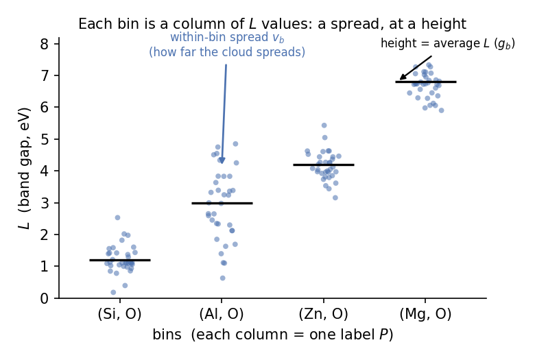
Each column is a bin; the dots are the \(L\) values in it. A column’s spread is the within-bin variation; its height is the average.
This is the picture to keep for the whole paper. (The image model looks the same: each class is a column, brightness varies within a class, and some classes — beaches — average brighter than others — coal mines.)
2.4 The audit↩︎
The working picture reduces to three numbers per bin, and producing them is one fixed procedure — an audit: take a set of outputs, sort each into its bin via \(P\) — cheap, so you bin them all — then score the expensive \(L\) on a handful of outputs from each bin (few, because \(\psi\) is dear, but enough to pin down the bin’s average and spread), and record, per bin,
its share \(w_b\) — the fraction of outputs that land in it;
its height \(g_b\) — the average \(L\) in it;
its spread \(v_b\) — how much \(L\) varies inside it.
Those three numbers per bin are the audit’s output — its shadow on \((P, L)\) — and the entire input to everything that follows. Because \(\pi\) is cheap but \(\psi\) dear, the shares \(w_b\) come out exact — you bin everything — while the heights and spreads are estimates from the scored handful: a few per bin are enough for the targets steering cares about, more when \(L\) varies mostly within bins. Application gives the rule for choosing the count, and the correction for sampling so few. You can run the very same procedure on two different sets of outputs: your training data (audit \(\mathcal{J}\)) or a batch of the model’s own samples (audit \(\mathrm{G}\)).
From here on those two terms mean precisely this — the binning and the three numbers — and the rest of the paper uses them without re-explaining.
2.5 Two ways to steer↩︎
Say you want brighter images. Here are the two moves the introduction named, now made precise — and the rest of the paper turns on the difference between them.
Telling (per-prompt steering). Work within one bin — say “golden retriever” — and lean on the controls: turn up the guidance dial, add the token “bright”, attach an adapter. You shift that bin’s outputs toward its brighter end. In the picture: you stay in one column and pull its dots toward an end.
Showing (exemplar steering). Instead of describing the target, you hand the model a batch of examples and ask for more like them. Sorted through the cheap label \(P\), that batch is a mix of bins — a recipe “70% beach scenes, 30% snow,” written \(\mu_P\). It is the mix, not the individual examples, that the move turns on, so from here we describe showing by its recipe \(\mu_P\) over bins. In the picture: you choose which columns the batch comes from.
You hand over examples, but what steers is the mix of bins they fall into — that is the one shift in vocabulary to keep. Telling works one column; showing weights different columns. They reach different parts of the picture. We make all of this precise next.
2.6 Two budgets↩︎
The total spread of \(L\) — its variance across the data — splits cleanly into the two parts the picture shows, and each move draws on one:

Telling draws on the spread within a column — the within-bin budget \(T\).
Showing draws on the spread between columns — the between-bin budget \(E\).
They sum to the whole spread, exactly:
\[\mathrm{Var}_{\mathcal{J}}(L) \;=\; \underbrace{\textstyle\sum_b w_b\, v_b}_{T\;\text{(within)}} \;+\; \underbrace{\textstyle\sum_b w_b\,(g_b - \bar g)^2}_{E\;\text{(between)}}, \qquad \bar g = \textstyle\sum_b w_b\, g_b.\]
A budget is a variance — the room available, nothing more. It says how far a property could be moved, not what any particular move does with it.
The two moves each draw on one budget. Telling reweights within a bin, so it draws on \(T\); showing reweights across bins with the recipe \(\mu_P\), so it draws on \(E\). Either way, the move shifts the average \(L\) of what you generate, and that shift is at most \(\sqrt{\chi^2\cdot\text{budget}}\) — where \(\chi^2\) measures how hard the move pushes from the original mix.
The budgets are fixed by the three numbers, before the model is built. So the deciding difference between the moves is not how hard you push but which budget each can touch at all — \(T\) for telling, \(E\) for showing. Telling cannot cross bins.
We have written the goal as the batch’s average \(L\), but it can be any property of the batch — its spread, or whether it covers two kinds at once. Theory derives the bounds, unpacks \(\chi^2\), and shows which move each kind of goal needs.
2.7 Data audit, model audit↩︎
Everything so far has audited the training data \(\mathcal{J}\) — the budget is read off the data, before the model is even built. But what you ultimately care about is what the model produces: an audit of its own outputs, \(\mathrm{G}\). So why should the data audit tell you anything about the model’s?
Because a generative model is trained to reproduce its data. For a property it reproduces well, the model’s outputs fall into the bins with the same shares, heights, and spreads as the data — the model audit matches the data audit — so the cheap data audit (no model, no sampling) stands in for it.
The catch is that the model is not trained on your property \(L\). It is trained to reproduce the data as a whole — to predict the next token, to denoise toward real samples — and \(L\) is just something you happen to care about. So the data audit stands in faithfully only when \(L\) is something the model reproduces well. A crystal generator’s density — read straight off the shape it draws — comes out matching the data; its stability — an energy that a small error in the structure throws off — does not, and there the model audit drifts from the data’s.
When you are not sure a property carries, don’t guess — check it: sample the model, audit those outputs, and compare them to the data’s bin by bin — the two numbers to read are the drift \(\delta\) (did the bin means move?) and the spread ratio \(\rho\) (did the within-bin variety carry?). Application gives that check step by step, Evidence runs it across easy and hard properties in both domains, and Theory’s Scope marks where the data audit holds and where it breaks. (A fine-tuned model reproduces a reshaped version of the data — Theory handles that too.)
Every symbol above is also collected in a one-page table, grouped by kind, in the Appendix (§A0, Notation) — for reference when a symbol turns up later without its introduction nearby.
2.8 Where to go from here↩︎
You now have the working picture — \(B\) bins of \(L\), the two moves, the two budgets. The rest of the paper builds on it in order:
Theory derives where the two square-root bounds come from, shows how the choice of recipe \(\mu_P\) scales showing’s reach (the \(\chi^2\) factor), and states the falsifiable claims that follow — then closes with a short note on what this implies for familiar training phenomena (mode collapse, the alignment tax, and the like). (It also notes why variance is the right currency — a methodological choice: cruder measures like max-minus-min are noisy.)
Evidence tests those claims in two unrelated domains.
Application turns the result into a recipe: how to measure your own budget, tell whether telling already suffices, and pick the construction that closes the gap if it does not.
A reader who wants the practice before the derivations can jump straight to Application and refer back.
3 Theory — How far telling and showing reach↩︎
Preliminaries set up the working picture and the two ways to steer. To recall: a generator \(\mathrm{G}\) produces outputs \(D\); a cheap key \(P = \pi(D)\) sorts them into \(B\) bins; the expensive target \(L = \psi(D)\) fills each bin with a spread of values; and you steer \(L\) two ways — telling stays inside one bin and nudges its outputs, while showing changes which bins the batch is drawn from. Preliminaries also named the two budgets — \(T\) (within-bin) and \(E\) (between-bin) — and their reaches. This section derives them.
§1 shows how the total spread of \(L\) splits into the two budgets. §2 derives how far each operation can move \(L\), how the recipe \(\mu_P\) scales showing’s reach through a factor \(\chi^2\), and — given a goal — which operation it calls for and, when that is showing, the shape (curvature) of the recipe it needs. §3 states the falsifiable claims that follow, including how the data-side budget transfers to a real model.
§4 then reads off what the budget implies for some familiar training phenomena, and §5 marks where the framework applies and where it stops. The detailed machinery, the case-by-case reach of each operation, and the full statement of the boundaries are in the Appendix. A practitioner can skip to Application.
Recall the per-bin quantities: bin \(b\) has share \(w_b\), mean \(g_b = \mathbb{E}_{\mathcal{J}}[L \mid P_b]\), and within-bin variance \(v_b = \mathrm{Var}_{\mathcal{J}}[L \mid P_b]\).
3.1 1. The budget: one variance, split in two↩︎
Take the property \(L\) and ask where its variation across the data lives. Some sits within bins — outputs that share a key still differ in \(L\) — and some sits between bins — different bins have different average \(L\). Those are the only two places it can live, and across the \(B\) bins they add up exactly:
\[\underbrace{\mathrm{Var}_{\mathcal{J}}(L)}_{\text{total}} \;=\; \underbrace{\sum_b w_b\, v_b}_{T\;\text{(within-bin)}} \;+\; \underbrace{\sum_b w_b\,(g_b - \bar g)^2}_{E\;\text{(between-bin)}}, \qquad \bar g = \sum_b w_b\, g_b.\]
\(T\) is the within-bin spread averaged over bins — the room telling works in, since telling stays inside one bin. \(E\) is the spread of the bin means — the room showing works in, since showing moves between bins. This identity is the law of total variance (Casella & Berger, 2002), exact for any \((\pi, L, \mathcal{J})\) — no overlap, no remainder. Its two terms are the room the two operations work in. The pieces here are elementary — the total-variance split and the Cauchy–Schwarz reweighting bound below are textbook; the contribution is not the mathematics but composing them into a cheap, pre-model, three-numbers-per-bin audit that forecasts the telling/showing crossover and, under a testable condition, carries to a trained model. And how the total divides is the practitioner’s to set through \(\pi\) — finer bins move variance into \(E\), coarser into \(T\) (at the extremes, one-output bins give \(T \to 0\); a single bin gives \(E \to 0\)) — fixing, before any model exists, which operation has room to work.
Note — the choice of variance. Why measure spread by variance rather than the range \(\max L - \min L\)? The range carries no within/between split, so it could not be divided into the two budgets at all; it is fixed by a single extreme output; and it is routinely exceeded by the model’s own outputs. Variance is the stable data-side quantity — a methodological choice, argued in full in the Appendix.
3.2 2. The two reaches↩︎
A budget is room; the reach is how far an operation can actually move the average of \(L\), given that room. Both operations move it the same way — by reweighting: shifting how much of the batch comes from where. Reweighting obeys a single law — depart from a set’s own proportions and the most you can move its average is set by how far you departed: \[|\Delta\,\mathbb{E}[L]| \le \sqrt{\chi^2 \cdot \sigma^2},\] where \(\sigma^2\) is the variance of the set you reweight and the Pearson \(\chi^2\)-divergence measures the size of the departure — \(0\) when you change nothing, growing as you pile weight onto rare values. This is Cauchy–Schwarz (derived just below). One standard deviation, \(\sqrt{\sigma^2}\), is only the gentle case \(\chi^2 = 1\); push harder and you move further, at a price that grows as \(\sqrt{\chi^2}\). The two operations differ in which set they are allowed to reweight.
Telling stays inside the bin you named. A prompt or a guidance knob can shift weight among the outputs within a bin, but it cannot move an output into a different bin — it cannot change which class, or which chemistry, the sample is. So telling reweights within bins, and the variance it acts on is the within-bin budget \(T\): \[|\Delta\,\mathbb{E}[L]| \le \sqrt{\chi^2_{\text{tell}}\cdot T}.\] Pushing the controls harder raises \(\chi^2_{\text{tell}}\), but telling is still confined to the room a bin already has. In practice the controls push gently: turning the guidance dial to its limit moves a bin’s average only a little, so \(\chi^2_{\text{tell}}\) stays small and telling’s realized reach sits near the unit-effort scale \(\sqrt{T}\) (Evidence measures it).
Showing changes the bin mix instead. Its design knob is the recipe \(\mu_P\), a distribution over the bins (Preliminaries: “70% beaches, 30% snow”). Draw bins in the data’s own proportions — \(\mu_P = \mathcal{J}_P\) — and you reproduce the data, shifting nothing; to move the average you must depart from \(\mathcal{J}_P\), drawing more from the high-\(L\) bins and fewer from the low. The shift you get is \[\Delta\,\mathbb{E}[L] = \sum_b \big(\mu_P(b) - \mathcal{J}_P(b)\big)\, g_b,\] a sum across bins of how much you over- or under-weight each bin times that bin’s average — an inner product of two lists. And an inner product is at most the product of the two magnitudes (Cauchy–Schwarz): one is how far \(\mu_P\) departs from \(\mathcal{J}_P\), the Pearson \(\chi^2\)-divergence \[\chi^2(\mu_P\|\mathcal{J}_P) = \sum_b \frac{(\mu_P(b) - \mathcal{J}_P(b))^2}{\mathcal{J}_P(b)},\] the other the spread of the bin means, \(\sqrt{E}\). So showing reweights across bins and reaches the between-bin budget \(E\): \[|\Delta\,\mathbb{E}[L]| \le \sqrt{\chi^2(\mu_P\|\mathcal{J}_P)\cdot E},\] largest when the recipe piles its extra weight on the bins with the most extreme means. The \(\chi^2\) depends only on \((\mu_P, \mathcal{J}_P)\) — never on the label.
The two reaches have the same form — \(\sqrt{\chi^2\cdot\text{budget}}\) — so the asymmetry between telling and showing lives in two other places. First, and decisively, it is structural: telling is locked to the within-bin budget \(T\) and showing to the between-bin budget \(E\), a division fixed by the key \(\pi\) before any model exists. Telling cannot reach \(E\) at all, because it cannot change bin membership — that is the heart of the matter, and it holds no matter how hard the controls are pushed. Second, it is empirical: pushed to its limit a knob departs only slightly from its bin’s own proportions (\(\chi^2\) near \(1\)), while a recipe departs sharply from the data’s mix (\(\chi^2\) of order \(100\)) — so showing realizes a far larger \(\chi^2\), and moves the mean far more (Evidence measures both).
These two halves are easy to conflate, so we separate them. The structural half is true by definition: we call an operation telling precisely when it holds the key \(\pi\) fixed — reweighting within a bin without changing bin membership — so “telling only reaches \(T\)” by definition. (Note: In one experiment in Evidence, we see that a knob pushed hard enough to rival showing turns out to leave its bin. Since it no longer is confined to a bin, we call that showing). The empirical content is the separate, non-definitional part: that real, deployed knobs realize only \(\chi^2\approx1\), two orders below a recipe’s \(\chi^2\approx100\) — and that the one knob strong enough to close the gap does so only by ceasing to hold \(\pi\) fixed, i.e. by becoming showing.
Both reaches are ceilings — computable from the bins before any model is built, and bounding the most an operation could move the mean, not predicting what it will. They come from Cauchy–Schwarz, tight only when all the weight sits on the most extreme members; a real recipe lands below, and the gap widens as \(\chi^2\) grows (Claim 2). Whether a model even delivers the in-support reach is Claim 1.
3.2.1 Which operation a goal needs↩︎
The reaches give the room; which operation claims it is the reach question. A shift small enough to find inside your bin — under \(\sqrt{T}\) — needs only telling: lean on the knobs. A larger one is out of any single bin’s within-reach, so you must show — act on the mix of bins \(\mu_P\). Telling steers within the bin you are in; it never chooses the bin.
Some goals you cannot even write down — a quality you only recognize by eye; there you show directly, letting a set of examples’ own mix of bins be the recipe (the lift; Application). For a goal you can write, one question remains once you are showing: the shape of the recipe.
3.2.2 Curvature — the shape of the showing recipe↩︎
The reach question decided whether to show; curvature decides how. Run a recipe \(\mu\) over the bins and you get a batch of outputs; the goal is some number you read off that batch — its average band gap, say, or whether it holds both a wide-gap and a stable structure. So the goal is a function \(F(\mu)\) of the recipe, maximized over the simplex \(\Delta = \{\mu \ge 0,\;\sum_b \mu(b) = 1\}\). Its curvature places the maximum:
\(F\) convex (linear included) → a vertex of \(\Delta\): concentrate \(\mu\) on one bin. Say you want the batch’s average band gap as high as possible: \(F(\mu) = \sum_b \mu(b)\, g_b\) is linear in \(\mu\), so it is largest with all the weight on the single highest-gap chemistry. A rate — the fraction of the batch past a bar — behaves the same way. That one bin is what the audit finds, so concentrating on it is still showing (reach \(E\)), not telling.
\(F\) strictly concave → the interior: spread \(\mu\) across bins. Now you want a batch that covers two kinds at once — a wide-gap structure and a stable one. No single chemistry is both; each sits in one corner, so a mix of a wide-gap bin and a stable bin holds both, and the blend beats any lone bin. Diversity behaves the same way.
Both are showing; naming the goal (telling) reaches neither. So the split — \(E\) against \(T\) — sets how far steering can move the mean; curvature sets whether the showing recipe concentrates on one bin or spreads across many.
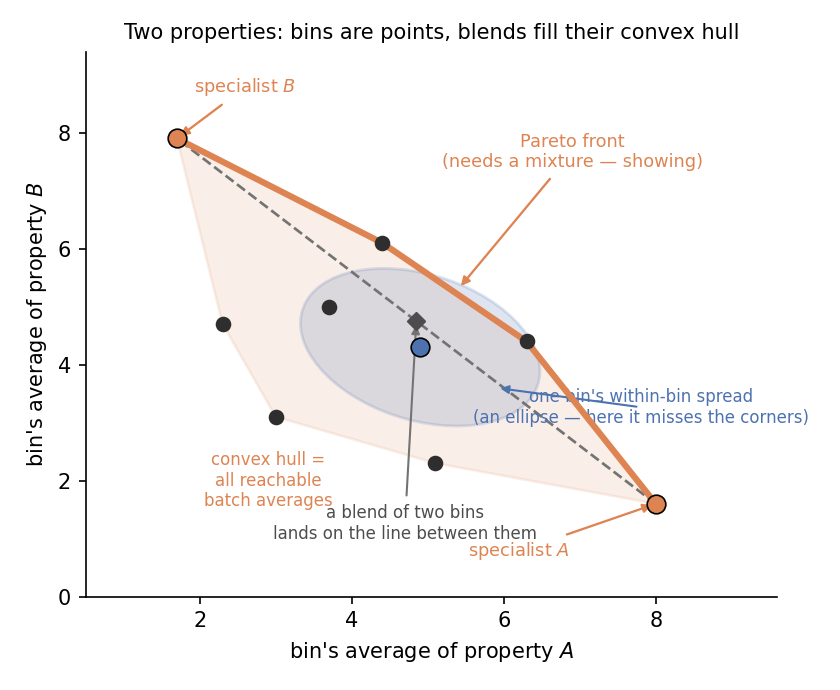
More than one property. Take two properties \(A\) and \(B\), and mark each bin as a point on a plane — its mean of \(A\) across, its mean of \(B\) up. A recipe’s batch lands at the blend of those points, so its reachable averages fill the convex hull of the bins. The goal is usually to span the Pareto front — the trade-off edge of non-dominated points — which is a coverage goal, so it needs a mixture of specialist bins (showing): a single bin is just one point on the edge. The one escape is within-bin spread — a single bin’s draws fan out into an ellipsoid, and if that reaches the front’s corners it can cover the edge alone; but the wider the front, and the more properties you stack, the less one ellipsoid reaches, so specialist bins (showing) become the only way. (The crossover, and how it tightens with the number of properties, is in the Appendix.)
3.3 3. What follows: four falsifiable claims↩︎
The framework is not vacuous; a few sharp, falsifiable claims fall out, and Evidence tests each across two unrelated domains.
The split is exact, and it carries to the model. \(T + E = \mathrm{Var}_{\mathcal{J}}(L)\) to machine precision for any \((L, \pi, \mathcal{J})\), and the split moves with \(\pi\) as described in §1. It is not only a fact about the data: for a target the model reproduces well, the model’s own outputs carry the same split, so the data-side budget describes the model too. But the model is never trained on your target \(L\) — only to reproduce the data as a whole — so a target carries faithfully only insofar as the model reproduces it, and that varies: geometry rides the training objective closely, a sharp energy loosely. Auditing a model therefore means asking how well it reproduces the particular target you chose. This is the framework’s one empirical input, which Evidence tests across easy-to-hard targets, with the diagnostics — drift \(\delta\), spread ratio \(\rho\) — read per target.
The two reaches touch orthogonal budgets — telling is confined to the within-bin budget \(T\), showing reaches the between-bin budget \(E\); each bounded by \(\sqrt{\chi^2\cdot\text{budget}}\) and computable before a model exists.
A goal’s curvature sets the shape of the showing recipe (§2). Convex/linear goals — batch averages, rates, conjunctions — peak at one bin, so showing concentrates \(\mu_P\) there (the bin the audit finds); concave goals — coverage, diversity — peak at a blend, so showing spreads \(\mu_P\) across bins, and no single bin reaches them. Both are showing; naming the goal (telling) reaches neither. For several properties at once the reachable averages are the convex hull of the bins, and covering a trade-off frontier is such a spread goal. (The Intro’s AND/OR observation, made quantitative.)
Training reshapes the budget — predictably. Plain likelihood training aims only to reproduce the data — exact for the crystal LM, a variational bound for the diffusion image model — and its objective is minimized when the model’s conditional is the data’s, so at the optimum the budget is the data’s, unchanged. Fine-tuning deliberately departs from that: filtering or RLHF reweights \(\mathcal{J}\) into a reshaped \(\mathcal{J}'\), and the new per-bin numbers are computable from the old ones and the recipe — so recompute the budget from \(\mathcal{J}'\) and you predict the tuned model’s reaches without ever sampling it. One boundary: a fine-tune can pull so far from \(\mathcal{J}\) that nothing data-side is left to recompute from — there, audit the model’s own outputs instead. (The machinery and the reshaped \(\mathcal{J}'\): Appendix.)
3.4 4. One mechanism, four phenomena↩︎
The budget also explains a familiar frustration: the harder we tune a model to score well, the more variety it loses — and the same mechanism appears to run under several named problems at once.
Take an image generator and fine-tune it for looks — the standard RLHF/DPO move. Underneath, the move is precise: it multiplies each output’s share of the distribution by a factor set by that output’s score, \[\mathcal{J}'(D) \;\propto\; \mathcal{J}(D)\, e^{R(D)/\beta},\] where \(R(D)\) is the score an output earns — here, its aesthetics — and \(\beta\) is how hard you push (smaller \(\beta\), harder push). Outputs that score well get scaled up; the rest get scaled down. (This is the same reshaped \(\mathcal{J}'\) that Claim 4 routes fine-tunes through.)
Watch what that does to our columns of bins. Within “golden retriever,” the best-looking retriever swells and the rest fade — the column narrows. Across classes, the photogenic ones (lakes, sunsets) grow while the drab ones (parking lots) shrink — the lineup of columns narrows too. Push harder (\(\beta \to 0\)) and it ends in one place: a single image, the highest-scoring one, everything else gone. Both kinds of spread have collapsed to nothing — the within-bin \(T\) and the between-bin \(E\).
And here is the crux. A reward scores one output at a time, and variety is not a property of any one output — it lives in the collection. So a per-output objective has nothing in it that can even see spread; it can only concentrate. To produce that spread you must act on the collection itself — choose the mix of bins. That is exactly what showing does: its recipe \(\mu_P\) is the only lever on the between-bin budget \(E\) from §2 — the part a per-output objective can never reach. Tuning collapses that spread; only showing realizes it.
One exception proves the rule. Objectives that score a whole set — contrastive losses, batch-diversity penalties — genuinely can reward spread. But standard RLHF and DPO do not; and even a contrastive batch is a shuffled random sample pushed apart, not a designed mix of bins — it sees a batch without choosing the collection, which is what showing does.
So one trade sits under four familiar problems — each buys per-output quality by collapsing collection spread a per-output method cannot recover:
Mode collapse — collection spread driven to the floor; the model parrots a handful of outputs.
The alignment tax — the diversity a tuned model loses is the spread it traded away for polish.
Reward hacking — hand it a reward to chase and it sprints to the single highest-scoring output.
Compositional generalization — asking for two things at once (A and B) needs outputs that already have both, and concentration only narrows. Showing can find the joint by drawing from the bins that hold it; per-output tuning never reaches it.
Read this way, the four are one mechanism wearing four names: collection-level spread that per-output training collapses and only showing restores. Each still has its own familiar driver — the architecture, the data, a badly-chosen reward — and those hold; what the framework adds is a common cause beneath all four — the between-bin spread they narrow and cannot recover, which only showing reaches; an interpretation the framework invites.
3.5 5. Scope — where this applies↩︎
We want to be precise about where the framework applies and where it does not. It applies to the mean shift of a labeled property, achieved by selection, in a model that matches its data (\(\mathcal{J}\), or the reshaped \(\mathcal{J}'\) after a standard fine-tune).
There are degenerate extremes where it does not. The bound is a forecast: a real model can fall short of it (contraction) or, off the data’s support, exceed it (expansion). And it bounds the size of a mean shift — not the literal extremes of a property, and not the value of a set-level goal like coverage or diversity. For those goals the framework still says which operation reaches them — a mixture, showing (§2) — just not how large the metric gets. The full list of edges — off-support (\(\chi^2 \to \infty\)), heavy-tailed bin means, the steered-batch variance, multi-property targets, leaving the selection regime — sits in the Appendix, each with a cheap check.
3.6 Pointer↩︎
For practical use: Application. For empirical verification of the claims: Evidence. For the shared setup and notation: Preliminaries. For the detailed machinery (data-to-model bridge), the case-by-case reach of each operation, and the full boundary statement: the Appendix.
4 Evidence — The same claims, in two unrelated domains↩︎
Theory made its predictions on paper. This section asks whether real generative models, on real data, obey them.
The theory hands us a budget: for any target, the total variation splits into a piece that telling can reach and a piece that only showing can. What we don’t yet know is whether any of it survives a real model — whether the split leaks, whether a model reaches past its budget, whether fine-tuning breaks the accounting. To keep any one result from being a quirk of a single setup, we test in two domains that share no model, no data, no labels, and no scoring code. A prediction that holds in both is hard to explain away; it reads as a property of the framework.
Vocabulary from Preliminaries: a cheap key sorts each output into a bin; the within-bin budget \(T\) is what telling reaches, the between-bin budget \(E\) what showing reaches.
4.1 The two test beds↩︎
Images — the legible track. A pretrained DiT-XL/2-256 (a diffusion model that turns a class label into an image), used as-is. The key is the class a frozen ResNet-50 reads off each image, so each of ImageNet’s 1000 classes is a bin. We steer seven plain measurements: brightness, a learned aesthetic score, compressed file size per megapixel (a stand-in for visual busyness), and four CLIP content scores — how well an image matches “a photo of an animal / a vehicle / food / nature.” You can inspect any bin’s images directly.
Crystals — the consequence track. A pretrained encoder–decoder that generates a crystal structure to meet requested properties, trained on data derived from Alexandria, a large database of computed materials. The key is chemistry — the element set and atom count, read off the output. We steer band gap, energy above hull (distance from the stability frontier; zero is stable), density, dielectric constant, and one collection-level score — Combined, the fraction of generated structures that are at once novel, unique, and at least metastable.
Cost. The image study runs in a few hours on a single GPU. The data-side claims (Claim 1, the Claim 2 bounds) are cheaper still: they need only the audit’s shadow — per-bin share, mean, and variance, 132 KB in all — and
reproduce with numpy alone, no model and no ImageNet. The companion repo ships it; verify_dataside.py checks them in under a second.
4.2 What we set out to establish↩︎
Four claims, each tested in both domains:
Figure 4: |
|
|---|---|
| The budget splits exactly, the split moves as you change the bins, and it carries to the model | |
| Telling and showing reach different parts of the budget — and we measure how much further showing reaches than a knob (bins vs knobs) | |
| An average over a batch is reached by concentrating on one bin; a spread goal only by a mix of bins — both are showing, while naming (telling) reaches neither | |
| Training changes the budget, but in a way you can predict |
 .
. The rest takes them one at a time, images first. The headline — how much further showing reaches than the best knob, and the between-bin share that says when — lives inside Claim 2, where we pit bins against the strongest knob each domain allows, property by property.
4.3 Claim 1 — The budget splits exactly, moves with the bins, and carries to the model↩︎
Three checks: the split is real, it moves with the bins, and it survives the model.
4.3.1 1. The split is exact↩︎
Total spread = spread inside the bins + spread between them, exactly.
Images, brightness, bins the 1000 classes. Total variance 0.0181; within-class (one photo in sun, another in shade) averages 0.0151; between-class (snowfields brighter than coal) 0.0030. They sum to 0.0181.
Crystals, energy-above-hull, bins the chemistry. Over 225,000 structures the total is 584 (meV/atom); within-chemistry spread is 22, between chemistries 562. They sum to 584.
This is the law of total variance, an identity — so the exact match is not evidence for anything; it just confirms we measured the three numbers right. Claim 1’s empirical weight is in the next two parts — does the split move as predicted, and does it survive the model — and in Claims 2–4.
4.3.2 2. Coarser bins shift the split↩︎
Make the bins coarser and variation moves from between to inside, as predicted.
Images: merge the 1000 classes at random into 50 — within rises 0.0151 → 0.0179, between falls 0.0030 → 0.0002, total unchanged. Crystals: drop the atom count, keep only the element set — within 22 → 120, between 562 → 464, total unchanged.
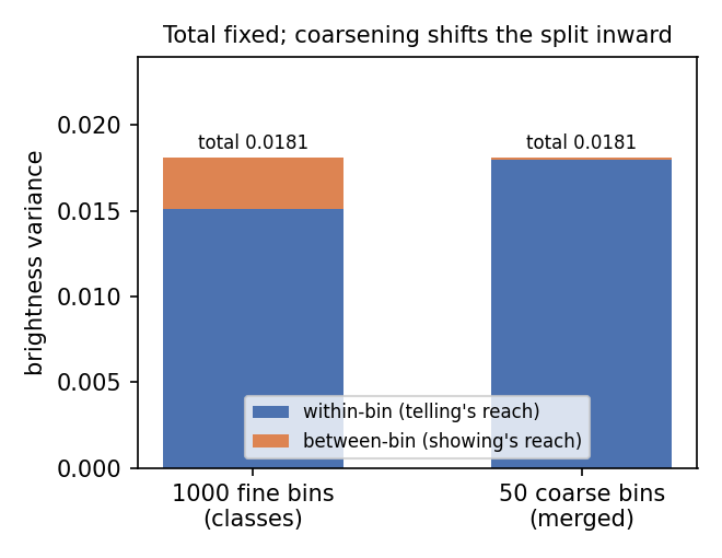
That the split moves with the bins raises a fair worry: is the budget then just an artifact of an arbitrary key? No — it tracks meaningful structure, not the bin count. Recomputing the image split under several keys, the between-bin share’s ordering across targets is stable from 1000 classes down to a structured 50-bin grouping (class-aligned targets stay high, pixel-level targets stay low); only a random 50-bin key collapses the between-bin share to near zero for every target. A structured and a random key of the same 50-bin size differ roughly eighteen-fold — so what the budget reads is the key’s structure, not its resolution. (Same on crystals: the carry-over ordering below holds across element-set and atom-count keys.)
4.3.3 3. Does the split carry through the model?↩︎
The split is a fact about the data; it matters only if the model reproduces it. A model can miss two ways: a bin lands in the wrong place (its average is off — the drift δ), or it holds the wrong amount of spread inside (the spread ratio ρ). We checked both.
Do the bin averages land where the data says? Only when the property is close to what the model was trained to produce. The model isn’t trained on these properties — the crystal model learns to get a structure’s tokens right, DiT to get pixels right — so a property comes out right only if getting the tokens (or pixels) right forces it to. Per-bin agreement (correlation between the model’s per-chemistry averages and the data’s), with 95% confidence intervals from bootstrapping over chemistries and three generation seeds:
density 0.985 [0.91, 1.00] — fixed by the structure’s shape, which the tokens fix, so it carries tightly;
bonding plausibility 0.879 [0.04, 0.97] — the intermediate rung, and its wide interval says so: the point estimate lands between density and stability as predicted, but few ionic chemistries enter its fit, so bonding alone is pinned down only loosely;
stability 0.488 [0.17, 0.71] — a few stray atoms flip a structure off the frontier, so the tokens pin it down only loosely; its agreement is both lower and far less certain.
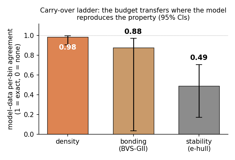
And we did not only measure this ordering — we predicted it before running the audit. From a small independent pilot, using only cheap pre-measurement signals (how often the model’s outputs even land in the data’s bins, plus the early drift δ and spread ratio ρ), we committed in advance — timestamped in the repo — to the ordering density > bonding > stability, density above ~0.9 and stability below ~0.4. The converged audit confirmed the ordering exactly (0.99 / 0.88 / 0.49); the magnitude calls were close, stability landing at 0.49 — a touch above its ~0.4 band, the one number that overshot. The ordering rests on the point estimates, which are cleanly ranked; the two ends — density high, stability low — are firm, while the middle rung (bonding) carries a wide interval and is the least certain of the three. So carry-over is a prediction the data makes ahead of time, not a pattern read off afterward — which is exactly what lets you trust the budget on a property before you have measured it on the model.
So where the agreement is high and tight — density, and brightness on images — the budget you read off the data is the one the model produces; steer by it. Where it is low and uncertain — stability — the data audit is an unreliable guide, so measure the model directly instead. And stability’s low score is the property genuinely failing to carry, not a noisy yardstick: re-scoring it with a cleaner ensemble label leaves the agreement essentially unchanged (0.42 vs 0.49), and restricting to the chemistries whose labels are most reliable does not raise it.
Does each bin hold the right variety? This is the room telling works in. On images the model produces 0.96–1.14× the data’s within-bin spread (spread ratio ρ ≈ 1), across every target — so telling’s part of the budget is real on the model, not just on paper. And the bin averages track too: for class-aligned targets — nature, animal, food — the model’s per-class means correlate with the data’s at r² 0.85–0.94 (the higher-spread brightness and aesthetic targets sit lower, 0.48–0.59, and need more samples to pin down).
The two checks are independent: one crystal model hit the right chemistries but filled them with unstable structures (high stability drift). Check both before trusting the budget on a new model.
4.4 Claim 2 — Telling and showing reach different parts of the budget↩︎
Telling reweights within a bin; showing reweights across them. Two things follow — one structural, one we measured.
Images. The experiment: take one target — the animal score — and try to move its batch average two ways, generating a batch each way and measuring how far the average moved from the model’s default. To tell, fix a class and turn classifier-free guidance up as hard as it goes (staying inside that one bin). To show, draw the batch from the classes whose animal-averages are highest. The figure plots how far each got:
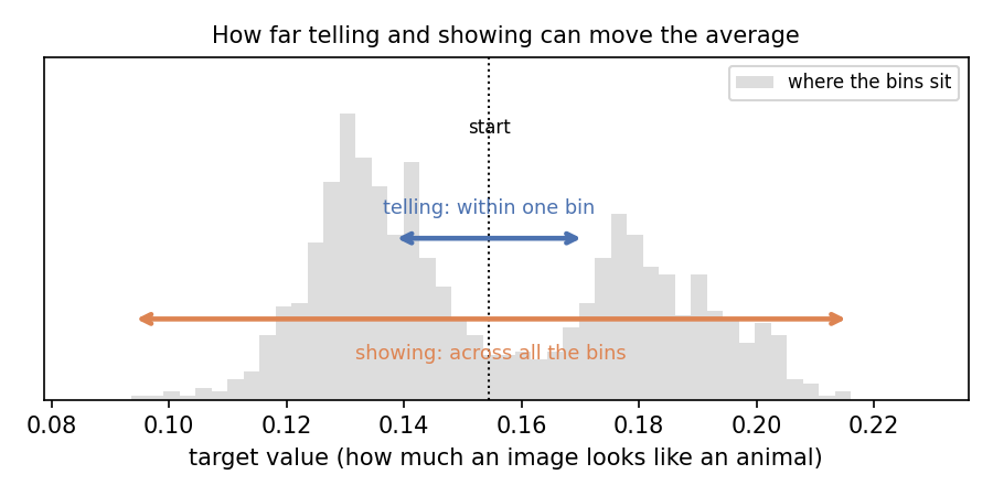
Structurally, telling cannot leave the bin it is in, so it can only reach the within-bin budget \(T\); showing moves mass across bins, so it reaches the between-bin budget \(E\). Same model, same target — different budget.
And the effort each spends differs by two orders of magnitude. We measured the χ² each operation actually puts in: telling pushed to its limit (classifier-free guidance swept up to CFG = 15) moves the within-bin distribution by a χ² of only about 1 to 1.6, while the exemplar recipes below reach χ² of order 100. At every guidance scale the realized shift stayed under telling’s own within-bin ceiling √(χ²·T) — the exact counterpart of showing’s √(χ²·E) — so √T is not a wall telling hits, just the χ² ≈ 1 scale it can afford. In one line: both obey the same √(χ²·budget) law; telling is confined to the small budget T and can spend only χ² ≈ 1, showing reaches the large budget E and spends χ² ≈ 100 — and that is the whole of the asymmetry.
Showing’s reach also grows the harder you concentrate the recipe. Drawing from the top 400, then 100, 25, and 8 of the 1000 classes, the realized shift climbed — animal score 0.031 → 0.051 (95% CI [0.029, 0.034] to [0.049, 0.053]), brightness 0.036 → 0.118 ([0.014, 0.059] to [0.085, 0.151]) — and every recipe stayed under the budget’s ceiling, √(χ²·E), with χ² measuring how far the recipe departs from the data’s own mix of bins. The ceiling rises faster than the reach, so here it is a true but loose cap: the top bins, weighted bluntly, don’t sit far enough apart to use all the room.
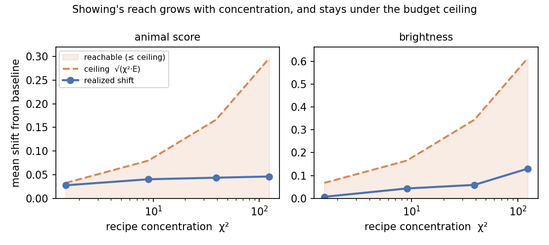
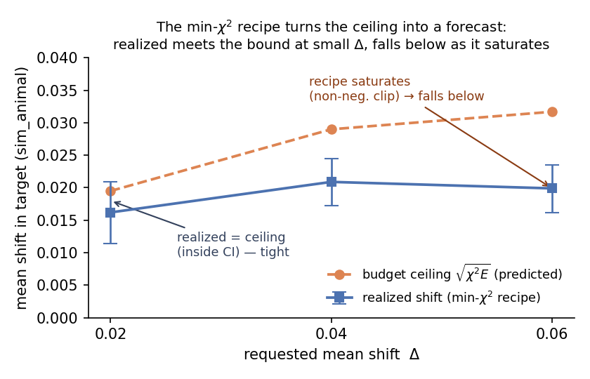
But the ceiling is loose only because the blunt top-k recipe spends its χ² inefficiently. There is a recipe that spends it optimally — the min-χ² direction, which puts exactly the bin weights the Cauchy–Schwarz bound is tight for — and there the ceiling stops being a cap and becomes a forecast. Steering one target with that recipe at a small shift, the realized move (0.0162) landed on the predicted ceiling (0.0195), inside the bootstrap CI [0.0114, 0.0209], while the blunt top-k recipe at the same χ² reached only a fraction of its ceiling. So the bound has two faces: a loose cap when you concentrate crudely, a tight prediction when you steer efficiently. (At larger shifts the min-χ² weights hit the non-negativity floor and the realized move falls back below the ceiling; the tight regime is the small-shift, in-simplex one.)
Crystals. Telling means pushing within one chemistry — there are knobs (the property-tag conditioning the model was trained with, e.g. a “high band gap” or “stable” tag, turned up like a guidance scale), but once the chemistry is fixed they barely move the result: the chemistry has already set most of what you get, and the tags only nudge within it. Showing means choosing which chemistries to draw from, and it dials the Combined score smoothly from 0.2 to 0.8 — the gap between the two reaches, as wide as the framework predicts.
4.4.1 How much further: bins versus knobs, and where the crossover falls↩︎
Start with the fair, knob-proof number. At matched effort telling can spend what it has only inside the bins and reaches at most \(\sqrt{\chi^2\,T}\); showing spends the same effort across bins and reaches \(\sqrt{\chi^2\,E}\). The common effort cancels, so their ratio is \(\sqrt{E/T}\) — fixed by the data before any knob exists, and something no knob can argue its way out of. For the three crystal targets it is 6.8 (band gap), 3.2 (density) and 1.1 (stability): effort for effort, showing reaches several times further, and most where the budget is most between-bin. That is the ceiling. What a real knob realizes is a separate question — and it is the one a skeptic presses: maybe the knobs we tried were weak. So we pushed the knob as hard as each domain allows.
Crystals. The deployed property tag is a weak knob: fix the chemistry and it realizes almost no effort (\(\chi^2\approx1\)), so the realized gap is even wider than the structural ceiling —
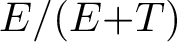
| target | \(E/(E{+}T)\) | knob shift | bin shift | realized bin / knob |
|---|---|---|---|---|
| band gap | 0.98 | 0.003 | 2.71 | ≈800× |
| density | 0.96 | 0.09 | 8.40 | ≈91× |
| stability (metastable rate) | 0.57 | 0.009 | 0.385 | ≈41× |
— every knob’s 95% CI through zero, every bin’s clear of it. (Because the knob moves essentially nothing, its CI straddling zero, the realized ratio has a near-zero denominator and is unstable — read it as “the tag does nothing,” and trust the knob-free \(\sqrt{E/T}\) column above as the equal-effort number.) But a tag is not the strongest knob a chemistry allows. The strongest is best-of-twelve: generate a dozen candidates in a fixed chemistry and keep the best by the property scorer — the largest reweighting a per-output selector can do, at matched effort \(\chi^2\approx5.3\). Even this loses, by 26× / 14× / 4.8× on gap / density / stability. On crystals the sweep holds from the weak tag all the way up to the strongest knob that stays inside a bin.
Images. Here the strongest knob is more powerful, and it changes the story — in the framework’s favour. We built a learned soft-prompt: a continuous conditioning vector warm-started at the best class and optimised directly against the target scorer, the strongest single-conditioning knob we can imagine. Against it the contest turns clean — the bin/knob ratio now rises monotonically:
Figure 10: |
Figure 11: |
Figure 12: |

|
|---|---|---|---|
| brightness | 0.29 | ||
| aesthetic score | 0.41 | ||
| vehicle content | |||
| animal content |
 .
.  .
.  .
. With a strong enough knob, two targets flip: on brightness and aesthetic — the two lowest-\(E/(E{+}T)\) scalars — the learned knob beats bins, while on the two high-share semantic targets it still loses by about three. But it wins only by leaving its bin: on those two targets the winning images land almost entirely outside the class they started from. So the experiment lets us construct a case where a knob wins, but only by breaking the bin barrier that defines telling in the first place.
One caveat keeps this honest. DiT’s guidance conditions on the ImageNet class — which is our key \(\pi\) — so on images “telling stays inside its bin” is close to true by construction, and the image contest is best read as illustration. The crystal knob is the cleaner test: the property tag (band-gap, stability) is a different handle from the chemistry key, so a tag that moves nothing while chemistry selection moves the property is genuine evidence, not a tautology of the setup. The two domains together — one where the knob and key coincide, one where they are distinct — bound the claim from both sides.
That is the whole result, stated cleanly. It is not that examples always beat knobs. \(\sqrt{E/T}\) is the fair comparison; best-of-twelve shows no within-bin knob escapes it; the soft-prompt shows the only escape is to stop being a knob — and the budget tells you, in advance, the one regime (low \(E/(E{+}T)\)) where that escape is worth making. The between-bin share is a number you read off the data before generating anything, and it names its own exceptions: brightness and aesthetic, its two lowest values.
4.4.2 Choosing the key↩︎
The whole budget is defined against a key \(\pi\) — the partition into bins — so a fair question is how to pick one without knowing the answer first. The same between-bin share answers it. Enumerate a few cheap candidate keys (a classifier’s classes, k-means over a cheap feature, element-set for crystals), and for each score \(E/(E{+}T)\) from the data alone — no generation. The key with the largest share is the one to use, and the score predicts the payoff: across candidate keys and targets, the data-side \(E/(E{+}T)\) tracks the realised bin/knob ratio (rank correlation 0.88 on images; on crystals a key-quality that also credits carry-over recovers the operative element-set key), with a structureless random partition sitting at the floor. And if no candidate key has a large share, that is itself the answer: the target is intrinsically knob-shaped — which is exactly why aesthetic and brightness, whose variance no key concentrates between bins, are the two a strong knob wins. (This needs some cheap label to bin by; discovering a key with no labels at all we leave open.)
4.5 Claim 3 — The goal’s kind sets the recipe: one bin for an average, a mix for a spread↩︎
A goal is a property of the batch you generate, and the theory splits goals in two — and with them the shape of the showing recipe. Some are an average over the batch — a high average score, a high fraction clearing a bar — and the best recipe concentrates on the single best bin (which the audit must find; it is not the average bin). Others are about the batch’s spread — the batch must cover two different kinds of output at once — and no single bin can do that, so the recipe spreads across bins. Both are showing; naming the goal (telling) reaches neither. We test both kinds, in both domains, and each needs the recipe shape the theory predicts.
4.5.1 An averaging goal: one bin wins↩︎
Start with a goal that looks like it needs a spread of bins but doesn’t. Ask for images that are both an animal and a natural scene — an otter on a riverbank — and count the fraction of the batch that clears both bars at once. That fraction is an average over the batch, so the theory says the recipe should concentrate — the single best bin should win, not a broad mix.
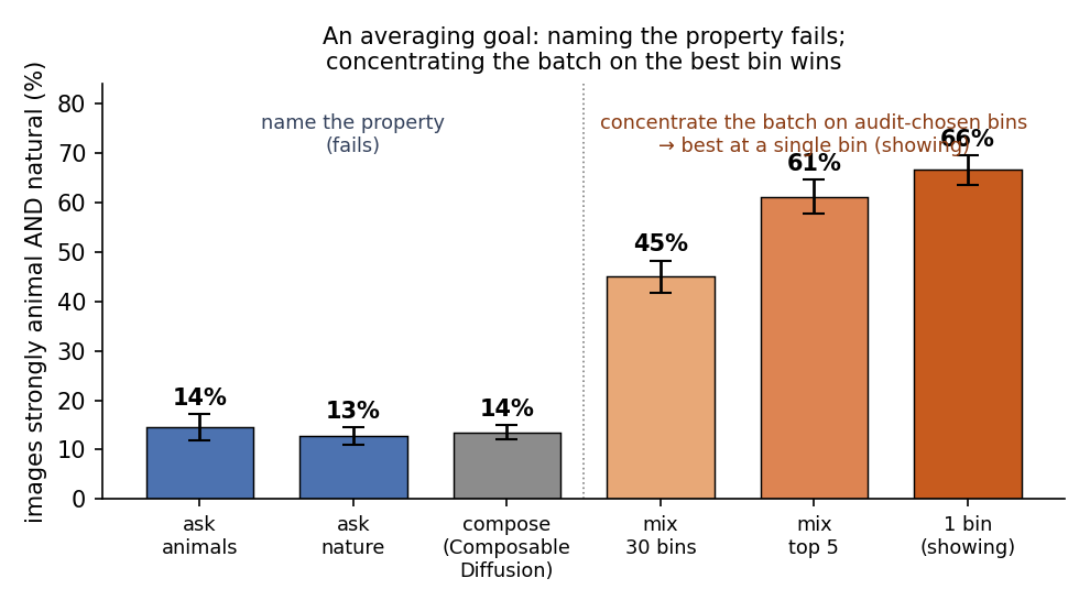
No class label is “animal in nature,” so naming the property gets you nowhere new: asking for animals, asking for nature, or composing the two with Composable Diffusion (the strongest way to compose two conditions) all land near one image in seven. But the audit points to the bins whose images are already both — otters, flamingos — and once you know them, the best move is to draw the whole batch from the single richest one (128 images per seed, ten seeds):
Figure 13: |
Figure 14: |
|
|---|---|---|
| ask for animals (naming) | % | |
| ask for nature (naming) | % | |
| compose both — Composable Diffusion | % | |
| mix 30 audit-chosen both-high bins | % | |
| mix the top 5 | % | |
| the single richest bin (showing, concentrated) | 66.5% |
 .
.  .
. Naming the property fails (~13%, Composable Diffusion — the strongest way to compose two conditions — included). Showing works, and the more concentrated the recipe the better: thirty audit-chosen bins reach 45%, the top five 61%, the single richest bin 67%. That is the averaging prediction exactly — for an average, the showing recipe should collapse onto the one best bin. It is the extreme of showing: the bin is one the audit chose (the richest, not the average bin), and a knob held inside any one bin reaches only \(\sqrt{T}\). So the conjunction never needed a spread of bins; it is an averaging goal, and a concentrated recipe — one bin — wins.
(One bin wins, but you still need the audit to find which bin — that is the showing move. Pick a class at random and crank the knob (pure telling) and you reach only \(\sqrt{T}\), the within-bin budget; the audit is what points the recipe at the right bin. And which bins pay off is itself forecastable from the audit alone, by a data-side number — the lift — with rank correlation 0.94 to the realized rates.)
The same averaging goal on crystals — a structure that is both wide-gap and stable — adds one wrinkle. Three recipes at matched sample size (joint hit = surrogate gap ≥ 3 eV and energy-above-hull ≤ 0.1; six seeds; 95% CIs):
Figure 16: |
Figure 17: |

|
|---|---|---|
| asked naively for both (telling) | % | |
| conditioned on the wide-gap prior (strong telling) | % | |
| drew from wide-gap-and-stable chemistries (showing) | % |
 .
.  .
. As an averaging goal should, one region wins. Mixing chemistries (13.2%) beats a naive request about five-fold (2.7%), but it does not beat the strong single request — conditioning on the model’s own wide-gap prior, 15.5% — the two tie (overlapping CIs, the gap holding at six seeds). Concentrating on the right region is enough; spreading does not help, exactly as for an average.
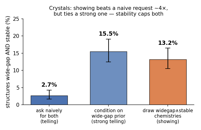
And the framework says exactly why. Showing does its job on the half it can reach — it produces the most wide-gap structures of any recipe. What caps the joint is the other half: stability sits near one in two for both showing and strong telling. Stability is the property Claim 1 found does not carry over (agreement 0.49) — the model can’t reliably make stable structures however you steer it — so it becomes the binding constraint, and the two recipes converge on it. Showing can choose the chemistry; it cannot make the model honour a property the model never learned to reproduce.
4.5.2 A goal targeting spread: only showing covers it↩︎
Now the goal the theory says genuinely needs showing: a batch that covers both corners of two properties that pull apart — some outputs clearly one, some clearly the other. Score coverage as the smaller of the two corner-fractions, so a recipe scores only if the batch holds both. We committed each prediction before running.
Images — a batch with both clean vehicles and clean food (two concepts that genuinely exclude each other, unlike animal-and-nature; 128 images per seed, five seeds):
Figure 19: |
Figure 20: |
|
|---|---|---|
| ask for one (telling, one bin) | ||
| compose both — Composable Diffusion | ||
| mix a vehicle bin and a food bin (showing) | 0.30 |
 .
.  .
. Crystals — a batch spanning the band-gap / dielectric trade-off (genuinely anti-correlated, \(-0.54\); pre-registered, three seeds):
Figure 21: |
Figure 22: |
|
|---|---|---|
| ask for one (telling, one chemistry) | ||
| condition on the wide-gap prior | ||
| mix corner-A and corner-B chemistries (showing) | 0.40 |
 .
.  .
. 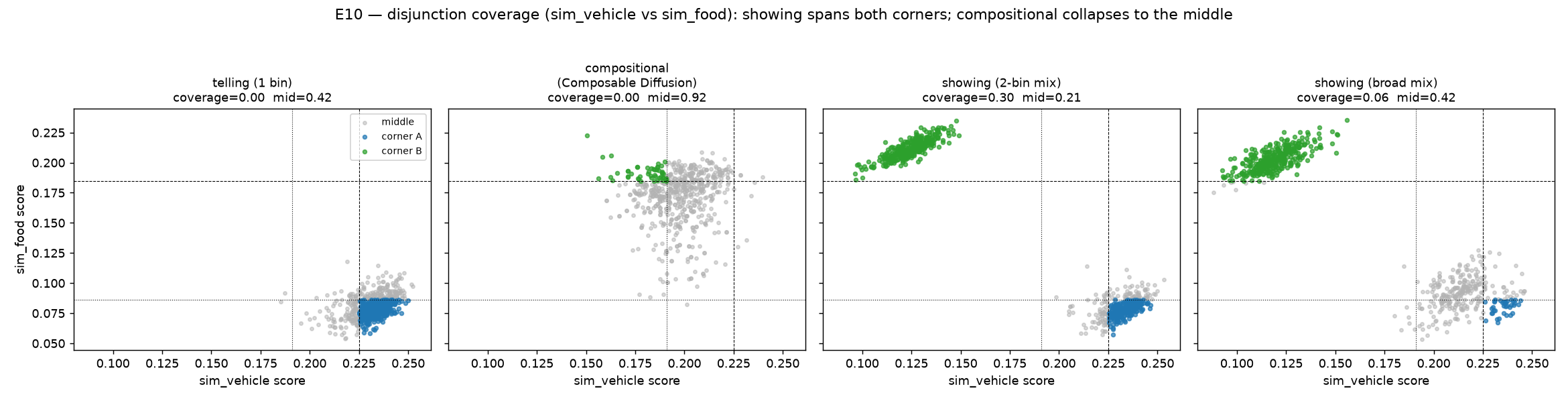
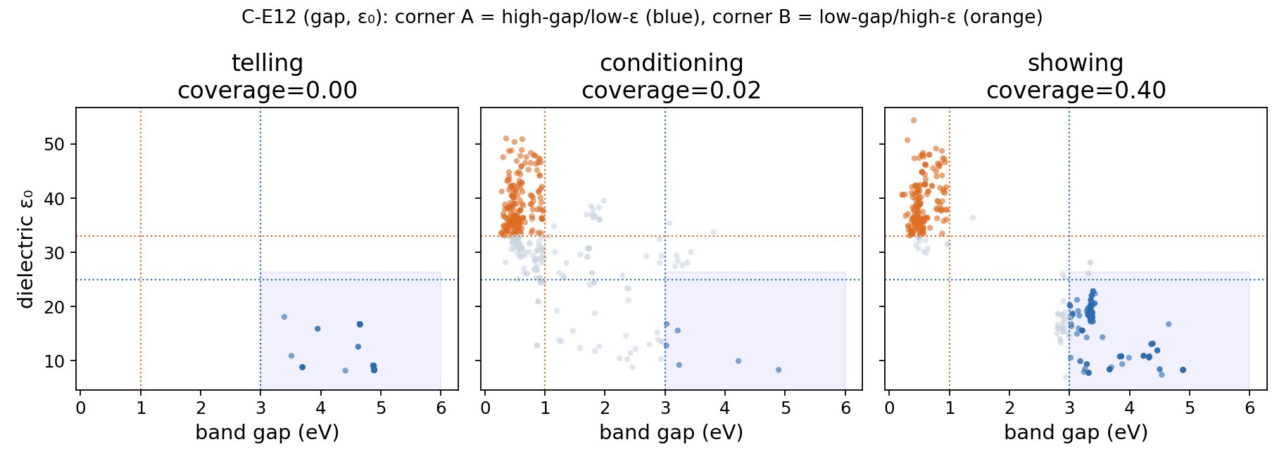
Both domains land the same way, and the two scatters tell it at a glance:
Telling sits in one corner. A single bin is all one kind, so coverage is zero by construction.
Composing the two conditions collapses to the muddy middle. Asked for “vehicle and food,” Composable Diffusion makes car-food chimeras — neither a clean car nor a clean meal (92% of the batch in the middle, coverage zero); the crystal conditioning does the same. This is the measured finding: the practitioner’s go-to tool for “both at once” returns the average, not the spread.
Showing covers both corners. A mix of a clean-corner-A bin and a clean-corner-B bin puts genuine examples of each into the batch — coverage 0.30 on images, 0.40 on crystals — the only recipe above zero, by a wide, CI-separated margin. (Precise two-corner mixing is the right recipe: the two cleanest bins cover better than a broad pool, which leaks back toward the middle.)
And the gap widens with the number of corners. Two corners is the smallest spread goal. Push to three — a batch that must hold clean vehicles, clean food, and a third clearly distinct kind at once — and the structural gap grows. Count how many corners a recipe covers with real mass (each corner’s fraction CI-separated from zero): telling covers exactly one, its own; composing conditions also covers one (its extra corners are 1–8% leakage, below any honest floor); and showing covers all \(N\) — two of two at \(N=2\), three of three at \(N=3\). The gap, showing minus telling, is \(N-1\), and it widens as you ask for more corners — the disjunctive structure of showing made quantitative: each added corner is one more bin a mix can include and a single named target cannot. (The three properties are mutually uncorrelated, so the corners are genuinely distinct, and the clean \(N=3\) test is in images. The richest crystal triple we could form was only about two-dimensional, so it tests coverage but not the \(N\)-scaling cleanly; the magnitude claim rests on the image result.)
The two crystal goals split exactly by kind. Wide-gap-and-stable is an averaging goal — you want a high fraction of the batch to be both — so the recipe should concentrate on one well-chosen region, and spreading across many adds nothing; the concentrated recipe tied the strong knob. (It tied low, not high, because stability is the property that does not carry to the model — Claim 1 — so every recipe runs into the same stability ceiling.) The band-gap/dielectric trade-off is a spread goal — the batch must cover both extremes — so only a mix of chemistries reaches it, and there showing wins outright, the same signature as images.
4.5.3 The signature↩︎
What kind of goal you have sets the shape of the showing recipe. An average over the batch wants one bin: the audit finds the best bin and the recipe concentrates on it — showing at its extreme — capped only when the property does not carry (crystal stability, Claim 1). A goal targeting the batch’s spread wants a mix: covering two corners is something no single bin can do, and composing conditions does not do it either — it returns the average. Both are showing — concentrate for an average, spread for a spread; naming (telling) reaches neither, falling short of the best bin for an average and collapsing to the middle for a spread.
4.6 Claim 4 — Training changes the budget, but in a way you can predict↩︎
Train a model only to reproduce the data and the budget is unchanged. But fine-tuning (filtering, RLHF) deliberately changes which outputs the model favours, so it changes the per-bin numbers the budget is built from — and the claim is that it changes them predictably: recompute the budget from the data and the training recipe, and you have the trained model’s budget without ever sampling it.
Plain pretraining changes nothing, so the model’s per-bin averages should match the data’s — and they do, falling on the diagonal: 0.99 agreement for crystal density, and 0.85–0.94 for DiT’s content targets, with the fit tightening as you draw more samples (at the small sample sizes we first used it was noise-limited; the high-spread targets need the most samples and stay loosest).
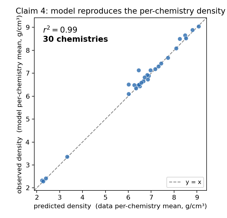
The two fine-tunes we tested each change the data in a known way; we predict the new per-bin averages from that change, then sample the model and check.
Filtering. Keep only outputs above a bar — say, crystals above a density cutoff — and the budget recomputes on the survivors. Predicted versus observed per-bin averages agreed to within 0.03 of a bin width on crystals, 0.002 on images.
Guidance. Turning up an image model’s guidance scale should shift the target’s average by a growing amount. Swept over 1, 3, 7, 12 on one class, the average climbed monotonically as predicted — animal score 0.18 → 0.20, brightness 0.52 → 0.57.
One case breaks it. Fine-tune a model so hard it abandons its training data and there is nothing left to recompute from. A crystal model fine-tuned aggressively for novelty scored real, held-out structures at −15.1 per token (95% CI [−15.2, −15.0]) — below the −9.7 of random tokens, every held-out structure without exception. For a model like that, drop the data-side prediction and audit the model’s own samples (Application shows how).
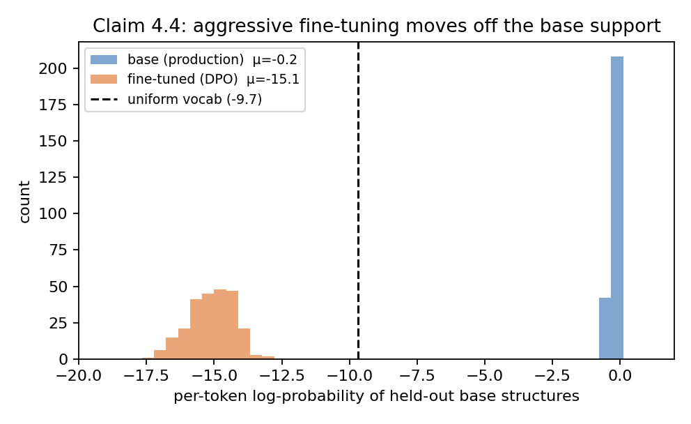
(Two more cases — mixing in supervised fine-tuning data, and distilling from a teacher — we leave for later.)
4.7 What the evidence shows↩︎
Four claims from the theory, tested in two fields that share no model, no data, and no code:
The split is exact, and it carries. The budget splits exactly; the split moves as you change the bins; and, for a property the model reproduces faithfully, it carries to the model — and we predicted which properties would carry, in advance, from cheap pre-measurement signals.
Telling and showing reach different budgets, and \(E/(E{+}T)\) says which one wins. Telling reweights within a bin, showing across them; at matched effort their reaches differ by \(\sqrt{E/T}\) (6.8 / 3.2 / 1.1 on the crystal targets), a ceiling no knob escapes. Pushed to the strongest knob each domain allows — best-of-twelve within a fixed chemistry, a learned soft-prompt optimised on the scorer — bins still beat it several-fold on every high-\(E/(E{+}T)\) target (crystals 4.8–26× at matched effort, ≈41–800× at the weak deployed tag; images ~3× on semantic content). But with a strong enough knob the low-\(E/(E{+}T)\) targets flip — brightness and aesthetic go to the knob — and the budget calls the crossover in advance: above it the range is between bins (showing); below, inside them (a knob). The winning knob wins only by leaving its bin, breaking the bin barrier that defines telling. The key \(\pi\) itself is chosen the same way — pick the cheap partition with the largest data-side \(E/(E{+}T)\) (it predicts the realised advantage, rank-correlation 0.88); a low share everywhere means the target is knob-shaped.
The goal’s kind picks the operation. An average over the batch (a high rate, a conjunction “both at once”) is reached by a single bin — telling: naming the properties fails (~one in seven on images), and the best move is to concentrate the batch on the one richest bin (67%); where the property does not carry, even that is capped (crystal stability, a tie — Claim 1). A goal about the batch’s spread — covering two opposed corners — is reached only by a mix, showing: an outright showing win in both domains (coverage 0.30 on images, 0.40 on crystals, predictions committed in advance), where telling gives one corner and composing the two conditions collapses to the average. And the spread gap widens with the number of corners: showing covers all \(N\), telling one, the gap \(N-1\) (clean \(N=3\) on images).
Training reshapes the budget, predictably. Recompute it from the data and the recipe — for plain pretraining, filtering, and guidance alike.
Two fields that share no model, data, or code land on the same answers — the exact split, the telling/showing asymmetry, the coverage win, the predictable effect of training. That is the strongest sign these are properties of the framework, not of either setup. The clearest agreement is on coverage: showing wins outright in both. The two domains differed in only one place — asking for two things at once, wide-gap and stable, was capped on crystals but not on images — and the framework named the reason in advance: a goal is capped by any property the model fails to reproduce, and stability is exactly that property (Claim 1).
What to watch for. This is also the framework’s main limitation, so it is worth collecting in one place.
The budget transfers only for properties the model reproduces well. The one place it transferred weakest was one we predicted: geometry carried almost perfectly (0.99), stability only partly and uncertainly (0.49, wide CI), because the model can’t reliably make stable structures, so there is less for its budget to come through on.
A property that does not carry caps every goal that leans on it. The same weak rung surfaced again in Claim 3: the wide-gap-and-stable goal stalled because its stability half doesn’t carry. The failure to carry over is not a footnote — it sets what any steering method can reach. (The coverage goal, on properties that do carry, was an outright showing win in both domains.)
So when in doubt, audit the model, not the data. If the property you care about may not be reproduced faithfully, score the model’s own outputs rather than the training data.
One boundary is sharper still. A fine-tune can drift so far it leaves its training distribution behind (Claim 4 — the novelty fine-tune scored real structures below random). There the data side predicts nothing at all; sample the model and audit it directly.
To put this to work on your own model, see Application; for the derivations, Theory.
4.8 Reproducing the image-domain claims↩︎
The companion repo (steering/images/) ships the audit shadow (132 KB) and the scripts, in two tiers:
Shadow only — no model, no ImageNet, no GPU.
verify_dataside.pyreproduces Claim 1 (the exact split, the \(E/(E+T)\) spectrum, the coarsening \(E\!\to\!T\)) and the Claim 2 data-side bounds, in under a second.Full regeneration — GPU + public models.
claims234.pygenerates from DiT for the model-side numbers — the realized showing shift, the per-bin averages under plain pretraining, the guidance sweep, the within-bin variety check (use ≥ 50 samples/class for the near-exact fit; the quick default of 8 is noise-limited).claim3_images.pyruns the animal-and-nature joint.
Not scripted here: the image hard-filter and the aggressive (off-data) fine-tune from Claim 4 — both need the heavier training runs, so the repo ships their results but not a one-command rerun.
5 Application — Budget, gap, and how to close it↩︎
Say you have a trained generator and you want something particular from it. Brighter images. A batch that covers the whole range from dark to bright. Crystals that are both wide-gap and stable. Or just “more like these forty I picked out.” Some of these you get by telling the model — per-prompt steering, fixing the bin and leaning on the knobs. Others you can only get by showing it: handing over examples and letting their mix steer the batch. This section tells you which, and how to build the recipe when telling isn’t enough.
It comes down to one budget and two moves. A cheap key \(P = \pi(D)\) sorts the model’s outputs into sec:bins. For the property \(L\) you want to steer, the data fixes how much room each move has: the spread within a bin is telling’s budget \(T\); the spread between bins is showing’s budget \(E\). Showing works by designing a recipe \(\mu_P\) over the bins — a distribution over bin labels, like “70% beaches, 30% snow.”
Which part you need turns on the kind of goal you have, and there are two. A single number is a level to hit: push one property’s average or rate to a target value. A shape is a pattern in the collection: two properties at once, coverage of a range, or a set you can only point to. (A goal about spread itself — a variance, a diversity score — is a single number too, but it behaves like a shape: no one bin maximizes it, so it lives with the shapes, in §3.)
A single number is §2; this is reach, the payoff of moving a property further than a knob can. A shape is §3; this is expressiveness, steering toward goals a knob cannot articulate. Most readers need one, not both. Either way, start with your per-bin numbers (§1) — off the data, or off the model itself if you don’t have the data.
5.1 1. Get your numbers (the audit)↩︎
Everything below runs on an audit (Preliminaries): the three numbers per bin — share \(w_b\), mean \(g_b\) of \(L\), spread \(v_b\) of \(L\). From them:
the within-bin budget \(T = \sum_b w_b v_b\) — the within-bin spread, averaged over bins (telling’s room);
the between-bin budget \(E = \sum_b w_b (g_b - \bar g)^2\) — the spread of the bin means (showing’s room).
Both reaches are \(\sqrt{\chi^2\cdot\text{budget}}\) (derived in Theory): telling is confined to the within-bin budget, \(\sqrt{\chi^2_{\text{tell}}\,T}\); showing reaches the between-bin budget, \(\sqrt{\chi^2(\mu_P\|\mathcal{J}_P)\cdot E}\), where \(\chi^2\) measures how hard the recipe pushes. In practice per-prompt controls realize only \(\chi^2_{\text{tell}}\approx 1\) (measured in Evidence), so telling’s working reach is about \(\sqrt{T}\) — we use that as the practical telling budget below. Showing can push \(\chi^2\) far higher, which is why it reaches so much further. You run the audit one of two ways:
Audit \(\mathcal{J}\) — you have the training data. Bin each row via \(\pi\) and summarize. (Drop bins with very few rows — say \(< 5\) — so noisy per-bin means don’t inflate \(E\).)
Audit \(\mathrm{G}\) — you only have the model. The bins are fixed by \(\pi\), so you know them before you sample. Pick a reference recipe \(\mu_P^{\text{ref}}\) to sample under (the training-time mix if you know it, else an even spread over bins, or whatever matches deployment), generate many outputs, and audit those. The identities don’t care whether the outputs came from the data or the model — the model is its own data source. Remember the \(\mu_P^{\text{ref}}\) you used; the budget depends on it.
How many to score per bin. \(\pi\) is cheap, so you bin everything and the shares \(w_b\) are exact; \(\psi\) is dear, so \(g_b\) and \(v_b\) come from a sample of \(m\) per bin. Sampling few inflates the between-bin budget — bin-mean noise reads as between-bin spread — but by a known amount, \(\hat{E} \approx E + T/m\). So calculate \(\hat{E} - \hat{T}/m\) (with \(\hat{T} = \sum_b w_b \hat{v}_b\)). Score until that correction is small against \(\hat{E}\) — if bins are small a handful is all that’s needed.
An audit is for the \(L\) you are interested in — and how far you can trust the data audit for it depends on how faithfully the model reproduces the data for that property. A generative model is trained to match its data, not to hit any one property, so it reproduces some properties closely and others loosely: a direct readout of the output — an image’s color statistics, a structure’s density — tends to carry, while a property that takes precision the model lacks, or that a separate pipeline scores — stability, an aesthetic rating — can drift. A model can be faithful on one property and loose on another, so judge this per target.
Checking that a property carries. When you are unsure, verify it directly. Because \(\psi\) is expensive, this costs a second round of scoring, but a cheap one: you are after a systematic gap, not precise per-bin values, so score \(\psi\) on a modest sample of \(\mathrm{G}\)’s outputs in just the bins your recipe leans on — a handful, not all \(B\).
Audit \(\mathrm{G}\) on that sample — sample, bin, score \(\psi\) — for the model’s per-bin mean \(g_b(\mathrm{G})\) and spread \(v_b(\mathrm{G})\). (You already have the data’s \(g_b, v_b\) from the original audit.)
Read two numbers off the comparison:
drift — the typical gap between \(g_b(\mathrm{G})\) and \(g_b\), i.e. how far the bin means moved;
spread ratio \(\rho = v_b(\mathrm{G})/v_b\) — whether within-bin variety came through (\(\rho \approx 1\) is faithful).
Turn each into a budget error. The drift is how far a showing target lands off: aim a recipe at a shift, and the model misses it by about the drift in the bins it leans on. The spread ratio rescales telling’s reach — it becomes \(\sqrt{\rho\,T}\), not \(\sqrt{T}\), so \(\rho = 0.8\) costs about 10%.
The verdict, plainly. If the drift is small next to the shift you want and \(\rho \approx 1\), the data budget is trustworthy — use \(\mathcal{J}\)’s statistics. If not, don’t lean on it: you computed \(\mathrm{G}\)’s own \(g_b, v_b\) in step 1, so build the budget from those instead.
This is the test Evidence runs (Claim 1, the carry-over check); the formal drift \(\delta\) and spread ratio \(\rho\) are defined in Appendix A.3.
Fine-tuned, not just pretrained? Still fine. A standard fine-tune (filtering, SFT, RLHF) reshapes the data into a predictable \(\mathcal{J}'\). Audit that — the same sums, on reweighted rows (table in Appendix A.1). And if the fine-tune ran so hard it left the base behind, fall back to sampling the model itself, exactly as in the sample-side path above.
Worked examples. DiT + ImageNet, target = aesthetic (DiT is a diffusion-transformer image generator; ImageNet its training set): with the ImageNet class as the key (1000 bins), an audit of 100k rows gives a substantial \(T\) (within-class variation from lighting, composition, content) and a substantial \(E\) (some classes are systematically more aesthetic). A crystal generator, target = band gap (trained on a large computed-materials database): with (elements, atom count) as the key, within-chemistry variation gives \(T\), and between-chemistry mean differences (oxides vs sulfides vs metals) give \(E\). Evidence has the full tables.
5.2 2. Hitting a target value↩︎
Say you want your batch’s average aesthetic well above what the model gives by default — or its average brightness, or its rate of “looks like an animal.” These are single-number goals: push the average (or rate) of one property \(L\) to a target. Pin it down as a desired shift \(\Delta\).
First, does telling already do it? Telling’s working reach is about \(\sqrt{T}\) — per-prompt knobs (guidance, prompt wording, an adapter) realize only \(\chi^2_{\text{tell}}\approx 1\) in practice (Evidence), so \(\sqrt{T}\) is about as far as they move the mean, whatever the model. Compare it to \(\Delta\):
\(\Delta < \sqrt{T}\) — telling suffices. Sweep your knobs and you’re done. Example: raise mean aesthetic within one ImageNet class by 0.3. Aesthetic varies a lot inside a class (utilitarian product shots to studio portraits), so \(\sqrt{T}\) comfortably covers 0.3, and a CFG sweep moves the mean there.
\(\Delta \ge \sqrt{T}\) — a gap by size. Even fully tuned, telling falls short; showing reaches further. Example: raise your batch’s mean “animal-likeness” (a CLIP similarity). That score is mostly fixed by the class, so within any one class telling barely moves it — \(\sqrt{T}\) is small. The only way to lift the batch mean is to draw more from animal-heavy classes.
To close a size gap, design a \(\mu_P\) that lands the batch mean on your target value \(g^*\) (your starting mean plus \(\Delta\)). Two ways.
Pool mixing — blend a low and a high pool. Want your batch’s average brightness somewhere in the middle? Take a pool of dark-scene classes (coal mine, night) and a pool of bright ones (beach, snowfield), and turn a single dial \(\alpha\) between them. The math is clean: sample the dark pool with probability \(\alpha\) and the bright one with \(1-\alpha\), and any collection metric linear in the mix interpolates linearly, \[\mu_P = \alpha\,\mu_P^{(1)} + (1-\alpha)\,\mu_P^{(2)}.\] What it costs: when the two pools are the bottom and top quantiles of the data (each a fraction \(q\) of the bins by mean), the push is \[\chi^2(\mu_P\|\mathcal{J}_P) \;=\; \frac{2\alpha^2 - 2\alpha + 1}{q} \;-\; 1,\] least at the midpoint, most at the extremes, and halving \(q\) doubles it — so pick the smallest \(q\) that still leaves enough distinct bins to sample without heavy repetition (\(q \gtrsim n_\text{gen}/n_\text{eligible}\)); below that, use min-\(\chi^2\).
This calibrates well in practice. On a crystal generator, mixing a high-Combined pool (rare-earth chemistries, ≈ 0.85) with a broad low one (≈ 0.14) — Combined being a novelty-and-stability benchmark — the dial tracks the target: ask for 0.5 and you get about 0.57, ask for 0.7 and about 0.73, landing within roughly 0.05 of target all the way from 0.2 to 0.8. The reachable range is set by the two pools (here ≈ 0.15–0.85); to go past either end you need a more extreme pool (§4.7).
Min-\(\chi^2\) — the gentlest push. \(\chi^2\) is how far your recipe departs from the data’s own mix, and at the same target, less departure is better: a gentler recipe wastes fewer draws on rare bins (§4.6), keeps more of the data’s diversity, and is less likely to stray off-support (§4.5). Pool mixing reaches a middling target the hard way — it piles all the weight onto the two extreme corners. Min-\(\chi^2\) reaches the same target by nudging weight onto the bins whose mean already sits near \(g^*\), and no further. That recipe — the smallest \(\chi^2\) that still hits \(g^*\) — has a closed form: \[\mu_P(P_b) \;=\; \mathcal{J}_P(P_b)\left[1 + \frac{(g^* - \bar g)(g_b - \bar g)}{\mathrm{Var}_{\mathcal{J}}(g_b)}\right], \qquad \bar g = \mathbb{E}_{\mathcal{J}_P}[g_b].\] For example, to reach \(g^* = 0.65\) it departs only a third as far as pool mixing (\(\chi^2 = 0.19\) vs \(0.60\)) — same target, gentler recipe — and comes out 3–7% more diverse. The catch: for a strict yes/no target it lands a little short (\(-0.20\) vs \(-0.11\)), because the bins near \(g^*\) hold a mix of yes and no rows. So: pool mixing for a yes/no target with well-stocked corners; min-\(\chi^2\) for a continuous target, thin corners, or diversity at a fixed target.
5.3 3. Building a shape (when no single number captures the goal)↩︎
Some goals aren’t a number at all — they’re a shape in the collection: two properties at once, coverage of a whole range, a set you can only point to. This is the expressiveness the introduction promised — goals a knob cannot articulate, the ones that matter most where naming the target is hardest. Here is why telling can’t reach them. Fix a request \(z\) (a bin plus whatever else you set) and sample: every output comes from one and the same distribution, the model’s conditional \(\mathrm{G}(\cdot\mid z)\). Telling only ever hands you that one distribution. A shape, by contrast, is a blend of distributions — and no amount of pushing turns one distribution into a blend. Only showing, mixing bins through \(\mu_P\), builds it. Three common shapes, in order below: (1) a set you can only point to, (2) two properties at once, and (3) a Pareto front to cover.
1. A set you can’t put into words — tacit steering. You’ve pulled together forty images that share a look you can’t name — a washed-out, nostalgic palette, say. You can’t write the prompt, and you have no scorer for the look, but you can point. So hand over the set: read off each image’s bin via \(\pi\), and the distribution of those bins is your \(\mu_P\). Generate from \(\mathrm{G}\) at that \(\mu_P\) — you never say what the set has in common; the bins they fall in do the steering. With no scorer, you are building \(\mu_P\) by inferring the target from the examples: the bins they crowd into stand in for the bins that score high.
But the recipe only carries which bins your examples came from, not what made each one special inside its bin. If the nostalgic palette depends on the subjects — vintage cars, faded seascapes, old storefronts — the class key sees it: \(\mu_P\) leans on those classes, and more of them is more of the look. But if the same look is a treatment that can sit on any subject — some “golden retriever” shots washed-out, others crisp, and you picked the washed-out ones — the class key can’t tell the two apart; \(\mu_P\) just says “golden retriever,” and sampling that class hands you mostly the crisp, average shot, so the nostalgic look is missed. In short: tacit steering reaches a taste the key can read, and misses one the key is blind to.
To check this you can do a free pre-check, before you generate. You can’t measure the look — no scorer — but you can ask whether the key sees it at all. Compare the examples’ bin mix \(\mu_P\) to the data’s \(\mathcal{J}_P\) with \(\chi^2\): if it is no more concentrated than a random draw of the same size — \(\chi^2\) near the floor \((B-1)/n\), for \(B\) bins and \(n\) examples — the key is blind to your taste, and a finer or different key may expose it. A \(\chi^2\) clearly above the floor means the key caught something distinctive: necessary for steering, though not proof it caught your taste rather than something that merely travels with the bins. To keep from reading signal into noise, hold out half the examples and check the concentration survives on the other half.
Which bins, not just whether. Finer than that global test, each bin’s lift — its share of your examples over its share of the data — estimates what fraction of that bin clears your bar, with no scorer at all. A small bin that soaks up many of your examples is a near-pure pocket of what you want: a 20-member bin catching ten of your top-percentile picks by chance alone would be a \(10^{-27}\) event. So lean \(\mu_P\) on the high-lift bins; Appendix B.6 gives the formula and how far to trust it.
2. A and B at once — a joint. Say a photographer wants a portfolio of specific animal-and-lighting pairings — a bright horse, a medium-lit dog, a dim cat. Each pairing is easy on its own, but there’s no clean way to ask a single prompt for “bright horse or medium dog or dim cat” at once. Showing does it directly: hand the model one example of each pairing and let those examples be the recipe — the whole portfolio in a single pass.
3. Cover a Pareto front — front expansion. Often you want two properties at their best together, where pushing one costs the other. Landscape photos that are both vivid and natural-looking, say — crank the color and it turns garish, keep it true and it falls flat — so the best you can do is a front of compromises in between. (Crystals have the same shape: a high band gap and low energy above hull.) You don’t need to know that front in advance: take a rough estimate — a few outputs near it — and build \(\mu_P\) from their bins. Sampling explores each seed bin’s neighborhood through the model’s own randomness; some outputs push past the seeds, others fill in, and the set’s Pareto volume only grows. Iterate — each round’s outputs seed the next \(\mu_P\) — and the front expands. Telling pushes one point; showing across seeds expands several at once.
Real goals often combine these — a diverse set that must also hit a joint — and the designs stack, so combine them.
5.4 4. Pitfalls↩︎
Seven practical traps bite even inside the framework’s boundaries (its theoretical edges, where the budget applies at all, are in Theory’s Scope). One line each below, in three families; the details — numbers and a check for each — are in Appendix E.
Getting the audit’s inputs right.
4.1 Raw-output discipline. Audit raw model outputs; post-processing (DFT relaxation, CFG) is a separate intervention.
4.2 Label-pipeline drift. Audit labels and evaluation labels from different pipelines produce a systematic offset.
4.3 Aggressive fine-tune. The closed-form \(\mathcal{J}'\) holds only for gentle fine-tunes; once the model has left its data, audit its own samples instead.
Where the bound loosens.
4.4 Heavy-tailed bin means. A few extreme-mean bins make the bound a loose guide, not a sharp ceiling.
4.5 Off-support \(\mu_P\). Mass on untrained bins has no prediction — \(\chi^2\) diverges to flag it.
Limits of your pools.
4.6 Thin corner pools. A tiny corner repeats itself; effective sample size collapses and \(\chi^2\) blows up.
4.7 Pool reachability. Showing only reaches between your pools; past either end you need a more extreme pool.
5.5 5. End-to-end summary↩︎
Get your numbers (§1). Per bin: share \(w_b\), mean \(g_b\), spread \(v_b\) → budgets \(T, E\). Audit the data, or the model’s own samples if you don’t have the data (report \(\mu_P^{\text{ref}}\)); fine-tuned model → audit \(\mathcal{J}'\).
Single-number goal? (§2) Compare your shift \(\Delta\) to telling’s reach \(\sqrt{T}\). Smaller → telling suffices, sweep the knobs. Larger → a gap by size; design a \(\mu_P\) to hit your target value — pool mixing, or min-\(\chi^2\) for the gentlest push.
Shape goal? (§3) Telling can’t make a shape; show one. Match it: a set you can’t describe → tacit (\(\mu_P\) from exemplars); A and B → draw from the bins that hold both; coverage → front expansion. They stack.
Generate, measure, verify the result lands inside the predicted bound — and watch the §4 pitfalls.
The setup and notation are in Preliminaries; the derivations in Theory; the cross-domain corroboration in Evidence.
6 Related work↩︎
What is new here is not the posture but the budget. Conditioning a generator on a set of examples — showing, in our terms — is an established move. Reference- and exemplar-conditioned generation (textual inversion, Gal et al. 2023; DreamBooth, Ruiz et al. 2023; IP-Adapter, Ye et al. 2023), retrieval-augmented generation (Blattmann et al. 2022), and few-shot or in-context conditioning all hand a model examples and ask for outputs like them. We claim none of that as our contribution. What this prior work does not ask is the question the budget answers: how far showing can move a target, where that reach comes from, and how it compares to what per-prompt telling can do. Our contribution is the quantitative ceiling — read off the training data before a model is built — not the act of steering by example.
Steering a generative model has been studied from many directions. We group the closest threads and say, for each, how the budget relates to it. Throughout we use the paper’s terms: telling is per-prompt steering, showing is choosing the mixture of examples to draw from, and the budget is the split of a target’s variation into a within-bin part (telling’s reach) and a between-bin part (showing’s reach). Full references are at the end of the paper.
Controllable generation. A large literature builds knobs for steering — attribute-guided decoding and plug-and-play methods for text (PPLM, Dathathri et al. 2020; GeDi, Krause et al. 2021; prefix- and prompt-tuning, Li & Liang 2021; Lester et al. 2021), and latent-direction editing for images (GAN steerability, Jahanian et al. 2020; InterFaceGAN, Shen et al. 2020). This work asks which interventions exist and how well they work in practice. We ask a prior, quantitative question: given the training data and a way to bin it, how far can any such intervention move a target — a reach you can read off the data before a model is trained. Most of these methods are telling in our terms, and the budget bounds what telling can reach.
Guidance at generation time. Classifier guidance (Dhariwal & Nichol 2021) and classifier-free guidance (Ho & Salimans 2022) push a model harder toward its condition at sampling time. Classifier-free guidance is, underneath, a reweighting of the model’s distribution toward the target — the same closed form as the fine-tunes below — which is why Claim 4 treats it as one of the predictable, training-style changes to the budget rather than a thing apart. Activation- and representation-steering — adding a learned direction to a model’s hidden states to push a behavior (the 2023–2025 line on steering vectors / activation engineering) — is the same move one level down: in our terms a within-bin knob, reaching \(T\), not \(E\), unless the added direction changes which bin the output lands in.
Fine-tuning and alignment. Reinforcement learning from human feedback (Ziegler et al. 2019; Ouyang et al. 2022), its KL-constrained optimum in closed Boltzmann form (Korbak et al. 2022), and direct preference optimization (Rafailov et al. 2023) all reshape a model’s distribution toward a reward; data filtering and rejection sampling are the blunt limit. The budget absorbs these as closed-form rewrites of the data distribution: recompute the per-bin numbers on the reshaped data and the budget carries — until a fine-tune drives the model off its data, where we stop predicting from the data and audit the model’s own samples instead.
Diversity and mode collapse. A long line of work observes that pushing a model to score well costs variety — mode collapse in GANs (Goodfellow et al. 2014; Salimans et al. 2016) — and decomposes generative quality into fidelity and diversity (precision/recall, Sajjadi et al. 2018; Kynkäänniemi et al. 2019; density/coverage, Naeem et al. 2020). The budget gives a structural reason for the trade-off: a reward scores one output at a time, so it reaches only the within-bin budget; the between-bin spread — variety across bins — is reachable only by acting on the mixture of bins, which is showing. Concretely, recall-style diversity is bounded by the between-bin share \(E/(E{+}T)\): a per-output objective, confined to \(T\), cannot buy the coverage that lives in \(E\). Mode collapse is what it looks like when an objective uses both parts up.
Exemplar and distribution steering. Choosing which bins or examples to draw from — showing — is a reweighting of the data distribution, and the mean shift a reweighting can buy is bounded by a χ²-type divergence between the chosen distribution and the data’s, a standard importance-sampling result (Owen 2013). We make that the reach of showing, paired with the between-bin budget.
Bin sampling, selection, and Pareto coverage. The structure underneath showing — allocating a budget of draws across bins — is the subject of several established literatures, whose results we borrow rather than reinvent. The within/between split is one-way ANOVA, with the between-bin fraction \(\eta^2\) the standard measure of how much a partition explains; mutual information \(I(\pi;L)\) (Cover & Thomas 2006) is its full-distribution generalization, of which our second-moment budget is the variance approximation. Whether an objective is best served by concentrating draws on one bin or spreading them across many is governed by its curvature: an objective convex in the bin allocation is maximized at a vertex (one bin), a concave one in the interior (a mixture) — the Jensen argument behind exploitation-versus-exploration in multi-armed bandits (Lattimore & Szepesvári 2020). For several properties, the achievable mean vectors are the convex hull of the bin means, and covering the Pareto front is hypervolume maximization (expected hypervolume improvement, Emmerich, Deutz & Klinkenberg 2006); coverage and diversity objectives are submodular, so greedy bin selection is near-optimal (Nemhauser, Wolsey & Fisher 1978; Krause & Golovin 2014); and matching a target output distribution is optimal transport (Peyré & Cuturi 2019). Optimal allocation for estimating a per-bin statistic — what our audit does — is classical stratified sampling (Neyman allocation; Cochran 1977). What none of these ask is our question: they select from a fixed population, whereas we steer a generative model, where the population is what the model produces and the load-bearing step is carry-over — that the model reproduces the data’s bin structure, so a budget read off the data before the model exists transfers to the trained model. The selection mathematics says what an ideal mixture could reach; carry-over is what makes it a statement about a model.
Generative models in the two test beds. For images we use a diffusion transformer (DiT, Peebles & Xie 2023) trained on ImageNet (Deng et al. 2009), with a ResNet classifier (He et al. 2016) as the binning key and CLIP/LAION models (Radford et al. 2021; Schuhmann et al. 2022) for the targets. For crystals we use a property-conditioned generator in the family of CDVAE (Xie et al. 2022) and MatterGen (Zeni et al. 2025), trained on data derived from Alexandria (Schmidt et al. 2023), with stability scored by an ML interatomic potential (MACE, Batatia et al. 2022). The two settings share no model, no data, and no code — which is the point: a prediction that holds in both reads as a property of the framework, not of either setup.
What the budget adds. Against this background, the contribution is: (1) a model-free audit that reads steerability off the training data alone, before any model exists; (2) a single split that separates two structurally different operations — telling reaches the within-bin part, showing the between-bin part; (3) the χ²-bounded reach of showing; (4) a qualitative asymmetry — some targets are reachable only by reaching across bins, not within one (showing, not telling); and (5) closed-form rewrites that carry the budget through standard fine-tuning, with an honest fallback when they break. The mathematics is standard — the law of total variance for the split (Casella & Berger 2002), Cauchy–Schwarz for the showing bound — assembled into an account of steering rather than newly derived.
7 Conclusion↩︎
We find that examples are, in general, the more powerful control: a set of examples steers a model far more strongly than its knobs, because a knob is structurally confined to part of what steering can reach. That reach is fixed before the model exists: a target’s movable range splits into a within-bin piece, which knobs reach, and a between-bin piece, which only composing examples reaches. We showed that the split is exact and tested it on two unrelated kinds of model — images and crystals — finding in both that the between-bin piece is usually the larger, so examples win, and by a lot. The advantage is not universal, and the budget says exactly when it is not.
That is reach, the measurable payoff. The second is expressiveness: because composing examples unions where a knob can only narrow, it reaches goals a knob cannot articulate — several at once, a Pareto front pushed outward, or a taste an expert can demonstrate but cannot put into words.
A familiar family of failures — mode collapse, the alignment tax, reward hacking, the failure to satisfy two requirements at once — share one cause here: each asks a per-output objective such as a per-sample reward to deliver something only a collection holds — variety, coverage, a joint. But those live between bins, beyond the reach of any per-output objective; only showing, which acts across bins, realizes them.
8 Future work↩︎
Training on collections, not rows. Per-example objectives — a likelihood, a per-sample reward — act one output at a time, so they can concentrate the between-bin budget but never enlarge it; the collection-level properties people most want (variety, coverage, joints) are invisible to them. The budget points at the fix: a training signal that scores the batch the model produces, not each sample — a distribution-level objective, the training-side analogue of showing. What such an objective would have to optimize is exactly the between-bin spread the budget measures.
Predicting carry-over from the loss. The budget carries to a model only for properties the training loss effectively constrains; we measure this after the fact. It should be predictable. The loss never sees the object directly — only the representation it scores (tokens, latents) — so a target carries to the extent the loss’s residual error leaves it untouched. A sensitivity analysis of the target against the loss’s under-constrained directions would turn the measured carry-over ladder into a predicted one. (A plain correlation of the target with the loss’s features is a first screen, but not enough: for an invertible representation it is uninformative — the loss’s weighting is what discriminates.)
Discovering the key that exposes a tacit taste. Tacit steering works only when the cheap key sorts the exemplars into bins that track the target (Application §3); when it does not, the examples scatter and \(\chi^2(\mu_P\|\mathcal{J}_P)\) sits at its random-draw floor. That floor is a scorer-free objective: search a family of keys — coarsenings, learned partitions — for one under which the exemplars concentrate well above it, pulling the taste into the between-bin budget where showing can reach. (Per bin, the lift of Appendix B.6 ranks which bins carry the target; the search is for the key that makes those lifts large.) The open problem is doing it without overfitting — \(\chi^2\) climbs trivially as the bin count approaches the number of examples, and picking the max-\(\chi^2\) key across many candidates invites spurious concentration; held-out validation is a start, a principled penalty the work. It is the same “which representation carries the target” question as the item above, asked from the key side.
The remaining training cases. Two interventions we did not test: mixing in supervised fine-tuning data, and distilling from a teacher.
A milder soft-Boltzmann checkpoint. Our aggressive novelty fine-tune left the data behind; a gentler one would test the closed-form rewrite in the regime where it should still hold.
9 Reproducibility↩︎
Every claim is backed by released code and data. The data-side audit reproduces from a 132 KB shadow of per-bin scores with numpy in under a second, no model and no GPU; the model-side checks (carry-over, realized shifts, bins-vs-knobs) run
on a single GPU in a few hours. The reproduction repository ships the image and crystal experiment scripts, the shadows, the property scorers, and per-claim verification scripts (verify_dataside.py, verify_combined.py); the
crystal generator checkpoint is hash-pinned and released separately (weights host), with every scorer’s package and version pinned in the model card. Pre-registered predictions were committed, timestamped, before the audits they forecast, and the commit
ordering is checkable in the repository history.
10 Ethics and broader impact↩︎
The framework is a measurement and steering tool, not a model: it tells a practitioner, before training, which of two existing operations will move a target property and by how much. Its risks are those of controllable generation generally — the same audit that steers toward a benign property (a material’s stability, an image’s content) steers toward a harmful one, and the between-bin reach it quantifies is the reach an adversary would also have. We see no new capability beyond what prompting and exemplar conditioning already provide; the contribution is understanding why they reach what they reach. The datasets and generators used are public research artifacts, and no human-subjects data was collected.
11 Appendix — machinery, reach, and boundaries↩︎
The Theory section keeps to three results and one implication. This appendix holds what it refers out to, so the main line stays a tight derivation:
A. the bridge from the data-side budget to a real model \(\mathrm{G}\) — the closed-form rewrites, the empirical fallback, and the diagnostics;
B. what each operation can and cannot reach, case by case;
C. the full statement of the framework’s boundaries.
It also records the methodological point deferred from Theory §1 (D, why variance, not range) and, in E, the practical pitfalls of Application §4 in full detail.
11.1 A0. Notation — symbol reference↩︎
Every symbol the paper uses, grouped by kind; this is the full table referred out from Preliminaries, where each is also introduced in plain words where it first appears. (A subscript \(b\) means “for bin \(b\).”)
Figure 27: |
Figure 28: |

|
|---|---|---|
| — the model and its outputs — | ||
| \(\mathrm{G}\) | the generator — the model that makes outputs | a picture generator; a crystal generator |
| \(D\) | one output of \(\mathrm{G}\) (sampled — ask twice, get two) | an image; a crystal |
| — reader functions — | ||
| \(\pi\) | the cheap reader → the label | image classifier; formula reader |
| \(\psi\) | the expensive reader → the target | aesthetic scorer; band-gap simulation |
| — values on an output — | ||
| \(P\) | the label \(\pi(D)\) — a key that sorts outputs into bins | “golden retriever”; (Si, O; 6) |
| \(L\) | the target property \(\psi(D)\) we steer | aesthetic, brightness, band gap |
| — bins and indices — | ||
| \(B,\;b,\;P_b\) | number of bins; a bin’s index; bin \(b\)’s label | ImageNet classes |
| — distributions — | ||
| \(\mathcal{J}\) | the distribution of your training set | “the data the model saw” |
| \(\mu_P\) | a designed recipe over bins (what showing sets) | “70% beaches, 30% snow” |
| — per-bin statistics — | ||
| \(w_b\) | a bin’s share of the data | fraction of outputs in the bin |
| \(g_b\) | a bin’s height — its average \(L\) | the bin’s mean band gap |
| \(v_b\) | a bin’s spread — variation of \(L\) inside it | band-gap variation in the bin |
| — budgets (a budget is a variance; a reweighting’s reach is \(\sqrt{\chi^2\cdot\text{budget}}\)) — | ||
| \(T\) | within-bin budget — within-bin spread, what telling draws on | reach \(\sqrt{\chi^2_{\text{tell}} T}\) |
| \(E\) | between-bin budget — between-bin spread, what showing draws on | reach \(\sqrt{\chi^2_{\text{show}} E}\) |
| — effort — | ||
| \(\chi^2\) | how hard the recipe \(\mu_P\) pushes from the data’s mix | \(1\) = mild; larger = aggressive |
 .
.  .
. 11.2 A. From the data budget to a real model↩︎
Theory §3 states the bridge: a trained model inherits the budget for the targets it reproduces (Claim 1), and a fine-tune reshapes that budget predictably (Claim 4) — both through a closed-form distribution. Here is the machinery.
11.2.1 A.1 The analytical path↩︎
The identities of Theory §1–§2 hold for any conditional distribution. At the limit of MLE training, \(\mathrm{G}(\cdot \mid z) = \mathcal{J}(\cdot \mid z)\) as full distributions, so the audit of \(\mathcal{J}\) is the audit of \(\mathrm{G}\) — for every target at once. That limit is what MLE aims at; a real model reaches it only approximately, and then the correspondence is per target: \(\mathrm{G}\) carries \(\mathcal{J}\)’s statistics for a target only as far as that target rides on the training objective (the model is never trained on the target itself). So auditing \(\mathrm{G}\) always means auditing how well it reproduces a chosen \(L\) — never \(\mathrm{G}\) in the abstract — and A.3 checks exactly that, per target. For a known training intervention, \(\mathrm{G}\) approximates an effective distribution \(\mathcal{J}'\) with a closed form — so you recompute the per-bin \(w_b, g_b, v_b\) on \(\mathcal{J}'\) (by reweighting the same rows) and every result carries over, at no new audit cost:
Figure 29: |

|
|---|---|
| MLE on \(\mathcal{J}\) | \(\mathcal{J}' = \mathcal{J}\) |
| SFT with replay \(\alpha\) | \(\mathcal{J}' = \alpha \mathcal{J} + (1-\alpha) \mathcal{J}_{\text{SFT}}\) |
| RLHF / KL-PPO with reward \(R\), penalty \(\beta\) | \(\mathcal{J}'(D \mid z) \propto \mathcal{J}(D \mid z)\, e^{R(D)/\beta}\) |
| DPO | Boltzmann form with implicit reward |
| Data filtering on \(S\) | \(\mathcal{J}' = \mathcal{J} \cdot \mathbf{1}[D \in S]/Z\) |
| Distillation | teacher distribution, optionally temperature-scaled |
 .
. 11.2.2 A.2 The empirical path↩︎
When the analytical path isn’t available — custom training, unknown parameters, or an intervention aggressive enough that \(\mathcal{J}'\) is degenerate on \(\mathcal{J}\)’s support — audit \(\mathrm{G}\) directly: measure how well \(\mathrm{G}\) reproduces the target \(L\) you care about. The same call is needed whenever \(L\) sits far from what the model was trained to match. A target the training objective subsumes — image fidelity fixes the colour distribution, fidelity being the superset — or one that neighbours it carries over from the data audit; a distant target (token likelihood says little about thermodynamic stability) does not, and must be checked on \(\mathrm{G}\)’s own samples. Audit \(\mathrm{G}\) under a stated reference \(\mu_P^{\text{ref}}\) and apply the same identities. The data-side audit of Preliminaries is just audit \(\mathcal{J}\) — and, like every audit, it is an audit of a chosen \(L\).
11.2.3 A.3 Diagnostics↩︎
When the analytical \(\mathrm{G}\) may have drifted from the empirical one, two cheap, independent checks:
Support overlap. Does \(\pi(\mathrm{G}(\cdot \mid z))\) land in \(\mathcal{J}_P\)’s bins?
Per-bin mean drift \(\delta\). Does \(g_{\mathrm{G}}(b) \approx g_{\mathcal{J}}(b)\)? \[\delta(\mu_P) = \sqrt{\mathbb{E}_{\mu_P}\!\big[(g_{\mathrm{G}}(P) - g_{\mathcal{J}}(P))^2 / v_P\big]}.\]
A model can pass one and fail the other — right bins (high overlap), wrong labels within them (large \(\delta\)). Check both. (Recipes in Application.)
11.2.4 A.4 What the model does — and doesn’t — change↩︎
The first objection the budget invites: surely a more expressive model — one that interpolates more richly between training points — produces more variance, so the budget cannot be model-independent. The intuition is right about the outputs and wrong about the budget.
A richer model walks the data manifold more densely: it emits a wider, more novel set of outputs \(D\). But the budget is the variance of a scalar property \(L = \psi(D)\), and richer interpolation fills that property’s distribution in more densely; it does not widen it. Interpolated outputs take property values between the points they interpolate — within the range already present. The only way a model enlarges \(\mathrm{Var}(L)\) is to extrapolate — emit outputs whose \(L\) falls outside the training range — which is off support (Part C).
So a model’s expressiveness shows up in two places, neither of which touches the budget:
How fully the budget is realized. Finite models drop modes and under-fill bins (contraction, \(V_{\mathrm{G}} < V_{\mathcal{J}}\)); a richer model contracts less, approaching the data-side budget from below. Expressiveness is less contraction, measured by the within-bin variance ratio \(\rho = \sqrt{T(\mathrm{G})/T}\) — a consistency check alongside \(\delta\) (\(\rho = 1\) match, \(<1\) contraction, \(>1\) expansion, the last only off support or under variance-rewarding objectives).
Output diversity itself — coverage, novelty, the size of the produced set — a non-decomposable, collection-level property (Part B). This genuinely depends on the model and is not bounded by \(\mathrm{Var}(L)\); it lives on a different axis.
In one line: richness widens the set of outputs, not the spread of a labeled property.
11.2.5 A.5 The variance of a steered collection↩︎
What is the spread of the \(L\)’s a recipe \(\mu_P\) actually produces? The same split applies, weighted by \(\mu_P\) rather than \(\mathcal{J}_P\), but with the model’s per-bin values, \[V_{\mathrm{G}(\mu)} = \sum_b \mu_P(b)\,v_b(\mathrm{G}) + \sum_b \mu_P(b)\,(g_b(\mathrm{G}) - \bar g_\mu)^2.\] Because \(\mu_P\) is a prompt distribution, this threads through the model three times — does it land outputs in the bins you asked for (support overlap), with the per-bin means and spreads the data has (\(\delta, \rho\), A.3–A.4), and are those bins in support at all? So \(V_{\mathrm{G}(\mu)}\) is exactly forecastable from the audit when the model is faithful on the bins \(\mu_P\) touches — a checkable condition — and where it is not, the data side cannot answer and you sample \(\mathrm{G}\) (A.2). If \(\mu_P\) leaves \(\mathcal{J}\)’s support, the bound announces it: \(\chi^2(\mu_P\|\mathcal{J}_P) \to \infty\), so \(\sqrt{\chi^2 E}\) goes vacuous exactly where the audit falls silent. (Note \(V_{\mathrm{G}(\mu)}\) is not capped by \(V_{\mathcal{J}}\): concentrating \(\mu_P\) on extreme-mean bins makes the collection more spread than the data — in support; what \(\sqrt{\chi^2 E}\) bounds is the mean shift, not the variance.)
A worked edge case. Take \(\mathcal{J}\), remove its two extreme-mean bins to form \(\mathcal{J}'\), and train \(\mathrm{G}\) on \(\mathcal{J}'\) — then prompt for exactly those removed bins. Since they carry no mass in \(\mathcal{J}'\), \(\chi^2(\mu_P\|\mathcal{J}'_P) \to \infty\) and the bound is vacuous: the framework makes no claim. Whether the spread of \(\mathrm{G}(\mu)\) exceeds even \(V_{\mathcal{J}}\) is then entirely up to how \(\mathrm{G}\) extrapolates — outward, and it overshoots \(\mathcal{J}\); back onto its own support, and it stays under \(\mathcal{J}'\). The framework predicts neither; it flags the regime (the diverging \(\chi^2\)) and sends you to measure \(\mathrm{G}\). The example also fixes which distribution to audit: \(\mathrm{G}\)’s reference is \(\mathcal{J}'\), the data it actually saw — auditing against the original \(\mathcal{J}\) would forecast a reach \(\mathrm{G}\) has no in-support way to deliver.
11.3 B. What each operation can reach↩︎
11.3.1 B.1 The combinatorial trap↩︎
The AND/OR observation of the Intro acquires teeth here. Telling is conjunctive: a bin specified by discrete property labels is an intersection of label values, and the number of such bins explodes exponentially in the number of properties. In practice most intersections are unrepresented in training, many were never labeled, and many interesting regions fall between named label values. So the fraction of \(\mathrm{Var}_{\mathcal{J}}(L)\) that label-based telling can actually address shrinks as property dimensionality grows. Showing has no such problem: a set of examples points at the bins that matter and needs no combinatorial coverage.
11.3.2 B.2 Telling has narrow reach↩︎
Confined to the within-bin budget \(T\): telling reweights within a bin, so its reach is \(\sqrt{\chi^2_{\text{tell}}\,T}\) — and since per-prompt controls realize only \(\chi^2_{\text{tell}}\approx 1\) in practice (Evidence), that working reach is about \(\sqrt{T}\). Stacking tokens at one bin sharpens the bin-conditional but cannot leave the bin or enlarge \(T\) — telling only moves \(L\) around within a bin’s existing spread. This is the precise form of “telling can only narrow.”
11.3.3 B.3 Decomposable vs non-decomposable metrics↩︎
Collection-level metrics split into decomposable (\(\Phi = (1/n)\sum_i \phi(D_i)\)) and non-decomposable (properties of the joint distribution of the output set). Telling can partly substitute for showing on decomposable metrics; on non-decomposable ones — set diversity, coverage, joint targets — it cannot, because there is no single-sample quantity to push.
By curvature (the full table). A goal is a property of the batch; showing shifts weight across bins via the recipe \(\mu\) (all on one bin = concentrate, many bins = spread), and the goal’s curvature decides which — convex (peaks at one bin) → concentrate, concave (peaks at a blend) → spread. Both are showing; telling (within-bin knobs) only refines the result inside whatever bin you land in. The familiar goals (each pushed up), as a function of \(\mu\):
Figure 30: |
Figure 31: |
Figure 32: |

|
|---|---|---|---|
| mean \(\mathbb{E}[L]\) | \(\sum_b \mu(b)\, g_b\) | linear | concentrate on the highest-mean bin |
| fraction over a bar \(P[L>\tau]\) | \(\sum_b \mu(b)\, r_b\) (bin rate \(r_b\)) | linear | concentrate on the highest-rate bin |
| precision (tight estimate) | \(-\mathrm{Var}\) | convex | concentrate on the lowest-spread bin |
| spread / variance | \(\mathrm{Var}(L)\) | concave | spread (mix high & low) |
| coverage of two corners | \(\min(\text{mass on }A\text{-bins},\;\text{mass on }B\text{-bins})\) | concave | spread (mix \(A\) and \(B\)) |
| diversity / # distinct | entropy | concave | spread |
| match a target distribution | \(-\) (a divergence) | concave | spread (the mixture) |
| raw extremes: max, min, range | non-smooth | via proxies: a quantile (concentrate + telling), the variance (spread) |
 .
.  .
.  .
. (Bins are sorted into corners by their mean \(g_b\) — what the audit already gives; no finer per-bin numbers are needed.) The two non-obvious rows: variance is concave because blending bins adds the between-bin term, \(\mathrm{Var}(\lambda R_1+(1{-}\lambda)R_2)=\lambda\mathrm{Var}_1+(1{-}\lambda)\mathrm{Var}_2+\lambda(1{-}\lambda)(\mu_1-\mu_2)^2\), so spread is a showing goal; distribution-matching minimizes a divergence (a quantity that bends upward), a concave goal whose best is a mixture. The raw extremes are set by a single point and do not sort by curvature; their smooth proxies do.
Multiple properties (the Pareto front). With \(N\) properties each bin is a point in \(\mathbb{R}^N\) and a recipe’s reachable means fill the convex hull. The goal — span the Pareto front of non-dominated trade-offs — is a coverage goal, so by the curvature rule it wants a mixture. The lone exception is a single bin’s within-bin spread: its \(k\) draws reach out from the mean by about \(\sigma\,\Phi^{-1}(1-1/k)\) (the expected extreme of \(k\) Gaussians), filling an ellipsoid set by the bin’s covariance; if that reaches the front’s corners, one bin covers it. The crossover is a single Mahalanobis comparison — one bin suffices iff \(\Delta\mu^{\!\top}\Sigma^{-1}\Delta\mu < [\Phi^{-1}(1-1/k)]^2\), with \(\Delta\mu\) the gap from the bin’s mean to the best specialist per property and \(\Sigma\) its within-bin covariance — so a wide front or tight bins force diversification (showing), a narrow front or loose bins allow one bin. This tilts toward showing as \(N\) grows: each added property is another corner the one ellipsoid must reach while its reach does not grow, so by \(N \gtrsim 5\) specialist bins are almost always needed (a lower bound: one bin plus one specialist per property the best bin cannot reach). Coverage is submodular, so greedy specialist selection is within \(1-1/e\) of optimal; the exact objective is the expected hypervolume improvement (EHVI; Emmerich, Deutz & Klinkenberg 2006).
11.3.4 B.4 Five cases↩︎
Each opens on the concrete instance, then states the structural reason — always the same: telling is confined to within-bin room \(T\) (reach \(\sqrt{\chi^2_{\text{tell}}\,T}\), with \(\chi^2_{\text{tell}}\approx 1\)); showing reaches between-bin room (\(\sqrt{\chi^2\cdot E}\)).
Joint targets. Image: high-aesthetic AND animal-like. Crystal: wide-bandgap AND on-hull. Telling both narrows the conditional toward zero mass — the cleanest failure. But some bins already contain joint examples, and a \(\mu_P\) on those bins reaches the joint by composition.
Tacit targets. Image: a cloud of pictures you find compelling. Crystal: materials you recognize as promising. The essence of showing: you cannot articulate the shared property, so there is no token to set. The exemplar set is the specification; the bin distribution it induces does the steering, and \(\mathrm{G}\) draws more without anyone saying why.
Non-rectangular property spaces. Crystal: the realizable manifold is not a box in property coordinates. Telling tries to reach off-manifold corners and fails; a \(\mu_P\) on bins that populate those corners reaches them.
Pareto-front exploration. Both: cover a trade-off front in two properties \(L_A, L_B\), not a point. Telling gives one point at a time; a \(\mu_P\) weighted along the front covers it by construction — a collection-level target with no single-sample analogue. (This is the one place two properties appear together; elsewhere a single \(L\) suffices.)
Properties without articulable tokens. Both: diversity, novelty, set statistics. Telling has no token to manipulate; the choice of \(\mu_P\) always exists as a knob.
11.3.5 B.5 Two honest failure modes of showing↩︎
Showing is not magic, and the formalism says where it strains.
The density problem. “More like these” assumes \(\mathrm{G}\)’s geometry agrees with what made the exemplars appealing. It may not — \(\mathrm{G}\) does not know why the set was chosen, so “near in \(\mathrm{G}\)’s sense” can drift from “appealing in the user’s sense.” This is the gap between bin membership and the within-bin detail \(T\) the user may actually care about.
The distributional-shape problem. “Variety along several axes at once” — exemplars define a cloud but not its shape along specific axes. The resolution is in the formalism: treat the exemplar set as a distribution, not a set. Want more big dogs? Supply more big-dog exemplars. The distribution of inputs shapes the distribution of outputs; the desired variety is curated in, not articulated.
Both fall straight out of the budget decomposition, and naming them sharpens the boundary of what showing buys rather than weakening it.
11.3.6 B.6 What the exemplars tell you about a bin — the lift↩︎
In tacit steering (Application §3) you build \(\mu_P\) from exemplars with no scorer. How much does that reveal about the unmeasured target? Assume only that the expert picks among the best — selection probability rises with \(L\), at overall rate \(s\) (e.g. \(s = 0.01\) for a top-centile bar). Let \(q_b\) be the fraction of bin \(b\)’s members that clear the bar. If the exemplars are a fair sample of the selected, the share landing in bin \(b\) is \(\mu_P(b) = w_b\, q_b / s\), so \[q_b = s \cdot \mathrm{lift}_b, \qquad \mathrm{lift}_b = \mu_P(b)/w_b.\] Every term on the right comes from the cheap key alone — \(w_b\) from \(\pi\) over the data, \(\mu_P(b)\) from \(\pi\) over the exemplars — so the lift estimates the fraction of a bin that clears the expert’s bar, with no \(\psi\). A small bin that soaks up exemplars has large lift and \(q_b \to 1\) (a saturated, reliable pocket); a big bin that merely contains them has lift \(\approx 1\) and \(q_b \approx s\) (the exemplars are its thin top tail). The global \(\chi^2 = \sum_b w_b(\mathrm{lift}_b - 1)^2\) is just the \(w\)-weighted spread of these lifts.
Reliability. A hard floor needs no model: the \(k_b\) exemplars in a bin are themselves selected members, so \(q_b \ge k_b/(N w_b)\) exactly (\(N\) the candidate count). The point estimate \(q_b = s\cdot\mathrm{lift}\) carries relative noise \(\approx 1/\sqrt{k_b}\) in the per-bin exemplar count \(k_b\) — one exemplar tells you almost nothing, a hundred is good to \(\sim\!10\%\). (Sampling new outputs from these bins then inherits the usual carry-over of §A.2 — \(\mathrm{G}\) must reproduce the bin’s \(L\)-distribution.)
Worked example. \(N = 10{,}000\) candidates; a bin of \(20\) (\(w_b = 0.2\%\)); all \(10\) of your top-centile exemplars land in it. The floor alone gives \(q_b \ge 10/20 = 0.5\) — half the bin clears the bar, \(50\times\) the base rate. The lift, \(1/0.002 = 500\), saturates \(q_b\) at \(1\): essentially a pure high-\(L\) pocket. Under the null (\(L\) independent of the bin) the same event has probability \((0.002)^{10} \approx 10^{-27}\).
11.4 C. Scope — the full boundary statement↩︎
Theory §5 summarizes the boundary; here it is in full. None of what follows is a hedge — each is a clean edge of a sharp claim, and almost every one comes with a cheap check that tells you which side of it you are on.
What the framework claims. The budget and its two reaches bound the mean shift of a labeled property \(L\) that can be had by selection — choosing which of the model’s behaviors to sample, whether by telling (within a bin) or showing (across bins). The claims hold when the model’s output distribution matches \(\mathcal{J}\) on the bins in play: at the MLE limit within support, or — after a standard fine-tune — against the closed-form \(\mathcal{J}'\) of A.1.
Where it stops — and what to do instead.
Off support. If the model is pushed to extrapolate, or \(\mu_P\) puts mass on bins absent from training, the data-side audit has nothing to say. The signal is built in: \(\chi^2(\mu_P\|\mathcal{J}_P) \to \infty\) and support overlap drops. There, drop the forecast and audit \(\mathrm{G}\) empirically (A.2).
Mean, not range. We bound the mean shift (and account for variances); we never claim the literal extremes. A model can produce an \(L\) past anything in training by extrapolating — off-support behavior, not a broken claim, because the min–max range was never the quantity.
Realization (the model can fall short or run over). The budget is a data-side forecast. A finite model usually falls short by contracting (\(\rho < 1\), mode-dropping); off support or under variance-rewarding objectives it can expand (\(\rho > 1\)) past the reach. The diagnostics \(\rho\) and \(\delta\) (A.3–A.4) say which.
The spread of a steered batch. \(V_{\mathrm{G}(\mu)}\) is not capped by \(\mathrm{Var}_{\mathcal{J}}(L)\) — concentrating \(\mu_P\) on extreme-mean bins makes a batch more spread than the data, in support. The reach bounds the mean shift, not the batch variance (A.5).
Heavy-tailed bin means. The showing reach is a second-moment bound; a few bins with extreme means can carry the mean shift past it. Inspect the tail before quoting it tight (Application §4.4).
Set-level targets. The reaches bound a mean. Non-decomposable, collection-level properties — diversity, coverage, joint hit-rate — are a different object (B.3); telling and showing still differ there, but the closed-form bound is for the mean.
Leaving the selection regime. Operations that don’t work by selection — gradient search on the output at inference time, say — can push \(L\) past the budget. They escape it only by leaving the regime where training data predicts behavior: a trade, not a free lunch.
Multi-property \(L\). We work one property at a time; several at once generalize through the law of total covariance (and appear together only in the Pareto case, B.4).
Non-iid generation complicates the concentration arguments for collection-level stability; the reaches hold in expectation, and a particular batch may deviate.
Practical (not theoretical) caveats — raw-output discipline, label-pipeline drift for learned-classifier labels, finite-sample audit noise — are in Application §4 (with the details in E).
11.5 D. Why variance, not range (the methodological choice)↩︎
Theory §1 uses \(\sqrt{\mathrm{Var}_{\mathcal{J}}(L)}\) as the unit of reach and notes in passing that the range \(\max L - \min L\) would be the wrong choice. In full: mean-shift reach
under controlled reweighting scales with variance, not range (that is what the Cauchy–Schwarz step gives); range has no clean within-bin / between-bin identity, so it cannot be split into the two per-operation budgets at all; and range is fragile — set by
a single extreme row, sensitive to sampling luck, and routinely exceeded by \(\mathrm{G}\)’s own outputs when the model interpolates. Variance is the stable data-side quantity. (Worked argument in
crystal_example.md.)
11.6 E. Practical pitfalls — the details↩︎
The seven traps listed in Application §4, each with its numbers and the check to run (numbered to match §4; cross-references point back to Application).
11.6.1 4.1 Audit raw outputs, not post-processed ones↩︎
Run DFT relaxation on a crystal model’s outputs before auditing them and the gap between prediction and observation jumps about fourfold. The reason: the audit describes what the model puts out, and relaxation — like CFG for images, or any refinement network — is a separate step with its own effect on the distribution. So audit and measure the raw outputs (pre-relaxation structures, images at CFG=1), and treat any post-processing as its own intervention.
11.6.2 4.2 Watch for label drift between audit and check↩︎
On DiT at CFG=1, the LAION aesthetic scorer rates the generated images about 0.44 points lower than it rated the training images — even though the model’s outputs otherwise match the data. That gap isn’t the model; it’s the scorer reacting differently to generated images than to real ones. (Brightness and CLIP-similarity labels, crisply defined, show essentially none of it.) The general trap: your prediction uses the label values recorded in the data (\(g_b\)), but your check uses whatever your evaluation pipeline computes — produce the two differently and a systematic offset appears. Crystal example: evaluating Combined, the training stability label is a DFT energy-above-hull, but the benchmark recomputes it with an ensemble of machine-learned potentials; the two disagree at the stability boundary by \(\sim 10\)pp, producing a roughly constant offset between predicted and observed Combined. Either recompute the audit with the evaluation pipeline’s labels (expensive) or report the observed-vs-predicted gap separately (the honest two-step framing). Structural labels measured the same way on both sides (brightness, density) don’t have this issue.
11.6.3 4.3 When a fine-tune is too aggressive to audit from data↩︎
A crystal model fine-tuned hard toward novelty drifted so far that it almost never produced the structures its base did — it scored held-out base structures below random chance (per-token log-probability \(\approx -17\), versus \(\approx -9.7\) for uniform). At that point there’s no use computing the budget from the original data: the model no longer resembles it. The shortcut for a fine-tuned model — rewriting it as a reweighted copy of the data (the \(\mathcal{J}'\) trick, Appendix A.1) — works only while the fine-tune is gentle enough that the model still mostly produces things the data contained. How to check: sample a few hundred outputs under your deployment recipe and see what fraction land in training bins. High (\(\ge 90\%\)): the data-based audit holds. Low (\(< 80\%\)): audit the model’s own samples instead (§1, sample-side).
11.6.4 4.4 A few extreme bins make the bound a loose guide↩︎
The showing bound averages squared deviations across bins, so it goes slack when a few bins sit far out from the rest — a heavy tail. A recipe that leans on those few bins can move the mean by much less than the averaged bound suggests, so the bound stops being a tight prediction and becomes only a ceiling. On ImageNet, brightness has exactly this shape (a handful of very bright classes), and across our concentration sweep its realized shift stayed well under the bound at every level — the ceiling held, but it was loose, rising far faster than the reach it was supposed to predict. The averaging cuts the other way too: with a heavy enough tail it carries no guarantee the realized shift won’t run over, so don’t treat it as exact. How to check: before quoting the bound as tight, look at the spread of bin means; if a handful dominate, read it as a loose guide, not a sharp number.
11.6.5 4.5 Recipes that wander off the training data↩︎
Build a \(\mu_P\) that puts real weight on bins the training set never contained, and the budget has nothing to say there — it was computed from data that doesn’t cover that ground. Usefully, the \(\chi^2\) factor announces this itself: it blows up as \(\mu_P\) puts mass where the data had none, so the bound \(\sqrt{\chi^2 E}\) goes vacuous right at the edge of support. Fix: whenever you build a \(\mu_P\), check how much of its mass lands on training bins; if a meaningful share is off-support, drop those bins and renormalize, or flag those outputs as outside the framework.
11.6.6 4.6 Thin corner pools repeat themselves↩︎
Aiming at a target \(g^* = 0.35\) from a corner of only 20 bins (64 rows), a pool-mixing design drew 35 prompts but got only 87 distinct ones out of 100 — the same few bins kept coming up. With so little to draw from you effectively have far fewer independent samples (here 73.5, not 100), and the push \(\chi^2\) shoots up to 52.3, two orders of magnitude above a healthy pool — predictable from \(\chi^2 \approx 1/q - 1\). How to check: compute the floor \(q \gtrsim n_\text{gen}/n_\text{eligible}\); below it, switch to min-\(\chi^2\), which borrows from the middling bins to recover independent samples, at some cost in precision.
11.6.7 4.7 You can only reach as far as your pools↩︎
Showing steers between the extremes your pools provide. With a high pool at Combined ≈ 0.85 and a broad low one at ≈ 0.14, the reachable range is about 0.15 to 0.85: ask for 0.1 and you saturate at ~0.15, ask above 0.85 and there is nothing to mix toward. To widen the range you need a more extreme pool — if the data holds one. (More deeply, a real model carries its data’s statistics only in the ideal limit (Theory, Claim 1), so its reachable range can sit inside the data-side bound; past that, the bound over-promises.) How to check: measure your two anchor pools’ scores first — that bracket is your range.
12 References↩︎
Batatia, Kovács, Simm, Ortner, Csányi. “MACE: Higher Order Equivariant Message Passing Neural Networks for Fast and Accurate Force Fields.” NeurIPS 2022.
Blattmann, Rombach, Oktay, Müller, Ommer. “Retrieval-Augmented Diffusion Models.” NeurIPS 2022.
Casella, Berger. Statistical Inference, 2nd ed. Duxbury, 2002.
Cochran. Sampling Techniques, 3rd ed. Wiley, 1977.
Cover, Thomas. Elements of Information Theory, 2nd ed. Wiley, 2006.
Dathathri, Madotto, Lan, Hung, Frank, Molino, Yosinski, Liu. “Plug and Play Language Models: A Simple Approach to Controlled Text Generation.” ICLR 2020.
Deng, Dong, Socher, Li, Li, Fei-Fei. “ImageNet: A Large-Scale Hierarchical Image Database.” CVPR 2009.
Dhariwal, Nichol. “Diffusion Models Beat GANs on Image Synthesis.” NeurIPS 2021.
Emmerich, Deutz, Klinkenberg. “The Computation of the Expected Improvement in Dominated Hypervolume of Pareto Front Approximations.” Technical Report, Leiden University, 2006.
Gal, Alaluf, Atzmon, Patashnik, Bermano, Chechik, Cohen-Or. “An Image is Worth One Word: Personalizing Text-to-Image Generation using Textual Inversion.” ICLR 2023.
Goodfellow, Pouget-Abadie, Mirza, Xu, Warde-Farley, Ozair, Courville, Bengio. “Generative Adversarial Nets.” NeurIPS 2014.
He, Zhang, Ren, Sun. “Deep Residual Learning for Image Recognition.” CVPR 2016.
Ho, Salimans. “Classifier-Free Diffusion Guidance.” arXiv:2207.12598,
Jahanian, Chai, Isola. “On the ‘Steerability’ of Generative Adversarial Networks.” ICLR 2020.
Korbak, Perez, Buckley. “RL with KL Penalties is Better Viewed as Bayesian Inference.” Findings of EMNLP 2022.
Krause, Golovin. “Submodular Function Maximization.” In Tractability: Practical Approaches to Hard Problems, Cambridge UP, 2014.
Krause, Gotmare, McCann, Keskar, Joty, Socher, Rajani. “GeDi: Generative Discriminator Guided Sequence Generation.” Findings of EMNLP 2021.
Kynkäänniemi, Karras, Laine, Lehtinen, Aila. “Improved Precision and Recall Metric for Assessing Generative Models.” NeurIPS 2019.
LAION. “LAION-Aesthetics.” laion.ai/blog, 2022.
Lattimore, Szepesvári. Bandit Algorithms. Cambridge UP, 2020.
Lester, Al-Rfou, Constant. “The Power of Scale for Parameter-Efficient Prompt Tuning.” EMNLP 2021.
Li, Liang. “Prefix-Tuning: Optimizing Continuous Prompts for Generation.” ACL-IJCNLP 2021.
Naeem, Oh, Uh, Choi, Yoo. “Reliable Fidelity and Diversity Metrics for Generative Models.” ICML 2020.
Nemhauser, Wolsey, Fisher. “An Analysis of Approximations for Maximizing Submodular Set Functions—I.” Mathematical Programming 14:265–294, 1978.
Ouyang, Wu, Jiang, Almeida, Wainwright, et al. “Training Language Models to Follow Instructions with Human Feedback.” NeurIPS 2022.
Owen. Monte Carlo Theory, Methods and Examples. 2013.
Peebles, Xie. “Scalable Diffusion Models with Transformers.” ICCV
Peyré, Cuturi. “Computational Optimal Transport.” Foundations and Trends in Machine Learning 11(5–6):355–607, 2019.
Polanyi. The Tacit Dimension. Doubleday, 1966.
Radford, Kim, Hallacy, Ramesh, Goh, Agarwal, et al. “Learning Transferable Visual Models From Natural Language Supervision.” ICML
Rafailov, Sharma, Mitchell, Ermon, Manning, Finn. “Direct Preference Optimization: Your Language Model is Secretly a Reward Model.” NeurIPS
Ruiz, Li, Jampani, Pritch, Rubinstein, Aberman. “DreamBooth: Fine Tuning Text-to-Image Diffusion Models for Subject-Driven Generation.” CVPR 2023.
Sajjadi, Bachem, Lucic, Bousquet, Gelly. “Assessing Generative Models via Precision and Recall.” NeurIPS 2018.
Salimans, Goodfellow, Zaremba, Cheung, Radford, Chen. “Improved Techniques for Training GANs.” NeurIPS 2016.
Schmidt, Hoffmann, Wang, Borlido, Carriço, Cerqueira, Botti, Marques. “Machine-Learning-Assisted Determination of the Global Zero-Temperature Phase Diagram of Materials.” Advanced Materials 35(22):2210788, 2023.
Schuhmann, Beaumont, Vencu, Gordon, Wightman, et al. “LAION-5B: An Open Large-Scale Dataset for Training Next Generation Image-Text Models.” NeurIPS 2022 Datasets and Benchmarks Track.
Shen, Gu, Tang, Zhou. “Interpreting the Latent Space of GANs for Semantic Face Editing.” CVPR 2020.
Xie, Fu, Ganea, Barzilay, Jaakkola. “Crystal Diffusion Variational Autoencoder for Periodic Material Generation.” ICLR 2022.
Ye, Zhang, Liu, Han, Yang. “IP-Adapter: Text Compatible Image Prompt Adapter for Text-to-Image Diffusion Models.” arXiv:2308.06721, 2023.
Zeni, Pinsler, Zügner, Fowler, Horton, Fu, et al. “A Generative Model for Inorganic Materials Design” (MatterGen). Nature 639:624–632,
Ziegler, Stiennon, Wu, Brown, Radford, Amodei, Christiano, Irving. “Fine-Tuning Language Models from Human Preferences.” arXiv:1909.08593, 2019.