TEDDY: A Pediatric Foundation Model for Risk Forewarning from ICD-Coded Diagnostic Histories
July 15, 2026
Abstract
Pediatric electronic health records capture developmentally structured clinical trajectories, yet their potential for generative healthcare foundation models remains largely unexplored. Here we present TEDDY (Temporal Event Decoder for Disease in Youth), a 1.84-million-parameter decoder transformer trained on approximately 73 million ICD-10 diagnoses from 1.6 million children at a single pediatric institution. TEDDY models longitudinal diagnosis trajectories and visit timing. Predictions were made before visit codes were revealed, limited to first occurrences, and evaluated against sex- and age-matched controls. Across 797 disease-onset prediction tasks spanning 16 ICD-10 chapters, TEDDY achieved a median AUC of 72.0%, outperforming same-data DenseNet (50.0%), CNN (57.2%), RNN (60.1%), and LSTM (62.7%) baselines on 96–99% of tasks. Performance held across sex and age and was strongest among lower-prevalence diagnoses; 202 of the 225 rarest conditions (90%) had 95% confidence intervals above chance. Predictive signal remained detectable more than two years before first recorded diagnosis, with median AUCs of 59.7% in the unrestricted analysis and 64.4% in a fixed-cohort sensitivity analysis. In asthma and attention-deficit/hyperactivity disorder benchmarks, AUCs were 79.3% and 84.7%, compared with 62.7% and 71.7% for the strongest comparators, including a general-purpose language model three orders of magnitude larger. Visit-timing predictions had a 3.0-day mean absolute restricted mean survival-time error over 365 days, although median and long-tail return intervals remained miscalibrated. Together, these results establish pediatric diagnostic histories as a substrate for compact generative models supporting broad, rare-disease, and long-horizon risk forecasting without population-scale data or billion-parameter models.
1 Introduction↩︎
Pediatric patients differ from adults anatomically, physiologically, and in disease presentation, yet most clinical prediction tools are trained on adult data [1]. Doses, normal vital-sign ranges, and even the appearance of illness are age-dependent, so that sepsis in a premature newborn looks nothing like sepsis in a teenager [2]. Because clinical evidence is generated largely in adults, the protocols, practice guidelines, and therapies derived from adult data cannot be applied directly to children — pediatric prescribing, for example, still leans heavily on off-label use [3], [4]. The same limitation now extends to the artificial-intelligence and machine-learning (AI/ML) tools poised to reshape clinical care: only 17% of FDA-approved AI/ML devices are labelled for pediatric use [5], [6], and of 181 public medical-imaging datasets, just 3.3% are pediatric-only, with a further 14.4% mixing adult and pediatric data [5]. Models trained mostly on adults can misread the physiology of children and return unreliable predictions for the very patients they are meant to help.
The case for models built specifically for children rests on a simple fact: the pediatric disease landscape is not a smaller version of the adult one. Two classes of condition make the point. The first is developmentally specific disease that has no adult counterpart — congenital and genetic disorders, complications of prematurity, and neurodevelopmental conditions such as autism spectrum disorder — which arise from and unfold along the biology of early development [7], [8]. The second is disease that clusters in childhood, such as asthma, allergy, and epilepsy, where adult records are neither complete nor representative of how the condition first presents and evolves in a child. In both classes, a model trained on adult data inherits the wrong priors.
Rare disease sits at the sharp end of this second class and carries the heaviest burden. Rare conditions are disproportionately pediatric in onset [9], and families spend more than six years on average in search of a diagnosis [10]–[12], at an estimated $86,000–$517,000 per patient — a burden that reached $997 billion in the United States in 2019 [13]. Conventional decision-support tools are not built to track illness that shifts with development [2], [14], so this diagnostic odyssey persists even where the clues accumulate in the record. Pediatric-specific, data-driven medicine offers a way forward. A child’s clinical trajectory is shaped by rapidly changing developmental physiology, age-specific disease prevalence, preventive-care schedules, and close links between maternal, infant, and early-life records, so a clinically useful model must recognize not only what has already occurred in a child’s record but also what may emerge next as the child develops. Surfacing that trajectory at any encounter that raises concern — in the emergency department, in urgent care, or at a specialty referral — could prompt earlier testing, referral, or admission before acute deterioration, bring appropriate intervention forward, and cut the cost of a missed rare diagnosis. Yet open-vocabulary forecasting across the broad range of pediatric diagnoses remains largely unexplored.
The methods that might fill this gap were developed almost entirely in adults, where transformers have been shown to learn disease trajectories from longitudinal EHRs along two lines (Table 1). The first adapts BERT-style models — BEHRT [15], Med-BERT [16], CEHR-BERT [17], and Hi-BEHRT [18] — which learn bidirectional representations and then fine-tune a classifier for one task at a time, such as heart-failure readmission or diabetes onset. Because they are discriminative, these models do not generate future events and are often tested on a handful of hand-picked conditions rather than across the whole diagnostic range.
The second line is autoregressive and generative: it treats a patient’s history as a sequence of tokens and predicts the next medical event, and when it will occur. Delphi [19] adapts GPT-2 with a continuous age encoding and an exponential waiting-time head, training on 0.4 million UK Biobank participants to predict the onset of more than 1,000 ICD-10 diagnoses. ReClaim [20] scales the approach to 43.8 billion events from over 200 million enrollees in a commercial-claims database, adds procedures, medications, and cost, and reaches a mean AUC of 75.6% across more than 1,000 disease-onset tasks. Epic’s Curiosity [21] shows the same models improve with scale, training Qwen2 decoders of up to one billion parameters on 118 million patients from Epic Cosmos. Others — Foresight [22], MOTOR [23], TransformEHR [24], and Life2vec [25] — vary in architecture and data but share the insight that autoregressive pretraining over clinical sequences captures temporal structure that discriminative classifiers miss.
Two methodological pitfalls can make reported performance look better than it is. The first is within-encounter leakage. EHR systems record diagnoses only to the calendar day, so the several codes billed on one visit carry no order among themselves. When a model is scored by predicting each code in turn under a standard causal mask, a code can be predicted from its same-day neighbours — diagnoses that were not yet known when the visit began. If asthma (J45) and pneumonia (J18) are billed the same day, such a setup can let the model use the asthma code to predict the pneumonia code, inflating apparent accuracy. How much this bites depends on how a model handles a visit: approaches that generate or score a whole visit at once, or that condition on a known reason for the encounter, are exposed differently. The second pitfall is demographic confounding. If a sex-specific condition — say endometriosis or testicular torsion — is scored against a mixed cohort, most of the comparison group is of the opposite sex and trivially easy to tell apart, so the model scores well on demographics alone rather than on any clinical signal. Designing training and evaluation so that a model learns real predictive structure, instead of exploiting either shortcut, is a central methodological challenge.
These adult models also leave a population gap. Almost every generative EHR model has been trained on adults or mixed-age cohorts. Notably, Curiosity excluded children outright, reasoning that pediatric care differs too much from adult care, while naming pediatrics — with its maternal and infant links, developmental physiology, vaccination schedules, and congenital timelines — as a promising, unaddressed frontier. Claim-PT [26] is, to our knowledge, the only transformer pretrained on pediatric claims, but it is encoder-only and was evaluated on specific tasks rather than open-vocabulary forecasting — so the generative paradigm has not yet been brought to children.
Pediatric records also differ in clinical structure. Childhood care is organized around developmental transitions, preventive visits, immunizations, developmental surveillance, and the early manifestations of congenital and genetic disease [7], [8], [27], [28], and the same diagnosis can carry different prevalence, implications, and expected timing at different ages [29]. Well-child and vaccination visits can dominate a longitudinal record without reflecting disease progression, while maternal and infant histories that carry important context are often held in separate records. A pediatric model must therefore separate routine developmental care from evolving clinical risk while staying sensitive to conditions that emerge within narrow developmental windows.
Data availability compounds these obstacles. Public pediatric EHR data are scarce — large biobanks such as the UK Biobank [30] and MIMIC-IV [31] are overwhelmingly adult — and the pediatric records that do exist are fragmented across systems [32]. Children with complex conditions are seen only intermittently at major centers, while most of their care happens with community providers whose records rarely reach those centers, so any one institution sees only a truncated, unevenly sampled slice of each child’s story. The road to stronger performance in adult EHR modelling has run through ever-larger datasets and models — a road largely closed to individual pediatric institutions, which must instead learn from carefully curated, comparatively small data.
Meeting these challenges calls for a model whose predictions can be trusted on the conditions that matter most — which depends as much on how it is evaluated as on how it is built. We present TEDDY (Temporal Event Decoder for Disease in Youth), a decoder transformer that reads a child’s unfolding medical story and flags what may be coming — like an attentive pediatrician with perfect recall of every similar child seen before. TEDDY is trained with a joint next-code and time-to-event objective on 1.6 million patients and approximately 73 million ICD-10 diagnoses from the pediatric EHR of Texas Children’s Hospital (TCH).
We make three design choices in response: two close the shortcuts above, and one keeps the task clinically meaningful. First, a visit-structure representation brackets the codes of each same-day encounter and scores every new diagnosis at the visit boundary — before any of that day’s codes are revealed — removing within-encounter leakage while keeping a standard causal model. Second, we match each case to controls of the same sex and similar age, so that per-condition accuracy reflects clinical signal rather than demographics. Third, we score each condition only at its first occurrence, so the task is anticipating a genuinely new diagnosis rather than re-predicting one a child already carries. We then ask how far in advance each diagnosis can be anticipated, reporting accuracy from the same day out to two or more years in advance.
Trained on the full ICD-10 vocabulary across all 22 chapters, TEDDY reaches a median first-occurrence AUC of 0.72 on the 797 conditions (validated across 16 disease-bearing chapters) that meet our thresholds. That accuracy holds across sex and age and is, if anything, strongest for the rarest conditions. At just 1.84 million parameters it outperforms four other sequence architectures and a general-purpose language model three orders of magnitude larger. The signal is readable years before a diagnosis is recorded, and the model’s timing estimates agree with observed timing at the decile level, though it miscalibrates both typical and long-tail return intervals. Together these results give the first generative EHR foundation model built for children, and show that careful trajectory representation and rigorous evaluation can yield clinically meaningful predictions even in the small-data, long-tailed world of childhood disease.
| Model | Architecture | Enc/Dec | Pre-training Objective | Data Source | Population | Event Types | Model Size | Code Recurrence |
|---|---|---|---|---|---|---|---|---|
| Delphi-2M [19] | GPT-2 | Decoder | Autoregressive + Time-to-event | UK Biobank (0.4M) | Adult | Dx, death, lifestyle | 2.2M | No |
| ReClaim [20] | Qwen3 | Decoder | Autoregressive + post-training | MarketScan Claims (200M) | Adult | Dx, Rx, Px, cost | 140M–1.7B | Yes |
| Curiosity [21] | Qwen2 | Decoder | Autoregressive | Epic Cosmos (118M) | Adult | Dx, Rx, Px, labs | 62M–1B | Yes |
| BEHRT [15] | BERT | Encoder | Masked Language Modeling | CPRD (1.6M) | Adult (Mixed) | Dx | Not reported | No |
| Med-BERT [16] | BERT | Encoder | Masked Language Modeling | Cerner (28M) | Adult | Dx | 17M | No |
| CEHR-BERT [17] | BERT | Encoder | Masked Language Modeling + Visit Type Prediction | CUIMC-NYP (2.4M) | Adult | Dx, Rx, Px | 9M | No |
| Hi-BEHRT [18] | Hierarchical Transformer | Encoder | Bootstrap your Own Latent + Masked Language Modeling | CPRD (2.8M) | Adult | Dx, Rx, Px, labs | Not reported | No |
| TransformEHR [24] | Transformer | Encoder-Decoder | Autoregressive | VHA (6.5M) | Adult | Dx | Not reported | No |
| Foresight [22] | GPT-2 | Decoder | Autoregressive | KCH/SLaM/MIMIC-III (0.8M) | Adult (Mixed) | Dx, Rx, Px, free text entities | Not reported | Yes |
| MOTOR [23] | Transformer | Encoder | Time-to-event | MERATIVE/EHR-OMOP (56.6M) | Adult (Mixed) | Dx, Rx, Px, labs | 143M | No |
| life2vec [25] | BERT | Encoder | Masked Language Modeling + Sequence Ordering Prediction | Danish National Registers (2.3M) | Adult | Dx, Rx, Px, lifestyle | 8.4M | No |
| Claim-PT [26] | Transformer | Encoder | Next Visit Prediction | PFK Claims (600k) | Pediatric | Dx, Rx, Px | Not reported | Yes |
| TEDDY (ours) | GPT-2 | Decoder | Autoregressive + time-to-event | TCH OMOP (1.6M) | Pediatric | Dx | 1.84M | Yes |
Results↩︎
TEDDY is trained to read a child’s accumulating record of hospital visits and predict the diagnoses that lie ahead — both at the next visit and over the years that follow. The central question for any such model is whether it can anticipate a diagnosis before it is recorded, so we built our evaluation around that question directly. For every condition, we identify the moment just before a child’s first recorded diagnosis and ask whether TEDDY assigned that condition a higher risk for that child than for otherwise-similar children who never develop it. Aggregated across children, this yields a single measure of discrimination — the area under the ROC curve (AUC), where 0.5 is chance and 1.0 is perfect separation — which we report throughout.
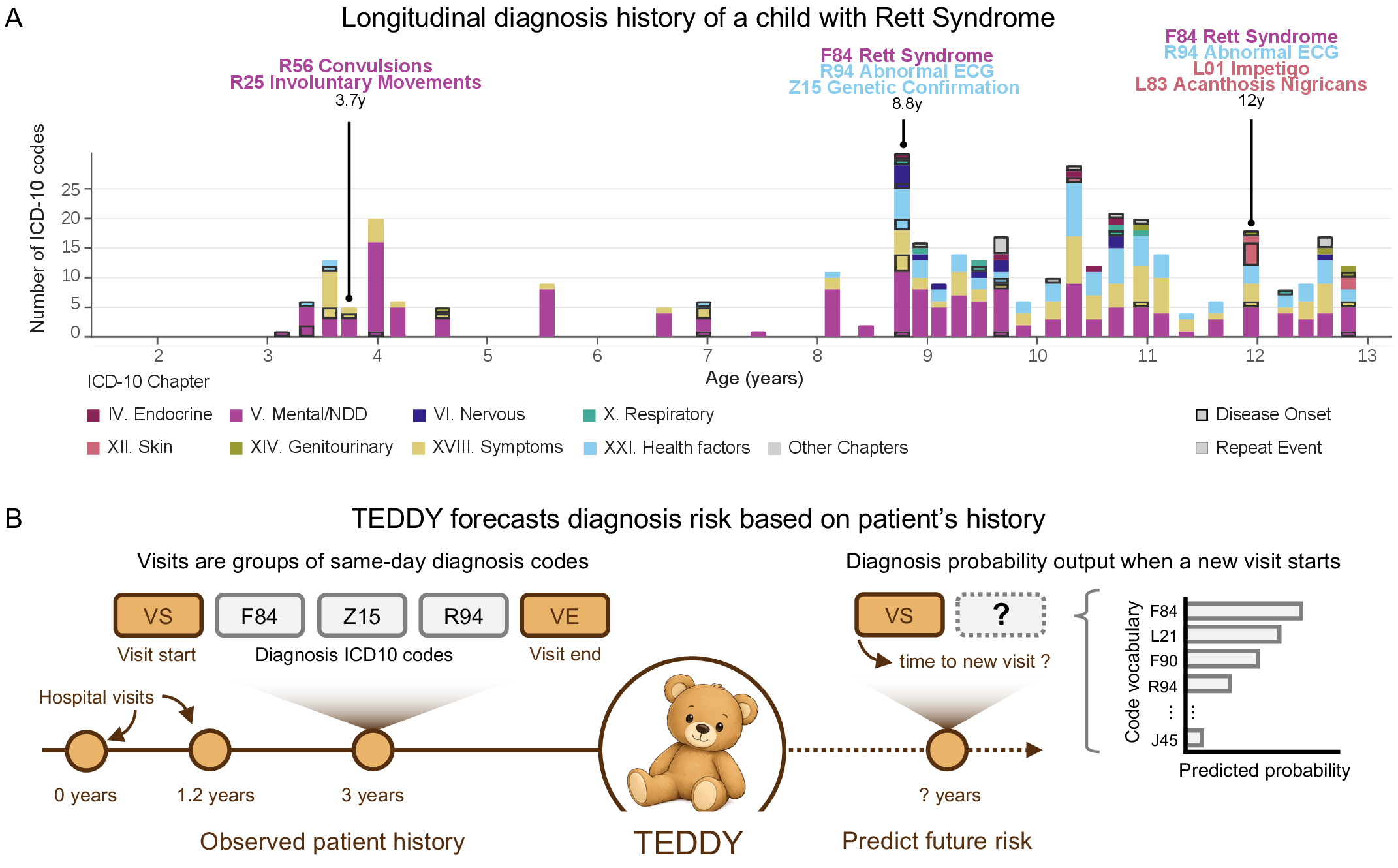
We score each condition only at its first appearance in a child’s record, never at later repeats: anticipating a genuinely new diagnosis is the task that matters clinically, whereas a condition a child already carries is easy to predict from its own past [20]. We ask TEDDY for its prediction at the start of a visit, before it can see any diagnosis entered that day, so it cannot quietly read codes that happen to share the same calendar day and inflate its own accuracy (Fig. 1; Methods). We compare each child who develops a condition only with children of the same sex and similar age, preventing the model from achieving high performance simply by recognizing that a condition occurs predominantly in boys, girls, newborns, or other age-defined groups. We report discrimination across the 16 ICD-10 chapters that capture intrinsic childhood disease, spanning infectious conditions through genitourinary disorders and including the perinatal and congenital chapters. Chapters recording administrative or non-diagnostic information — symptoms and abnormal findings, injuries and external causes, health-service factors, special-purpose codes, and pregnancy — are excluded. Unless we note otherwise, every AUC below is this same quantity: first appearance, sex- and age-matched controls, computed on diagnosis histories the model never saw during training.
TEDDY anticipates incident diagnoses across the range of childhood illness↩︎
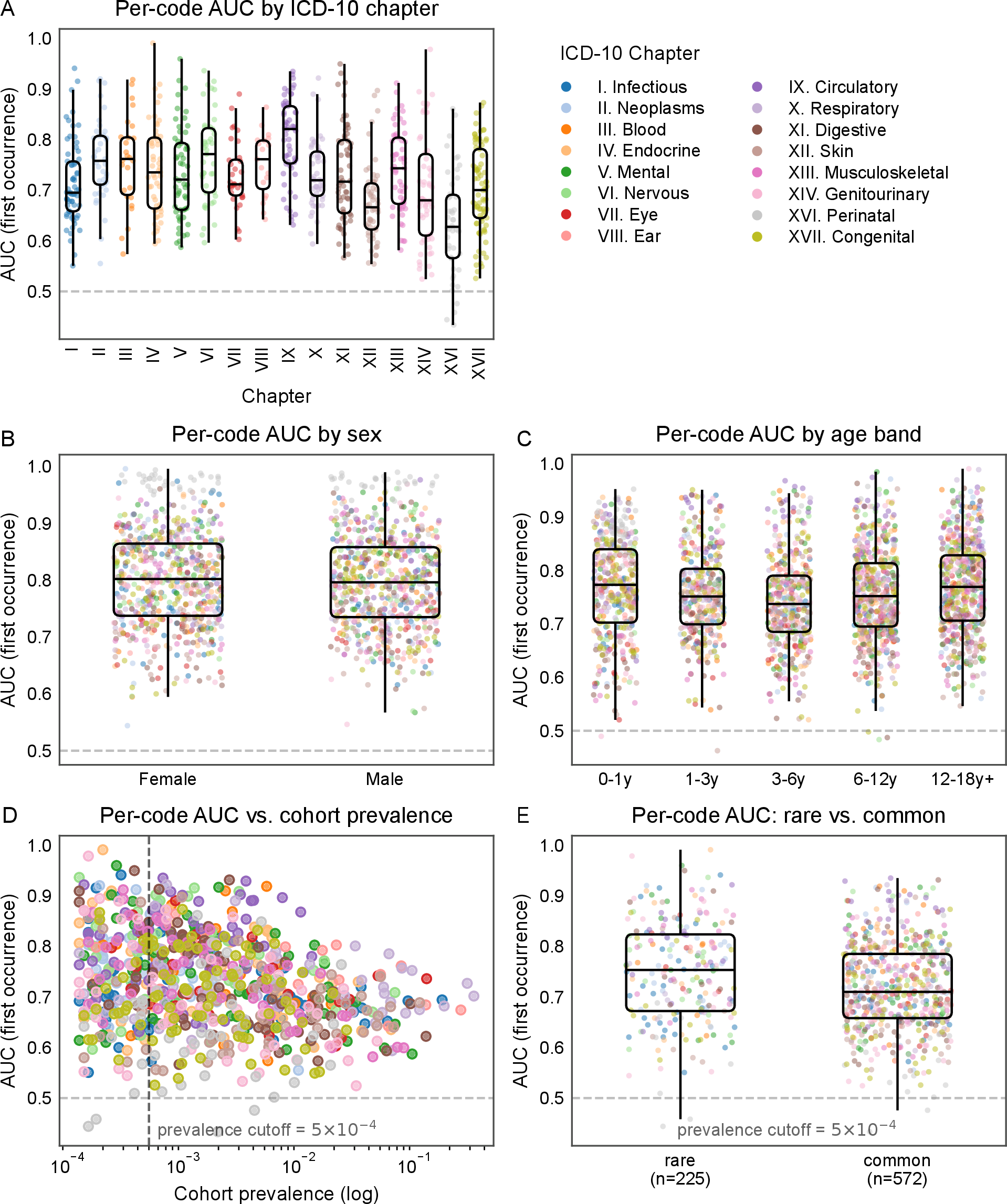
We first evaluated TEDDY across the full range of childhood illness, scoring every eligible condition rather than a hand-picked subset (Fig.2). Across 797 conditions spanning the 16 ICD-10 chapters of intrinsic childhood disease, the median first-occurrence AUC was 0.72, and the per-condition AUC distribution remained above chance within every chapter (Fig.2A).
TEDDY ranks risk similarly across sex and age. The distribution of per-condition AUCs is comparable for girls and boys (Fig.2B) and across the five pediatric age bands from infancy to late adolescence (Fig.2C). Because each child who develops a condition is compared only with controls of the same sex and similar age, this consistency across sex and age strata is not explained by demographic separability. Instead, it indicates that the model’s signal is broadly distributed across the pediatric population rather than concentrated in a demographically distinct subset of diagnoses.
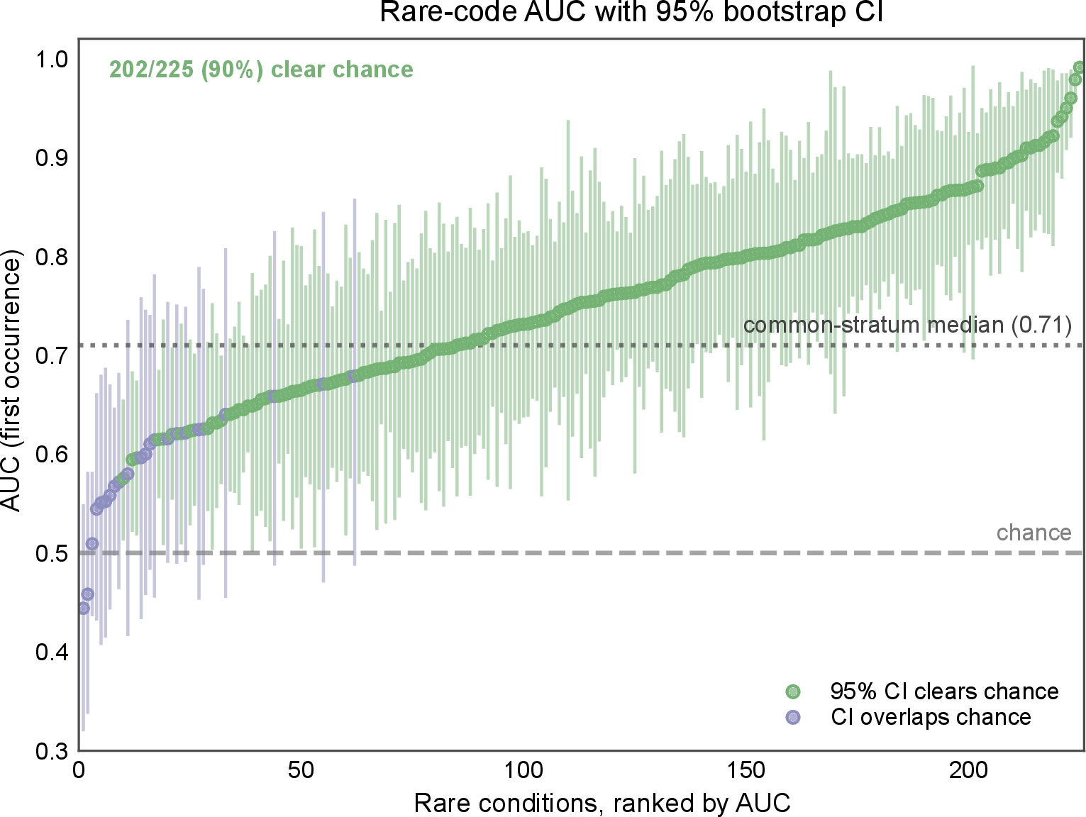
TEDDY performs particularly well where early recognition is often most difficult. Its per-condition AUC is higher among lower-prevalence diagnoses (Fig. 2D), and the 225 rarest conditions, each recorded in fewer than 5 of every 10,000 children, (\(5\times10^{-4}\)) — are anticipated at least as well as the 572 more common conditions (Fig.2E). A model that merely learned base rates would be expected to degrade on the long tail of rare disease; instead, TEDDY preserves discriminative signal for rare disease. This is not only wider estimation scatter at low prevalence: with patient-level bootstrap confidence intervals from 2,000 resamples, 202 of the 225 rarest conditions (90%) have a 95% CI lying entirely above chance (Supplementary Fig. 6). The rare-code discrimination is therefore a property of the model, not an artefact of estimating AUC from few cases.
TEDDY outperforms alternative architectures across diagnoses and in focused clinical benchmarks↩︎
Having established that TEDDY discriminates incident diagnoses across the pediatric disease spectrum, we next asked whether this performance could be recovered by alternative architectures trained on the same records. We compared TEDDY with DenseNet, convolutional neural network (CNN), recurrent neural network (RNN), and long short-term memory (LSTM) baselines across the same 797 first-occurrence diagnosis tasks. Each comparison was paired by ICD-10 code and used the same visit-boundary, first-occurrence evaluation framework.
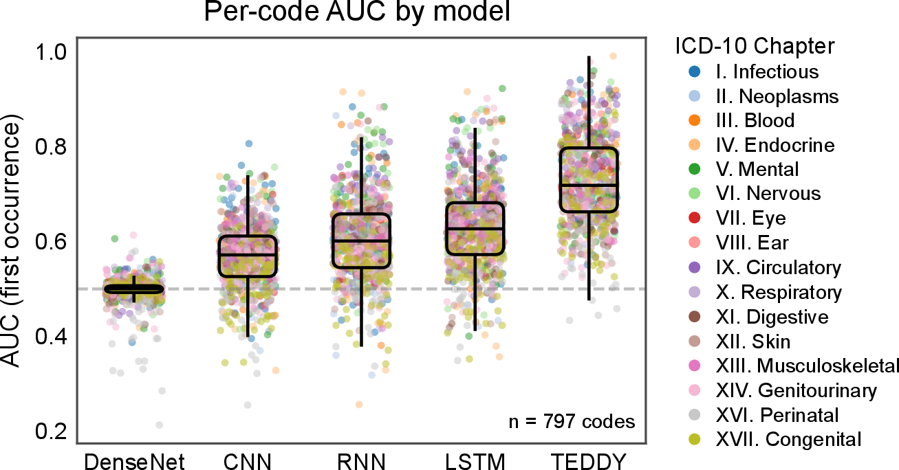
Across conditions, TEDDY showed a consistent upward shift in per-code AUC relative to every same-data baseline (Supplementary Fig. 7). The median first-occurrence AUCs for the baseline models ranged from 0.500 for DenseNet to 0.627 for LSTM, whereas TEDDY improved over each comparator on 96–99% of codes. The median paired improvement was largest against DenseNet (\(\Delta\)AUC = 0.224) and remained substantial against the strongest baseline, LSTM (\(\Delta\)AUC = 0.095). All four paired comparisons were significant after Holm correction (Supplementary Table 4). Thus, TEDDY’s advantage is not driven by a small number of favorable diagnoses and is not reproduced by simpler architectures trained on the same pediatric trajectories.
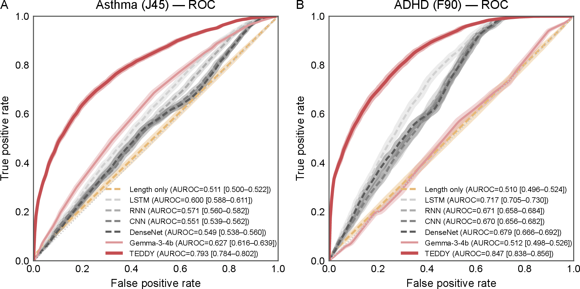
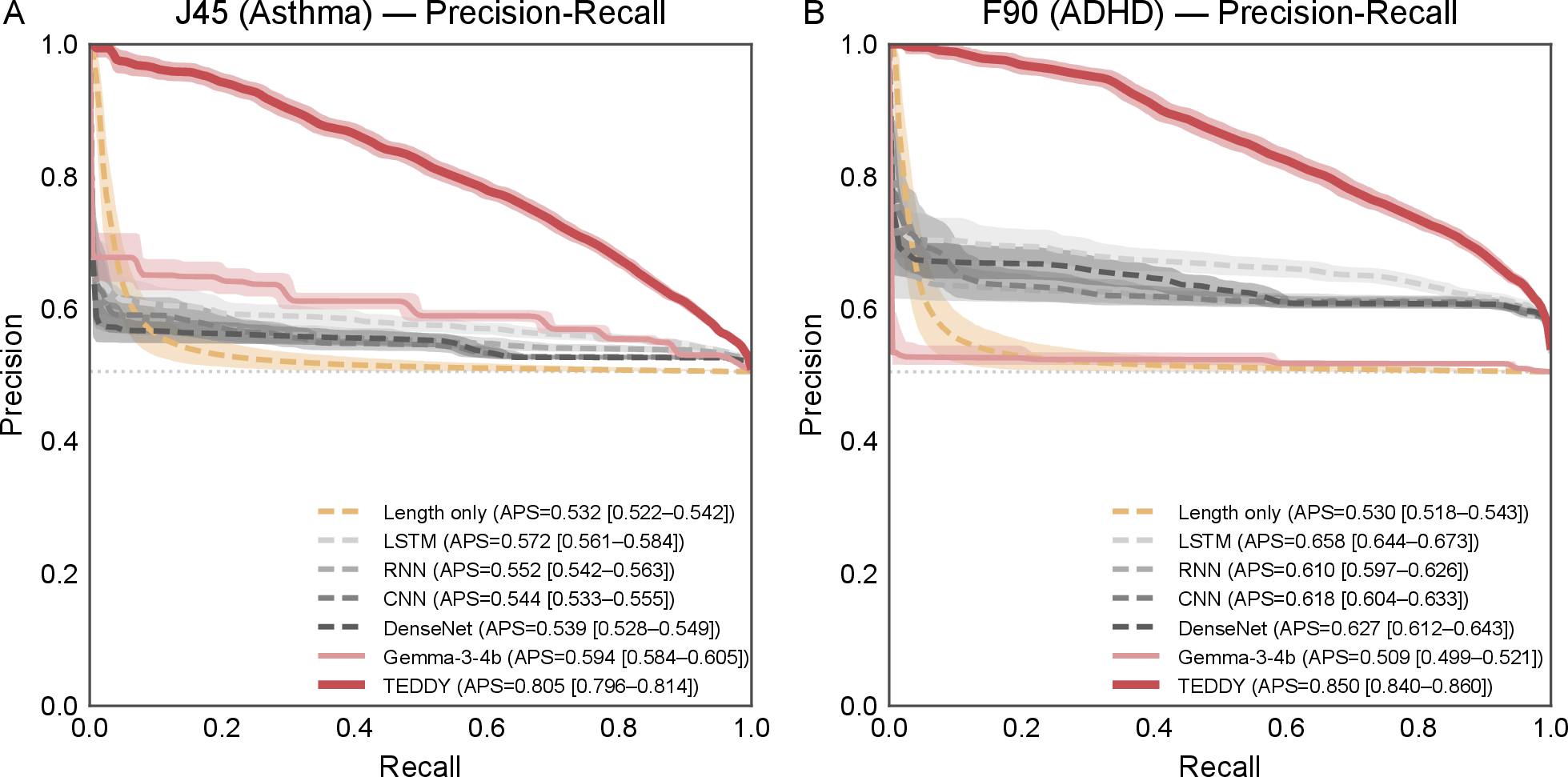
The broad per-code benchmark establishes the overall architecture-level advantage, but it does not show the full operating characteristics for individual clinically familiar outcomes. We therefore performed a focused head-to-head analysis of two common and clinically important pediatric diagnoses, asthma (J45) and attention-deficit/hyperactivity disorder (ADHD; F90). This analysis additionally included a history-length-only control and Gemma-3-4b, a general-purpose language model approximately three orders of magnitude larger, prompted on the same patient histories (Fig. 3).
TEDDY ranked risk most accurately for both targets, reaching an AUROC of 0.793 (95% CI 0.784–0.802) for asthma and 0.847 (0.838–0.856) for ADHD. It exceeded the strongest non-TEDDY comparator in each task with non-overlapping confidence intervals: Gemma-3-4b reached 0.627 (0.616–0.639) for asthma, while the strongest same-data sequence baseline for ADHD, the LSTM, reached 0.717 (0.705–0.730). Among the alternative architectures trained on the same dataset, the LSTM was also the strongest asthma baseline at 0.600 (0.588–0.611). Confidence intervals here and below are 95% patient-level bootstrap intervals from 2,000 resamples and are shown as shaded bands in Fig. 3 and Supplementary Fig. 8.
The focused comparison was designed to minimize the influence of trivial confounders. Every same-data sequence model saw the same children and records, while cases and controls were matched on history length so that no model could succeed merely by detecting that children with longer charts tend to be sicker. A predictor using history length alone remained near chance for both diagnoses (AUROC approximately 0.51). We also included Gemma-3-4b [33], a four-billion-parameter general-purpose language model prompted on the same histories. It performed above chance for asthma but near chance for ADHD, and remained well below TEDDY in both tasks. This comparison is best interpreted as a scale control rather than a direct test of parameter efficiency: a substantially larger general-purpose model without pediatric-trajectory training did not approach a smaller model developed specifically for longitudinal pediatric forecasting.
The same model ordering was observed under average precision, which measures enrichment of children who subsequently receive the target diagnosis (Supplementary Fig. 8). TEDDY reached 0.805 (95% CI 0.796–0.814) for asthma and 0.850 (0.840–0.860) for ADHD. For asthma, the strongest non-TEDDY comparator was Gemma-3-4b at 0.594 (0.584–0.605), and the strongest same-data sequence baseline was the LSTM at 0.572 (0.561–0.584). For ADHD, the strongest non-TEDDY comparator was the LSTM at 0.658 (0.644–0.673). Together, the broad per-code comparison and focused clinical benchmarks show that greater parameter count alone does not recover the performance of a model trained specifically on pediatric diagnosis trajectories.
TEDDY’s warning remains readable years in advance↩︎
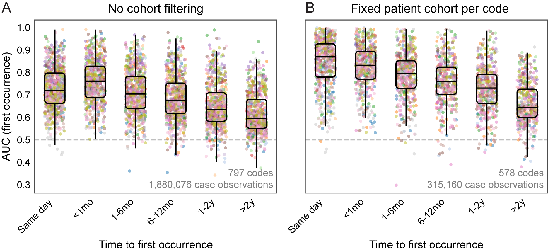
We define a warning as an interval before a condition’s first recorded diagnosis during which TEDDY’s risk estimate for that condition remains statistically discriminative between eventual cases and non-cases, a property of model output at a given lead time rather than a claim about a specific clinical alerting threshold. A warning is only useful if it arrives early enough to inform care. We therefore asked not only whether TEDDY can anticipate a new diagnosis, but how far before its first recorded occurrence that signal remains detectable. For each condition, we grouped scored visit-boundary positions by the time remaining until the target diagnosis first appeared, then computed a separate first-occurrence AUC within each lead-time band (Fig.4; Supplementary Table5).
In the unrestricted analysis, every eligible first-occurrence case contributes to its corresponding horizon band. Across 797 conditions and \(1{,}880{,}076\) first-occurrence case observations, discrimination declined gradually as the prediction horizon lengthened, but did not collapse to chance. The median per-code AUC was 0.718 on the same day (95% CI 0.711–0.730), increased to 0.761 within the month before the first diagnosis (0.750–0.771), and then decreased with longer lead times: 0.704 at 1–6 months (0.696–0.714), 0.675 at 6–12 months (0.667–0.684), 0.636 at 1–2 years (0.624–0.646), and 0.597 beyond two years (0.589–0.607). Thus, even when the diagnosis is still more than two years away, the median condition remains above chance (Fig. 4A).
Because the unrestricted analysis allows the contributing patients and codes to vary by horizon, we repeated the analysis using a stricter fixed patient cohort per code. In this sensitivity analysis, each code is evaluated only on patients who are available as first-occurrence cases in every active horizon band, so the decline is read on the same case set for that code across lead times. This fixed-cohort analysis retained 578 codes and \(315{,}160\) first-occurrence case observations. The same temporal pattern held, with higher absolute AUCs because the analysis is restricted to codes and patients evaluable across all horizons: median AUC declined from 0.869 on the same day (95% CI 0.856–0.880) to 0.832 at \(<\)1 month (0.821–0.843), 0.794 at 1–6 months (0.781–0.806), 0.760 at 6–12 months (0.750–0.771), 0.730 at 1–2 years (0.720–0.741), and 0.644 beyond two years (0.635–0.652) (Fig. 4B).
Together, these analyses show that TEDDY’s signal fades with distance from diagnosis but remains detectable years before the diagnosis appears in the chart. That persistence argues against the model that relies only on short-range links between neighboring visits. Instead, TEDDY captures longer trajectory structure that could support a forewarning role at routine pediatric visits, while making clear that discrimination is strongest close to the eventual diagnosis and weaker at multi-year horizons.
TEDDY estimates visit timing with small average error but long-tail drift↩︎
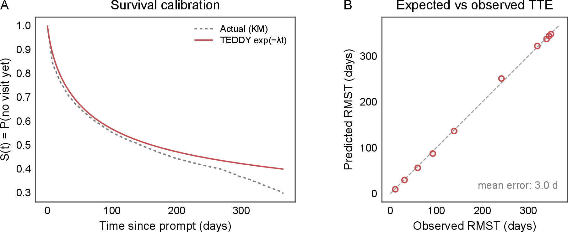
Beyond predicting a forthcoming diagnosis, TEDDY also estimates when a child will next be seen. We evaluated this estimate at the positions where the time-to-event head is trained to make it: visit boundaries and event-free intervals. This estimate is summarized as the restricted mean survival time (RMST), the expected time to the next event truncated at a fixed horizon. Across 200,000 sampled positions from the held-out test set, predicted and observed RMST were closely aligned across deciles of predicted return time, with a mean absolute RMST error of 3.0 days over a 365-day horizon (Fig. 5B).
The timing estimate also varies meaningfully across children rather than collapsing to a fixed follow-up interval. Among the \(94{,}799\) uncensored positions with an observed next visit, the model-implied and observed gaps were correlated after log transformation (Pearson \(r=0.54\) for \(\log(1+x)\)-transformed predicted and observed times; Spearman \(\rho=0.57\) on the raw times). This indicates that TEDDY has learned child-specific differences in return timing, not only the average visit cadence of the cohort.
The fit is not perfect, and we report where it falls short. Among observed return intervals, the observed median gap was 21.0 days, whereas the model-implied exponential median was 38.8 days. The predicted survival curve also drifts upward in the long tail: by one year, the observed probability of no return visit is 0.296, whereas the model predicts 0.399 (Fig. 5A). This limitation reflects the deliberately simple time head: a single exponential rate per position is easy to train and interpret, but too rigid to capture the full spread of real inter-visit intervals. Thus, TEDDY’s timing head is accurate on average and patient-specific, but should not be interpreted as a fully calibrated survival model.
Discussion↩︎
We set out to ask whether a generative model could anticipate incident diagnoses across the pediatric disease spectrum — a setting where the data come from one institution, where most possible diagnoses are individually rare even though most visits involve just a handful of common diagnoses, and where tools built for adults transfer poorly. The credibility of TEDDY’s numbers rests on the three guards built into its evaluation. Scoring each diagnosis the instant a visit begins, before that day’s codes are visible, prevents the within-encounter leakage a standard model would otherwise exploit. Scoring only first occurrences focuses the evaluation on the clinically important task of anticipating a newly recorded diagnosis – anticipating a new diagnosis — rather than re-predicting a condition a child already carries. And matching each case to controls of the same sex and similar age limits demographic composition from passing as clinical signal, a confound that inflates accuracy for any condition concentrated in one sex or age range. Each safeguard addresses a distinct route through which EHR forecasting performance can appear stronger. Together, they make TEDDY’s discrimination a more stringent estimate of predictive structure, rather than an artifact of same-visit information leakage, prior diagnosis documentation, or demographic imbalance.
Read that way, two features of the results carry clinical weight. TEDDY’s discrimination is broadly consistent across females and males and across the pediatric age range, indicating that its predictive signal is not confined to a demographically distinct subset of childhood illness. Moreover, contrary to the degradation often expected on long-tailed clinical data, median discrimination was highest among the rarest conditions rather than approaching chance as prevalence falls. This is particularly important in pediatrics: rare congenital and genetic disorders account for a substantial share of the diagnostic landscape and are among the conditions for which recognition is most often delayed [10]. That the signal remains detectable years before a diagnosis is recorded, rather than emerging only shortly before clinical recognition, motivates future evaluation of whether such signals could support risk review during routine pediatric encounters.
These results came from a model of only 1.84 million parameters trained on a single institution’s records. In the head-to-head view it outperformed four other sequence architectures trained on the same data and a general-purpose language model three orders of magnitude larger. The usual route to stronger EHR models has been ever-larger adult datasets and ever-larger models [19]–[21], a path largely closed to individual pediatric centers. Our results suggest that, in this setting, faithfully representing a child’s unfolding clinical trajectory may matter more than model size, which is encouraging for pediatric institutions that lack access to population-scale training corpora.
TEDDY’s sense of timing is calibrated where it is trained to be. Its predicted gap to the next visit tracked the observed gap with small average error, confirming that it learned child-specific visit rates rather than a single rate for everyone. The estimate over predicts the typical interval and departs from the observed long tail — the expected price of summarizing a skewed distribution of waiting times with a one-number rate — and we report this as a known limitation rather than smoothing over it.
Several limitations bound these conclusions. The records come from a single institution. Although TCH’s 1.6 million pediatric patients span a broad clinical population, coding practices, documentation patterns, and case mix vary across health systems, and we have not established whether TEDDY’s discrimination generalizes across those differences. The vocabulary is limited to ICD-10 diagnoses, so the model does not incorporate other structured EHR data, including vital signs, growth and BMI percentiles, laboratory values, imaging, procedures, or medications, which may provide additional predictive signal.
Three extensions follow naturally. The first is to widen the input beyond diagnoses, to measurements, medications, and procedures, and to test TEDDY across institutions and common data models. The second is intergenerational: the same model can be fine-tuned on mother-child pairs, with maternal prenatal history prepended to the child’s record, to ask whether maternal context gives calibrated predictive signal for the child. We have curated and held out a pretrain-disjoint dyad cohort for exactly this purpose. The third concerns recurrent critical events, such as repeated emergency presentations or relapses of an existing diagnosis, which we have not analyzed in depth here because a model can learn to anticipate a patient’s own recurring history rather than a risk pattern that generalizes, inflating apparent accuracy. Evaluation designs that separate first-occurrence prediction from recurrence prediction, or that limit the model’s access to a patient’s own prior instances of the same event, may reveal whether strong performance on recurrent events reflects genuine early signal or simple pattern repetition. A prospective, multi-site, multimodal pediatric trajectory model is the goal toward which this work is a first step.
Conclusion↩︎
TEDDY is a generative EHR foundation model built for children and evaluated under a leakage-free, demographically matched, first-occurrence protocol. On that footing, it anticipates incident diagnoses across the pediatric ICD-10 range — evenly across sex and age, most sharply for the rarest conditions, and years before they are recorded. At just 1.84 million parameters, it outperforms sequence baselines trained on the same data and a far larger language model. Extending the input across measurement channels and laboratory values, institutions, and mother–child trajectories is the path toward clinically actionable prediction.
Methods↩︎
Data and cohort↩︎
We assembled a single-site pediatric electronic health record corpus from Texas Children’s Hospital (TCH), comprising condition occurrences and patient demographics as of a 2026-01-22 data snapshot. We retained patients with at least three distinct ICD coded events and age \(\leq 25\) years, after within-encounter de-duplication (a diagnosis code recorded more than once for the same patient on the same calendar day is collapsed to a single event). Mother–infant dyads were identified using linkages recorded in the EHR, which associates each maternal delivery encounter with the corresponding newborn encounter at the time of birth. All dyad participants (mothers and infants; 81,847 patients) were excluded from the main pretraining corpus and held out as a patient-level disjoint cohort, so that any inter-generational transfer experiment on these dyads would be free of pretraining leakage (held as future work; see Discussion).
The final pretraining corpus contains 1,602,216 patients and \(\approx\)73 million ICD-10 condition events, drawn from a closed vocabulary of 1,849 tokens: 1,841 ICD-10-derived codes plus eight special tokens
(PADDING, BIRTH, NO_EVENT, SEX_FEMALE, SEX_MALE, SEX_UNKNOWN, VISIT_START, VISIT_END). ICD codes are truncated to chapter and subcategory (decimal
removed) prior to tokenization. At training time, to make prediction targets well-defined during long event-free intervals, we insert NO_EVENT tokens by gap-fill: between any two consecutive real events, a cursor advances forward by
an age-appropriate interval drawn from the American Academy of Pediatrics (AAP) well-child periodicity schedule [27] (Table 2), emitting a NO_EVENT token at each step until reaching the next real event. Real events are never displaced. Finally, we bracket each clinical visit: every maximal run of condition codes that a patient
receives on the same calendar day is wrapped between a VISIT_START and a VISIT_END token (both carrying that day’s age). Bracketing is applied after NO_EVENT gap-fill, so BIRTH and NO_EVENT
tokens remain between visits rather than inside them. We split patients 90/5/5 into train, validation, and test partitions and use the same patient-level split for every analysis in the paper unless explicitly noted.
| Age (days) | Age (clinical) | Interval (days) |
|---|---|---|
| \(\leq 30\) | \(\leq 1\) month | 15 |
| 31–365 | 1–12 months | 45 |
| 366–1,095 | 1–3 years | 135 |
| 1,096–4,380 | 3–12 years | 270 |
| 4,381–6,570 | 12–18 years | 365 |
| \(>6{,}570\) | \(>18\) years | 365 |
Every record is de-identified before modeling: a patient is represented solely by an integer study identifier, an ordered sequence of condition tokens, and, for each token, the patient’s age in whole days at the time of the event. Temporal information is stored exclusively as an age offset relative to birth (day \(0\)), so no calendar dates, admission or service times, ages in years, or other date-shiftable quantities are retained. The pipeline ingests only the patient identifier, the ICD-10 condition code, and this age-in-days offset; no names, medical record numbers, free-text notes, provider identifiers, or geographic fields are read at any stage. The data-snapshot date is used only to apply the age-eligibility cutoff and is not carried into the modeling corpus. Consequently the tokenized dataset consists entirely of surrogate identifiers, categorical condition codes, and integer day-offsets, and contains none of the protected health identifiers enumerated under the HIPAA Safe Harbor provision.
Tokenization and trajectory representation↩︎
Each patient is represented as a chronologically ordered sequence of (token, age) pairs drawn from the closed 1,849-token vocabulary described in the Data and cohort section, with ages stored as integer days from birth. The trajectory begins with a
synthetic BIRTH token at age 0, followed by the patient’s SEX_* token (also at age 0) and any condition codes recorded on the day of birth; subsequent condition codes appear in age order, and NO_EVENT tokens are
inserted between consecutive real events according to the AAP gap-fill cadence (Table 2). Consecutive condition codes recorded on the same day are then grouped into a visit: each such same-day run is delimited by
a VISIT_START and VISIT_END token pair, while BIRTH and NO_EVENT tokens pass through unbracketed between visits. Bracket tokens inherit the age of the visit they enclose.
Each patient is a single training example. We use a context window of 2,048 tokens; the bracketed trajectories have a median length of 59 tokens (p99 731), and the 0.23% of patients whose trajectory exceeds the context window are left-cropped to retain
only their most recent 2,048 tokens. Shorter sequences are right-padded with a dedicated PADDING token, and padded positions are ignored by both the loss and the attention mask. Events that share an integer age (i.e.same-day events) are
randomly reordered each epoch as a stochastic data-augmentation step; this does not change which tokens are visible at any prediction position.
Model architecture↩︎
Architecture. TEDDY is a decoder-only transformer (8 pre-norm layers, 8 attention heads, embedding dimension \(n_{\mathrm{embd}}=128\); [34], [35]) with weight-tied input and output embeddings, yielding \(1{,}839{,}488\) trainable parameters (\(\approx\)1.84M). Each input position carries two embeddings that are summed before the first transformer block: a learned token embedding \(\mathbf{e}_{\mathrm{tok}}(x_t) \in \mathbb{R}^{128}\) indexed by the token id \(x_t \in \{0, \ldots, 1{,}848\}\), and an age encoding \(\mathbf{e}_{\mathrm{age}}(a_t) \in \mathbb{R}^{128}\) that maps the patient’s age in days \(a_t\) to a sinusoidal feature vector (period bank with maximum wavelength \(10^{4}\), applied to age in years \(a_t/365.25\)) followed by a bias-free linear projection. We use no learned positional embeddings: temporal ordering enters the model exclusively through this age channel and through a standard triangular (causal) attention mask, under which position \(t\) attends to all positions \(s \leq t\). Each transformer block consists of LayerNorm, multi-head causal self-attention, residual connection, LayerNorm, and a GELU MLP with 4\(\times\) expansion. We use dropout \(p=0.1\) throughout and a final LayerNorm before the output projection.
Output and loss. Our training objective builds on the Delphi-2M framework for joint token-and-time modeling of disease trajectories [19], which our work extends in several directions described in the following sections. A single linear head (weight-tied to the input embedding) projects the final hidden state
at position \(t\) to logits \(\mathbf{z}_t \in \mathbb{R}^{1849}\). These logits parameterise two things simultaneously: (i) the next-token distribution, used in the categorical
cross-entropy loss \(\mathcal{L}_{\mathrm{CE}}\) over the predicted token; and (ii) the rate \(\lambda_t = \exp(\mathrm{logsumexp}(\mathbf{z}_t))\) of an exponential
time-to-next-visit distribution, used in a negative log-likelihood loss \(\mathcal{L}_{\Delta t}\) over the interval \(\Delta t_t = a_{t+1} - a_t\) to the next visit boundary.
Because visits are explicitly bracketed (the Tokenization and trajectory representation section), the model predicts elapsed time only at positions whose target begins a new visit or a NO_EVENT interval — that is, the time clock advances per
visit transition rather than at every within-visit code — whereas the categorical loss applies at every predictable position.
The NO_EVENT tokens are inserted on a fixed well-child cadence rather than observed at true encounters, so they mark points at which a visit had not yet occurred: right-censored observations of the latent time-to-next-visit rather
than events. We therefore treat every NO_EVENT target as right-censored in the time loss. Such positions contribute the survival term \(-\log S(\Delta t_t) = \lambda_t\,\Delta t_t\) rather than the full event
density \(-\log f(\Delta t_t) = -\log\lambda_t + \lambda_t\,\Delta t_t\), while positions whose target is a genuine visit boundary contribute the event density as usual. This censoring applies only to the time loss;
NO_EVENT remains an ordinary categorical target in \(\mathcal{L}_{\mathrm{CE}}\). Because NO_EVENT accounts for roughly half of inter-visit positions (up to \(\sim\)80% in infancy), charging the full event density at these positions otherwise biases the learned rate toward the synthetic cadence grid. We train against the convex combination \(\mathcal{L} =
\mathcal{L}_{\mathrm{CE}} + \mathcal{L}_{\Delta t}\). Context-only tokens (PADDING, BIRTH, SEX_*) are excluded from the prediction targets and the loss; NO_EVENT, the visit-bracket tokens
(VISIT_START, VISIT_END), and ICD codes are all predictable.
Training↩︎
We optimise the composite loss \(\mathcal{L} = \mathcal{L}_{\mathrm{CE}} + \mathcal{L}_{\Delta t}\) with AdamW [36] and a cosine learning-rate schedule peaking at \(6\times 10^{-4}\) after a linear warmup over the first 10% of training iterations, for five epochs. We train in bfloat16. Padded
positions and context-only tokens (PADDING, BIRTH, SEX_*) are masked from attention and excluded from prediction targets; NO_EVENT and the visit-bracket tokens remain predictable under \(\mathcal{L}_{\mathrm{CE}}\), while NO_EVENT targets are treated as right-censored in the time loss \(\mathcal{L}_{\Delta t}\). The headline model was trained data-parallel across
eight NVIDIA A100 GPUs, giving an effective batch of 32 sequences per optimizer step.
Per-code AUC: estimation and demographic matching↩︎
For each of the \(1{,}841\) ICD codes \(c\) (of the \(1{,}849\)-token vocabulary), we estimate a per-code AUC with the Mann–Whitney \(U\) statistic comparing the model’s logit for \(c\) between cases and controls. The logit is always read at a VISIT_START position — the model’s estimate, on entering a visit, of
the codes that visit will contain. Reading the score there, rather than from a neighbouring same-day code, is what makes the estimate leakage-free (the Tokenization and trajectory representation section): because the codes recorded on a single calendar day
carry no inherent order, scoring at VISIT_START takes the prediction before any of that day’s codes have been supplied as input. A case for \(c\) is a VISIT_START opening a visit in which
\(c\) is recorded; a control is a VISIT_START from a patient who never has code \(c\) recorded anywhere in their trajectory. Each patient contributes a single such
position to the estimate. Codes with fewer than 20 cases or 20 controls are excluded — the case threshold is set low to retain rarer codes. We retain sixteen ICD-10 chapters that capture intrinsic childhood disease and exclude chapters that record
administrative or non-diagnostic information: symptoms and abnormal findings (R); injuries and external causes (S–T, V–Y); factors influencing health status and contact with services (Z); special-purpose codes (U); and pregnancy, childbirth, and the puerperium (O). The codes that pass the case threshold within these chapters are the conditions scored throughout (Results). We report first-occurrence AUC (the case restricted to the first visit in which \(c\)
appears), with a 95% confidence interval.
The discrimination confidence intervals for both the per-code AUCs here (Fig. 2, Supplementary Fig. 6) and the head-to-head AUROC and average-precision intervals of the model benchmark (Fig. 3, Supplementary Fig. 8) are computed by the same patient-level nonparametric bootstrap: the units being scored are resampled with replacement \(2{,}000\) times, the same estimator is recomputed on each replicate, and the \(2.5\)th and \(97.5\)th percentiles of the resulting distribution are taken as the interval. The two analyses differ only in what one unit is and which estimator is recomputed. For the per-code AUC, each patient contributes a single scored position, so resampling the case and control rows is equivalent to resampling patients, and each replicate recomputes the sex- and age-matched weighted Mann–Whitney AUC defined below; for the benchmark, the unit is a cohort patient’s \((\text{label},\text{score})\) pair and each replicate recomputes the unweighted AUROC and average precision (and, for the curve bands, the ROC and precision–recall curves interpolated onto a common grid). Resampling the matched estimator itself, rather than using the analytic DeLong variance for the unweighted statistic, propagates the uncertainty of the demographic reweighting into the per-code intervals; in both analyses the bootstrap centre reproduces the reported point estimate (to within \(10^{-4}\) for every per-code AUC), so each interval is anchored to the value it accompanies. The future-horizon median confidence intervals (§6; Supplementary Table 5) use a different unit and are not part of this patient-level procedure: because the reported quantity is the median AUC across conditions within a horizon band, each interval is a condition-level bootstrap, resampling the set of per-code AUC values with replacement \(2{,}000\) times and taking the \(2.5\)th and \(97.5\)th percentiles of the resulting medians.
We examine the per-code intervals in particular for the rare stratum, to separate genuine rare-code signal from the wider estimation scatter expected at low prevalence: \(202\) of the \(225\) rarest conditions (\(90\%\)) have a first-occurrence interval lying entirely above chance (Supplementary Fig. 6).
To ensure that cases and controls are demographically comparable in the pooled estimate, we reweight controls to match the joint sex and age-band distribution of the cases for each code. Sex is encoded as female, male, or unknown (unknowns are matched only to unknowns). Each control receives a non-negative weight \(w = (n^{\mathrm{case}}_{sb} / n^{\mathrm{case}}) / n^{\mathrm{ctrl}}_{sb}\) within its (sex, band) cell \(sb\); strata in which cases exist but no control is available are dropped and their case mass reported as a coverage deficit. Age bands follow a coarsen-then-fall-back cascade: we begin with a fine 15-band pediatric schema (0–1mo, 1–3mo, 3–6mo, 6–12mo, 1–1.5y, 1.5–2y, 2–3y, 3–4y, 4–6y, 6–8y, 8–10y, 10–12y, 12–15y, 15–18y, 18y+) and, whenever case-coverage falls below 0.5, fall back first to the 5-band AAP scheme (0–1y, 1–3y, 3–6y, 6–12y, 12–18y+), then to a 3-band coarse scheme (0–3y, 3–12y, 12–18y+), and finally to sex-only matching. For each code we report the Kish effective sample size \(n_{\mathrm{eff}} = (\sum_i w_i)^2 / \sum_i w_i^2\), which equals the control count under uniform weights and shrinks as weight mass concentrates.
Future-horizon discrimination↩︎
A central question for a trajectory model is not merely what a patient’s next visit will contain, but how far into the future a diagnosis can be anticipated. We measure this with a future-horizon analysis: at each scored
VISIT_START position, we record the horizon from that visit boundary to the nearest future occurrence of the target code anywhere in the remainder of that patient’s trajectory. Scored positions are then assigned to one of six
lead-time bands: Same day, <1mo, 1–6mo, 6–12mo, 1–2y, and >2y (Table 3). For each ICD-10 code and each horizon band, we compute a first-occurrence AUC comparing
cases whose next occurrence of the target code falls in that band against matched controls who never receive the target code. This analysis measures how rapidly diagnostic discrimination decays as the forecasting window lengthens.
Each per-code, per-horizon AUC reuses the case/control estimator and the sex \(\times\) age matching cascade described above. Controls are drawn from patients who do not carry the target code anywhere in their full
trajectory, and are reweighted to match the sex and age distribution of cases within each code–horizon stratum. We require at least 100 total future cases per code, at least five cases in a code–horizon cell, at least 20 eligible controls, and a minimum
matching coverage of 0.5. The unit of analysis is the scored position, not the patient: for each code, every eligible pre-diagnosis VISIT_START position contributes a separate case to the horizon band matching its own distance to that code’s
nearest future occurrence, so a single patient may contribute multiple case observations to the same code — even within a single horizon band, if several of their visits precede the same eventual diagnosis at similar lags — and the patients and codes
contributing to the estimate may vary across lead times.
To test whether the temporal decline is driven by changing cohort composition rather than loss of predictive signal, we also run a fixed-cohort sensitivity analysis. For each code, we restrict to patients who are evaluable as first-occurrence cases in every active horizon band for that code, and then compute the same matched per-code AUC separately within each band. Thus, within a code, the same case set is followed across lead times. This fixed-cohort analysis is more stringent and retains fewer codes and observations, but it makes the horizon trend less sensitive to differences in which patients contribute to each bin.
For both the unrestricted and fixed-cohort analyses, the figure reports the distribution of per-code AUCs across conditions within each horizon band. Supplementary Table 5 reports the median per-code AUC and a 95% bootstrap confidence interval for that median, computed with 2,000 condition-level resamples.
| Bin | Lead time to first occurrence |
|---|---|
| Same day | 0 days |
| \(<\)1mo | \(>0\) to \(<30\) days |
| 1–6mo | 30 to \(<180\) days |
| 6–12mo | 180 to \(<365\) days |
| 1–2y | 365 to \(<730\) days |
| \(>\)2y | \(\geq 730\) days |
Stratified AUC: sex, age, and prevalence↩︎
Beyond the pooled per-code AUC, we report three stratified views that surface where discrimination varies across the cohort. Each view applies the same Mann–Whitney estimator and one-position-per-patient control sampling as in the Per-code AUC section, computed independently within each stratum, so the stratified AUCs are directly comparable to the pooled column. First, we stratify by sex, computing per-code AUC separately within the female and male strata (positions of unknown sex are excluded). Second, we stratify by age using the 5-band AAP scheme (0–1y, 1–3y, 3–6y, 6–12y, 12–18y+), with positions outside all bands excluded; this reveals how a code’s predictability shifts across the pediatric age range. Third, we stratify by prevalence, splitting the vocabulary into rare and common codes at a single participant-prevalence threshold (a code is rare if fewer than five in ten thousand patients ever receive it) and comparing the AUC distributions of the two strata, which quantifies how much of the model’s discrimination is carried by common versus long-tail codes.
Temporal calibration of time-to-next-visit↩︎
Because TEDDY supervises elapsed time only at visit boundaries and NO_EVENT checkpoints (§3), we assess the calibration of its predicted time-to-next-visit at exactly those positions. We draw a sample of \(200{,}000\) scored positions from the held-out test split whose target is VISIT_START (an observed visit) or NO_EVENT (a right-censored inter-visit checkpoint), and at each, convert the time head’s
predicted rate \(\lambda_t\) into a survival function \(S(t)=\exp(-\lambda_t t)\), the model’s probability that no further visit has occurred by elapsed time \(t\). We compare the population-averaged model survival curve against the empirical Kaplan–Meier estimate over the observed inter-visit intervals, treating VISIT_START as an event and NO_EVENT as
censoring. To summarise agreement on the restricted-mean-survival-time (RMST) scale, we group the sampled positions into ten deciles of predicted RMST (area under the model’s survival curve out to a 365-day horizon), and within each decile compare the mean
predicted RMST against the observed RMST (the area under the decile’s KM curve). The reported mean absolute RMST error is the sample-size-weighted average of this predicted-vs-observed gap across the ten deciles, not an average over individual positions.
Because the head emits a single exponential rate per position, this evaluation probes whether that rate is context-dependent and well-scaled rather than whether the inter-visit distribution is itself exponential; any divergence of the fitted exponential
from the Kaplan–Meier tail therefore reflects the deliberate simplicity of the per-position model rather than a miscalibration of its central tendency.
Baselines↩︎
We compare TEDDY against two baselines, each calibrated to a different counterfactual.
Alternative sequence architectures. To isolate the effect of the transformer architecture from the effect of training a generative model on EHR sequences, we train four alternative architectures — a two-layer LSTM, a two-layer vanilla RNN, a two-layer CNN (kernel size 3), and a two-layer DenseNet — on the same canonical dataset, with matching embedding dimension (\(n_{\mathrm{embd}}=128\)), context window (2,048 tokens), optimiser, learning-rate schedule, and mixed-precision settings. These baselines are size-matched to TEDDY in width and training recipe and are no larger in parameter count, so the only model in our comparison that exceeds TEDDY’s scale is the general-purpose Gemma-3-4b introduced below. All four are evaluated through the same per-code AUC pipeline as TEDDY.
General-purpose LLM head-to-head. As an external comparator we benchmark google/gemma-3-4b-it, a 4-billion-parameter instruction-tuned LLM accessed via Amazon Bedrock, on a binary next-ICD-code task framed identically for
both models so the results are directly comparable. For a chosen target code (J45 / asthma is the default headline; the cohort builder accepts any 3-character ICD-10 code), we draw the case/control cohort from the same test split as TEDDY‘s evaluation. Cases are patients with at least one recorded occurrence of the target code; the prediction cutoff is set at the first occurrence, with at least five real ICD events required in the preceding history. Controls
are patients with no occurrences of the target and at least one ICD event after a sampled cutoff; the cutoff position is drawn from the cases’ empirical history-length CDF (seed 42) so length cannot trivially separate the two groups. We optionally enforce
strict length matching (Kolmogorov-Smirnov \(\approx 0\)) as a sensitivity check.
Each patient’s pre-cutoff history is rendered as a single text prompt under one of four variants that vary along two orthogonal axes — representation (raw ICD codes vs.ICD-10 subblock terms) and ordering (top-frequency unordered vs.chronological with
age annotations) — giving codes_only, code_at_age, terms_only, and terms_at_age. The model is asked to return a single floating-point risk score, which is parsed by regex from the response. We use
temperature \(=0\), max-new-tokens 64, 4-way thread parallelism, and exponential-backoff retries on transient Bedrock errors (up to 5 attempts).
To put TEDDY on the same scoring axis we exploit the competing-exponentials structure of its head: under that parametrisation, \(\mathrm{softmax}(\mathbf{z}_t)_c\) at the last valid position is exactly the probability that the next event is code \(c\). We slice each cohort patient’s trajectory to the same cutoff, run a single forward pass through the canonical TEDDY checkpoint, and read out \(P(\text{next}=\text{target})\) directly from the output softmax. Both models are scored on AUROC and average precision over the same cohort, so any performance difference between Gemma and TEDDY can be attributed to the modelling and not to differences in cohort construction or scoring axis.
Reproducibility and artifacts↩︎
The patient-level electronic health record data underlying this study contain protected health information and cannot be shared: neither the raw records nor the de-identified tokenized corpus, trained model checkpoints, or per-position evaluation caches are publicly released, as each is derived from protected patient data and is subject to the institutional review board approval and data-use agreements governing the TCH EHR. Access to derived artifacts may be considered on reasonable request to the corresponding authors, subject to institutional approval and an appropriate data-use agreement. The implementation, configuration files, and analysis scripts that produce every result in this paper are open source at https://github.com/LiuzLab/teddy, so the full pipeline can be reproduced against an equivalently formatted cohort.
Ethics Approval↩︎
This study was conducted in accordance with the Declaration of Helsinki and approved by the Baylor College of Medicine Institutional Review Board (protocol code H-52222; date of approval 2 October 2025). The requirement for informed consent and HIPAA authorization was waived because the study involved retrospective analysis of existing clinical data, posed no greater than minimal risk to participants, and obtaining individual consent was impracticable.
Supplementary Figures and Tables↩︎
| Comparator | Median AUC | Median \(\Delta\)AUC | Codes favoring TEDDY | Adjusted \(P\) |
|---|---|---|---|---|
| DenseNet | 0.500 | 0.224 | 792/797 (99%) | \(3.9\times10^{-131}\) |
| CNN | 0.572 | 0.158 | 784/797 (98%) | \(5.0\times10^{-130}\) |
| RNN | 0.601 | 0.117 | 775/797 (97%) | \(1.7\times10^{-129}\) |
| LSTM | 0.627 | 0.095 | 769/797 (96%) | \(5.0\times10^{-126}\) |
| A. No cohort filtering | B. Fixed cohort | |||||||||
|---|---|---|---|---|---|---|---|---|---|---|
| 2-6(lr)7-11 Horizon | Median | 95% CI | \(n_{\text{codes}}\) | \(n_{\text{patients}}\) | \(n_{\text{obs}}\) | Median | 95% CI | \(n_{\text{codes}}\) | \(n_{\text{patients}}\) | \(n_{\text{obs}}\) |
| Same day | 0.718 | [0.711, 0.730] | 797 | 74,452 | 556,972 | 0.869 | [0.856, 0.880] | 578 | 14,515 | 54,254 |
| \(<\)1 mo | 0.761 | [0.750, 0.771] | 675 | 41,956 | 205,217 | 0.832 | [0.821, 0.843] | 475 | 13,948 | 52,787 |
| 1–6 mo | 0.704 | [0.696, 0.714] | 675 | 48,597 | 336,607 | 0.794 | [0.781, 0.806] | 461 | 13,757 | 52,409 |
| 6–12 mo | 0.675 | [0.667, 0.684] | 623 | 43,426 | 287,635 | 0.760 | [0.750, 0.771] | 436 | 13,372 | 51,892 |
| 1–2 y | 0.636 | [0.624, 0.646] | 618 | 42,395 | 270,013 | 0.730 | [0.720, 0.741] | 438 | 13,336 | 51,915 |
| \(>\)2 y | 0.597 | [0.589, 0.607] | 608 | 39,875 | 223,632 | 0.644 | [0.635, 0.652] | 437 | 13,324 | 51,903 |