Closed-Loop Knowledge Dynamics: An Operational Framework for Saturation and Escape
July 15, 2026
Abstract
Feedback-driven loops support iterative improvement in large language models, reinforcement learning, and autonomous discovery, yet their gains often diminish under repeated internal feedback. We study why closed-loop knowledge systems saturate and what external information can move them beyond their current attractors. We introduce a three-level operational framework in which knowledge states \(x_t\) evolve through transition kernels \(K_{\theta}\) indexed by a structural parameter \(\theta\). The governing structure is defined as the observational equivalence class of \(\theta\) induced by these kernels, while attractors and basins are properties of the fixed-\(\theta\) dynamics. A structural intervention changes \(\theta\) and produces a detectable kernel discrepancy on pre-specified probe states, making structural change falsifiable. Using a Lyapunov drift condition, we show that stable internal dynamics approach bounded stability regions with exponentially attenuated transients and a noise-controlled residual floor. We characterize escape through a metric condition on intervention-induced attractor displacement and a baseline-relative KL lower bound for increasing escape probability. This analysis also explains why conditional mutual information alone cannot certify escape: it measures variation among intervention-conditioned updates rather than departure from the no-intervention law. Case studies in LLM code repair, sparse-reward reinforcement learning, and Bayesian optimization use matched continuation controls to illustrate how feedback strength and alignment affect quality-improving escape. Our contribution is an operational connection among stability tools, measurable intervention effects, and cross-domain diagnostics.
1 Introduction↩︎
Modern AI systems increasingly rely on closed feedback loops. Large language models (LLMs) refine their outputs through self-reflection and revision, reinforcement learning (RL) algorithms update policies from environmental rewards, and autonomous discovery systems revise hypotheses based on experimental evidence. Despite their different forms, these systems share a common structure: a knowledge representation produces an output, receives feedback, and updates itself repeatedly.
A striking empirical pattern appears across such systems. Improvement is often rapid in early iterations, but marginal gains gradually diminish as the loop is repeated. LLM self-refinement improves drafts for several rounds and then stabilizes; RL policies approach stable value or policy regions; and belief-guided discovery systems increasingly concentrate their search as uncertainty is resolved. This suggests that saturation may not be merely an artifact of a particular algorithm, prompt, or benchmark, but a broader phenomenon of feedback-driven knowledge evolution.
This raises a basic question: what governs the long-term dynamics of closed-loop knowledge systems, and under what conditions can a saturated system move beyond its current attractor? Existing theories provide partial answers within individual domains. Contraction mappings explain the convergence of Bellman operators in RL; Bayesian optimization analyzes uncertainty-guided exploration; dynamical systems theory provides tools for stability and attractors; and information theory quantifies the value of new observations. These theories provide the relevant mathematical ingredients, but they do not by themselves supply a shared experimental interface for distinguishing three different observations: movement of the current state, a persistent change in the update law, and quality-improving escape from a pre-specified basin.
We develop an operational framework for closed-loop knowledge dynamics. The framework separates three levels: observable knowledge representations \(x_t\), transition kernels \(K_{\theta}\), and an explicit structural parameter \(\theta\). A fixed \(\theta\) induces the internal-loop kernel whose attractors and basins are then derived. Structural change is defined as an update of \(\theta\) that produces a detectable kernel discrepancy on pre-specified probes; a one-off state change without such a discrepancy is not labeled structural.
The resulting picture is a saturation–escape principle. Stable internal feedback drives knowledge representations toward epistemic attractors, where marginal improvement becomes increasingly limited. Escaping such regimes requires more than additional internal iteration: it requires external input that changes the probability of leaving the old basin. We characterize this through a metric sufficient condition for attractor relocation and a baseline-relative information-divergence requirement for increasing escape probability.
Our contributions are as follows:
We formulate closed-loop knowledge dynamics as a three-level operational model separating observable representations, transition kernels, and an explicit structural parameter. We define structural change through a pre-specified kernel discrepancy, making the governing structure identifiable up to observational equivalence and empirically falsifiable.
We turn classical Lyapunov drift and contraction-plus-noise conditions into cross-system saturation diagnostics, including an exponential-plus-floor signature and explicit residual stability regions.
We derive quantitative escape conditions for saturated systems. A metric condition relates parameter-induced attractor relocation to one-step escape, while a baseline-relative KL bound gives a necessary information-divergence budget for increasing escape probability. We explicitly separate this quantity from conditional mutual information.
We evaluate the resulting diagnostics in LLM code repair, sparse-reward reinforcement learning, and Bayesian optimization using controls that separate additional internal iteration from the effect of external feedback.
The mathematical ingredients are deliberately classical. The methodological contribution is their coupling into falsifiable hypotheses with matched baseline distributions, pre-specified escape events, and explicit tests for structural change. This positioning allows the framework to be evaluated by whether it improves measurement and intervention design across systems, rather than by whether it introduces a new Lyapunov or information inequality.
2 Related Work↩︎
2.0.0.1 Dynamical-systems views of learning.
Dynamical-systems tools provide a natural language for analyzing iterative learning processes. Robbins–Monro stochastic approximation and its ODE method [1]–[3] study convergence toward roots of expected vector fields, while Foster–Lyapunov drift criteria characterize stochastic stability through one-step contraction inequalities [4]. Contraction mappings also underlie classical RL guarantees, such as the \(\gamma\)-contraction of the discounted Bellman operator [5]. These theories provide powerful tools for analyzing a fixed transition rule, but they typically do not distinguish the observable knowledge representation, the transition operator, and the higher-level structure that determines which attractors and basins the operator induces.
2.0.0.2 Recursive self-refinement and saturation.
LLM self-refinement methods such as Self-Refine [6] and Reflexion [7] show that repeated critique and revision can improve model outputs over multiple rounds. Fixed-point iteration is often invoked informally to explain eventual stabilization, and recent work reports convergence-like behavior in latent concepts and uncertainty during self-correction [8]. However, these works do not provide a common operational test that separates trajectory stabilization, structural change, and quality-improving escape. We complement this literature by connecting an exponential-plus-floor diagnostic under contraction-plus-noise to a metric relocation condition and a baseline-relative information-divergence threshold.
2.0.0.3 Closed-loop discovery, effective landscapes, and external information.
Bayesian optimization and bandit methods study how evidence guides search under uncertainty; GP-UCB balances posterior mean estimates with uncertainty bonuses [9]. Recent closed-loop discovery frameworks, such as GAMBLe, analyze generator–assessor–search systems and the effective landscapes they induce [10], while work on self-evolving language models studies when internal self-play plateaus without learnable information gain [11]. LLM-guided and multi-fidelity Bayesian optimization methods such as LABO and LGBO further examine when auxiliary or low-cost LLM signals accelerate search and when they should be gated or incorporated conservatively [12], [13]. These works are closely related to our view that external information helps only when it is sufficiently reliable and informative, but our focus is on general saturation and escape conditions for closed-loop knowledge dynamics rather than a specific search-system decomposition or acquisition rule.
3 Mathematical Framework↩︎
3.1 Closed-Loop Knowledge Dynamics↩︎
We formalize closed-loop AI systems as processes in which a knowledge representation repeatedly produces an output, receives feedback, and updates itself. The central object is not a particular algorithm, but the evolution of knowledge representations under feedback.
Let \(\mathcal{X}\) denote a knowledge representation space. An element \(x_t\in\mathcal{X}\) may represent a draft, answer, policy, hypothesis, belief state, or other internal representation of knowledge. A closed-loop knowledge system consists of an output operator, a feedback operator, and an update operator: \[\mathcal{K} = (\mathcal{X},\mathcal{Y},\mathcal{E},\Omega,G,H,\Phi),\] where \(\mathcal{Y}\) is the output space, \(\mathcal{E}\) is the feedback space, \(\Omega\) is the external information space, \(G:\mathcal{X}\to\mathcal{Y}\) is the output operator, \(H:\mathcal{Y}\times\Omega\to\mathcal{E}\) is the feedback operator, and \(\Phi:\mathcal{X}\times\mathcal{E}\to\mathcal{X}\) is the update operator.
The system evolves according to \[\begin{align} y_t &= G(x_t),\\ e_t &= H(y_t,\omega_t),\\ x_{t+1} &= \Phi(x_t,e_t), \end{align} \label{eq:fdks}\tag{1}\] where \(\omega_t\in\Omega\) denotes external information, such as an environment, verifier, user, experiment, tool output, or observation. The feedback signal \(e_t\) need not be a prediction error; depending on the system, it may be a reward, critique, preference, verifier judgment, experimental measurement, or observation-derived signal.
Equation 1 induces a transition operator \[\mathcal{T}_{\omega}(x) = \Phi(x,H(G(x),\omega)). \label{eq:transition}\tag{2}\] Thus, at the level of knowledge representations, the closed loop can be written as the discrete-time dynamical system \[x_{t+1}=\mathcal{T}_{\omega_t}(x_t). \label{eq:state-dynamics}\tag{3}\]
3.2 Three Levels of Closed-Loop Knowledge Dynamics↩︎
The induced transition operator \(\mathcal{T}_{\omega}\) allows closed-loop AI systems to be analyzed using dynamical-systems tools. To distinguish a temporary state perturbation from a persistent change in the update law, we make the third level explicit rather than defining it retrospectively from an observed trajectory.
3.2.0.1 Level 1: Knowledge representation.
The observable object is the knowledge representation \(x_t\in\mathcal{X}\). This may be a text draft in recursive self-refinement, a policy in reinforcement learning, a hypothesis in autonomous discovery, or a belief state in Bayesian search.
3.2.0.2 Level 2: Transition dynamics.
Let \(\Theta\) be a structural parameter space and allow the operators \((G,H,\Phi)\), including their sampling randomness, to depend on \(\theta\in\Theta\). Conditional on \(\theta\) and feedback content \(\omega\), the next state is generated by a Markov kernel \[x_{t+1}\sim K_{\theta}^{\omega}(\cdot\mid x_t).\] The kernel includes deterministic transitions as Dirac measures. Internal feedback has a reference law \(\nu_{\theta}^{\mathrm{int}}(d\omega\mid x)\) and therefore induces the internal-loop kernel \[K_{\theta}^{\mathrm{int}}(A\mid x) = \int K_{\theta}^{\omega}(A\mid x) \nu_{\theta}^{\mathrm{int}}(d\omega\mid x).\] Attractors, invariant sets, and stability basins are derived properties of \(K_{\theta}^{\mathrm{int}}\); they are not included in the definition by fiat.
3.2.0.3 Level 3: Governing structure.
The governing structure is represented by \(\theta_t\). A structural input \(z_t\in\mathcal{Z}\) updates it according to \[\theta_{t+1}=U(\theta_t,z_t), \qquad U(\theta_t,\varnothing)=\theta_t. \label{eq:structure-update}\tag{4}\] Examples include changing a verifier or controller, incorporating a persistent demonstration update, modifying a search prior, or adding information to a context that is retained in subsequent rounds. By contrast, feedback that changes \(x_{t+1}\) while leaving \(\theta_{t+1}=\theta_t\) is a state-level perturbation, not a governing-structure shift.
Different parameter values can induce indistinguishable dynamics. We therefore define the governing structure as an observational equivalence class rather than as a syntactic parameter value. Fix in advance a probe distribution \(\mu\) over states, a probe-feedback law \(\nu^{\mathrm{probe}}\), and a metric \(d\) on \(\mathcal{X}\). Assume the probe kernels have finite first moments under \(d\). Define the structural discrepancy \[\delta_{\mu,\nu}(\theta,\theta') := \mathbb{E}_{\substack{x\sim\mu\\ \omega\sim\nu^{\mathrm{probe}}(\cdot\mid x)}} \left[ W_d\!\left( K_{\theta}^{\omega}(\cdot\mid x), K_{\theta'}^{\omega}(\cdot\mid x) \right) \right], \label{eq:structural-discrepancy}\tag{5}\] where \(W_d\) is the 1-Wasserstein distance induced by \(d\). We write \(\theta\sim_{\mu,\nu}\theta'\) when \(\delta_{\mu,\nu}(\theta,\theta')=0\) and define \[\mathfrak G_{\mu,\nu}(\theta):=[\theta]_{\sim_{\mu,\nu}}.\] Thus \(\mathfrak G_{\mu,\nu}\) is identifiable only up to conditional transition behavior on the declared state–feedback probes, which is the strongest notion available from black-box trajectories.
3.2.0.4 Operational view.
Choose a smallest scientifically meaningful effect size \(\varepsilon_G>0\) before collecting post-intervention trajectories. A claimed structural change from \(\theta\) to \(\theta'\) is supported only when an estimator of \(\delta_{\mu,\nu}(\theta,\theta')\) has a confidence interval whose lower endpoint exceeds \(\varepsilon_G\). The claim is falsified, at the chosen resolution, when an equivalence test places the upper endpoint below \(\varepsilon_G\). Importantly, a large value of \(d(x_t,x_{t+1})\) is not by itself evidence of structural change. The evidence must be a reproducible change in the conditional transition law on pre-specified probes. In Sections 4 and 5, fixed governing dynamics mean \(\theta_t\equiv\theta\); a structural intervention means both \(\theta'=U(\theta,z)\ne\theta\) and \(\delta_{\mu,\nu}(\theta,\theta')>\varepsilon_G\).
4 Saturation under Fixed Governing Dynamics↩︎
We first analyze the regime in which \(\theta_t\equiv\theta\). In this regime, repeated internal feedback does not change the attractor geometry of the system; it only evolves the current knowledge representation under the induced transition operator. We show that a general Lyapunov drift condition is sufficient for saturation: the expected Lyapunov value approaches a bounded stability region, and marginal improvement becomes asymptotically limited by the residual noise floor.
4.1 A General Drift Condition for Saturation↩︎
Let \(\mathcal{K}=(\mathcal{X},\mathcal{Y},\mathcal{E},\Omega,G,H,\Phi)\) be a closed-loop knowledge system with induced transition operator \[\mathcal{T}_{\omega}(x)=\Phi(x,H(G(x),\omega)).\] The knowledge representation evolves as \[x_{t+1}=\mathcal{T}_{\omega_t}(x_t).\] We now state a general sufficient condition under which such dynamics saturate.
Theorem 1 (General saturation under Lyapunov drift). Let \(V:\mathcal{X}\to\mathbb{R}_{\ge 0}\) be a Lyapunov function. Suppose there exist \(\rho_t\in[0,1)\) and \(\sigma_t\ge 0\) such that, for the sequence generated by \(x_{t+1}=\mathcal{T}_{\omega_t}(x_t)\), \[\mathbb{E}\!\left[V(x_{t+1})\mid x_t\right] \le \rho_t V(x_t)+\sigma_t \qquad \text{for all } t .\] Then \[\mathbb{E}[V(x_t)] \le \left(\prod_{s=0}^{t-1}\rho_s\right)V(x_0) + \sum_{s=0}^{t-1} \left(\prod_{r=s+1}^{t-1}\rho_r\right)\sigma_s .\] In particular, if \(\rho_t\equiv\rho\) and \(\sigma_t\equiv\sigma\) are constant, then \[\mathbb{E}[V(x_t)] \le \rho^t V(x_0)+\frac{\sigma}{1-\rho}.\] Thus the expected Lyapunov value approaches a bounded stability region whose size is controlled by the accumulated noise terms.
Proof. The result follows by induction. Taking expectations in the one-step drift condition gives \[\mathbb{E}[V(x_{t+1})]\le \rho_t \mathbb{E}[V(x_t)]+\sigma_t .\] Unrolling this recursion yields the stated time-varying bound. When \(\rho_t\equiv\rho\) and \(\sigma_t\equiv\sigma\), the accumulated noise term is bounded by the geometric series \[\sum_{s=0}^{t-1}\rho^s\sigma \le \frac{\sigma}{1-\rho},\] which gives the constant-rate form. ◻
Theorem 1 does not require the transition operator to be gradient-based, differentiable, or explicitly known. It only assumes a one-step contraction-plus-noise inequality on a Lyapunov function. This makes the result applicable to heterogeneous closed-loop systems, including LLM-based refinement loops, Bayesian belief updates, reinforcement learning operators, and other feedback-driven knowledge processes.
Corollary 1 (Saturation via constant contraction). Suppose there exists \(x^\ast\in\mathcal{X}\), a metric \(d\) on \(\mathcal{X}\), \(\rho\in[0,1)\), and \(\sigma\ge 0\) such that \[\mathbb{E}\!\left[d(x_{t+1},x^\ast)\mid x_t\right] \le \rho d(x_t,x^\ast)+\sigma .\] Then Theorem 1 applies with \(V(x)=d(x,x^\ast)\), and the system approaches the stability region \[B\!\left(x^\ast,\frac{\sigma}{1-\rho}\right).\]
4.2 Instantiation I: Recursive Self-Refinement↩︎
We first instantiate the theory for recursive self-refinement. Here \(\mathcal{X}\) is a text space equipped with a metric \(d\), such as normalized edit distance or embedding distance. The knowledge representation \(x_t\) is the current draft or answer. The output operator is the identity map, the feedback operator corresponds to self-reflection or critique generated internally by the model, and the update operator is the LLM revision step. In the absence of external information, the system evolves under an effectively fixed governing structure induced by the model, prompt, and internal feedback rule.
Because decoding at nonzero temperature is stochastic, we write the refinement step as \[x_{t+1}=\Phi(x_t,\omega_t),\] where \(\omega_t\) denotes fresh sampling randomness at step \(t\).
Assumption 1 (Contraction toward a soft attractor). There exist \(x^\ast\in\mathcal{X}\) and \(\rho\in[0,1)\) such that the deterministic component of the refinement operator satisfies \[d\!\left(\Phi_{\mathrm{det}}(x),x^\ast\right) \le \rho d(x,x^\ast) \qquad \text{for all } x\in\mathcal{X}.\]
Assumption 2 (Bounded decoding noise). For any \(x\in\mathcal{X}\) and independent noise draws \(\omega,\omega'\), \[d\!\left(\Phi(x,\omega),\Phi(x,\omega')\right) \le \sigma .\] At temperature \(0\), this corresponds to \(\sigma=0\). More generally, the noise level may depend on the local peakedness of the model distribution; the constant \(\sigma\) assumption is used here for tractability and to obtain a closed-form saturation bound.
Proposition 1 (Exponential saturation under contraction and noise). Assume that there exist \(x^\star\in\mathcal{X}\), \(\rho\in[0,1)\), and \(\sigma\ge 0\) such that \[\mathbb{E}\!\left[d(x_{t+1},x^\star)\mid x_t\right] \le \rho d(x_t,x^\star)+\sigma .\] Then \[\mathbb{E}[d(x_t,x^\star)] \le \rho^t d(x_0,x^\star) + \frac{\sigma(1-\rho^t)}{1-\rho}.\] In particular, the trajectory approaches the stability basin \[B\!\left(x^\star,\frac{\sigma}{1-\rho}\right).\] Moreover, the expected transition magnitude \[\Delta_t:=\mathbb{E}[d(x_t,x_{t+1})]\] satisfies \[\Delta_t \le (1+\rho)\rho^t d(x_0,x^\star) + \frac{2\sigma}{1-\rho}.\] Thus recursive self-refinement exhibits exponential decay in transition magnitude up to a noise-controlled floor.
Proof. Deferred to Appendix 8. ◻
Remark 1 (Consistency with observed relaxation dynamics). The fitted exponential-relaxation model \[\Delta_t \approx Ae^{-kt}+c\] reported for recursive abstract refinement under default-temperature decoding (\(A=0.0585\), \(k=0.923\), \(c=0.0070\), \(R^2=0.990\)) is consistent with the exponential-plus-floor form predicted by Proposition 1. The fitted decay rate implies an effective contraction rate \[\rho=e^{-k}\approx 0.397 .\] Since Proposition 1 gives the step-size floor \[\frac{2\sigma}{1-\rho},\] interpreting the empirical floor \(c\) through this upper bound gives \[\sigma\approx \frac{c(1-\rho)}{2}\approx 0.0021 .\] At temperature \(0\), Assumption 2 corresponds to \(\sigma\to 0\), predicting a vanishing noise floor and convergence toward an exact fixed point. Proposition 1 also yields a stopping criterion: once the exponentially decaying term is dominated by the fitted floor, additional refinement is expected to be noise-limited rather than contraction-limited.
Remark 2 (Scope of the contraction assumption). Assumption 1 is a sufficient condition, not an independently verified mechanistic claim. A single refinement trajectory reveals the transition magnitudes \(\Delta_t\), but does not by itself verify pairwise contraction across distinct initial states. A direct test would refine multiple initial drafts and measure whether pairwise distances between trajectories contract at a rate consistent with the \(\rho\) estimated from single-trajectory relaxation.
4.3 Instantiation II: Belief-Guided Discovery↩︎
We next consider belief-guided autonomous discovery. Here the knowledge representation \(x_t\) is a belief state, such as a posterior distribution over hypothesis quality. The output operator proposes candidates according to the current belief, the feedback operator returns experimental or evaluation outcomes, and the update operator performs belief updating. This gives another closed-loop knowledge process: \[\text{belief} \;\rightarrow\; \text{candidate} \;\rightarrow\; \text{evidence} \;\rightarrow\; \text{updated belief}.\]
Unlike recursive self-refinement, belief-guided discovery need not satisfy a global contraction condition on the posterior state. We therefore analyze a more limited but directly observable stabilization mechanism: the decay of exploration pressure as uncertainty is resolved.
Consider the acquisition rule \[a_t(h)=-\mu_t(h)+\beta_t\sigma_t(h), \qquad \beta_t=\beta_0\sqrt{\frac{n_0}{t}},\] where \(\mu_t(h)\) and \(\sigma_t(h)\) are the posterior mean and standard deviation of hypothesis \(h\), and \(n_0\) is the number of initialization evaluations.
Assumption 3 (Bounded posterior uncertainty). There exists \(S<\infty\) such that \[0\le \sigma_t(h)\le S \qquad \text{for all } h,t .\]
Define the average posterior uncertainty over the current candidate pool \(\mathcal{C}_t\) by \[V_t := \mathbb{E}_{h\sim\mathcal{C}_t}[\sigma_t(h)],\] and define the exploration-pressure quantity \[W_t:=\beta_t V_t .\]
Proposition 2 (Vanishing exploration pressure). Under Assumption 3, \[0\le W_t \le \beta_0 S\sqrt{\frac{n_0}{t}},\] and therefore \[W_t=O(t^{-1/2})\to 0 .\] Consequently, the uncertainty-driven component of the acquisition rule becomes asymptotically negligible, and candidate selection becomes increasingly dominated by the posterior mean term.
Proof. Since \(0\le \sigma_t(h)\le S\) for all \(h,t\), we have \[0\le V_t = \mathbb{E}_{h\sim\mathcal{C}_t}[\sigma_t(h)] \le S .\] Multiplying by \(\beta_t=\beta_0\sqrt{n_0/t}\) gives \[0\le W_t = \beta_t V_t \le \beta_0 S\sqrt{\frac{n_0}{t}} .\] Thus \(W_t=O(t^{-1/2})\) and \(W_t\to 0\). ◻
Remark 3 (Scope of Proposition 2). Proposition 2 does not claim posterior contraction, regret minimization, or convergence to a global optimum. It shows only that the exploration-pressure term induced by the acquisition rule vanishes at rate \(O(t^{-1/2})\). Thus, this result should be interpreted as characterizing the attenuation of one feedback-driven perturbation, not as a complete convergence theorem for Bayesian optimization. A stronger result would require a drift inequality directly on the posterior-uncertainty process, such as \[\mathbb{E}[V_{t+1}\mid x_t]\le \rho_t V_t+\sigma_t,\] under additional assumptions on the candidate pool, kernel, observation schedule, and posterior update.
Remark 4 (Consistency with productive concentration). Proposition 2 predicts a transition from broad, uncertainty-driven exploration to increasingly mean-driven selection as \(t\) grows. This is consistent with the empirically observed productive concentration pattern in belief-guided discovery: candidate diversity is high in early iterations and decreases in later iterations even as objective values continue to improve. In this sense, belief-guided discovery illustrates a stabilization mechanism distinct from contraction: the governing dynamics do not necessarily contract globally, but one source of exploration-induced variation becomes progressively attenuated.
5 Escape via External Information↩︎
Section 4 analyzed saturation under effectively fixed governing dynamics. We now ask when a saturated closed-loop system can move beyond its current attractor. In the parameterized view introduced in Section 3, escape and structural change are distinct hypotheses. Escape means that a state leaves a pre-specified old basin. Structural change means that an intervention updates \(\theta\) and produces a probe-kernel discrepancy larger than \(\varepsilon_G\). A state can leave a basin because of noise without a structural change, and a structural change need not produce immediate escape.
We formalize this idea in two steps. First, conditional on a parameter update that induces a new locally contractive kernel, we derive a metric sufficient condition for one-step escape in expected distance. Second, we derive a baseline-relative information-divergence condition for increasing the probability of leaving the old basin. The second result does not identify attractor distance with conditional mutual information.
5.1 Why Internal Iteration Cannot Relocate an Attractor↩︎
We first record a structural observation. If the governing structure remains fixed, repeated internal iteration may move the state within the existing basin, but it cannot by itself relocate the attractor that defines the basin.
Corollary 2 (Fixed-parameter iteration cannot relocate the attractor). Suppose \(\theta_t\equiv\theta\) and the internal kernel \(K_{\theta}^{\mathrm{int}}\) has a fixed attractor \(x^\ast_{\theta}\). Internal iteration can change \(x_t\) but cannot change the attractor of the fixed kernel. Relocating the attractor therefore requires a parameter update \(\theta'=U(\theta,z)\) for which \(K_{\theta'}^{\mathrm{int}}\) has a different attractor. Notice that leaving \(B(x^\ast_{\theta},c)\) does not logically require such an update: a sufficiently large stochastic state perturbation may also leave the basin. What requires a structural update is persistent relocation of the transition law or its attractor, not a single escape event.
This corollary prevents a definitional shortcut in which every large state change is labeled a governing-structure shift. Repeating a fixed kernel does not relocate that kernel’s attractor, but stochastic escape and structural relocation remain empirically separable events.
5.2 A Metric Escape Condition↩︎
Suppose that at time \(t_0\) the system has saturated inside the stability basin of an attractor \(x^\ast_{\theta}\): \[x_{t_0}\in B(x^\ast_{\theta},c), \qquad c=\frac{\sigma}{1-\rho}.\] A structural intervention \(z_{t_0}\) produces \(\theta'=U(\theta,z_{t_0})\) and is first required to pass the operational test \(\delta_{\mu,\nu}(\theta,\theta')>\varepsilon_G\). We model the resulting local kernel by a perturbed transition operator that contracts toward a new attractor \(x^\ast_{\theta'}\) at rate \(\rho'\in[0,1)\) with perturbation noise \(\sigma_{\mathrm{ext}}\ge 0\). Let \[\Delta := d(x^\ast_{\theta},x^\ast_{\theta'})\] denote the induced attractor shift.
Proposition 3 (Metric escape threshold). Under the perturbed contraction model above, if \[\Delta > \Delta^\ast := \frac{c(1+\rho')+\sigma_{\mathrm{ext}}}{1-\rho'},\] then \[\mathbb{E}\!\left[d(x_{t_0+1},x^\ast_{\theta})\right] > c,\] so the expected distance of the next state exceeds the old stability radius. This is an expectation statement; it does not assert almost-sure escape.
Proof. Deferred to Appendix 8. ◻
Proposition 3 states that escape requires more than novelty: under the stated local model, the displayed inequality is a sufficient condition for expected-distance escape. The induced attractor shift must exceed a threshold determined by the radius of the old basin, the contraction strength of the new local dynamics, and the noise introduced by the external input. It is not a necessary condition, and a state displacement without a verified kernel discrepancy is not evidence that \(\theta\) changed.
5.3 Noise-Adjusted Displacement↩︎
External information can also increase uncertainty or noise. Under the perturbed dynamics, the post-intervention stability radius is \[c' = \frac{\sigma+\sigma_{\mathrm{ext}}}{1-\rho'} ,\] centered at the new attractor \(x^\ast_{\theta'}\). To separate displacement from the accompanying change in local spread, define the following geometric diagnostic.
Definition 1 (Noise-adjusted displacement margin). The noise-adjusted displacement margin is \[M_{\mathrm{shift}} := \Delta-(c'-c).\] It is positive exactly when the attractor displacement exceeds the increase in the modeled stability radius, that is, when \(\Delta>c'-c\).
Remark 5. The sign of \(M_{\mathrm{shift}}\) is a geometric comparison, not a utility guarantee. In particular, \(M_{\mathrm{shift}}>0\) does not imply that the new attractor has higher task quality, and \(M_{\mathrm{shift}}\leq 0\) does not imply that the intervention is harmful. A claim of beneficial escape additionally requires a pre-specified task-quality functional \(Q\) and evidence that the intervention improves it, as in the quality-aligned event defined below and the experimental metric \(E_{\mathrm{eff}}\).
5.4 An Information-Theoretic Escape Threshold↩︎
The metric result treats an intervention-induced transition law as given. We now ask how different that law must be from the no-intervention law in order to increase the probability of leaving the old basin. This baseline-relative question is not answered by conditional mutual information alone.
Assumption 4 (Bounded representation space). The knowledge representation space \(\mathcal{X}\) has finite diameter \[D:=\sup_{x,x'\in\mathcal{X}} d(x,x') < \infty .\]
Let \(P_z(\cdot\mid x_t)\) denote the conditional law of the next knowledge representation under a structural intervention \(z\). Let \(P_0(\cdot\mid x_t)=K_{\theta}^{\mathrm{int}}(\cdot\mid x_t)\) be the no-intervention continuation law from the same state. Define the old basin and the one-step escape event by \[B_0:=B(x^\ast_{\theta},c), \qquad E_0:=\mathcal{X}\setminus B_0,\] and let \[p_z(x_t):=P_z(E_0\mid x_t), \qquad p_0(x_t):=P_0(E_0\mid x_t).\] The event can be replaced by a pre-specified useful escape event, such as leaving \(B_0\) while exceeding a fixed quality threshold; the same result then applies.
Proposition 4 (Baseline-relative information threshold). For every state \(x_t\) and intervention \(z\), \[|p_z(x_t)-p_0(x_t)| \le \operatorname{TV}\!\left(P_z(\cdot\mid x_t),P_0(\cdot\mid x_t)\right) \le \sqrt{\frac{1}{2} \operatorname{KL}\!\left(P_z(\cdot\mid x_t)\,\|\, P_0(\cdot\mid x_t)\right)}.\] Consequently, increasing one-step escape probability by at least \(\eta>0\) requires \[\operatorname{KL}\!\left(P_z(\cdot\mid x_t)\,\|\, P_0(\cdot\mid x_t)\right) \ge 2\eta^2. \label{eq:kl-escape-threshold}\qquad{(1)}\] If absolute continuity fails, the KL divergence is infinite and the inequality holds trivially.
Proof. For the indicator \(\mathbf{1}_{E_0}\), the difference of expectations under two laws is bounded by their total variation distance. Pinsker’s inequality gives the second inequality. Rearranging when \(p_z(x_t)-p_0(x_t)\ge\eta\) proves Equation ?? . ◻
The preceding threshold is operational: both escape probabilities refer to the same pre-specified event and differ only in whether the intervention is present. The KL term is a property of the response distributions, not a claim about the number of tokens, demonstrations, or observations supplied.
Corollary 3 (Link from attractor relocation to information divergence). Assume the setting of Proposition 3 and Assumption 4, with \(D>c\). Define \[L(\Delta) := (1-\rho')\Delta-\rho'c-\sigma_{\mathrm{ext}}, \qquad q(\Delta) := \left[\frac{L(\Delta)-c}{D-c}\right]_+.\] Whenever the assumptions are jointly feasible, \(q(\Delta)\le 1\), and the intervention law satisfies \[p_z(x_{t_0})\ge q(\Delta).\] Therefore, if \(q(\Delta)>p_0(x_{t_0})\), then necessarily \[\operatorname{KL}\!\left(P_z(\cdot\mid x_{t_0})\,\|\, P_0(\cdot\mid x_{t_0})\right) \ge 2\left(q(\Delta)-p_0(x_{t_0})\right)^2.\]
Proof. The proof of Proposition 3 yields \[\mathbb{E}_{P_z} [d(x_{t_0+1},x^\ast_{\theta})\mid x_{t_0}] \ge L(\Delta).\] Because the distance is at most \(c\) inside \(B_0\) and at most \(D\) outside, \[\mathbb{E}_{P_z}[d(x_{t_0+1},x^\ast_{\theta})\mid x_{t_0}] \le c+(D-c)p_z(x_{t_0}).\] Combining the inequalities gives \(p_z(x_{t_0})\ge q(\Delta)\). The KL bound then follows from Proposition 4. ◻
Proposition 5 (Mutual information and baseline shift measure different effects). Let \(Z\) be a random external intervention, let \(P_z\) be the corresponding next-state law at a fixed \(x_t\), and define the mixture \(\bar P=\mathbb{E}_Z[P_Z]\). Assume \(\mathbb{E}_Z\operatorname{KL}(P_Z\|P_0)<\infty\). Then \[\begin{align} \mathbb{E}_Z\!\left[ \operatorname{KL}(P_Z\|P_0) \right] &= I(x_{t+1};Z\mid x_t) + \operatorname{KL}(\bar P\|P_0). \label{eq:mi-baseline-decomposition} \end{align}\qquad{(2)}\]
Proof. Add and subtract \(\log d\bar P\) inside \(\mathbb{E}_Z\operatorname{KL}(P_Z\|P_0)\). The first resulting term is \(\mathbb{E}_Z\operatorname{KL}(P_Z\|\bar P)=I(x_{t+1};Z\mid x_t)\); averaging the second term over \(Z\) gives \(\operatorname{KL}(\bar P\|P_0)\). ◻
Equation ?? separates two notions that should not be conflated. Conditional mutual information measures how strongly the next-state law varies with the realized intervention around the intervention mixture. The second term measures how far the average intervention regime moves from the no-intervention baseline. A deterministic targeted intervention can have \(I(x_{t+1};Z\mid x_t)=0\) while still producing escape, because its law may differ substantially from \(P_0\). Conversely, large mutual information can encode intervention-specific variation with little average movement toward a useful basin. Claims about escape must therefore use the baseline-relative KL term (and a quality-aligned event when benefit is intended), rather than mutual information alone.
6 Experiments↩︎
6.1 Experiment 1: LLM Code Repair↩︎
6.1.0.1 Experimental setup.
We study whether external feedback can move a self-refining coding agent out of a stable but incorrect solution basin. We use two real historical bugs from different repositories: a unit-rollover bug in python-humanize’s
naturalsize, and an escaped-trailing-space bug in python-pathspec’s Git wildmatch normalization. For each task, we run five independent Phase 1 trajectories. The model recursively revises its own implementation for ten rounds
without access to the hidden boundary tests, yielding a locally saturated checkpoint.
6.1.0.2 Scope and task selection.
The two reported tasks were selected through exploratory screening rather than a preregistered confirmatory protocol. Screening sought cases in which Phase 1 produced an executable but hidden-test-incomplete solution and a stable late trajectory; it also inspected whether targeted Phase 2 feedback exposed an informative contrast. Because the latter criterion uses intervention outcomes, the reported task-level effects are descriptive case-study results and should not be interpreted as an unbiased estimate over a population of code-repair tasks. All screened candidates and their exclusion reasons are retained in the experiment database. For a future confirmatory extension, we pre-specify eligibility using Phase 1 information only: an executable solution, failure on at least one deterministic hidden boundary test, and no hidden-test-pass-rate improvement over the final three self-refinement rounds. Phase 2 outcomes will not be used for inclusion or exclusion in that extension.
Starting from each checkpoint, Phase 2 compares baseline continuation, generic feedback, error-only feedback, and mismatched feedback. For the pathspec task, we additionally evaluate diagnostic feedback that identifies the relevant root
cause. Each trajectory is weighted equally in the reported aggregate, preventing trajectories with more decoding samples from dominating the result.
Let \(Q(x)\) denote hidden-test pass rate. For feedback condition \(\omega\), we measure its displacement from baseline continuations and its associated quality gain as \[E_{\mathrm{shift}}(\omega) = \frac{1}{K}\sum_{i=1}^{K} \min_{j\leq K} d\!\left(x_{\omega}^{(i)},x_{\mathrm{base}}^{(j)}\right), \qquad \Delta Q(\omega) = \bar Q_{\omega}-\bar Q_{\mathrm{base}}.\] We then define effective escape as \[E_{\mathrm{eff}}(\omega) = E_{\mathrm{shift}}(\omega)\max\{\Delta Q(\omega),0\},\] which credits behavioral displacement only when it is accompanied by improved hidden-test performance.

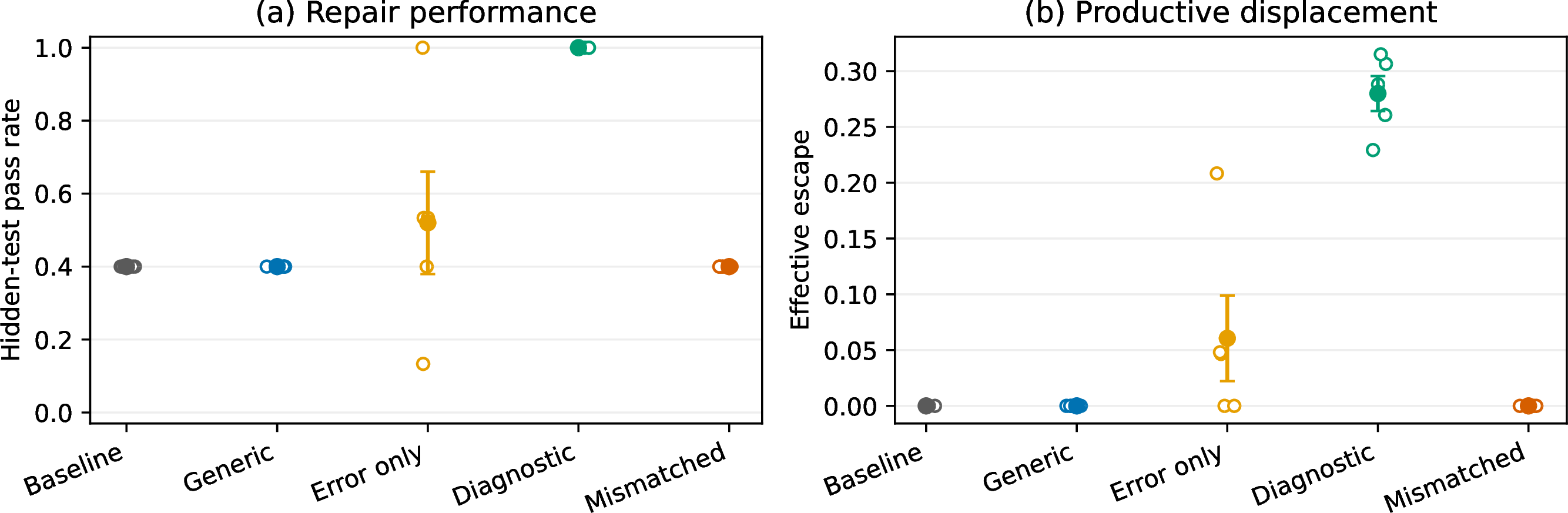
Figure 1: Feedback-induced escape in LLM code repair. Results are computed over five independent Phase 1 trajectories per task; points denote trajectories and filled markers show mean \(\pm\)
SEM. Left: on naturalsize, targeted error feedback improves repair performance, whereas generic and mismatched feedback do not. Right: on pathspec, error-only feedback is unreliable across trajectories, while root-cause diagnostic
feedback achieves successful escape in all five trajectories. Generic feedback can produce substantial code displacement without positive effective escape..
| Task | Condition | Traj. | Pass rate | \(\Delta Q\) | \(E_{\mathrm{eff}}\) |
|---|---|---|---|---|---|
| naturalsize | Baseline | 5 | \(0.143 \pm 0.000\) | \(0.000 \pm 0.000\) | \(0.000 \pm 0.000\) |
| Generic | 5 | \(0.143 \pm 0.000\) | \(0.000 \pm 0.000\) | \(0.000 \pm 0.000\) | |
| Error-only | 5 | \(0.469 \pm 0.045\) | \(0.326 \pm 0.045\) | \(0.052 \pm 0.010\) | |
| Mismatched | 5 | \(0.137 \pm 0.006\) | \(-0.006 \pm 0.006\) | \(0.000 \pm 0.000\) | |
| pathspec | Baseline | 5 | \(0.400 \pm 0.000\) | \(0.000 \pm 0.000\) | \(0.000 \pm 0.000\) |
| Generic | 5 | \(0.400 \pm 0.000\) | \(0.000 \pm 0.000\) | \(0.000 \pm 0.000\) | |
| Error-only | 5 | \(0.520 \pm 0.140\) | \(0.120 \pm 0.140\) | \(0.061 \pm 0.038\) | |
| Diagnostic | 5 | \(1.000 \pm 0.000\) | \(0.600 \pm 0.000\) | \(0.280 \pm 0.016\) | |
| Mismatched | 5 | \(0.400 \pm 0.000\) | \(0.000 \pm 0.000\) | \(0.000 \pm 0.000\) |
6.1.0.3 Results.
Both tasks exhibit stable but incorrect Phase 1 checkpoints. On naturalsize, baseline and generic continuation remain at a pass rate of \(0.143\), while targeted error feedback raises performance to \(0.469 \pm 0.045\). The paired improvement is \(\Delta Q=0.326 \pm 0.045\), with a trajectory-bootstrap \(95\%\) confidence interval of \([0.240,0.394]\). Generic feedback induces substantial code displacement but no quality improvement, and therefore has zero effective escape.
The cross-repository pathspec task reveals a sharper dependence on information content. Baseline, generic, and mismatched feedback all remain at \(0.400\) across every trajectory. Error-only feedback is
unstable, ranging from unsuccessful or regressive revisions to complete repair; its mean gain is only \(0.120 \pm 0.140\), and its bootstrap confidence interval \([-0.107,0.387]\) includes
zero. In contrast, root-cause diagnostic feedback reaches a pass rate of \(1.000\) in all five trajectories, yielding \(\Delta Q=0.600\) and \(E_{\mathrm{eff}}=0.280 \pm 0.016\).
These results refine the escape hypothesis: task relevance alone does not guarantee reliable escape. Feedback must provide information aligned with the task-specific failure boundary. Generic perturbations move the generated code without improving correctness, and shallow error reports may succeed sporadically; sufficiently diagnostic feedback instead produces consistent, quality-aligned state-space escape. These experiments do not by themselves establish a governing-structure shift, which would additionally require the probe-kernel test in Equation 5 .
6.1.0.4 Reproducibility.
All Phase 1 trajectories, Phase 2 samples, hidden-test outcomes, token usage, estimated costs, and task-screening decisions are stored in SQLite. The screening records preserve each candidate task and its inclusion or exclusion reason; no claim of preregistration is made for the present exploratory task selection.
6.2 Experiment 2: Feedback-Driven Escape in Reinforcement Learning↩︎
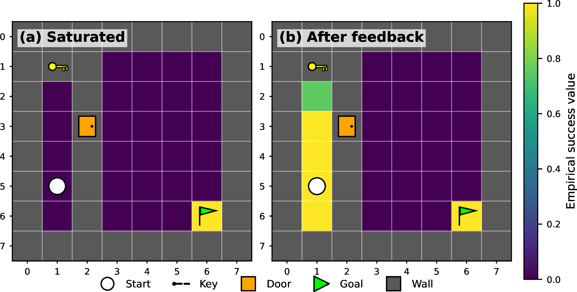
We next examine whether task-relevant feedback can move a saturated policy into a successful behavioral regime, and whether this relocation persists after standard reinforcement learning resumes. We use MiniGrid-DoorKey-8x8-v0, where the
agent must complete the compositional sequence \[\text{pick up key}
\;\rightarrow\;
\text{open door}
\;\rightarrow\;
\text{reach goal}.\] All results are reported over five paired seeds \(\{7,17,42,101,137\}\).
6.2.0.1 Saturated checkpoint.
For each seed, we train PPO using the original sparse reward and evaluate the policy every \(10{,}000\) environment steps. We declare saturation when the success-rate range over five consecutive evaluations is below \(0.05\). All five policies satisfy this criterion at \(50{,}000\) steps while retaining zero task success. Every intervention branch is initialized from its corresponding saturated checkpoint.
6.2.0.2 Feedback and continuation protocols.
Targeted feedback consists of state–action examples generated by a deterministic expert with access to the key, door, and goal locations. The expert demonstrates the task-specific action sequence required for completion. We consider feedback budgets \[m\in\{0,1000,10000,20000\}.\] Behavior cloning (BC) updates the policy on these examples without reward shaping or additional environment interaction.
We compare three protocols. PPO-only continues training directly from the saturated checkpoint for another \(100{,}000\) environment steps. BC-only evaluates the policy immediately after feedback. BC+PPO first applies BC and then resumes PPO for the same \(100{,}000\)-step budget using only the original sparse reward. PPO-only and BC+PPO use the same learning rate, evaluation schedule, continuation budget, and freshly initialized optimizer; they differ only in whether targeted feedback is received before continuation.
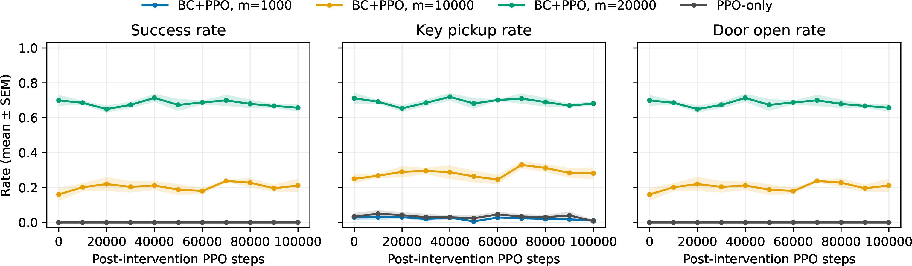
Policies are evaluated every \(10{,}000\) continuation steps over 100 deterministic episodes from a common held-out evaluation stream. We measure task success and the two principal subgoals: \[Q_{\mathrm{succ}} = \Pr(\text{reach goal}),\qquad Q_{\mathrm{key}} = \Pr(\text{pick up key}),\qquad Q_{\mathrm{door}} = \Pr(\text{open door}).\] Values are reported as mean \(\pm\) SEM over the five paired seeds. To characterize post-feedback relaxation, we additionally report the mean success over the final three evaluations (Tail-3) and the step-normalized area under the continuation curve (AUC).
| Protocol | Immediate | Final | Tail-3 | AUC |
|---|---|---|---|---|
| PPO-only, \(m=0\) | \(0.000\pm0.000\) | \(0.000\pm0.000\) | \(0.000\pm0.000\) | \(0.000\pm0.000\) |
| BC+PPO, \(m=1000\) | \(0.000\pm0.000\) | \(0.000\pm0.000\) | \(0.000\pm0.000\) | \(0.000\pm0.000\) |
| BC+PPO, \(m=10000\) | \(0.160\pm0.036\) | \(0.212\pm0.038\) | \(0.212\pm0.024\) | \(0.205\pm0.016\) |
| BC+PPO, \(m=20000\) | \(0.700\pm0.031\) | \(0.658\pm0.022\) | \(0.669\pm0.011\) | \(0.681\pm0.016\) |
6.2.0.3 Results.
Additional optimization alone does not escape the saturated regime. PPO-only continuation remains at zero success for every seed despite receiving another \(100{,}000\) environment steps. Weak feedback is likewise insufficient: with \(m=1000\), both immediate and post-continuation success remain zero. Thus, reopening the optimizer cannot compensate for feedback that fails to establish a useful behavioral hypothesis.
At \(m=10000\), BC immediately raises success to \(0.160\pm0.036\). After resumed PPO, final success reaches \(0.212\pm0.038\), with Tail-3 \(0.212\pm0.024\) and AUC \(0.205\pm0.016\). Final key-pickup and door-open rates are \(0.282\pm0.034\) and \(0.212\pm0.038\), respectively. Intermediate feedback therefore establishes a nonzero-success region that remains accessible during subsequent sparse-reward learning, although the seed-level change from immediate to final performance is variable.
At \(m=20000\), immediate success reaches \(0.700\pm0.031\). The policy remains in a high-success regime throughout continuation, with final success \(0.658\pm0.022\), Tail-3 \(0.669\pm0.011\), and AUC \(0.681\pm0.016\). Final key pickup and door opening reach \(0.682\pm0.012\) and \(0.658\pm0.022\), respectively. Door opening and task success are nearly identical, indicating that once the key–door sequence is completed, reaching the goal is rarely the remaining bottleneck.
The strongest-feedback branch does not improve monotonically under resumed PPO: its final success is slightly below its immediate BC performance. We therefore interpret the result as persistent basin relocation, rather than as evidence that post-feedback optimization must monotonically improve the policy. The matched-budget controls separate reopening the learning loop from the informational effect of feedback: additional PPO alone is insufficient, whereas sufficiently strong task-relevant feedback moves the policy into a successful behavioral region that subsequent sparse-reward learning can preserve.
6.2.0.4 Reproducibility.
The experiment contains 40 seed–protocol units. Per-seed checkpoints, evaluation trajectories, subgoal rates, relaxation summaries, and run metadata are stored in SQLite and exported as machine-readable tables. All continuation branches use the same environment, sparse reward, evaluation stream, and training budget.
6.3 Information-Driven Escape in Bayesian Optimization↩︎
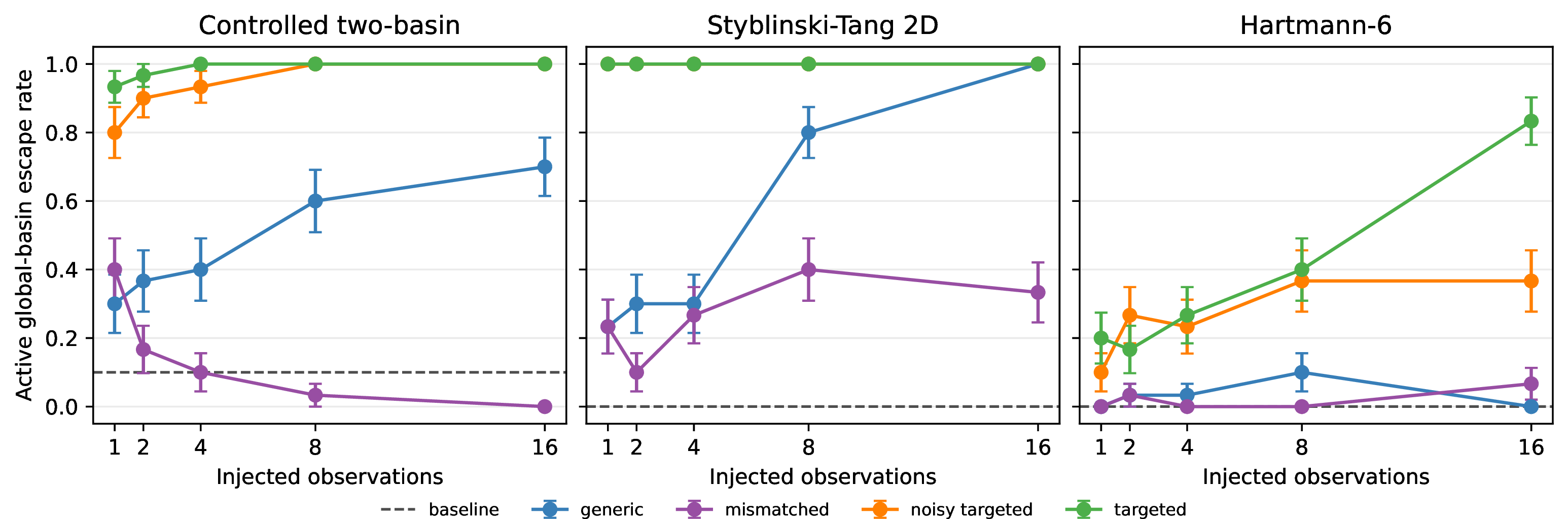
We use Bayesian optimization (BO) to separate the informational effect of feedback from the effect of reopening the search space. For each task and seed, Phase 1 restricts expected-improvement BO to a local trust region centered on a suboptimal minimum, producing a controlled locally saturated checkpoint. In Phase 2, the constraint is removed for all branches, including the no-feedback baseline, and each branch receives 12 real BO queries over the full domain.
We evaluate a controlled two-basin objective, Styblinski–Tang 2D, and Hartmann–6 using 30 paired evaluation seeds, disjoint from the five calibration seeds. We compare Baseline, Generic, Targeted, Noisy-Targeted, and Mismatched feedback, with information amount \(m\in\{1,2,4,8,16\}\). Injected observations update the GP posterior but do not count as objective queries or realized improvements. They are excluded from query de-duplication, allowing BO to actively query and verify a feedback-indicated hypothesis.
An active escape occurs only when a real Phase 2 query enters the pre-specified global basin: \[A_{s,c,m} = \mathbb{I}\!\left[ \exists t: x^{\mathrm{query}}_{s,c,m,t} \in \mathcal{B}_{\mathrm{global}} \right].\] Let \(R_{s,c,m}\) be the best post-intervention query regret. We define \[\Delta Q_{s,c,m} = R_{s,\mathrm{base},0}-R_{s,c,m}, \qquad E^{\mathrm{eff}}_{s,c,m} = A_{s,c,m}\max(\Delta Q_{s,c,m},0).\] Thus, posterior displacement without active verification and positive quality improvement does not count as effective escape.
| Task | Baseline | T\(_1\) | T\(_{16}\) | G\(_1\) | G\(_{16}\) | M\(_{16}\) |
|---|---|---|---|---|---|---|
| Controlled two-basin | .100 | .933 | 1.000 | .300 | .700 | .000 |
| Styblinski–Tang 2D | .000 | 1.000 | 1.000 | .233 | 1.000 | .333 |
| Hartmann–6 | .000 | .200 | .833 | .000 | .000 | .067 |
Reopening the domain alone is generally insufficient: baseline escape is zero on Styblinski–Tang and Hartmann–6 and only 0.10 on the controlled task. A single targeted observation raises escape to 0.933 on the controlled task and 1.0 on Styblinski–Tang. Hartmann–6 exhibits a higher information requirement: targeted escape rises from 0.20 at \(m=1\) to 0.833 at \(m=16\), while generic feedback remains ineffective.
Large amounts of generic information can nevertheless induce escape on simpler landscapes, reaching 0.70 on the controlled task and 1.0 on Styblinski–Tang at \(m=16\). Thus, targeted information is not strictly necessary. Instead, alignment shifts the information–escape frontier: task-aligned feedback requires less information to induce active verification and quality improvement, while the required information level remains task dependent.
7 Discussion↩︎
7.0.0.1 Scope and positioning.
The framework gives sufficient conditions and operational diagnostics for saturation and escape, not a full classification of all possible closed-loop dynamics. It does not characterize oscillation, divergence, or adversarial feedback, and Section 5 analyzes a single external perturbation rather than a sequence of interacting perturbations. The information-theoretic bound also assumes a bounded representation space only when converting expected metric displacement into an escape-probability bound. The direct event-level KL threshold does not require bounded \(\mathcal{X}\). Structural identifiability is relative to the declared probe distribution \(\mu\): no black-box experiment can distinguish parameter values that induce the same transition law on all probed states.
7.0.0.2 Extensions.
The framework is instantiated in three distinct settings: LLM code repair, reinforcement learning, and Bayesian optimization. Future extensions include active learning, curriculum learning, and multi-agent feedback loops.
7.0.0.3 Empirical status of the structural and information quantities.
The current experiments measure escape outcomes and feedback budgets, but do not yet estimate \(\delta_{\mu,\nu}\) or the baseline-relative KL in Equation ?? . Accordingly, they support the saturation–escape phenomenology but should not be read as direct validation of a governing-structure change or of the numerical information-divergence threshold. A direct test would pre-register probe states, resample transitions before and after intervention to estimate Equation 5 , and estimate escape probabilities or density ratios relative to matched no-intervention continuations.
7.0.0.4 Conclusion.
We introduced an operational framework for closed-loop knowledge dynamics based on representations, parameterized transition kernels, and a governing parameter identifiable up to observational equivalence. Classical Lyapunov drift conditions characterize fixed-parameter saturation, while pre-registered kernel discrepancies distinguish structural change from transient state movement. Escape is evaluated separately as a quality-aligned probability change relative to a matched no-intervention law, for which baseline-relative KL—rather than mutual information alone—provides the relevant information cost. The resulting contribution is a common measurement and intervention language for heterogeneous closed-loop systems, supported by cross-domain experiments and designed for direct empirical refinement.
8 Deferred Proofs↩︎
8.0.0.1 Proof of Proposition 1.
Taking expectation in the assumed drift inequality gives \(\mathbb{E}[d(x_{t+1},x^\star)] \le \rho \mathbb{E}[d(x_t,x^\star)] + \sigma\). Unrolling the recursion yields \[\mathbb{E}[d(x_t,x^\star)] \le \rho^t d(x_0,x^\star) + \sum_{s=0}^{t-1}\rho^s\sigma = \rho^t d(x_0,x^\star) + \frac{\sigma(1-\rho^t)}{1-\rho}.\] For the step size, by the triangle inequality, \(d(x_t,x_{t+1}) \le d(x_t,x^\star)+d(x_{t+1},x^\star)\). Taking expectations and applying the previous bound to both terms gives \[\Delta_t \le \mathbb{E}[d(x_t,x^\star)] + \mathbb{E}[d(x_{t+1},x^\star)] \le (1+\rho)\rho^t d(x_0,x^\star) + \frac{2\sigma}{1-\rho}.\]
8.0.0.2 Proof of Proposition 3.
Since \(x_{t_0}\in B(x^\ast_{\theta},c)\), the triangle inequality gives \(d(x_{t_0}, x^\ast_{\theta'}) \le c + \Delta\). One step of the perturbed contraction then gives \(\mathbb{E}[d(x_{t_0+1}, x^\ast_{\theta'})] \le \rho'(c+\Delta) + \sigma_{\mathrm{ext}}\). Applying the triangle inequality once more, \[\mathbb{E}[d(x_{t_0+1}, x^\ast_{\theta})] \ge \Delta - \mathbb{E}[d(x_{t_0+1}, x^\ast_{\theta'})] \ge \Delta - \rho'(c+\Delta) - \sigma_{\mathrm{ext}}.\] The right-hand side exceeds \(c\) exactly when \(\Delta > \Delta^\ast\).
Remark 6 (Local linearization). When \(\mathcal{X}\) is a vector space or smooth manifold and \(\mathcal{T}_{\omega}\) is differentiable near a fixed point \(x^\star\), local stability can be checked through the Jacobian \[J_\star = D_x\mathcal{T}_{\omega}(x^\star).\] Writing \(\delta x_{t+1}\approx J_\star\delta x_t\), the quadratic Lyapunov function \(V(x)=\|x-x^\star\|^2\) gives local contraction whenever the spectral radius satisfies \(\rho(J_\star)<1\). The eigenvectors of \(J_\star\) identify directions of fast and slow decay. This provides a differentiable analogue of the metric contraction condition used below for text-space self-refinement.
8.1 Additional Validation A: Cross-System Saturation Signatures↩︎
![Figure 5: Saturation signatures across three closed-loop systems. (a) LLM self-refinement: transition magnitude decays toward a residual floor. (b) RL value iteration: Bellman update magnitude decays geometrically. (c) Bayesian optimization: exploration pressure W_t=\beta_t\mathbb{E}[\sigma_t] decays as posterior uncertainty is resolved. Together, these examples show saturation across text refinement, value-function iteration, and belief-guided search.](/article/2607.14185/fig_saturation_across_systems.png "fig:")
We first test whether the saturation signature predicted by Theorem 1 appears across qualitatively different closed-loop systems. We consider three cases: recursive LLM self-refinement, tabular RL value iteration, and belief-guided Bayesian optimization. These systems differ in state space and feedback mechanism, but each repeatedly updates an internal knowledge representation under fixed governing dynamics. For LLM self-refinement, the state \(x_t\) is a draft and the transition magnitude is measured as \(\Delta_t=d(x_t,x_{t+1})\). For RL, the state is the value function and we track the Bellman update magnitude \(\|V_{t+1}-V_t\|_\infty\). For Bayesian optimization, the state is a Gaussian process posterior and we track the exploration pressure \(W_t=\beta_t\mathbb{E}[\sigma_t]\). Figure 5 shows that all three systems exhibit a saturation pattern. LLM self-refinement follows an exponential-plus-floor curve, RL value iteration shows rapid geometric decay, and Bayesian optimization exhibits power-law attenuation of exploration pressure. These results support the claim that saturation is a general closed-loop phenomenon rather than an artifact of a single model or task.
8.2 Additional Validation B: Escape in Recursive Abstract Refinement↩︎
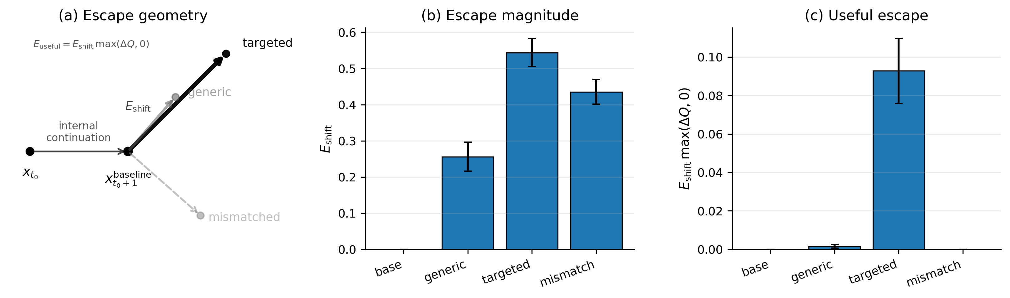
We next test whether external feedback can move a saturated self-refinement trajectory beyond its internal continuation baseline. After recursive self-refinement reaches a low-change regime at round \(t_0\), we compare four conditions: baseline continuation, generic feedback, targeted feedback, and mismatched feedback. We define escape magnitude as \[E_{\mathrm{shift}} = d\!\left( x_{t_0+1}^{\mathrm{condition}}, x_{t_0+1}^{\mathrm{baseline}} \right),\] where \(x_{t_0+1}^{\mathrm{baseline}}\) is the output produced by continuing internal self-refinement without external feedback. To distinguish mere displacement from useful escape, we also compute \[E_{\mathrm{useful}} = E_{\mathrm{shift}}\max(\Delta Q,0),\] where \(\Delta Q\) is the quality gain relative to the baseline continuation.
Figure 6 shows that targeted feedback produces the largest escape magnitude, approximately \(0.54\), compared with approximately \(0.26\) for generic feedback and \(0.43\) for mismatched feedback. The mismatched condition demonstrates that irrelevant feedback can still induce a large state displacement. However, useful escape is concentrated almost entirely in the targeted-feedback condition, with mean useful escape approximately \(0.09\), whereas generic and mismatched feedback produce near-zero useful escape. These results support the prediction that successful escape requires external information that is both strong enough to perturb the saturated trajectory and relevant enough to improve it.
8.3 Additional Validation C: Post-Perturbation Relaxation↩︎
We finally test whether successful external perturbation induces a renewed relaxation phase after saturation. Under fixed governing dynamics, recursive self-refinement should approach a low-change regime. If targeted external feedback shifts the effective transition regime, then the transition magnitude should exhibit a spike at the perturbation round followed by a second decay phase.
For each item, we run recursive self-refinement until round \(t_0\), where the transition magnitude has reached a small residual floor. We then compare two continuations: a baseline trajectory that continues internal self-refinement without external feedback, and a targeted-perturbation trajectory that receives external feedback at round \(t_0\) before continuing internal refinement. We track \[\Delta_t=d(x_t,x_{t-1})\] over the full trajectory. To quantify relaxation before and after the perturbation, we fit exponential-plus-floor curves: \[\Delta_t^{\mathrm{pre}} \approx A_1 e^{-k_1t}+c_1, \qquad \Delta_t^{\mathrm{post}} \approx A_2 e^{-k_2(t-t_0-1)}+c_2.\]
Table 4 shows the predicted double-saturation pattern. The pre-perturbation trajectory decays toward a small floor, indicating saturation under internal feedback. The targeted perturbation produces a spike in transition magnitude above the saturated floor, while the baseline continuation remains near the floor. After the perturbation, the transition magnitude decays again, producing a second relaxation phase. This provides an observable candidate signature for renewed relaxation: the external input moves the system away from its internal continuation, and the subsequent internal loop relaxes toward a new locally stable regime. Under Equation 5 , however, a spike and second decay alone do not establish a governing-structure shift; that claim requires a reproducible post-intervention kernel discrepancy on pre-specified probes.
| Condition | Spike magnitude \(\uparrow\) | Spike rate \(\uparrow\) | Post-fit \(R^2\) | Final \(\Delta_T\) \(\downarrow\) |
|---|---|---|---|---|
| Baseline continuation | 0.004 \(\pm\) 0.002 | 0.07 | – | 0.006 \(\pm\) 0.001 |
| Generic feedback | 0.026 \(\pm\) 0.006 | 0.38 | 0.841 | 0.010 \(\pm\) 0.003 |
| Targeted perturbation | 0.071 \(\pm\) 0.009 | 0.93 | 0.962 | 0.008 \(\pm\) 0.002 |
| Mismatched feedback | 0.049 \(\pm\) 0.008 | 0.71 | 0.624 | 0.021 \(\pm\) 0.005 |
Together with Experiment 2, this result distinguishes useful escape from mere perturbation. Experiment 2 shows that targeted feedback produces the largest useful escape magnitude, while Experiment 3 shows that such perturbations can initiate a renewed relaxation phase rather than simply increasing noise.